Computing all Space Curve Solutions of Polynomial Systems by Polyhedral Methods

Abstract

A polyhedral method to solve a system of polynomial equations exploits its sparse structure via the Newton polytopes of the polynomials. We propose a hybrid symbolic-numeric method to compute a Puiseux series expansion for every space curve that is a solution of a polynomial system. The focus of this paper concerns the difficult case when the leading powers of the Puiseux series of the space curve are contained in the relative interior of a higher dimensional cone of the tropical prevariety. We show that this difficult case does not occur for polynomials with generic coefficients. To resolve this case, we propose to apply polyhedral end games to recover tropisms hidden in the tropical prevariety.

Key words and phrases. Newton polytope, polyhedral end game, polyhedral method, polynomial system, Puiseux series, space curve, tropical basis, tropical prevariety, tropism.

1 Introduction

In this paper we consider the application of polyhedral methods to compute series for all space curves defined by a polynomial system. Polyhedral methods compute with the Newton polytopes of the system. The Newton polytope of a polynomial is defined as the convex hull of the exponents of the monomials that appear with a nonzero coefficient.

If we start the development of the series where the space curve meets the first coordinate plane, then we compute Puiseux series. Collecting for each coordinate the leading exponents of a Puiseux series gives what is called a tropism. If we view a tropism as a normal vector to a hyperplane, then we see that there are hyperplanes with this normal vector that touch every Newton polytope of the system at an edge or at a higher dimensional face. A vector normal to such a hyperplane is called a pretropism. While every tropism is a pretropism, not every pretropism is a tropism.

In this paper we investigate the application of a polyhedral method to compute all space curve solutions of a polynomial system. The method starts from the collection of all pretropisms, which are regarded as candidate tropisms. For the method to work, we focus on the following questions.

Problem Statement. Given that only the space curves are of interest, can we ignore the higher dimensional cones of pretropisms? In particular, if some tropisms lie in the interior of higher dimensional cones of pretropisms, is it then still possible to compute Puiseux series solutions for all space curves?

Related Work. In symbolic computation, new elimination algorithms for sparse systems with positive dimensional solution sets are described in [8]. Tropical resultants are computed in [13]. Related polyhedral methods for sparse systems can be found in [10, 15]. Conditions on how far a Puiseux series should be expanded to decide whether a point is isolated are given in [6]. The authors of [12] propose numerical methods for tropical curves. Polyhedral methods to compute tropical varieties are outlined in [4] and implemented in Gfan [14]. The background on tropical algebraic geometry is in [16].

Algorithms to compute the tropical prevariety are presented in [21]. For preprocessing purposes, the software of [21] is useful. However, the focus on this paper concerns the tropical variety for which Gfan [14] provides a tropical basis. Therefore, our computational experiments with computer algebra methods are performed with Gfan and not with the software of [21].

Organization and Contributions. In the next section we illustrate the advantages of looking for Puiseux series as solutions of polynomial systems. Then we motivate our problem with some illustrative examples. Relating the tropical prevariety to a recursive formula to compute the mixed volume characterizes the generic case, in which the tropical prevariety suffices to compute all space curve solutions. With polyhedral end games we can recover the tropisms contained in higher dimensional cones of the tropical prevariety. Finally we give some experimental results and timings.

2 Puiseux Series

When we work with Puiseux series we apply a hybrid method, combining exact and approximate calculations. Figure 1 shows the plot, in black, of Viviani’s curve, defined as the intersection of the sphere $f=x_{1}^{2}+x_{2}^{2}+x_{3}^{2}-4=0$ and the cylinder $g=(x_{1}-1)^{2}+x_{2}^{2}-1=0$.

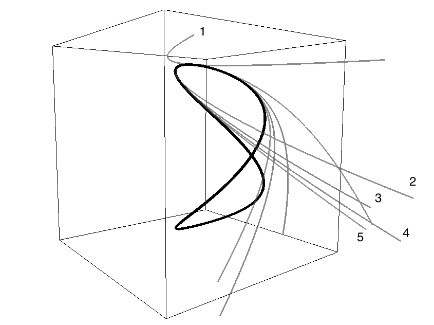
Figure 1: Viviani’s curve with improving Puiseux series approximations, labelled with the number of terms used to plot each one.

There is one pretropism $\mathbf{v}=(2,1,0)$, which defines the initial forms of $f$ and $g$ respectively as $x_{3}^{2}-4$ and $x_{2}^{2}-2x_{1}$. For traditional Puiseux series, one would choose to set $x_{1}=1$, obtaining the four solutions $(1,\pm\sqrt{2},\pm 2)$ and leading terms $(t^{2},\pm\sqrt{2}t,\pm 2)$. If we instead use $x_{1}=2$, we obtain rational coefficients and the following partial expansion:

$$\left[\begin{array}[]{c}x_{1}\\ x_{2}\\ x_{3}\end{array}\right]=\left[\begin{array}[]{c}2t^{2}\\ 2t-t^{3}-\frac{1}{4}t^{5}-\frac{1}{8}t^{7}-\frac{5}{64}t^{9}\\ 2-t^{2}-\frac{1}{4}t^{4}-\frac{1}{8}t^{6}-\frac{5}{64}t^{9}\end{array}\right].$$ (1)

The plot of several Puiseux approximations to Viviani’s curve is shown in gray in Figure 1.

If we shift the Viviani example so that its self-intersection is at the origin, we obtain the following:

$$\mathbf{f}(\mathbf{x})=\left\{\begin{array}[]{r}x_{1}^{2}+x_{2}^{2}+x_{3}^{2}+4x_{1}=0\\ x_{1}^{2}+x_{2}^{2}+2x_{1}=0\end{array}\right.$$ (2)

An examination of the first few terms of the Puiseux series expansion for this system, combined with the On-Line Encyclopedia of Integer Sequences [17] and some straightforward algebraic manipulation, allows us to hypothesize the following exact parameterization of the variety:

$$\left[\begin{array}[]{c}x_{1}\\ x_{2}\\ x_{3}\end{array}\right]=\left[\begin{array}[]{c}-2t^{2}\\ 2\frac{t^{3}}{1+\sqrt{1-t^{2}}}\;-\;2t\\ -2t\end{array}\right].$$ (3)

We can confirm that this is indeed right via substitution. While this method is of course not possible in general, it does provide an example of the potential usefulness of Puiseux series computations for some examples.

3 Assumptions and Setup

Our object of study is space curves, by which we mean 1-dimensional varieties in $\mathbb{C}^{n}$. Because Puiseux series computations take one variable to be a free variable, we require that the curves not lie inside $V(\langle x_{i}\rangle)$ for some $i$; without loss of generality we choose to use the first variable. Some results require that the curve be in Noether position with respect to $x_{1}$, meaning that the degree of the variety is preserved under intersection with $x_{1}=\lambda$ for a generic $\lambda\in\mathbb{C}$. It is of course possible to apply a random coordinate transformation to obtain Noether position, but we then lose the sparsity of the system’s exponent support structure, which is what makes polyhedral methods effective.

4 Some Motivating Examples

In this section we illustrate the problem our paper addresses with some simple examples, first in 3-space, and then with a family of space curves in any dimensional space.

4.1 In 3-Space

Our first running example is the system

$$\mathbf{f}(\mathbf{x})=\left\{\begin{array}[]{r}x_{1}x_{3}-x_{2}x_{3}-x_{3}^{2}+x_{1}=0\\ x_{3}^{3}-x_{1}x_{2}-x_{2}x_{3}-x_{3}^{2}-x_{1}=0\end{array}\right.$$ (4)

which has an irreducible quartic and the second coordinate axis $(0,x_{2},0)$ as its solutions. Because the line lies in the first coordinate plane $x_{1}=0$, the system is not in Noether position with respect to the first variable. Therefore, our methods will ignore this part of the solution set. The algorithms of [7] can be applied to compute components inside coordinate planes. Computing a primary decomposition yields the following alternative, which lacks the portion in the first coordinate plane:

$$\bf\tilde{f}(\mathbf{x})=\left\{\begin{array}[]{r}x_{1}x_{3}-x_{2}x_{3}-x_{3}^{2}+x_{1}\\ x_{1}x_{2}-x_{2}^{2}-x_{2}x_{3}+x_{3}^{2}+x_{1}-2x_{2}-2x_{3}\\ x_{3}^{3}-x_{2}^{2}-2x_{2}x_{3}-2x_{2}-2x_{3}\end{array}\right.$$ (5)

The tropical prevariety contains the rays $(2,1,1)$, $(1,0,0)$, and $(1,0,1)$; because our Puiseux series start their development at $x_{1}=0$, rays that have a zero or negative value for their first coordinate have been discarded. The tropical variety however contains the ray $(3,1,1)$ instead of $(2,1,1)$, leading to the Puiseux expansion

$$\left[\begin{array}[]{c}x_{1}\\ x_{2}\\ x_{3}\end{array}\right]=\left[\begin{array}[]{c}108t^{3}\\ t-3t^{2}-15t^{3}+27t^{4}+36t^{5}\\ -t-3t^{3}-18t^{4}+18t^{5}+162t^{6}\end{array}\right].$$ (6)

This ray is a positive combination of $(2,1,1)$ and $(1,0,0)$. In other words, it is possible for the 1-dimensional cones of the tropical prevariety to fail to be in the tropical variety, and for rays in the tropical variety to “hide” in the higher-dimensional cones of the prevariety.

4.2 In Any Dimensional Space

This problem can also occur in arbitrary dimensions, as seen in the class of examples

$$\mathbf{f}(\mathbf{x})=\left\{\begin{array}[]{rcl}x_{1}^{2}-x_{1}+x_{2}+x_{3}+\cdots+x_{n}&=&0\\ x_{2}^{2}+x_{1}+x_{2}+x_{3}+\cdots+x_{n}&=&0\\ x_{3}^{2}+x_{1}+x_{2}+x_{3}+\cdots+x_{n}&=&0\\ &\vdots&\\ x_{n-1}^{2}+x_{1}+x_{2}+x_{3}+\cdots+x_{n}&=&0.\end{array}\right.$$ (7)

The ray $(1,1,1,\ldots,1)$ is a 1-dimensional cone of its prevariety since it is normal to a facet of each polytope, namely the linear portion of each polynomial. It is not, however, in the tropical variety, since the initial form system (as it will be defined in Section 5) contains the monomial $x_{1}$.

5 The Generic Case

This hiding of tropisms in the higher dimensional cones of the prevariety is problematic, as finding the tropical variety may require more expensive symbolic computations. For a comparison between various approaches see Section 9. Fortunately, this problem does not occur in general, as the next result will show. But first, a few definitions.

Definition 5.1.

We write a polynomial $f$ with support set $A$ as

$$f(\mathbf{x})=\sum_{\mathbf{a}\in A}c_{\mathbf{a}}\mathbf{x}^{\mathbf{a}},\quad c_{\mathbf{a}}\in{\mathbb{C}}^{*},\mathbf{x}^{\mathbf{a}}=x_{1}^{a_{1}}x_{2}^{a_{2}}\cdots x_{n}^{a_{n}}.$$ (8)

The initial form of $f$ with respect to $\mathbf{v}$ is then

$${\rm in}_{\mathbf{v}}f(\mathbf{x})=\sum_{\mathbf{a}\in{\rm in}_{\mathbf{v}}A}c_{\mathbf{a}}\mathbf{x}^{\mathbf{a}},$$ (9)

where $\displaystyle{\rm in}_{\mathbf{v}}A=\{\ \mathbf{a}\in A\ |\ \langle\mathbf{a},\mathbf{v}\rangle=\min_{\mathbf{b}\in A}\langle\mathbf{b},\mathbf{v}\rangle\ \}$.

The initial form of a tuple of polynomials is the tuple of the initial forms of the polynomials in the tuple.

Definition 5.2.

For $f\in\mathbb{C}[{\bf x}]$, $I$ an ideal in $\mathbb{C}[{\bf x}]$ and ${\bf v}\in\mathbb{R}^{n}$, we define the initial ideal $\text{in}_{\bf v}(I)$ as the ideal generated by $\{\text{in}_{\bf v}(f):f\in I\}$.

Definition 5.3.

For $I=\langle f_{1},\ldots,f_{m}\rangle\subset\mathbb{C}[{\bf x}]$ an ideal, the tropical prevariety is the set of ${\bf v}\in\mathbb{R}^{n}$ for which $\text{in}_{\bf v}(f_{i})$ is not a monomial for any $i$. The tropical variety is the set of ${\bf v}\in\mathbb{R}^{n}$ for which $\text{in}_{\bf v}(f)$ is not a monomial for any $f\in I$.

Proposition 5.4.

For $n$ equations in $n+1$ unknowns with generic coefficients, the set of ray generators of the tropical prevariety contains the tropical variety.

It is important to note that our notion of generic here refers to the coefficients, and not to generic tropical varieties as seen in [18] which are tropical varieties of ideals under a generic linear transformation of coordinates.

The tropical prevariety always contains the tropical variety. We simply want to show that all of the rays of the tropical variety show up in the prevariety as ray generators, and not as members of the higher-dimensional cones. Let $I=\langle p_{1},\ldots,p_{n}\rangle\subseteq\mathbb{C}[x_{0},\ldots,x_{n}]$, and let $\mathbf{w}$ be a ray in the tropical prevariety but not one of its ray generators. We want to show that $\mathbf{w}$ is not in the tropical variety, or equivalently that $\text{in}_{\mathbf{w}}(I)$ contains a monomial. We will do so by showing that $I_{\mathbf{w}}:=\langle\text{in}_{\mathbf{w}}(p_{1}),\ldots,\text{in}_{\mathbf{w}}(p_{n})\rangle$ contains a monomial, which suffices since this ideal is contained in $\text{in}_{\mathbf{w}}(I)$.

Suppose $I_{\mathbf{w}}$ contains no monomial. Then $(x_{0}x_{1}\cdots x_{n})^{k}\notin I_{\mathbf{w}}$ for any $k$. By Hilbert’s Nullstellensatz $V:=\mathbb{V}(I_{\mathbf{w}})\nsubseteq\mathbb{V}(x_{0}x_{1}\cdots x_{n})$, i.e. $V$ is not contained in the union of the coordinate hyperplanes. Then there exists $a=(a_{0},\ldots,a_{n})\in V$ such that all coordinates of $a$ are all nonzero. Since $\mathbf{w}$ lies in the interior a cone of dimension at least 2, the generators of $I_{\mathbf{w}}$ are homogeneous with respect to at least two linearly independent rays u and v. Thus $(\lambda^{\mathbf{u}_{0}}\mu^{\mathbf{v}_{0}}a_{0},\ldots,\lambda^{\mathbf{u}_{n}}\mu^{\mathbf{v}_{n}}a_{n})\in V$ for all $\lambda,\mu\in\mathbb{C}\setminus\{0\}$ where the $\mathbf{u}_{i},\mathbf{v}_{i}$ are the components of $\bf u$ and $\bf v$, and $V$ contains a toric surface. If we intersect with a random hyperplane, by Bernstein’s theorem B [3] the result is a finite set of points, with the possibility of additional components that must be contained in the coordinate planes. Hence $V$ can contain no surface outside of the coordinate planes, and we have a contradiction.

∎

6 Polyhedral Methods

We will show that the tropical prevariety provides an upper bound for the degree of the solution curve. The inner product of a point $\mathbf{a}$ with a vector $\mathbf{v}$ is denoted as $\langle\mathbf{a},\mathbf{v}\rangle=a_{1}v_{1}+a_{2}v_{2}+\cdots+a_{n}v_{n}$.

Lemma 6.1.

Consider an $(n-1)$-tuple of Newton polytopes ${\cal P}=(P_{1},P_{2},\ldots,P_{n-1})$ in $n$-space. Let $E$ be the edge spanned by $(1,0,\ldots,0)$ and $(0,0,\ldots,0)$. The mixed volume of $({\cal P},E)$ equals

$$V_{n}({\cal P},E)=\sum_{\mathbf{v}}v_{1}V_{n-1}({\rm in}_{\mathbf{v}}{\cal P}),$$ (10)

where $\mathbf{v}$ ranges over all rays in the tropical prevariety of $\cal P$ with $v_{1}>0$, normalized so that ${\rm gcd}(\mathbf{v})={\rm gcd}(v_{1},v_{2},\ldots,v_{n})=1$, and ${\rm in}_{\mathbf{v}}{\cal P}=({\rm in}_{\mathbf{v}}P_{1},{\rm in}_{\mathbf{v}}P_{2},\ldots$, ${\rm in}_{\mathbf{v}}P_{n-1})$, where ${\rm in}_{\mathbf{v}}P_{k}$ is the face with support vector $\mathbf{v}$, formally expressed as

$${\rm in}_{\mathbf{v}}P_{k}=\{\ \mathbf{a}\in P_{k}\ |\ \langle\mathbf{a},\mathbf{v}\rangle=\max_{\mathbf{a}\in P_{k}}\langle\mathbf{a},\mathbf{v}\rangle\ \}.$$ (11)

We apply the following recursive formula [20] for the mixed volume

$$V_{n}({\cal P},E)=\sum_{\begin{array}[]{c}\mathbf{v}\in{\mathbb{Z}}^{n}\\ \gcd(\mathbf{v})=1\end{array}}\ p_{E}(\mathbf{v})\ V_{n-1}({\rm in}_{\mathbf{v}}{\cal P}),$$ (12)

where $p_{E}$ is the support function of the edge $E$:

$$p_{E}(\mathbf{v})=\max_{\mathbf{e}\in E}\langle\mathbf{e},\mathbf{v}\rangle$$ (13)

and ${\rm in}_{\mathbf{v}}{\cal P}=({\rm in}_{\mathbf{v}}P_{1},{\rm in}_{\mathbf{v}}P_{2},\ldots,{\rm in}_{\mathbf{v}}P_{n-1})$, where

$${\rm in}_{\mathbf{v}}P_{k}=\{\ \mathbf{a}\in P_{k}\ |\ \langle\mathbf{a},\mathbf{v}\rangle=p_{k}(\mathbf{v})\ \},$$ (14)

with $p_{k}$ the support function of the polytope $P_{k}$.

Because the edge $E$ contains $(0,0,\ldots,0)$: $p_{E}(\mathbf{v})\geq 0$ and $p_{E}(\mathbf{v})=0$ when $v_{1}\leq 0$. Only those rays for which $v_{1}>0$ contribute to $V_{n}({\cal P},E)$. We have then $p_{E}(\mathbf{v})=v_{1}$.

The mixed volume of a tuple of polytopes equals zero if one of the polytopes consists of only one vertex. The rays in the tropical prevariety contain all vectors for which ${\rm in}_{\mathbf{v}}(P_{k})$ is an edge or a higher dimensional face. These are the rays $\mathbf{v}$ for which $V_{n-1}({\rm in}_{\mathbf{v}}{\cal P})>0$.

∎

The application of Lemma 6.1 leads to a bound on the number of generic points on the space curve. Denote ${\mathbb{C}}^{*}={\mathbb{C}}\setminus\{0\}$.

Lemma 6.2.

Consider the system $\mathbf{f}(\mathbf{x})=\mathbf{0}$, $\mathbf{f}=(f_{1}$, $f_{2}$, $\ldots$, $f_{n-1})$ with ${\cal P}=(P_{1},P_{2},\ldots,P_{n-1})$ where $P_{k}$ is the Newton polytopes of $f_{k}$. If the system is in Noether position with respect to $x_{1}$, then the degree of the space curve defined by $\mathbf{f}(\mathbf{x})=\mathbf{0}$ is bounded by $V_{n}({\cal P},E)$.

This result is a version of Lemma 2.3 from [15].

The proof of the lemma follows from the application of Bernshtein’s theorem [3] to the system

$$\left\{\begin{array}[]{l}\mathbf{f}(\mathbf{x})=\mathbf{0}\\ x_{1}=\gamma,\quad\gamma\in{\mathbb{C}}^{*}.\end{array}\right.$$ (15)

By the assumption of Noether position, there will be as many solutions to this system as the degree of the space curve defined by $\mathbf{f}(\mathbf{x})=\mathbf{0}$. The theorem of Bernshtein states that the mixed volume bounds the number of solutions in $({\mathbb{C}}^{*})^{n}$.

∎

Formula (12) appears in the constructive proof of Bernshtein’s theorem [3] and was implemented in the polyhedral homotopies of [25]. For systems with coefficients that are sufficiently generic, the mixed volumes provide an exact root count.

Theorem 6.3.

Let $\mathbf{f}(\mathbf{x})=\mathbf{0}$ be a polynomial system of $n-1$ equations in $n$ unknowns, with sufficiently generic coefficients. Assume the space curve defined by $f(\mathbf{x})=\mathbf{0}$ is in Noether position with respect to the first variable. Then all rays $\mathbf{v}$ with $v_{1}>0$ in the tropical prevariety of $\mathbf{f}$ lead to Puiseux series expansions for the space curve defined by $\mathbf{f}(\mathbf{x})=\mathbf{0}$. Moreover, the degree of the space curve is the sum of the degrees of the Puiseux series.

We illustrate the application of polyhedral methods to the motivating examples.

Example 6.4.

As a verification on the first motivating example (4), we consider the rays $(2,1,1)$, $(1,0,0)$, and $(1,0,1)$ of its tropical prevariety. The initial form of $\mathbf{f}$ in (4) w.r.t. to the ray $(2,1,1)$ is

$${\rm in}_{(2,1,1)}\mathbf{f}(\mathbf{x})=\left\{\begin{array}[]{l}-x_{2}x_{3}-x_{3}^{2}+x_{1}=0\\ -x_{2}x_{3}-x_{3}^{2}-x_{1}=0.\\ \end{array}\right.$$ (16)

To count the number of solutions of ${\rm in}_{(2,1,1)}\mathbf{f}(\mathbf{x})=\mathbf{0}$ we apply a unimodular coordinate transformation, $\mathbf{x}=\mathbf{y}^{U}$:

$$U=\left[\begin{array}[]{ccc}2&1&1\\ 1&0&0\\ 0&1&0\\ \end{array}\right]\quad\left\{\begin{array}[]{lclll}x_{1}&=&y_{1}^{2}&y_{2}&\\ x_{2}&=&y_{1}&&y_{3}\\ x_{3}&=&y_{1}&&\\ \end{array}\right.$$ (17)

which leads to the system

$${\rm in}_{(2,1,1)}\mathbf{f}(\mathbf{y})=\left\{\begin{array}[]{l}-y_{1}^{2}y_{3}-y_{1}^{2}+y_{1}^{2}y_{2}=0\\ -y_{1}^{2}y_{3}-y_{1}^{2}-y_{1}^{2}y_{2}=0.\\ \end{array}\right.$$ (18)

After removing the common factor $y_{1}^{2}$, we see that this system has one solution for generic choices of the coefficients. As 2 is the first coordinate of $(2,1,1)$, this ray contributes two branches and adds two to the degree of the solution curve. The other rays $(1,0,0)$ and $(1,0,1)$ each contribute one to the degree, and so we recover the degree four of the solution curve.

Example 6.5.

For the family of systems in (7), consider the curve in 4-space:

$$\mathbf{f}(\mathbf{x})=\left\{\begin{array}[]{l}x_{1}^{2}-x_{1}+x_{2}+x_{3}+x_{4}=0\\ x_{2}^{2}+x_{1}+x_{2}+x_{3}+x_{4}=0\\ x_{3}^{2}+x_{1}+x_{2}+x_{3}+x_{4}=0.\end{array}\right.$$ (19)

For the tropism $\mathbf{v}=(2,1,1,1)$, the initial form is

$${\rm in}_{\mathbf{v}}\mathbf{f}(\mathbf{x})=\left\{\begin{array}[]{l}x_{2}+x_{3}+x_{4}=0\\ x_{2}+x_{3}+x_{4}=0\\ x_{2}+x_{3}+x_{4}=0.\end{array}\right.$$ (20)

This tropism is in the interior of the cone in the tropical prevariety spanned by $v_{1}=(1,1,1,1)$ and $v_{2}=(1,0,0,0)$. Using the same techniques as in the previous example, we find $\text{in}_{\bf v_{1}}(I)$ has a mixed volume of one and $\text{in}_{\bf v_{2}}(I)$ has a mixed volume of three, so for generic coefficients we again recover the degree of the solution curve.

7 Current Approaches

In [4] a method is given for computing the tropical variety of an ideal $I$ defining a curve. It involves appending witness polynomials from $I$ to a list of its generators such that for this new set, the tropical prevariety equals the tropical variety. Such a set is called a tropical basis. Each additional polynomial rules out one of the cones in the original prevariety that does not belong in the tropical variety. As stated in [4] only finitely many additional polynomials are necessary, since the prevariety has only finitely many cones.

The algorithm runs as follows. For each cone $C$ in the tropical prevariety, we choose a generic element ${\bf w}\in C$. We check whether in${}_{\bf w}(I)$ contains a monomial by saturating with respect to $m$, the product of ring variables; the initial ideal contains a monomial if and only if this saturation ideal is equal to $(1)$. If in${}_{\bf w}(I)$ does not contain a monomial, the cone $C$ belongs in our tropical variety. If it does, we check whether $m^{i}\in I$ for increasing values of $i$ until we find a monomial $m^{\prime}\in\text{in}_{\bf w}(I)$. Finally, we append $m^{\prime}-h$ to our list of basis elements, where $h$ is the reduction of $m$ with respect to a Gröbner basis of $I$ under any monomial order that refines ${\bf w}$. For ${\bf w}$ to define a global monomial order, and thus allow a Gröbner basis, it may be necessary to homogenize the ideal first.

Bounding the complexity of this algorithm is beyond the scope of this paper, but for each cone it requires computing a Gröbner basis of $I$ as well as another (possibly faster) basis when calculating the saturation to check if the initial ideal contains a monomial. In some cases we may only be concerned about tropisms hiding in a particular higher-dimensional cone of the prevariety, such as with our running example (7). Here it is reasonable to perform only one step of this algorithm, namely looking for a witness for a single cone, which could be significantly faster. However, this has the disadvantage of introducing more 1-dimensional cones into the prevariety. More details, including some timing comparisons, will be given in Section 9.

8 Polyhedral End Games

A polyhedral end game [11] applies extrapolation methods to numerically estimate the winding number of solution paths defined by a homotopy. The leading exponents of the Puiseux series are recovered via differences of the logarithms of the magnitudes of the coordinates of the solution paths. Even in the case – as in our illustrative example – where the given polynomials contain insufficient information to compute all tropisms only from the prevariety, a polyhedral end game manages to compute all tropisms. The setup is similar to that of [23], arising in a numerical study of the asymptotics of a space curve, defined by the system $\mathbf{f}(\mathbf{x})=\mathbf{0}$:

$$\left\{\begin{array}[]{c}\mathbf{f}(\mathbf{x})=\mathbf{0}\\ tx_{1}+(1-t)(x_{1}-\gamma)=0,\quad\gamma\in{\mathbb{C}}\setminus\{0\},\end{array}\right.$$ (21)

as $t$ moves from 0 to 1, the hyperplane $x_{1}=\gamma$ moves the coordinate plane perpendicular to the first coordinate axis.

As $t$ moves from 0 to 1, it is important to note that $t$ will actually never be equal to one. In the polyhedral end games of [11], to estimate the winding number via extrapolation methods, the step size decreases in a geometric ratio. In particular, denoting the winding number by $\omega$, for $t=1-s^{\omega}$, and $0<r<1$, we consider the solutions for $s_{k}=s_{0}r^{k}$, $k=0,1,\ldots$, starting at some $s_{0}\approx 0$.

The constant $\gamma$ in (21) is a randomly generated complex number. This implies that for $x_{1}=\gamma$, the polynomial system in (21) for $t=0$ has as many isolated solutions (generic points on the space, eventually counted with multiplicities) as the degree of the projection of the space curve onto the first coordinate plane. As long as $t<1$, the points remain generic, although the numerical condition numbers are expected to blow up as $t$ approaches one.

The deteriorating numerical ill conditioning can be mitigated by the use of multiprecision arithmetic. For example, condition numbers larger than $10^{8}$ make results unreliable in double precision. In double double precision, much higher condition numbers can be tolerated, typically up to $10^{16}$, and this goes up to $10^{32}$ for quad double precision. As we interpret the inverse of the condition number as the distance to a singular solution, with multiprecision arithmetic we can compute more points more accurately as needed in the extrapolation to estimate winding numbers.

An additional difficulty arises when a path diverges to infinity, which manifests itself by a tropism with negative coordinates. A reformation of the problem in a weighted projective space corresponds to a unimodular coordinate transformation which uses the computed direction of the solution path. Towards the end of the path, this direction coincides with the tropism.

The a posteriori verification of a polyhedral end game is similar to computing a Puiseux expansion starting at a pretropism.

9 Computational Experiments

In this section we focus on the family of systems (7) with a tropism hidden in a higher dimensional cone of pretropisms. Classical families such as the cyclic $n$-roots problems appear not to have such hidden pretropisms, at least not for the cases computed in [1, 2] and [19].

9.1 Symbolic Methods

To substantiate the claim that finding the tropical variety is computationally expensive, we calculated tropical bases of the system (7) for various values of $n$. The symbolic computations of tropical bases was done with Gfan [14]. Times are displayed in Figure 1. The computations were executed on an Intel Xeon E5-2670 processor running RedHat Linux. As is clear from the table, as the dimension grows for this relatively simple system, computation time becomes prohibitively large.

Table 1: Execution times, in seconds, of the computation of a tropical basis for the system (7); averages of 3 trials.

n	3	4	5	6	7
time	0.052	0.306	2.320	33.918	970.331

As mentioned in Section 7, an alternative to computing the tropical basis is to only calculate the witness polynomial for a particular cone of the tropical prevariety. We implemented this algorithm in Macaulay2 [5] and applied it to (7) to cut down the cone generated by the rays $(1,1,\ldots,1)$ and $(1,0,0,\ldots,0)$. In all the cases we tried, the new prevariety contained the ray $(2,1,\ldots,1)$, as we expected.

From Table 2 it is clear that this has a significant speed advantage over computing a full tropical basis. However, it has the disadvantage of introducing many more rays into the prevariety. The number can vary depending on the random ray chosen in the cone, so the third column lists some of the values we obtained over several trials. We only computed up through dimension 10 because the prevariety computations were excessive for higher dimensions.

Table 2: Execution times in seconds of the computation of a witness polynomial for the cone generated by $(1,1,\ldots,1),(1,0,\ldots,0)$ of the system (7); averages of 3 trials. The third column lists the number of rays in the fan obtained by intersecting the original prevariety with the normal fan of the witness polynomial; since this can vary with the choice of random ray, we list values from several tries.

dim	time	#rays in the new fan
3	0.004	4, 5
4	0.011	10, 11
5	0.004	13, 14
6	0.009	27, 49
7	0.033	13, 25, 102
8	0.170	124, 401, 504
9	0.963	758, 1076
10	10.749	514, 760, 1183, 2501
11	131.771
12	1131.089

9.2 Our Approach

The polyhedral end game was done with version 2.4.10 of PHCpack [22], upgraded with double double and quad double arithmetic, using QDlib [9]. Polyhedral end games are also available via the Python interface of PHCpack, since version 0.4.0 of phcpy [24].

For the first motivating example (4) in 3-space, there are four solutions when $x_{1}=\gamma$. The tropism $(3,1,1)$, with winding number 3, is recovered when running a polyhedral end game, tracking four solution paths. Even in quad double precision (double precision already suffices), the running time is a couple of hundred milliseconds.

Table 3 shows execution times for the family of polynomial systems in (7). The computations were executed on one core of an Intel Xeon E5-2670 processor, running RedHat Linux.

Table 3: Execution times on tracking $d$ paths in $n$-space with a polyhedral end game. The reported time is the elapsed CPU user time, in seconds. The last column represents the average time spent on one path.

$n$	$d$	time	time/d
4	4	0.012	0.003
5	8	0.035	0.006
6	16	0.090	0.007
7	32	0.243	0.010
8	64	0.647	0.013
9	128	1.683	0.016
10	256	4.301	0.017
11	512	7.507	0.015
12	1024	27.413	0.027

All directions computed with double precision at an accuracy of $10^{-8}$. Double precision sufficed to accurately compute the tropism $(2,1,\ldots,1)$. Although the total number of paths grows exponentially, every path has the same direction, so tracking only one path suffices. These times are significantly smaller than the time required to compute a tropical basis.

10 Conclusions

The tropical prevariety provides candidate tropisms for Puiseux series expansions of space curves. As shown in [1, 2] on the cyclic $n$-root problems, the pretropisms may directly lead to series developments for the positive dimensional solution sets. In this paper we studied cases where tropisms are in the relative interior of higher-dimensional cones of the tropical prevariety. If the tropical prevariety contains a higher dimensional cone and Puiseux series expansion fails at one of the cone’s generating rays, then a polyhedral end game can recover the tropisms in the interior of that higher dimensional cone of pretropisms. As our example shows, this takes drastically less time than computing the tropical variety via a tropical basis, especially as dimension grows. It is also faster than finding a witness polynomial for just that particular cone, and avoids the issue of adding rays to the tropical prevariety.

References

- [1] D. Adrovic and J. Verschelde. Computing Puiseux series for algebraic surfaces. In J. van der Hoeven and M. van Hoeij, editors, Proceedings of the 37th International Symposium on Symbolic and Algebraic Computation (ISSAC 2012), pages 20–27. ACM, 2012.
- [2] D. Adrovic and J. Verschelde. Polyhedral methods for space curves exploiting symmetry applied to the cyclic -roots problem. In V.P. Gerdt, W. Koepf, E.W. Mayr, and E.V. Vorozhtsov, editors, Computer Algebra in Scientific Computing, 15th International Workshop, CASC 2013, Berlin, Germany, volume 8136 of Lecture Notes in Computer Science, pages 10–29, 2013.
- [3] D.N. Bernshteǐn. The number of roots of a system of equations. Functional Anal. Appl., 9(3):183–185, 1975.
- [4] T. Bogart, A.N. Jensen, D. Speyer, B. Sturmfels, and R.R. Thomas. Computing tropical varieties. Journal of Symbolic Computation, 42(1):54–73, 2007.
- [5] D.R. Grayson and M.E. Stillman. Macaulay2, a software system for research in algebraic geometry. Available at http://www.math.uiuc.edu/Macaulay2/.
- [6] M.I. Herrero, G. Jeronimo, and J. Sabia. Puiseux expansions and non-isolated points in algebraic varieties. arXiv:1503.03014v1.
- [7] M.I. Herrero, G. Jeronimo, and J. Sabia. Affine solution sets of sparse polynomial systems. Journal of Symbolic Computation, 51(1):34–54, 2012.
- [8] M.I. Herrero, G. Jeronimo, and J. Sabia. Elimination for generic sparse polynomial systems. Discrete Comput. Geom., 51(3):578–599, 2014.
- [9] Y. Hida, X.S. Li, and D.H. Bailey. Algorithms for quad-double precision floating point arithmetic. In 15th IEEE Symposium on Computer Arithmetic (Arith-15 2001), 11-17 June 2001, Vail, CO, USA, pages 155–162. IEEE Computer Society, 2001. Shortened version of Technical Report LBNL-46996, software at http://crd.lbl.gov/dhbailey/mpdist/qd-2.3.9.tar.gz.
- [10] B. Huber and B. Sturmfels. A polyhedral method for solving sparse polynomial systems. Mathematics of Computation, 64(212):1541–1555, 1995.
- [11] B. Huber and J. Verschelde. Polyhedral end games for polynomial continuation. Numerical Algorithms, 18(1):91–108, 1998.
- [12] A. Jensen, A. Leykin, and J. Yu. Computing tropical curves via homotopy continuation. Experimental Mathematics, 25(1):83–93, 2016.
- [13] A. Jensen and J. Yu. Computing tropical resultants. Journal of Algebra, 387:287–319, 2013.
- [14] A.N. Jensen. Computing Gröbner fans and tropical varieties in Gfan. In M.E. Stillman, N. Takayama, and J. Verschelde, editors, Software for Algebraic Geometry, volume 148 of The IMA Volumes in Mathematics and its Applications, pages 33–46. Springer-Verlag, 2008.
- [15] G. Jeronimo, G. Matera, P. Solernó, and A. Waissbein. Deformation techniques for sparse systems. Foundations of Computational Mathematics, 9(1):1–50, 2008.
- [16] D. Maclagan and B. Sturmfels. Introduction to Tropical Geometry, volume 161 of Graduate Studies in Mathematics. American Mathematical Society, 2015.
- [17] OEIS Foundation Inc. The on-line encyclopedia of integer sequences, 2016. [Online; accessed 03-November-2015].
- [18] T. Römer and K. Schmitz. Generic tropical varieties. Journal of Pure and Applied Algebra, 216(1):140 – 148, 2012.
- [19] R. Sabeti. Numerical-symbolic exact irreducible decomposition of cyclic-12. LMS Journal of Computation and Mathematics, 14:155–172, 2011.
- [20] R. Schneider. Convex Bodies: The Brunn-Minkowski Theory, volume 44 of Encyclopedia of Mathematics and its Applications. Cambridge University Press, 1993.
- [21] J. Sommars and J. Verschelde. Pruning algorithms for pretropisms of Newton polytopes. Accepted for publication in the Proceedings of CASC 2016.
- [22] J. Verschelde. Algorithm 795: PHCpack: A general-purpose solver for polynomial systems by homotopy continuation. ACM Trans. Math. Softw., 25(2):251–276, 1999.
- [23] J. Verschelde. Polyhedral methods in numerical algebraic geometry. In D.J. Bates, G. Besana, S. Di Rocco, and C.W. Wampler, editors, Interactions of Classical and Numerical Algebraic Geometry, volume 496 of Contemporary Mathematics, pages 243–263. AMS, 2009.
- [24] J. Verschelde. Modernizing PHCpack through phcpy. In P. de Buyl and N. Varoquaux, editors, Proceedings of the 6th European Conference on Python in Science (EuroSciPy 2013), pages 71–76, 2014.
- [25] J. Verschelde, P. Verlinden, and R. Cools. Homotopies exploiting Newton polytopes for solving sparse polynomial systems. SIAM J. Numer. Anal., 31(3):915–930, 1994.