A critical analysis of some popular methods for the discretisation of the gradient operator in finite volume methods

Abstract

Finite volume methods (FVMs) constitute a popular class of methods for the numerical simulation of fluid flows. Among the various components of these methods, the discretisation of the gradient operator has received less attention despite its fundamental importance with regards to the accuracy of the FVM. The most popular gradient schemes are the divergence theorem (DT) (or Green-Gauss) scheme, and the least-squares (LS) scheme. Both are widely believed to be second-order accurate, but the present study shows that in fact the common variant of the DT gradient is second-order accurate only on structured meshes whereas it is zeroth-order accurate on general unstructured meshes, and the LS gradient is second-order and first-order accurate, respectively. This is explained through a theoretical analysis and is confirmed by numerical tests. The schemes are then used within a FVM to solve a simple diffusion equation on unstructured grids generated by several methods; the results reveal that the zeroth-order accuracy of the DT gradient is inherited by the FVM as a whole, and the discretisation error does not decrease with grid refinement. On the other hand, use of the LS gradient leads to second-order accurate results, as does the use of alternative, consistent, DT gradient schemes, including a new iterative scheme that makes the common DT gradient consistent at almost no extra cost. The numerical tests are performed using both an in-house code and the popular public domain PDE solver OpenFOAM.

1 Introduction

Finite volume methods (FVMs) are used widely for the simulation of fluid flows; they are employed by several popular general-purpose CFD (Computational Fluid Dynamics) solvers, both commercial (e.g. ANSYS Fluent, STAR-CD) and open-source (e.g. OpenFOAM). One of the key components of FVMs is the approximation of the gradient operator. Computing the gradient of the dependent variables is needed for the FVM discretisation on non-Cartesian grids, where the fluxes across a face separating two finite volumes cannot be expressed as a function of the values of the variables at the centres of these two volumes alone, but additional terms involving the gradients must also be included [1]. The gradient operator is even more significant when solving complex flow problems such as turbulent flows modelled by the RANS and some LES methodologies [1] or non-Newtonian flows [2, 3, 4, 5], where the additional equations solved (turbulence closure, constitutive equation etc.) may directly involve the velocity gradients. Apart from the main task of solving partial differential equations (PDEs), gradient calculation may also be important in auxiliary activities such as post-processing [6].

The two most popular methods for calculating the gradient on grids of general geometry are based on the use of (a) the divergence theorem (DT) and (b) least-squares (LS) minimisation. They have both remained popular for nearly three decades of application of the FVM; for example, the DT method (also known as “Green–Gauss gradient”) has been used in [7, 8, 9, 1, 10, 11], and the LS method in [12, 13, 14, 15, 10, 11]. Often, general-purpose commercial or open-source CFD codes present the user with the option of choosing between these two methods. Their popularity stems from the fact that they are not algorithmically restricted to a particular grid cell geometry but can be applied to cells with an arbitrary number of faces. This property is important, because in recent years the use of unstructured grids is becoming standard practice in simulations of complex engineering processes. The tessellation of the complex geometries typically associated with such processes by structured grids is an arduous and extremely time-consuming procedure for the modeller, whereas unstructured grid generation is much more automated. Therefore, discretisation schemes are sought that are easily applicable on unstructured grids of arbitrary geometry whereas early FVMs either used Cartesian grids or relied on coordinate transformations which are applicable only on smooth structured grids.

In the literature, usually the gradient discretisation is only briefly discussed within an overall presentation of a FVM, with only a relatively limited number of studies devoted specifically to it (e.g. [16, 17, 18, 19, 6, 20]). This suggests that existing gradient schemes are deemed satisfactory, and in fact there seems to be a widespread misconception that the DT and LS schemes are second-order accurate on any type of grid. For the DT gradient, a couple of studies have shown that it is potentially zeroth-order accurate, depending on the grid properties. Syrakos [21] noticed that it converged to wrong values on composite Cartesian grids in the vicinity of the interfaces between patches of different fineness. His analysis, given here in Sec. 5.4, concludes that this is due to grid skewness. Later, Sozer et al. [20] tested a simpler variant of the DT gradient that uses arithmetic averaging instead of linear interpolation and proved that in the one-dimensional case it converges to incorrect values if the grid is not uniform. In numerical tests they also noticed that the scheme is inconsistent on two-dimensional grids of arbitrary topology. In fact, as early as in [7] it was briefly mentioned that the DT gradient fails to calculate exactly the gradients of linear functions, providing a hint to its inconsistency. An important question is whether this inconsistency inhibits convergence of the FVM to the correct solution. The results reported in [10] concerning the solution of a Poisson equation suggest zeroth-order FVM accuracy when the DT gradient is employed on skewed meshes, although the authors did not explicitly attribute this to inconsistency of the DT scheme.

The present paper presents mathematical analyses of the orders of accuracy of both methods on various types of grid, backed by numerical experiments. The common DT method is proved to be zeroth-order accurate on grids of arbitrary geometry and second-order accurate on smooth structured meshes. This is shown to be true even if a finite number of “corrector” steps is performed (e.g. [22, 10]) whereby an iterative procedure uses the gradient calculated at the previous iteration to improve the accuracy. Theoretically, this procedure increases the order of accuracy only in the limit of infinite iterations. Practically, the desired accuracy can be achieved with a finite number of iterations, but this number is a priori unknown and increases with the grid fineness. Furthermore, corrector steps make the DT gradient much more expensive than the LS. However, since the FVM solution typically proceeds with a number of outer iterations, we exploit this fact to interweave the gradient iterations with the FVM outer iterations to obtain a first-order accurate DT gradient at a cost that is nearly the same as that of the uncorrected DT scheme. On the other hand, the LS method is shown to be first-order accurate on arbitrary grids and second-order accurate on structured grids, while for the default distance-based weighting scheme a particular non-integer exponent ($-3/2$) enlarges the set of grid types for which the method is second-order accurate. The different order of accuracy of the gradient schemes on structured versus unstructured grids is attributed to the fact that the former become less skewed and more uniform as they are refined, whereas the latter usually do not.

First-order accurate gradients are, for most purposes, compatible with second-order accurate FVMs because differentiation of a second-order accurate variable gives a first-order accurate derivative. In Section 6 we proceed beyond the analysis of the gradient schemes themselves and test them as components of a FVM for the solution of a Poisson equation on various kinds of unstructured grids. Experiments with both an in-house code and OpenFOAM show that the FVMs are zeroth-order accurate when they employ the common DT gradient, whereas they are second-order accurate if they employ instead the least-squares gradient, or the proposed iteratively corrected DT gradient, or an alternative DT gradient scheme, achieving accuracy that is in fact only marginally worse than that obtained on Cartesian grids.

2 Preliminary considerations

We will focus on two-dimensional problems, although the one- and three-dimensional cases are also discussed where appropriate and the conclusions are roughly the same in all dimensions. Let $x$, $y$ denote the usual Cartesian coordinates, and let $\phi(x,y)$ be a function defined over a domain, whose gradient $\nabla\phi$ we wish to calculate. It is convenient to introduce a convention where subscripts beginning with a dot (.) denote differentiation with respect to the ensuing variable(s), e.g. $\phi_{\!.x}\equiv\partial\phi/\partial x$, $\phi_{\!.xy}\equiv\partial^{2}\phi/\partial x\partial y$ etc. If the variables $x$, $y$ etc. are used as subscripts without a leading dot then they are used simply as indices, without any differentiation implied. Therefore, we seek the gradient $\nabla\phi=(\phi_{\!.x},\phi_{\!.y})$ of the function $\phi$. The domain over which the function is defined is discretised by a grid into a number of non-overlapping finite volumes, or cells. A cell can be arbitrarily shaped, but its boundary must consist of a number of straight faces, as in Fig. 1, each separating it from a single other cell or from the exterior of the domain (the latter are called boundary faces). We assume a cell-centred finite volume method, meaning that the values of $\phi$ are known only at the geometric centres of the cells and at the centres of the boundary faces. The notation that is adopted in order to describe the geometry of the grid is presented in Fig. 1. Also, we will denote vectors by boldface characters.

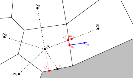
Figure 1: Part of an unstructured grid, showing cell $P$ and its neighbouring cells, each having a single common face with $P$. The shaded area lies outside the grid. The faces and neighbours of cell $P$ are numbered in anticlockwise order, with face $f$ separating $P$ from its neighbour $N_{f}$. The geometric characteristics of its face 1 which separates it from neighbouring cell $N_{1}$ are displayed. The position vectors of the centroids of cells $P$ and $N_{f}$ are denoted by the same characters but in boldface as $\bm{P}$ and $\bm{N}_{f}$; $\bm{c}_{f}$ is the centroid of face $f$ and $\bm{c}^{\prime}_{f}$ is its closest point on the line segment connecting $\bm{P}$ and $\bm{N}_{f}$; $\bm{m}_{f}$ is the midpoint between $\bm{P}$ and $\bm{N}_{f}$; $\bm{n}_{f}$ is the unit vector normal to face $f$, pointing outwards of $P$. The shown cell $P$ also has a boundary face (face 5), with no neighbour on the other side; in this case $\bm{c}^{\prime}_{5}$ is the projection of $\bm{P}$ onto the boundary face.

Our goal is to derive approximate algebraic gradient operators $\nabla^{\mathrm{a}}$ which return values $\nabla^{\mathrm{a}}\phi(\bm{P})\approx\nabla\phi(\bm{P})$ at each cell centroid $\bm{P}$, using information only from the immediate neighbouring cells and boundary faces. The components of the approximate gradient are denoted as $\nabla^{\mathrm{a}}\phi=(\phi_{\!.x}^{\mathrm{a}},\phi_{\!.y}^{\mathrm{a}})$. The operators $\nabla^{\mathrm{a}}$ must be capable of approximating the derivative on grids of arbitrary geometry. To study the effect of grid geometry on the accuracy, we must define some indicators of grid irregularity. With the present grid arrangement, we find it useful to define three kinds of such grid irregularities, which we shall call here “non-orthogonality”, “unevenness” and “skewness” (other possibilities exist, see e.g. [23]). We will define these terms with the aid of Fig. 1. With the nomenclature defined in that figure, we will say that face $f$ of cell $P$ exhibits non-orthogonality if $\bm{N}_{f}-\bm{P}$ is not parallel to $\bm{n}_{f}$; a measure of non-orthogonality is the angle between the vectors $(\bm{N}_{f}-\bm{P})$ and $\bm{n}_{f}$. Also, we will say that face $f$ exhibits unevenness if the midpoint of the line segment joining $\bm{P}$ and $\bm{N}_{f}$, $\bm{m}_{f}=(\bm{P}+\bm{N}_{f})/2$, does not coincide with $\bm{c}^{\prime}_{f}$ (i.e. the cell centres are unequally spaced on either side of the face); a measure of unevenness is $\|\bm{c}^{\prime}_{f}-\bm{m}_{f}\|/\|\bm{N}_{f}-\bm{P}\|$. Finally, we will say that face $f$ exhibits skewness if $\bm{c}^{\prime}_{f}$ does not coincide with $\bm{c}_{f}$ (i.e. the line joining the cell centres does not pass through the centre of the face); a measure of the skewness is $\|\bm{c}_{f}-\bm{c}^{\prime}_{f}\|/\|\bm{N}_{f}-\bm{P}\|$.

Before discussing the DT and LS gradient schemes, it is useful to examine a simpler scheme which is applicable on very plain grids that are formed from two families of equispaced parallel straight lines intersecting at a constant angle, as in Fig. 2. In this case all the cells of the grid are identical parallelograms (Cartesian grids with constant spacing are a special case of this category). Figure 2 shows a cell $P$ belonging to such a grid, and its four neighbouring cells. The vectors $\bm{\delta}^{\xi}$ and $\bm{\delta}^{\eta}$ are parallel to the grid lines and span the size of the cells. Due to the grid properties it holds that $\bm{\delta}^{\xi}=\bm{c}_{1}-\bm{c}_{3}=\bm{N}_{1}-\bm{P}=\bm{P}-\bm{N}_{3}$ and $\bm{\delta}^{\eta}=\bm{c}_{2}-\bm{c}_{4}=\bm{N}_{2}-\bm{P}=\bm{P}-\bm{N}_{4}$. It can be assumed that two variables, $\xi$ and $\eta$, are distributed in the domain, such that in the direction of $\bm{\delta}^{\xi}$ the variable $\xi$ varies linearly while $\eta$ is constant, and in the direction of $\bm{\delta}^{\eta}$ the variable $\eta$ varies linearly while $\xi$ is constant. Then the grid can be considered to be constructed by drawing lines of constant $\xi$ and of constant $\eta$, equispaced (in the $\xi,\eta$ space) by $\Delta\xi$ and $\Delta\eta$, respectively. Let us assume also that the grid density can be increased by adjusting the spacings $\Delta\xi$ and $\Delta\eta$, but their ratio must be kept constant, e.g. if $\Delta\xi=h$ then $\Delta\eta=\alpha h$ with $\alpha$ being a constant, independent of $h$. The variable $h$ determines the grid fineness. Therefore, the direction of the grid vectors $\bm{\delta}^{\xi}$ and $\bm{\delta}^{\eta}$ remains constant with grid refinement, but their lengths are proportional to the grid parameter $h$.

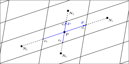
Figure 2: Part of a grid formed by equispaced parallel grid lines. See the text for details.

This idealized grid exhibits no unevenness or skewness. It possibly exhibits non-orthogonality, but this poses no problem as far as the gradient calculation is concerned. Since points $\bm{N}_{3}$, $\bm{P}$ and $\bm{N}_{1}$ are collinear and equidistant, the rate of change of any quantity $\phi$ in the direction of $\bm{\delta}^{\xi}$ can be approximated at point $\bm{P}$ from the values at $\bm{N}_{3}$ and $\bm{N}_{1}$ using second-order accurate central differencing. In the same manner, the rate of change in the direction of $\bm{\delta}^{\eta}$ at $\bm{P}$ can be approximated from the values at $\bm{N}_{4}$ and $\bm{N}_{2}$. So, let the grid vectors be written in Cartesian coordinates as $\bm{\delta}^{\xi}=(\delta^{\xi}_{x},\delta^{\xi}_{y})$ and $\bm{\delta}^{\eta}=(\delta^{\eta}_{x},\delta^{\eta}_{y})$, respectively. Then, by expanding the function $\phi$ in a two-dimensional Taylor series along the Cartesian directions, centred at point $\bm{P}$, and using that to express the values at the points $\bm{N}_{1}=\bm{P}+\bm{\delta}^{\xi}$, $\bm{N}_{3}=\bm{P}-\bm{\delta}^{\xi}$, $\bm{N}_{2}=\bm{P}+\bm{\delta}^{\eta}$ and $\bm{N}_{4}=\bm{P}-\bm{\delta}^{\eta}$ we get

$$\phi(\bm{N}_{1})-\phi(\bm{N}_{3}) =\nabla\phi(\bm{P})\cdot(2\bm{\delta}^{\xi})\;+\;O(h^{3})$$

$$\phi(\bm{N}_{2})-\phi(\bm{N}_{4}) =\nabla\phi(\bm{P})\cdot(2\bm{\delta}^{\eta})\;+\;O(h^{3})$$

This system can be solved for $\nabla\phi(\bm{P})\equiv(\phi_{\!.x},\phi_{\!.y})$ to get

$$\begin{bmatrix}\phi_{\!.x}(\bm{P})\\[4.26773pt] \phi_{\!.y}(\bm{P})\end{bmatrix}\;=\quad\frac{1}{2\Omega_{P}}\left[\begin{array}[]{rr}\delta_{y}^{\eta}&-\delta_{y}^{\xi}\\[4.26773pt] -\delta_{x}^{\eta}&\delta_{x}^{\xi}\end{array}\right]\!\cdot\!\begin{bmatrix}\phi(\bm{N}_{1})-\phi(\bm{N}_{3})\\[4.26773pt] \phi(\bm{N}_{2})-\phi(\bm{N}_{4})\end{bmatrix}\quad+\quad\frac{1}{2\Omega_{P}}\left[\begin{array}[]{rr}\delta_{y}^{\eta}&-\delta_{y}^{\xi}\\[4.26773pt] -\delta_{x}^{\eta}&\delta_{x}^{\xi}\end{array}\right]\!\cdot\!\begin{bmatrix}O(h^{3})\\[4.26773pt] O(h^{3})\end{bmatrix}$$

where $\Omega_{P}=\delta_{x}^{\xi}\delta_{y}^{\eta}-\delta_{y}^{\xi}\delta_{x}^{\eta}=\|\bm{\delta}^{\xi}\times\bm{\delta}^{\eta}\|$ is the volume (area in 2D) of cell $P$. The last term in the above equation, involving the unknown $O(h^{3})$ terms, is of order $O(h^{2})$ because $\Omega_{P}=O(h^{2})$ and all the $\delta$’s are $O(h)$. So, carrying out the matrix multiplications we arrive at

$$\nabla\phi(\bm{P})\;\equiv\;\begin{bmatrix}\phi_{\!.x}(\bm{P})\\[4.26773pt] \phi_{\!.y}(\bm{P})\end{bmatrix}\;=\;\underbrace{\frac{1}{2\Omega_{P}}\begin{bmatrix}\delta_{y}^{\eta}(\phi(\bm{N}_{1})\!-\!\phi(\bm{N}_{3}))\,-\,\delta_{y}^{\xi}(\phi(\bm{N}_{2})\!-\!\phi(\bm{N}_{4}))\\[4.26773pt] \delta_{x}^{\xi}(\phi(\bm{N}_{2})\!-\!\phi(\bm{N}_{4}))\,-\,\delta_{x}^{\eta}(\phi(\bm{N}_{1})\!-\!\phi(\bm{N}_{3}))\end{bmatrix}}_{\nabla^{\mathrm{s}}\phi(\bm{P})}\;+\;\begin{bmatrix}O(h^{2})\\[4.26773pt] O(h^{2})\end{bmatrix}$$ (1)

Finally, we drop the unknown $O(h^{2})$ terms in Eq. (1) and are left with a second-order approximation to the gradient, $\nabla^{\mathrm{s}}$; the dropped terms are called the truncation error of the operator $\nabla^{\mathrm{s}}$. The fact that this formula has been derived for a grid constructed from equidistant parallel lines may seem too restrictive, but in fact the utility of Eq. (1) goes beyond this narrow context, as will now be explained.

Consider again structured grid generation based on a pair of variables $\xi$, $\eta$ distributed smoothly in the domain, where curves of constant $\xi$ and $\eta$ are drawn at equal intervals of $\Delta\xi$ and $\Delta\eta$, respectively. This time $\xi$ and $\eta$ are not required to vary linearly nor to be constant along straight lines. Therefore, a curvilinear grid such as that shown in Fig. 3 may result, constructed by joining the points of intersection of these two families of curves by straight line segments (the dashed lines in Fig. 3).

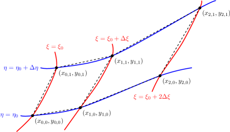
Figure 3: Part of a grid (dashed straight lines) constructed from lines of constant $\xi$ (red curves) and $\eta$ (blue curves), where $\xi$, $\eta$ are variables distributed smoothly in the domain. The lines are equispaced with constant spacings $\Delta\xi$ and $\Delta\eta$, respectively. Grid node $(i,j)$ is located at $(\xi_{i},\eta_{j})=(\xi_{0}+i\,\Delta\xi,\eta_{0}+j\,\Delta\eta)$ in the computational space, where $(\xi_{0},\eta_{0})$ is a predefined point, and at $(x_{i,j},y_{i,j})$ in the physical space.

There is a one-to-one correspondence of coordinates $(x,y)$ of the physical space to coordinates $(\xi,\eta)$ of the computational space. Therefore, not only are the computational coordinates functions of the physical coordinates ($\xi=\xi(x,y)$ and $\eta=\eta(x,y)$), but the physical coordinates $(x,y)$ can also be regarded as functions of the computational coordinates ($x=x(\xi,\eta)$ and $y=y(\xi,\eta)$). Since the latter vary smoothly in the domain, $(x,y)$ can be expanded in Taylor series around a reference point $(\xi_{0},\eta_{0})$. For example, for the $x$ coordinate,

$$x(\xi_{0}+\delta\xi,\eta_{0}+\delta\eta)\;=\;x(\xi_{0},\eta_{0})\;+\;x_{\!.\xi}\delta\xi\;+\;x_{\!.\eta}\delta\eta\;+\;O(h^{2})$$ (2)

where the derivatives are evaluated at point $(\xi_{0},\eta_{0})$. In this way, we can express the coordinates of all the grid vertices $(x_{i,j},y_{i,j})$ shown in Fig. 3 as functions of $(x_{0,0},y_{0,0})\equiv(x(\xi_{0},\eta_{0}),y(\xi_{0},\eta_{0}))$ and of the derivatives $x_{.\xi}$ etc. there. Using these expansions, it is easy to show that

$$\lim_{\Delta\xi,\Delta\eta\rightarrow 0}\left(\frac{x_{1,1}-x_{1,0}}{x_{0,1}-x_{0,0}}\right)\;=\;\lim_{\Delta\xi,\Delta\eta\rightarrow 0}\left(\frac{y_{1,1}-y_{1,0}}{y_{0,1}-y_{0,0}}\right)\;=\;1$$ (3)

and

$$\lim_{\Delta\xi,\Delta\eta\rightarrow 0}\left(\frac{x_{2,0}-x_{1,0}}{x_{1,0}-x_{0,0}}\right)\;=\;\lim_{\Delta\xi,\Delta\eta\rightarrow 0}\left(\frac{y_{2,0}-y_{1,0}}{y_{1,0}-y_{0,0}}\right)\;=\;1$$ (4)

Equation (3) implies that, as the grid is refined by reducing the $\Delta\xi$, $\Delta\eta$ spacings, neighbouring grid lines of the same family become more and more parallel, so that grid skewness tends to zero. Equation (4) implies that, as the grid is refined, neighbouring cells tend to become of equal size, so that grid unevenness tends to zero. The conclusion is that on structured grids which are constructed from smooth distributions of auxiliary variables $(\xi,\eta)$, grid refinement causes the geometry of a cell and its neighbours to locally approach that depicted in Fig. 2. This has an important consequence: any numerical scheme for computing the gradient that reduces to Eq. (1) on parallelogram grids (such as that of Fig. 2) is of second-order accuracy on smooth structured grids (such as that of Fig. 3). It so happens that both the DT scheme and the LS scheme belong to this category. Unfortunately, grid refinement does not engender such a quality improvement when it comes to unstructured meshes.

3 Gradient calculation using the divergence theorem

For grids of more general geometry, like that of Fig. 1, a more general method is needed. Let $\Omega_{P}$ denote the volume of cell $P$ and $S_{P}$ its bounding surface. The DT gradient scheme is based on a derivative of the divergence theorem, which can be expressed as follows:

$$\int_{\Omega_{P}}\nabla\phi\,\mathrm{d}\Omega\;=\;\int_{S_{P}}\phi\,\bm{n}\,\mathrm{d}s$$

where $\bm{n}$ is the unit vector perpendicular to $S_{P}$ at each point, pointing outwards of the cell, while $\mathrm{d}\Omega$ and $\mathrm{d}s$ are infinitesimal elements of the volume and surface, respectively. The bounding surface $S_{P}$ can be decomposed into $F$ faces which are denoted by $S_{f}$, $f=1,\ldots,F$ ($F=5$ in Fig. 1). These faces are assumed to be straight (planar, in 3 dimensions), as in Fig. 1, so that the normal unit vector $\bm{n}$ has a constant value $\bm{n}_{f}$ along each face $f$. Therefore, the above equation can be written as

$$\int_{\Omega_{P}}\nabla\phi\,\mathrm{d}\Omega\;=\;\sum_{f=1}^{F}\left(\bm{n}_{f}\int_{S_{f}}\phi\,\mathrm{d}s\right)$$ (5)

According to the midpoint integration rule [1, 24], the mean value of a quantity over cell $P$ (or face $f$) is equal to its value at the centroid $\bm{P}$ of the cell (or $\bm{c}_{f}$ of the face), plus a second-order correction term. Applying this to the mean values of $\nabla\phi$ and $\phi$ over $\Omega_{P}$ and $S_{f}$ we get, respectively:

$$\frac{1}{\Omega_{P}}\int_{\Omega_{P}}\nabla\phi\,\mathrm{d}\Omega\;=\;\nabla\phi(\bm{P})\;+\;\bm{O}(h^{2})\;\Rightarrow\quad\int_{\Omega_{P}}\nabla\phi\,\mathrm{d}\Omega\;=\;\nabla\phi(\bm{P})\,\Omega_{P}\;+\;\bm{O}(h^{4})$$ (6)

$$\frac{1}{S_{f}}\int_{S_{f}}\phi\,\mathrm{d}s\;=\;\phi(\bm{c}_{f})\;+\;O(h^{2})\;\Rightarrow\quad\int_{S_{f}}\phi\,\mathrm{d}s\;=\;\phi(\bm{c}_{f})\,S_{f}\;+\;O(h^{3})$$ (7)

where $h$ is a characteristic grid spacing (we used that $\Omega_{P}=O(h^{2})$ and $S_{f}=O(h)$). Substituting these expressions into the divergence theorem, Eq. (5), we get

$$\nabla\phi(\bm{P})\;=\;\frac{1}{\Omega_{P}}\sum_{f=1}^{F}\phi(\bm{c}_{f})\,S_{f}\,\bm{n}_{f}\;+\;\bm{O}(h)$$ (8)

The above formula is exact as long as the unknown $\bm{O}(h)$ term is retained, which consists mostly of face contributions arising from Eq. (7), whereas the volume contribution from Eq. (6) is only $\bm{O}(h^{2})$. Dropping this term would leave us with a first-order accurate approximation. However, this approximation cannot be the final formula for the gradient because Eq. (8) contains $\phi(\bm{c}_{f})$, the $\phi$ values at the face centres, whereas we need a formula that uses only the values at the cell centres. The common practice is to approximate $\phi(\bm{c}_{f})$ by $\phi(\bm{c}^{\prime}_{f})$, the exact values of $\phi$ at points $\bm{c}^{\prime}_{f}$ rather than $\bm{c}_{f}$ (see Fig. 1); these values also do not belong to the set of cell-centre values, but since $\bm{c}^{\prime}_{f}$ lies on the line segment joining cell centres $\bm{P}$ and $\bm{N}_{f}$, the value $\phi(\bm{c}^{\prime}_{f})$ can in turn be approximated by linear interpolation between $\phi(\bm{P})$ and $\phi(\bm{N}_{f})$, say $\bar{\phi}(\bm{c}^{\prime}_{f})$ (the overbar denotes linear interpolation):

$$\bar{\phi}(\bm{c}^{\prime}_{f})\;\equiv\;\frac{\|\bm{c}^{\prime}_{f}-\bm{N}_{f}\|}{\|\bm{N}_{f}-\bm{P}\|}\,\phi(\bm{P})\;+\;\frac{\|\bm{c}^{\prime}_{f}-\bm{P}\|}{\|\bm{N}_{f}-\bm{P}\|}\,\phi(\bm{N}_{f})\;=\;\phi(\bm{c}^{\prime}_{f})\;+\;O(h^{2})$$ (9)

Linear interpolation is known to be second-order accurate, hence the $O(h^{2})$ term in the above equation. Thus, by using $\bar{\phi}(\bm{c}^{\prime}_{f})$ instead of $\phi(\bm{c}_{f})$ in the right hand side of Eq. (8) and dropping the unknown $\bm{O}(h)$ term we obtain an approximation to the gradient which depends only on cell-centre values of $\phi$:

$$\nabla^{\mathrm{d}0}\phi(\bm{P})\;\equiv\;\frac{1}{\Omega_{P}}\sum_{f=1}^{F}\bar{\phi}(\bm{c}^{\prime}_{f})\,S_{f}\,\bm{n}_{f}$$ (10)

This is called the “divergence theorem” (DT) gradient. It applies in both two and three dimensions.

An important question is whether and how the replacement of $\phi(\bm{c}_{f})$ by $\bar{\phi}(\bm{c}^{\prime}_{f})$, that led from Eq. (8) to the formula (10), has affected the accuracy. To answer this question we first need to deduce how much $\bar{\phi}(\bm{c}^{\prime}_{f})$ differs from $\phi(\bm{c}_{f})$. This can be done by using the exact $\phi(\bm{c}^{\prime}_{f})$ as an intermediate value. We will consider structured grids and unstructured grids separately.

Structured grids

As discussed in the previous Section, the skewness of smooth structured grids diminishes with refinement, and in fact expressing the points involved in its definition as Taylor series of the form (2) it can be shown that $\|\bm{c}_{f}-\bm{c}^{\prime}_{f}\|/\|\bm{N}_{f}-\bm{P}\|=O(h)$, or $\bm{c}_{f}-\bm{c}^{\prime}_{f}=\bm{O}(h^{2})$. Therefore, expanding $\phi(\bm{c}_{f})$ in a Taylor series about point $\bm{c}^{\prime}_{f}$ gives $\phi(\bm{c}_{f})=\phi(\bm{c}^{\prime}_{f})+\nabla\phi(\bm{c}^{\prime}_{f})\cdot(\bm{c}_{f}-\bm{c}^{\prime}_{f})+O(h^{2})=\phi(\bm{c}^{\prime}_{f})+O(h^{2})$. Next, $\phi(\bm{c}^{\prime}_{f})$ can be expressed in terms of $\bar{\phi}(\bm{c}^{\prime}_{f})$ according to Eq. (9). Putting everything together results in the sought relationship:

$$\phi(\bm{c}_{f})\;=\;\phi(\bm{c}^{\prime}_{f})+O(h^{2})\;=\;(\bar{\phi}(\bm{c}^{\prime}_{f})+O(h^{2}))+O(h^{2})\;=\;\bar{\phi}(\bm{c}^{\prime}_{f})+O(h^{2})$$ (11)

Substituting this into Eq. (8), and considering that $\Omega_{P}=O(h^{2})$ and $S_{f}=O(h)$, we arrive at

$$\nabla\phi(\bm{P})\;=\;\frac{1}{\Omega_{P}}\sum_{f=1}^{F}\bar{\phi}(\bm{c}^{\prime}_{f})\,S_{f}\,\bm{n}_{f}\;+\;\bm{O}(h)$$ (12)

The first term on its right-hand side is just the approximate gradient $\nabla^{\mathrm{d0}}$, Eq. (10). Therefore, the truncation error of $\nabla^{\mathrm{d0}}$ is $\bm{\tau}\equiv\nabla^{\mathrm{d}0}\phi(\bm{P})-\nabla\phi(\bm{P})=\bm{O}(h)$. Actually, the situation is even better because the leading terms of the contributions of opposite faces to the $\bm{O}(h)$ term in Eq. (12) cancel out leaving a net $\bm{O}(h^{2})$ truncation error, making the method second-order accurate. The proof is tedious and involves writing analytic expressions for the truncation error contributions of each face; it can be performed more easily for a grid such as that shown in Fig. 2 where the divergence theorem procedure described in the present Section is an alternative path to arrive at the exact same formula, Eq. (1), $\nabla^{\mathrm{d}0}\equiv\nabla^{\mathrm{s}}$, with its $\bm{O}(h^{2})$ truncation error.

The error cancellation between opposite faces does not always occur; sometimes the worst-case scenario of $\bm{O}(h)$ truncation error predicted by Eq. (12) holds. An example is at boundary cells. Fig. 4 shows a boundary cell $P$ belonging to a Cartesian grid which exhibits neither skewness nor unevenness (in fact, it does not even exhibit non-orthogonality). Yet cell $P$ has no neighbour on the boundary side, and so the centre of its boundary face, $\bm{c}_{3}$, is used instead of a neighbouring cell centre. This introduces “unevenness” in the $x$- (horizontal) direction because the distances $\|\bm{N}_{1}-\bm{P}\|=h$ and $\|\bm{c}_{3}-\bm{P}\|=h/2$ are not equal. The $x$- component of the divergence theorem gradient (10) reduces to

$$\phi_{\!.x}^{\mathrm{d}0}(\bm{P})\;=\;\frac{1}{2h}\left(\phi(\bm{N}_{1})+\phi(\bm{P})-2\phi(\bm{c}_{3})\right)$$ (13)

which is only first-order accurate, since expanding $\phi(\bm{N}_{1})$ and $\phi(\bm{c}_{3})$ in Taylor series about $\bm{P}$ gives

$$\phi_{\!.x}^{\mathrm{d}0}(\bm{P})\;=\;\phi_{\!.x}(\bm{P})\;+\;\frac{1}{8}\phi_{\!.xx}(\bm{P})\,h\;+\;O(h^{2})$$

This offers a nice demonstration of the effect of error cancellation between opposite faces. Equation (10) is obtained from Eq. (8) by using interpolated values $\bar{\phi}(\bm{c}^{\prime}_{f})$ instead of the exact but unknown values $\phi(\bm{c}_{f})$ at the face centres. Therefore, one might expect that since the cell of Fig. 4 has a boundary face and the exact value at its centre, $\phi(\bm{c}_{3})$, is used rather than an interpolated value, the result would be more accurate; but the above analysis shows exactly the opposite: the error increases from $O(h^{2})$ to $O(h)$. This is due to the fact that by dropping the interpolation error on the boundary face the corresponding error on the opposite face $1$ is no longer counterbalanced.

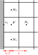
Figure 4: A boundary cell $P$ belonging to a Cartesian grid.

Another example where error cancellation does not occur and the formal $\bm{O}(h)$ accuracy predicted by Eq. (12) holds is the common case of grid that consists of triangles that come from dividing each cell of a smooth structured grid along the same diagonal. For example, application of this procedure to the grid shown in Fig. 2 results in the grid of Fig. 5. The latter may be seen to exhibit neither unevenness nor skewness as the face centres $\bm{c}_{f}$ coincide with the midpoints of the line segments joining cell centre $\bm{P}$ to its neighbours $\bm{N}_{f}$. Thus Eq. (11) holds, leading to Eq. (12). This time, however, a tedious but straightforward calculation where neighbouring $\phi(\bm{N}_{f})$ values are expressed in Taylor series about $\bm{P}$ and substituted in (12) shows that there is no cancellation and the truncation error remains $\bm{O}(h)$. If the grid comes from triangulation of a curvilinear structured grid (Fig. 3) then the skewness is not zero but it diminishes with refinement at an $O(h)$ rate (Eq. (11)) and exactly the same conclusions hold.

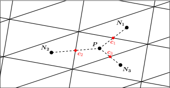
Figure 5: Grid of triangles constructed through bisection of the cells of the structured grid of Fig. 2 along their same diagonal.

In fact, from the considerations leading to Eq. (11) it follows that if a grid generation algorithm is such that skewness diminishes as $O(h^{p})$ then the order of accuracy of the DT gradient is at least $\min\{p,1\}$.

Unstructured grids

Unstructured grids usually consist of triangles (or tetrahedra in 3D), or of polygonal (polyhedral in 3D) cells which are also formed by a triangulation process. They are typically constructed using algorithms that are based on geometrical principles that do not depend on grid fineness, so that there is some self-similarity between coarse and fine grids and refinement does not reduce the skewness, i.e. $\|\bm{c}_{f}-\bm{c}^{\prime}_{f}\|/\|\bm{N}_{f}-\bm{P}\|=O(1)$. This means that $\bm{c}_{f}-\bm{c}^{\prime}_{f}=\bm{O}(h)$ and therefore instead of Eq. (11) we now have

$$\phi(\bm{c}_{f})\;=\;\phi(\bm{c}^{\prime}_{f})+O(h)\;=\;(\bar{\phi}(\bm{c}^{\prime}_{f})+O(h^{2}))+O(h)\;=\;\bar{\phi}(\bm{c}^{\prime}_{f})+O(h)$$ (14)

Substituting this into the exact equation (8) we get

$$\nabla\phi(\bm{P})\; =\;\frac{1}{\Omega_{P}}\sum_{f=1}^{F}\left(\bar{\phi}(\bm{c}^{\prime}_{f})+O(h)\right)\,S_{f}\,\bm{n}_{f}\;+\;\bm{O}(h)$$

$$=\;\frac{1}{\Omega_{P}}\sum_{f=1}^{F}\bar{\phi}(\bm{c}^{\prime}_{f})\,S_{f}\,\bm{n}_{f}\;+\;\frac{1}{\Omega_{P}}\sum_{f=1}^{F}O(h)\,S_{f}\,\bm{n}_{f}\;+\;\bm{O}(h)$$

which, considering that $\Omega_{P}=O(h^{2})$ and $S_{f}=O(h)$, means that

$$\nabla\phi(\bm{P})\;=\;\frac{1}{\Omega_{P}}\sum_{f=1}^{F}\bar{\phi}(\bm{c}^{\prime}_{f})\,S_{f}\,\bm{n}_{f}\;+\;\bm{O}(1)\;+\;\bm{O}(h)$$ (15)

Again, the first term on its right-hand side is the approximate gradient $\nabla^{\mathrm{d0}}$, Eq. (10). But this time, unlike in the structured grid case, the truncation error of $\nabla^{\mathrm{d0}}$ is $\bm{\tau}\equiv\nabla^{\mathrm{d}0}\phi(\bm{P})-\nabla\phi(\bm{P})=\bm{O}(1)$. Nor do the leading terms of the face contributions to the truncation error cancel out to increase its order, because on unstructured grids the orientations and sizes of the faces are unrelated. This is an unfortunate result, because it means that the approximation (10) is zeroth-order accurate, as the error $\bm{O}(1)$ does not decrease with grid refinement, but instead $\nabla^{\mathrm{d}0}\phi(\bm{P})$ converges to a value that is not equal to $\nabla\phi(\bm{P})$ (see Section 5.4 for an example).

Acknowledging that the lack of accuracy is due to the bad representation of the $\phi(\bm{c}_{f})$ values in Eq. (8) by $\bar{\phi}(\bm{c}^{\prime}_{f})$, application of the formula (10) is often followed by a “corrector step” where, instead of the values $\bar{\phi}(\bm{c}^{\prime}_{f})$, the “improved” values $\hat{\phi}(\bm{c}_{f})$ are used, defined as

$$\hat{\phi}(\bm{c}_{f})\;\equiv\;\bar{\phi}(\bm{c}^{\prime}_{f})\;+\;\overline{\nabla^{\mathrm{d}0}\phi}(\bm{c}^{\prime}_{f})\!\cdot\!(\bm{c}_{f}-\bm{c}^{\prime}_{f})$$ (16)

where $\overline{\nabla^{\mathrm{d}0}\phi}(\bm{c}^{\prime}_{f})$ is obtained by linear interpolation (Eq. (9)) between $\nabla^{\mathrm{d}0}\phi(\bm{P})$ and $\nabla^{\mathrm{d}0}\phi(\bm{N}_{f})$ at point $\bm{c}^{\prime}$ (these were calculated in the previous step (10), the “predictor” step). This results in an approximation which is hopefully more accurate than (10):

$$\nabla^{\mathrm{d}1}\phi(\bm{P})\;\equiv\;\frac{1}{\Omega_{P}}\sum_{f=1}^{F}\hat{\phi}(\bm{c}_{f})\,S_{f}\,\bm{n}_{f}$$ (17)

The values $\hat{\phi}(\bm{c}_{f})$ are expected to be better approximations to $\phi(\bm{c}_{f})$ than $\bar{\phi}(\bm{c}^{\prime}_{f})$ are, because Eq. (16) tries to account for skewness by mimicking the Taylor series expansion

$$\phi(\bm{c}_{f})\;=\;\phi(\bm{c}^{\prime}_{f})\;+\;\nabla\phi(\bm{c}^{\prime}_{f})\cdot(\bm{c}_{f}-\bm{c}^{\prime}_{f})\;+\;O(h^{2})$$ (18)

Unfortunately, since in Eq. (16) only a crude approximation of $\nabla\phi(\bm{c}^{\prime}_{f})$ is used, namely $\overline{\nabla^{\mathrm{d}0}\phi}(\bm{c}^{\prime}_{f})=\nabla\phi(\bm{c}^{\prime}_{f})+\bm{O}(1)$, what we get by subtracting Eq. (16) from Eq. (18) is $\hat{\phi}(\bm{c}_{f})=\phi(\bm{c}_{f})+O(h)$ which may have greater accuracy but not greater order of accuracy than the previous estimate $\bar{\phi}(\bm{c}^{\prime}_{f})=\phi(\bm{c}_{f})+O(h)$, Eq. (14). Substituting this into Eq. (8) we arrive again at an equation similar to (15) which shows that the error of the approximation (17) is also of order $\bm{O}(1)$.

Further correction steps may be applied in the same manner; a fixed finite number of such steps may increase the accuracy, but the order of accuracy with respect to grid refinement will remain zero. But if this procedure is repeated until convergence to an operator $\nabla^{{\mathrm{d}}\infty}$, say, then $\nabla^{{\mathrm{d}}\infty}$ would simultaneously satisfy both Eqs. (16) and (17), or combined in a single equation:

$$\nabla^{\mathrm{d}\infty}\phi(\bm{P})\;-\;\frac{1}{\Omega_{P}}\sum_{f=1}^{F}\overline{\nabla^{\mathrm{d}\infty}\phi}(\bm{c}^{\prime}_{f})\!\cdot\!(\bm{c}_{f}-\bm{c}^{\prime}_{f})\,S_{f}\,\bm{n}_{f}\;=\;\frac{1}{\Omega_{P}}\sum_{f=1}^{F}\bar{\phi}(\bm{c}^{\prime}_{f})\,S_{f}\,\bm{n}_{f}$$ (19)

where we have moved all terms involving the gradient to the left-hand side. An analogous equation can be derived for the exact gradient, from Eqs. (8), (18), and (9):

$$\nabla\phi(\bm{P})\;-\;\frac{1}{\Omega_{P}}\sum_{f=1}^{F}\overline{\nabla\phi}(\bm{c}^{\prime}_{f})\!\cdot\!(\bm{c}_{f}-\bm{c}^{\prime}_{f})\,S_{f}\,\bm{n}_{f}\;=\;\frac{1}{\Omega_{P}}\sum_{f=1}^{F}\bar{\phi}(\bm{c}^{\prime}_{f})\,S_{f}\,\bm{n}_{f}\;+\;\bm{O}(h)$$ (20)

By subtracting Eq. (20) from Eq. (19) we get an expression for the truncation error $\bm{\tau}\equiv\nabla^{\mathrm{d}\infty}\phi-\nabla\phi$:

$$\bm{\tau}(\bm{P})\;-\;\frac{1}{\Omega_{P}}\sum_{f=1}^{F}\overline{\bm{\tau}}(\bm{c}^{\prime}_{f})\!\cdot\!(\bm{c}_{f}-\bm{c}^{\prime}_{f})\,S_{f}\,\bm{n}_{f}\;=\;\bm{O}(h)$$ (21)

The left-hand side is a linear combination of not only $\bm{\tau}(\bm{P})$ but also $\bm{\tau}(\bm{N}_{f})$ at all neighbour points. Since $\Omega_{P}=O(h^{2})$, $S_{f}=O(h)$ and $\bm{c}_{f}-\bm{c}^{\prime}_{f}=O(h)$, the coefficients of this linear combination are $O(1)$ i.e. they do not depend on the grid fineness but only on the grid geometry (skewness, unevenness etc.). Expression (21) suggests that $\bm{\tau}=\bm{O}(h)$, i.e. that $\nabla^{\mathrm{d}\infty}$ is first-order accurate, although to ascertain this one would have to assemble Eqs. (21) for all grid cells in a large linear system $A\tau=b\Rightarrow\tau=A^{-1}b$ (where $\tau$ stores the $x$- and $y$- (and $z$-, in 3D) components of $\bm{\tau}$ at all cell centres and $b=O(h)$), select a suitable matrix norm $\|\cdot\|$, and ensure that $\|A^{-1}\|$ remains bounded as $h\rightarrow 0$.

So, iterating Eqs. (16) and (17) until convergence one would hope that a first-order accurate gradient $\nabla^{\mathrm{d}\infty}$ would be obtained. As reported in [19], convergence of this procedure is not guaranteed and underrelaxation may be needed, leading to a large number of required iterations and great computational cost. In practice, the desired accuracy will be reached with a finite number of iterations, but this number is not known a priori and must be determined by trials; furthermore, in order to maintain the property that grid refinement improves the accuracy, the number of iterations should increase with grid refinement in order to avoid accuracy stagnation. Considering that the main rival of the DT gradient, the LS gradient, costs approximately as much as the DT gradient with a single corrector step (see Sec. 6.1), it can be seen that this iterative procedure is impractical and may end up consuming most of the computational time of a FVM solver. Alternatively, one could directly solve all the equations (19) simultaneously in a large linear system; this is also proposed and tested in [19], along with a second-order accurate method that additionally computes the Hessian matrix. Obviously, this approach also involves a very large computational cost.

However, we would like to propose here a way to avoid the extra cost of the iterative procedure for the gradient. The FVM generally employs outer iterations to solve a PDE (e.g. SIMPLE iterations, as opposed to the inner iterations of the linear solvers employed). Outer iterations are necessary when the equations solved are non-linear, but may be used also when solving linear problems if some terms are treated with the deferred-correction approach. FVMs that use gradient schemes such as those presently discussed are almost always iterative, with the gradients computed using the values of the dependent variable from the previous outer iteration. The idea is then to exploit these outer iterations, dividing the “gradient iterations” among them: at each outer iteration $n$ a single “gradient iteration” is performed according to

$$\nabla^{\mathrm{d}n}\phi(\bm{P})\;=\;\frac{1}{\Omega_{P}}\sum_{f=1}^{F}\left(\overline{\phi^{n-1}}(\bm{c}^{\prime}_{f})\;+\;\overline{\nabla^{\mathrm{d}(n-1)}\phi}(\bm{c}^{\prime}_{f})\!\cdot\!(\bm{c}_{f}-\bm{c}^{\prime}_{f})\right)\,S_{f}\,\bm{n}_{f}$$ (22)

which means that one has to store not only the solution of the previous outer iteration $\phi^{n-1}$ but also the gradient of that iteration $\nabla^{\mathrm{d}(n-1)}\phi$, which many codes do already. Since only one calculation is performed per outer iteration, the cost of this procedure is almost as low as that of the uncorrected DT gradient (10), but it converges to the first-order accurate $\nabla^{\mathrm{d}\infty}$ gradient operator instead of the zeroth-order accurate $\nabla^{\mathrm{d}0}$. For explicit time-dependent FVM methods, Eq. (22) could be applied with $n-1$ denoting the previous time step; in the very first time step it may be necessary to perform several “gradient iterations” to obtain a consistent gradient to begin with.

Iterative schemes that are different from (22) can also be devised; a similar iterative technique is used in [25] in order to determine the coefficients of reconstruction polynomials without solving large linear systems. There, Jacobi, Gauss-Seidel, and SOR-type iterations are applied, with the latter found to be the most efficient. The present scheme (22) is reminiscent of the Jacobi iterative procedure (although not exactly equivalent, since $\nabla\phi(\bm{P})$ appears also at the right-hand side, within the averaged gradient, evaluated from the previous iteration). A scheme reminiscent of the Gauss-Seidel iterative procedure would be one where in the right-hand side of Eq. (22) new values of the gradient at neighbour cells (calculated at the current outer iteration) are used whenever available instead of using the old values. However, in the present work only the scheme (22) is tested in Section 6.1.

At this point we would like to make a brief comment concerning the calculation of the gradient at boundary cells. The above analysis has assumed that at boundary faces the values of $\phi$ at the face centres are available. However, this is not always the case; in situations where these values are not available, they must be approximated to at least second-order accuracy as otherwise the DT gradient will be inconsistent, as the preceding analysis has shown. For example, in problems with Neumann boundary conditions the directional derivative normal to the boundary, $g$ say, is given rather than the boundary values. If face 5 of Fig. 1 belongs to such a boundary, then expressing $\phi(\bm{P})$ in a Taylor series about point $\bm{c}^{\prime}_{5}$ gives

$$\phi(\bm{c}^{\prime}_{5})\;=\;\phi(\bm{P})\;+\;g\|\bm{c}^{\prime}_{5}-\bm{P}\|\;+\;O(h^{2})$$ (23)

(where $g$ is measured in the direction pointing out of the domain). Equation (23) provides a second-order accurate approximation for $\phi(\bm{c}^{\prime}_{5})$, but only a first-order accurate approximation for $\phi(\bm{c}_{5})$. Therefore, if we just use the value $\bar{\phi}(\bm{c}^{\prime}_{5})\equiv\phi(\bm{P})\;+\;g\|\bm{c}^{\prime}_{5}-\bm{P}\|$ in the DT gradient formula then we will get a zeroth-order accurate gradient. Note that this will hold even for structured grids if the grid lines intersect the boundary at an angle ($\bm{c}^{\prime}_{5}\neq\bm{c}_{5}$). It is not difficult to show that a second order approximation is $\phi(\bm{c}_{5})\approx\bar{\phi}(\bm{c}^{\prime}_{5})+\nabla\phi(\bm{P})\cdot(\bm{c}_{5}-\bm{c}^{\prime}_{5})$. This introduces $\nabla\phi(\bm{P})$ also in the right-hand side of the gradient expression (8), which poses no problem for the iterative procedure (22).

Finally, we note that alternative schemes can be derived from the Gauss divergence theorem that are consistent on unstructured grids and are worth mentioning, although the present work focuses on the standard method. For example, consider the application of the divergence theorem method not to the actual cell $P$ but to the auxiliary cell marked by dashed lines in Fig. 6. The endpoints of each face of this cell are either cell centroids or boundary face centroids, and so the value of $\phi$ can be computed at any point on the face to second-order accuracy, by linear interpolation between the two endpoints. Therefore, in Eq. (8) the values $\phi(\bm{c}_{f})$ ($\bm{c}_{f}$ being the face centroids of the auxiliary cell, marked by empty circles in Fig. 6) are calculated to second-order accuracy rather than first-order, leading to first-order accuracy of the computed gradient. Second-order accuracy is inhibited also by the fact that the midpoint integration rule (Eq. (6)) requires that the gradient be computed at the centroid of the auxiliary cell, which now does not, in general, coincide with point $\bm{P}$ (the situation changes if $\bm{P}$ and the centroid of the auxiliary cell tend to coincide with grid refinement). This method, along with a more complex variant, is mentioned in [7]; it is also tested in Section 6.1. Yet another method would be to use cell $P$ itself rather than an auxiliary cell, but, similarly to the previous method, to calculate the values $\phi(\bm{c}_{f})$ in Eq. (8) by linear interpolation from the values at the face endpoints (vertices) rather than from the values at the cell centroids straddling the face. An extra step must therefore precede where $\phi$ is approximated at the cell vertices to second-order accuracy from its values at the cell centroids. This adds to the computational cost and furthermore requires of the grid data structures to contain lists relating each vertex to its surrounding cells. More information on this method and further references can be found in [26, 11].

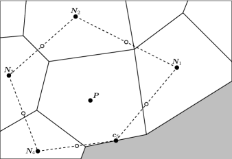
Figure 6: The divergence theorem method can approximate $\nabla\phi(\bm{P})$ to first-order accuracy on arbitrarily irregular grids if applied to the auxiliary cell bounded by dashed lines, rather than on the actual cell $P$. This cell is formed by joining the centroids of the neighbouring cells and of the boundary faces of cell $P$ by straight line segments. The open circles denote the centroids of these segments.

4 Gradient calculation using least squares minimisation

The starting point of the “least-squares” (LS) method for calculating the gradient of a quantity $\phi$ at the centroid of a cell $P$ is the expression of the values of $\phi$ at the centroids of all neighbouring cells as Taylor series expansions about the centroid of $P$. For convenience, we decompose the position vectors in Cartesian coordinates as $\bm{P}=(x_{0},y_{0})$, $\bm{N}_{f}=(x_{f},y_{f})$ and denote $\Delta x_{f}\equiv x_{f}-x_{0}$, $\Delta y_{f}\equiv y_{f}-y_{0}$. Then, for each neighbour $f$ it follows from the Taylor expansion that

$$\phi(\bm{N}_{f})-\phi(\bm{P})\;=\;\nabla\phi(\bm{P})\cdot(\bm{N}_{f}-\bm{P})\;+\;\varsigma_{f}$$ (24)

where

$$\varsigma_{f}\;=\;\frac{1}{2}\phi_{.xx}(\Delta x_{f})^{2}\;+\;\phi_{.xy}\,\Delta x_{f}\,\Delta y_{f}\;+\;\frac{1}{2}\phi_{.yy}(\Delta y_{f})^{2}\;+\;O(h^{3})$$ (25)

is an associated truncation error (the second derivatives are evaluated at $\bm{P}$). The basic idea of the method is to drop the unknown $\varsigma_{f}$ terms and solve the remaining linear system by least squares since, in general, the number of equations ($F$ = number of neighbouring cells) will be greater than the number of unknowns (two, $\phi_{\!.x}(\bm{P})$ and $\phi_{\!.y}(\bm{P})$). Of course some of the “neighbours” may be boundary face points such as the centroid $\bm{c}_{5}$ in Fig. 1, or, in the case of Neumann boundary conditions, the projection point $\bm{c}^{\prime}_{5}$. In the latter case $\phi(\bm{c}^{\prime}_{5})$ can be approximated by Eq. (23). Furthermore, unlike for the DT method, it is now easy to incorporate additional, more distant cells as neighbours, a practice that may prove advantageous in some cases (see e.g. [26]), although in the present work we will restrict ourselves to using only the cells that share a face with $P$.

It is advantageous to first multiply each equation $f$ by a suitably selected weight $w_{f}$ (weighted least squares). Then the system of all these equations can be written in matrix form as

$$\underbrace{\begin{bmatrix}w_{1}&\lx@intercol\hfil\text{\kern 10.00002pt\smash{\raisebox{-10.76385pt}{\Huge 0}}}\hfil\lx@intercol\\ &w_{2}&&\\ &&\ddots&\\ \lx@intercol\hfil\text{\kern-10.00002pt\smash{\raisebox{0.0pt}{\Huge 0}}}\hfil\lx@intercol&w_{F}\end{bmatrix}}_{W}\!\cdot\!\underbrace{\begin{bmatrix}\Delta\phi_{1}\\ \Delta\phi_{2}\\ \vdots\\ \Delta\phi_{F}\end{bmatrix}}_{b}\;=\;\underbrace{\begin{bmatrix}w_{1}&\lx@intercol\hfil\text{\kern 10.00002pt\smash{\raisebox{-10.76385pt}{\Huge 0}}}\hfil\lx@intercol\\ &w_{2}&&\\ &&\ddots&\\ \lx@intercol\hfil\text{\kern-10.00002pt\smash{\raisebox{0.0pt}{\Huge 0}}}\hfil\lx@intercol&w_{F}\end{bmatrix}}_{W}\!\cdot\!\left(\smash{\underbrace{\begin{bmatrix}\Delta x_{1}&\Delta y_{1}\\ \Delta x_{2}&\Delta y_{2}\\ \vdots&\vdots\\ \Delta x_{F}&\Delta y_{F}\end{bmatrix}}_{A}}\vphantom{\begin{bmatrix}\Delta x_{1}&\Delta y_{1}\\ \Delta x_{2}&\Delta y_{2}\\ \vdots&\vdots\\ \Delta x_{F}&\Delta y_{F}\end{bmatrix}}\!\cdot\!\smash{\underbrace{\begin{bmatrix}\phi_{\!.x}(\bm{P})\\[4.26773pt] \phi_{\!.y}(\bm{P})\end{bmatrix}\vphantom{\begin{bmatrix}w_{1}&\lx@intercol\hfil\text{\kern 10.00002pt\smash{\raisebox{-10.76385pt}{\Huge 0}}}\hfil\lx@intercol\\ &w_{2}&&\\ &&\ddots&\\ \lx@intercol\hfil\text{\kern-10.00002pt\smash{\raisebox{0.0pt}{\Huge 0}}}\hfil\lx@intercol&w_{F}\end{bmatrix}}}_{z}}\;+\;\smash{\underbrace{\begin{bmatrix}\varsigma_{1}\\ \varsigma_{2}\\ \vdots\\ \varsigma_{F}\end{bmatrix}}_{\varsigma}}\vphantom{\begin{bmatrix}\varsigma_{1}\\ \varsigma_{2}\\ \vdots\\ \varsigma_{F}\end{bmatrix}}\right)$$ (26)

where $\Delta\phi_{f}\equiv\phi(\bm{N}_{f})-\phi(\bm{P})$. The alternative matrix notation $Wb=W(Az+\varsigma)$ is also introduced above, to facilitate the discussions that follow. The above equations are exact, with the vector $\varsigma$ ensuring that the system (26) has a unique solution, which is independent of the weights, despite having more equations than unknowns. The redundant equations are just linear combinations of the non-redundant ones. But once $\varsigma$ is dropped, the system will, in general, have no solution.

Systems with no solution can be solved in the “least squares” sense [27, 28]. In matrix notation, if a linear system $Az=b$ with more equations than unknowns cannot be solved because the vector $b$ does not lie in the column space of the matrix $A$ then the best that can be done is to find the vector $z$ that minimises the error $b-Az$. This error will be minimised when its projection onto the column space of $A$ is zero, i.e. when $b-Az$ is perpendicular to each column of $A$, or $A^{\mathrm{T}}(b-Az)=0\Rightarrow A^{\mathrm{T}}Az=A^{\mathrm{T}}b$ (where $\mathrm{T}$ denotes the transpose). This latter system (called the normal equations) has a unique solution provided that $A$ has independent columns. The solution $z$ is called the least squares solution because it minimises the $L_{2}$ norm $\|b-Az\|$, i.e. the sum of the squares of the individual components of the error $e\equiv b-Az$ (note that each individual error component $e_{i}$ is the error of the corresponding equation $i$, $e_{i}=b_{i}-\sum_{j}a_{ij}z_{j}$).

In the weighted case $WAz=Wb$ the matrix $A$ is replaced by the product $WA$ and $b$ by $Wb$, so that the corresponding solution to the normal equations is

$$z\;=\;(A^{T}W^{\mathrm{T}}WA)^{-1}A^{\mathrm{T}}W^{\mathrm{T}}Wb$$ (27)

Now the quantity minimised is the norm of the error of the weighted system, $W(b-Az)=We$. Thus, if equation $i$ is assigned a larger weight than equation $j$ then the method will prefer to make $e_{i}$ small at the expense of $e_{j}$.

For now, we proceed with the least squares methodology on Eq. (26) without discarding $\varsigma$ in order to assess its impact on the error. We therefore first left-multiply the system (26) by $(WA)^{\mathrm{T}}$, and then solve it to obtain

$$z\;=\;(A^{\mathrm{T}}W^{\mathrm{T}}WA)^{-1}A^{\mathrm{T}}W^{\mathrm{T}}Wb\;+\;(A^{\mathrm{T}}W^{\mathrm{T}}WA)^{-1}A^{\mathrm{T}}W^{\mathrm{T}}W\varsigma$$ (28)

The matrix $A^{\mathrm{T}}W^{\mathrm{T}}WA$ is invertible provided that $WA$ has independent columns, which requires that $A$ have independent columns because $W$ is diagonal. The two columns of $A$ will be independent if there are also two independent rows, i.e. vectors $\bm{N}_{f}-\bm{P}$, so we need at least two neighbours $\bm{N}_{f}$ to lie at different directions with respect to $\bm{P}$, which is normally the case (in three dimensions $A$ has three columns and three independent neighbour directions are needed). Then, substituting for $A$, $W$, $z$, $b$ and $\varsigma$ from Eq. (26) into Eq. (28) and performing the matrix multiplications and inversions, we arrive at

$$z\;\equiv\;\nabla\phi(\bm{P})\;=\;\nabla^{\mathrm{ls}}\phi(\bm{P})\;+\;\tau$$ (29)

where $\nabla^{\mathrm{ls}}\phi(\bm{P})$ is the first term on the right side of Eq. (28),

$$\nabla^{\mathrm{ls}}\phi(\bm{P})\;\equiv\;\frac{1}{\mathrm{D}}\underbrace{\begin{bmatrix}\sum\limits_{f=1}^{F}(\Delta y_{f})^{2}w_{f}^{2}&-\sum\limits_{f=1}^{F}\Delta x_{f}\Delta y_{f}w_{f}^{2}\\[11.38092pt] -\sum\limits_{f=1}^{F}\Delta x_{f}\Delta y_{f}w_{f}^{2}&\sum\limits_{f=1}^{F}(\Delta x_{f})^{2}w_{f}^{2}\end{bmatrix}}_{M}\cdot\underbrace{\begin{bmatrix}\sum\limits_{f=1}^{F}\Delta x_{f}\Delta\phi_{f}w_{f}^{2}\\[11.38092pt] \sum\limits_{f=1}^{F}\Delta y_{f}\Delta\phi_{f}w_{f}^{2}\end{bmatrix}}_{\beta_{b}}$$ (30)

with $(1/D)M=(A^{\mathrm{T}}W^{\mathrm{T}}WA)^{-1}$ and $\beta_{b}=A^{\mathrm{T}}W^{\mathrm{T}}Wb$, and $\tau$ is the second term:

$$\tau\;=\;\frac{1}{\mathrm{D}}M\cdot\begin{bmatrix}\sum\limits_{f=1}^{F}\Delta x_{f}\varsigma_{f}w_{f}^{2}\;&\;\sum\limits_{f=1}^{F}\Delta y_{f}\varsigma_{f}w_{f}^{2}\end{bmatrix}^{\mathrm{T}}\;=\;\frac{1}{D}M\,\beta_{\varsigma}$$ (31)

with $\beta_{\varsigma}=A^{\mathrm{T}}W^{\mathrm{T}}W\varsigma$. In the 2D case, $D=|M|$, the determinant of $M$. Equation (29) gives the exact gradient $\nabla\phi(\bm{P})$, but since the truncation error $\tau$ is unknown we drop it and use the expression (30) alone as the approximate “least squares” gradient. In the 3D case the explicit formula is more involved than Eq. (30), but again the least squares gradient is obtained by solving Eq. (27). If, just for the purposes of discussing the 3D case, we denote the Cartesian components of the displacement vectors as $\bm{N}_{f}-\bm{P}=(\Delta x_{f}^{1},\Delta x_{f}^{2},\Delta x_{f}^{3})$, then the $(i,j)$ entry of the matrix $A^{\mathrm{T}}W^{\mathrm{T}}WA$ is $\sum_{f}\Delta x_{f}^{i}\Delta x_{f}^{j}w_{f}^{2}$ (it is a symmetric matrix) and the $i$-th component of the vector $A^{\mathrm{T}}W^{\mathrm{T}}Wb$ is $\sum_{f}\Delta x_{f}^{i}\Delta\phi_{f}w_{f}^{2}$. The normal equations (27) are sometimes ill-conditioned, and in such cases it is better to solve the least-squares system by $QR$ factorisation of $A$ [27].

The above derivation has produced the explicit expression (31) for the truncation error $\tau$. To analyse it further, we can assume that all the weights share the same dependency on the grid spacing, namely $w_{f}=O(h^{q})$ for some real number $q$ (independent of $f$), as is the usual practice. Then the factors of Eq. (31) have the following magnitudes: Since $\Delta x_{f}$ and $\Delta y_{f}$ are $O(h)$ the coefficients of $M$ have magnitude $O(h^{2+2q})$. Consequently, $M$ being $2\times 2$, its determinant will have magnitude $(O(h^{2+2q}))^{2}\Rightarrow 1/D=O(h^{-2(2+2q)})$. Finally, considering that $\varsigma_{f}=O(h^{2})$, the components of $\beta_{\varsigma}$ are of $O(h^{2q+3})$. Multiplying all these together, Eq. (31) shows that $\tau=O(h)$, independently of $q$. This is not surprising, given that the approximation is based on Eq. (24) which assumes a linear variation of $\phi$ in the vicinity of point $\bm{P}$. So, $\nabla^{\mathrm{ls}}$ is at least first order accurate, even on grids of arbitrary geometry.

The order of accuracy of $\nabla^{\mathrm{ls}}$ may be higher than one if some cancellation occurs between the components of $\tau$ for certain grid configurations, similarly to the DT operator. In particular, a tedious but straightforward calculation shows that when applied to a parallelogram grid such as that shown in Fig. 2, $\nabla^{\mathrm{ls}}$ again reduces to the second-order accurate formula (1), provided only that the weights of parallel faces are equal: $w_{1}=w_{3}$ and $w_{2}=w_{4}$. This will hold due to symmetry if the weights are dependent only on the grid geometry. Of course, as for the DT gradient, this has the consequence that the LS gradient is second-order accurate also on smooth curvilinear structured grids.

The choice of weights

According to the preceding analysis, the least squares method is first-order accurate on grids of arbitrary geometry and second-order accurate on smooth structured grids. This holds irrespective of the choice of weights, and in fact it holds even for the unweighted method ($w_{f}=1$). The question then arises of whether a suitable choice of weights can offer some advantage.

The weights commonly used are of the form $w_{f}=(\Delta r_{f})^{-q}$ where $\Delta r_{f}=\|\bm{N}_{f}-\bm{P}\|$ is the distance between the two cell centres and $q$ is an integer, usually chosen as $q=1$ [12, 16, 11] or $q=2$ [14, 6]. The unweighted method amounts to $q=0$. As noted, the least squares method finds the approximate gradient that minimises $\|W(b-Az)\|$, which for the various choices of $q$ amounts to minimising:

$$q=0:\qquad \sum_{f}\left[\Delta r_{f}\left(\frac{\Delta\phi_{f}}{\Delta r_{f}}\;-\;\nabla^{\mathrm{ls}}\phi(\bm{P})\cdot\bm{d}_{f}\right)\right]^{2}$$ (32)

$$q=1:\qquad \sum_{f}\left(\frac{\Delta\phi_{f}}{\Delta r_{f}}\;-\;\nabla^{\mathrm{ls}}\phi(\bm{P})\cdot\bm{d}_{f}\right)^{2}$$ (33)

$$q=2:\qquad \sum_{f}\left[\frac{1}{\Delta r_{f}}\left(\frac{\Delta\phi_{f}}{\Delta r_{f}}\;-\;\nabla^{\mathrm{ls}}\phi(\bm{P})\cdot\bm{d}_{f}\right)\right]^{2}$$ (34)

where $\bm{d}_{f}=(\bm{N}_{f}-\bm{P})/\Delta r_{f}$ is the unit vector in the direction from $\bm{P}$ to $\bm{N}_{f}$, and so $\nabla^{\mathrm{ls}}\phi\cdot\bm{d}_{f}$ is the least squares directional derivative $\partial\phi/\partial r_{f}$ in that direction. In the $q=1$ case, expression (33) shows that the least squares procedure shows no preference in trying to set the directional derivative in each neighbour direction $f$ equal to the finite difference $\Delta\phi_{f}/\Delta r_{f}$. On the other hand, in the unweighted method (32) the discrepancies between the directional derivatives and the finite differences are weighted by the distances $\Delta r_{f}$ so that the method prefers to reduce $\Delta\phi/\Delta r_{f}-\nabla^{\mathrm{ls}}\phi\cdot\bm{d}_{f}$ along the directions of the distant neighbours at the expense of the directions of the closer neighbours. The exact opposite holds for the $q=2$ case (34) where the discrepancies are weighted by $1/\Delta r_{f}$ so that the result is determined mostly by the close neighbours. Intuitively, this latter choice seems more reasonable as the linearity of the variation of $\phi$ is lost as one moves away from $\bm{P}$ and thus at distant neighbours the finite differences $\Delta\phi/\Delta r_{f}$ are less accurate approximations of the directional derivatives. Thus it is not surprising that usually the $q>0$ methods outperform the unweighted method.

These are the common weight choices, but it so happens that the particular non-integer exponent $q=3/2$ confers enhanced accuracy compared to the other $q$ choices under special but not uncommon circumstances. This fact does not appear to be widely known in the literature; we have seen it only briefly mentioned in [29, 18]. So, consider the vector $\beta_{\varsigma}$ in the expression (31) for the error, and substitute for $\varsigma$ from Eq. (25). Then the first component of $\beta_{\tau}$ becomes

$$\sum_{f}\Delta x_{f}\,\varsigma_{f}\,w_{f}^{2}\; =\;\frac{\phi_{.xx}}{2}\sum_{f}(\Delta x_{f})^{3}w_{f}^{2}\;+\;\phi_{.xy}\sum_{f}(\Delta x_{f})^{2}\Delta y_{f}\,w_{f}^{2}\;+\;\frac{\phi_{.yy}}{2}\sum_{f}\Delta x_{f}\,(\Delta y_{f})^{2}w_{f}^{2}$$

$$+\;\sum_{f}O(h^{4})\,w_{f}^{2}$$ (35)

Now, if two neighbours, $i$ and $j$ say, lie at opposite directions to point $\bm{P}$ but at the same distance then $w_{i}=w_{j}$, $\Delta x_{i}=-\Delta x_{j}$ and $\Delta y_{i}=-\Delta y_{j}$ so that their contributions in each of the first three sums in the right hand side of Eq. (35) cancel out. If all neighbour points are arranged in such pairs, like in the grid of Fig. 2, then these three sums become zero leaving only the $\sum O(h^{4})w_{f}^{2}$ term. The same holds for the second component of $\beta_{\varsigma}$, so that $\beta_{\varsigma}=O(h^{4-2q})$ overall because $w_{f}=O(h^{-q})$. Then Eq. (31) gives $\tau=(1/D)M\beta_{\varsigma}=O(h^{2})$ i.e. the method is second-order accurate for any exponent $q$.

The particular choice $w_{f}=(\Delta r_{f})^{-3/2}$ amounts to dropping the $w_{f}$’s from the first three sums of the right-hand side of Eq. (35) and replacing therein every instance of $\Delta x_{f}$ by $\Delta x_{f}/\Delta r_{f}$ and every instance of $\Delta y_{f}$ by $\Delta y_{f}/\Delta r_{f}$. These ratios are precisely $\cos\theta_{f}$ and $\sin\theta_{f}$, respectively, where $\theta_{f}$ is the angle that the direction vector $\bm{N}_{f}-\bm{P}$ makes with the horizontal direction. If two neighbours, $i$ and $j$, lie at opposite directions then $\theta_{i}=\theta_{j}+\pi$ so that $\cos\theta_{i}=-\cos\theta_{j}$ and $\sin\theta_{i}=-\sin\theta_{j}$, and their contributions cancel out in the aforementioned three sums, irrespective of whether these two neighbours lie at equal distances to $\bm{P}$ or not. The same holds for the second component of $\beta_{\varsigma}$. Thus, if all neighbour points are arranged in such pairs then again what remains of the right-hand side of Eq. (35) is only the last term and so $\tau=O(h^{2})$. For example, the LS gradient with $q=3/2$ is second-order accurate at the boundary volume $P$ of Fig. 4, whereas it is only first-order accurate with any other choice of $q$. Furthermore, the same result will hold if the neighbours are not arranged in pairs at opposite directions but tend to become so with grid refinement. This is the case with smooth structured grids, as shown in Section 2, and therefore the LS gradient with $q=3/2$ is second-order accurate at boundary cells of all smooth structured grids.

Another property of the $q=3/2$ LS gradient is that it is second order accurate if all neighbour points are arranged at equal angles. Unfortunately, this property holds only with more than three neighbour points, which limits its usefulness. A proof is provided in Appendix A.

Finally, a question that arises naturally is whether full 2nd-order accuracy can be achieved on arbitrary grids by allowing non-diagonal entries in the weights matrix. It turns out that this is indeed possible, but yields a method that is equivalent to the least squares solution of a system of Taylor expansions (24) with terms higher than first-order included. The procedure is sketched in Appendix B. We do not advocate it, because direct solution of the system of higher-order Taylor expansions would have the added advantage of solving also for the second derivatives – see e.g. [30]. An alternative second-order accurate method is described in [31]. The second-order accurate methods are much more expensive than the present method.

5 Numerical tests on the accuracy of the gradient schemes

5.1 One-dimensional tests

The methods are first tested on a one-dimensional problem so as to examine the effect of unevenness, isolated from skewness. The derivative of the single-variable function $\phi(x)=\tanh x$ is calculated at 101 equispaced points spanning the $x\in[0,2]$ interval. The results are compared against the exact solution $\phi_{\!.x}=1-(\tanh x)^{2}$ and the mean absolute error $\sum_{i}|\phi_{\!.x}(x_{(i)})-\phi_{\!.x}^{\mathrm{ls}}(x_{(i)})|/101$ is recorded for each method. In order to introduce unevenness, the neighbours of point $x_{i}$ are not chosen from this set of equispaced points but are set at $x_{i,f}=x_{i}+\Delta x_{f}/2^{r}$ where the $\Delta x_{f}$ belong to a predetermined set of displacements $\{\Delta x_{f}\}_{f=1}^{F}$ (common to all $x_{i}$ points) and the integer $r$ is the level of grid refinement. For example, if the chosen set of displacements is $\{-0.05,0.1\}$ ($F$ = 2 neighbours), then the derivative at point $x_{i}$ will be calculated using the values of $\phi$ at the three points $\{x_{i}-0.05/2^{r},\;x_{i},\;x_{i}+0.1/2^{r}\}$. The order of accuracy of each method is determined by incrementing the level of refinement $r$.

In order to test the methods thoroughly, several sets of initial displacements $\{\Delta x_{f}^{0}\}_{f=1}^{F}$ were used. In Fig.  7, each diagram corresponds to a different such set and the mean error is plotted as a function of the number of displacement halvings, $r$. The slope of each curve reveals the order of accuracy of the corresponding method. The methods tested are: (a) the DT method, denoted “d”, (b) the LS methods with weight exponents $q=0,1,1.5,2$ and $3$, indicated on each curve, (c) the non-diagonal weights LS method of Appendix B denoted “ND”, and (d) a simpler variant of the DT method which is sometimes used [20], denoted “da”, where the values at face centres are calculated by arithmetic averaging, $\phi(\bm{c}^{\prime}_{f})=(\phi(\bm{P})+\phi(\bm{N}))/2$, instead of linear interpolation (9). The DT methods are only applicable in the case plotted in Fig. 7(b) because exactly two neighbours are required, one on each side of $x_{i}$. To apply the DT methods $x_{i}$ is regarded as the centroid of a cell of size equal to the minimum distance between $x_{i}$ and any of its neighbours.

(a) $\{\Delta x_{f}^{0}\}=\{0.05,0.10\}$

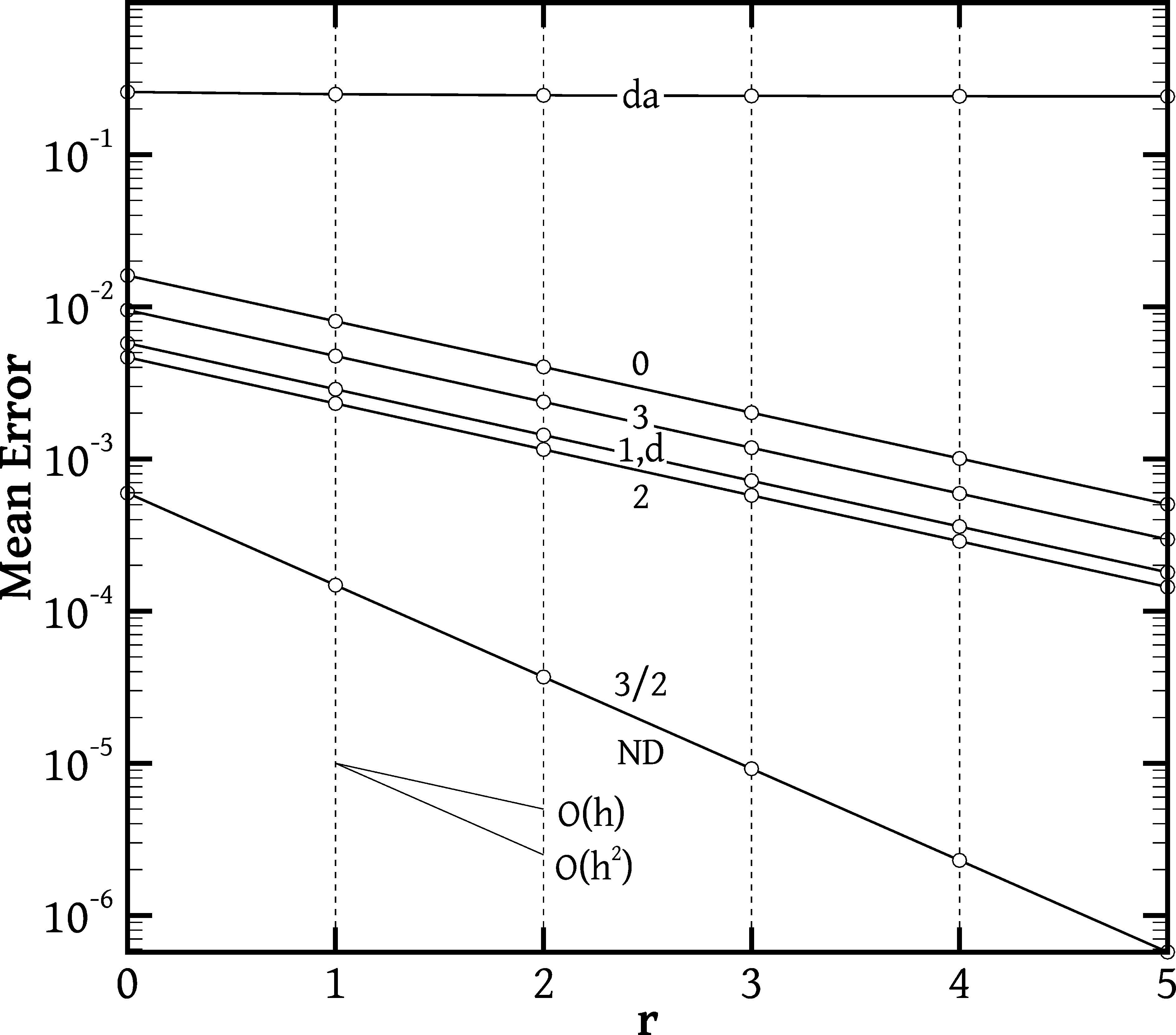
(b) $\{\Delta x_{f}^{0}\}=\{-0.10,0.05\}$

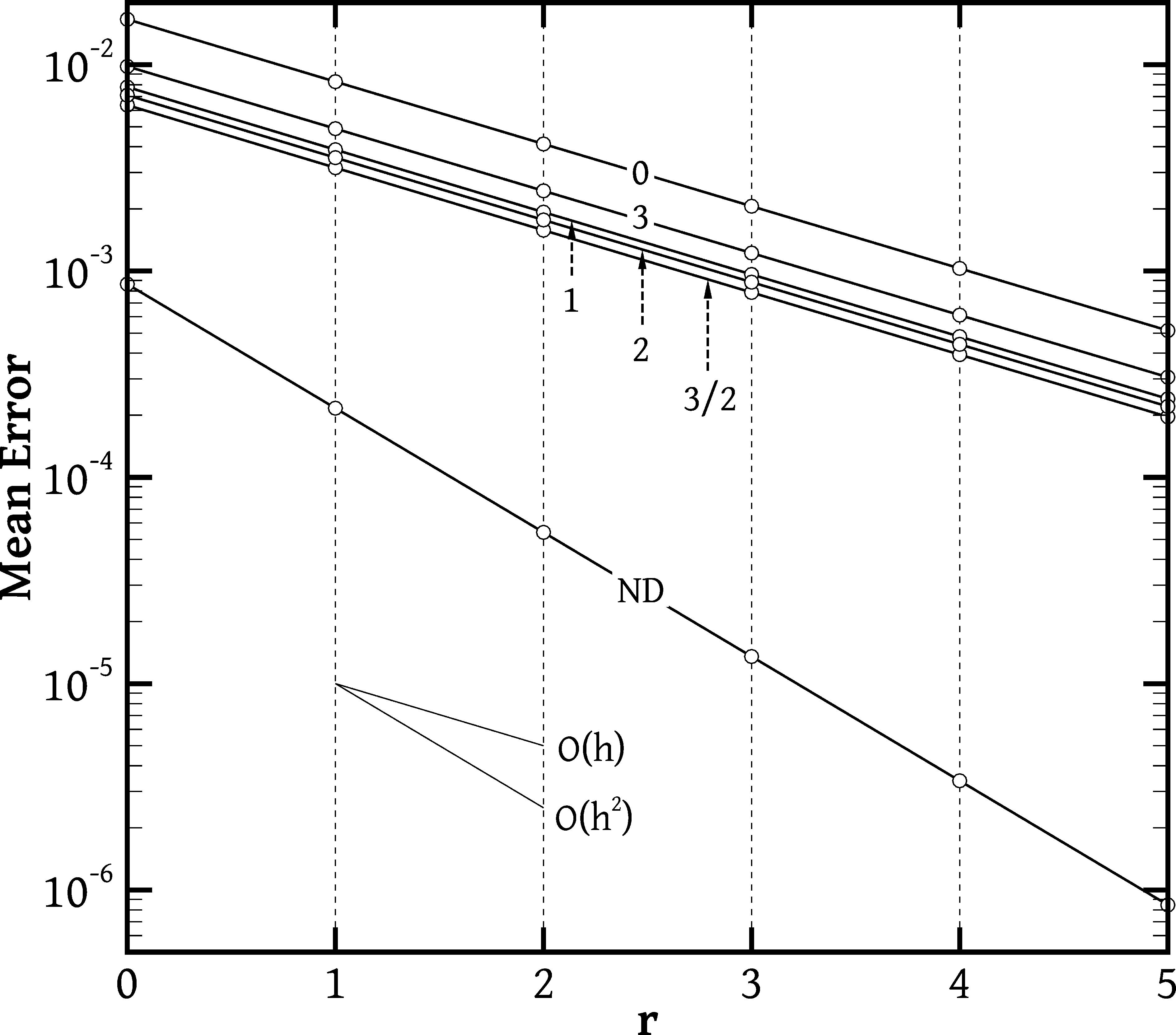
(c) $\{\Delta x_{f}^{0}\}=\{-0.10,0.05,0.15\}$

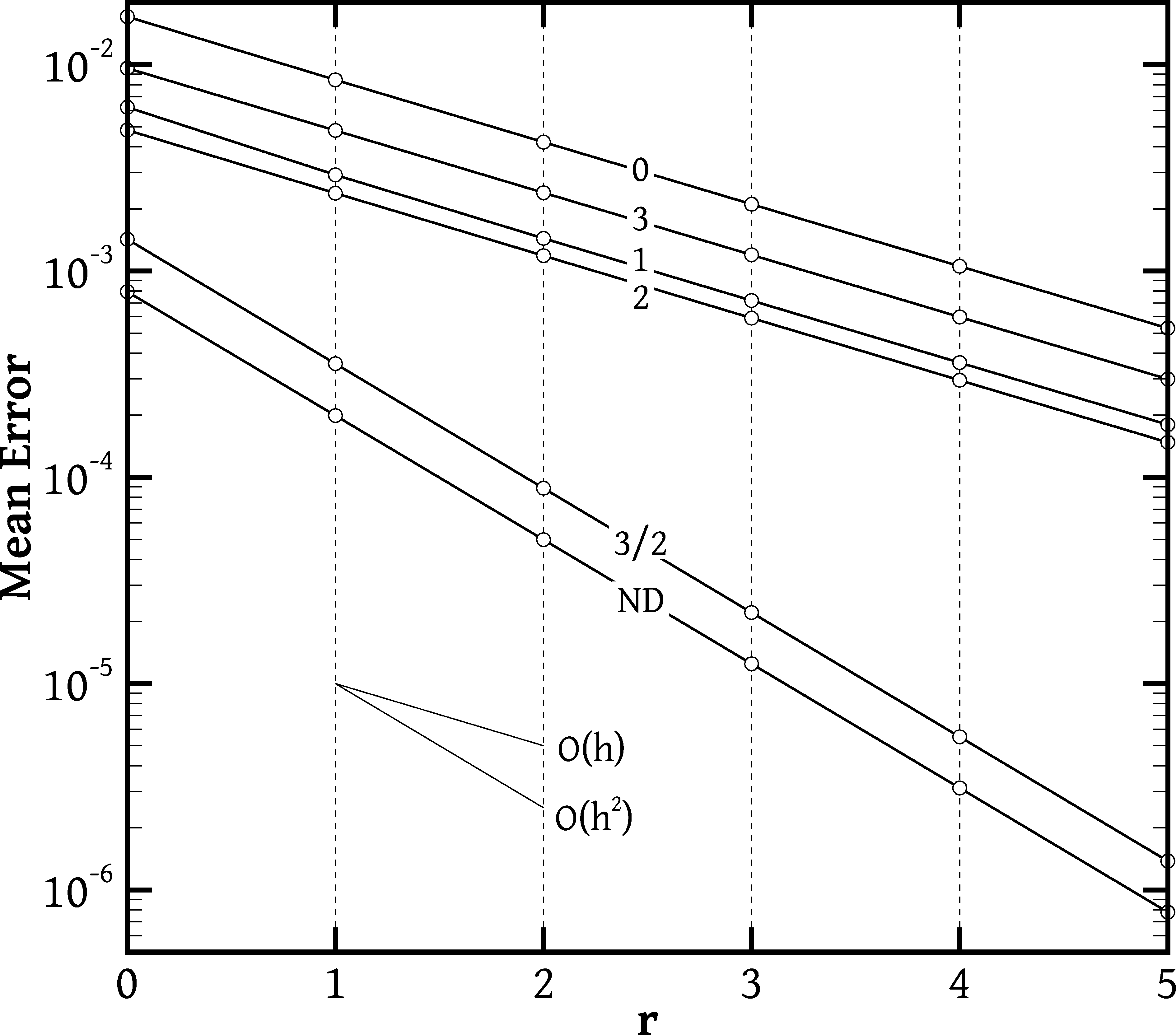
(d) $\{\Delta x_{f}^{0}\}=\{-0.20,-0.10,0.05,0.15\}$

Figure 7: Mean errors of the calculation of the derivative of $\phi(x)=\tanh(x)$ with various methods – see the text for details.

A result not shown is that when the displacements stencil is symmetric (e.g. $\{\Delta x_{f}^{0}\}=\{-0.1,0.1\}$) all methods produce identical, second-order accurate results. This is consistent with the two-dimensional case where on symmetric grids like that of Fig. 2 all methods reduce to the formula (1). When the stencil is not symmetric, Fig. 7 shows that the LS methods with a diagonal weights matrix become first-order accurate, except for the $q=3/2$ method which retains second-order accuracy when there are equal numbers of neighbours on either side (Figs. 7(b) and 7(d)). The unweighted method ($q=0$) is always the least accurate; the optimum accuracy is achieved with $1\leq q\leq 2$, while a further increase of $q$ is unprofitable ($q=3$). The method of Appendix B is always second-order accurate. Concerning the DT methods (Fig. 7(b)), the method of Sec. 3, indicated by “d” in the figure, gives identical results with the $q=1$ least squares method. On the other hand, the simplified method, indicated by “da”, is zeroth-order accurate, which agrees with the findings reported in [20].

5.2 Uniform Cartesian grids

Next, the two-dimensional methods are used to calculate the gradient of the function $\phi(x,y)=\tanh(x)\!\cdot\!\tanh(y)$ on the unit square $(x,y)\in[0,1]\times[0,1]$ using uniform Cartesian grids of different fineness. The exact gradient is $\phi_{\!.x}=(1-(\tanh x)^{2})\tanh y$ and $\phi_{\!.y}=(1-(\tanh y)^{2})\tanh x$. All grid cells are geometrically identical squares of side $h=0.25/2^{r}$ where $r$ is the level of refinement; however, boundary cells are topologically different from interior cells because they have one or more boundary faces where the function value at the face centre has to be used (Fig. 4). It so happens that the function $\tanh$ has zero second derivative at the boundaries $x=0$ and $y=0$, which may artificially increase the order of accuracy of the methods there. However, the general behaviour of the methods at boundary cells can be observed at the $x=1$ and $y=1$ boundaries where no such special behaviour of the $\tanh$ function applies.

On each grid the gradient of $\phi$ is calculated at all cell centres using the DT method $\nabla^{\mathrm{d}0}$ (Eq. (10)), and the LS methods $\nabla^{\mathrm{ls}}$ (Eq. (30)) with weight exponents $q=0,1,1.5$ and $2$. Since there is no skewness ($\bm{c}^{\prime}=\bm{c}$ in Eq. (16)), the application of corrector steps is meaningless. The methods are evaluated by comparing the mean and maximum truncation errors, defined as

$$\tau_{\mathrm{mean}}\; \equiv\;\frac{1}{M_{r}}\sum_{P=1}^{M_{r}}\|\nabla^{\mathrm{a}}\phi(\bm{P})-\nabla\phi(\bm{P})\|$$ (36)

$$\tau_{\mathrm{max}}\; \equiv\;\max_{P=1}^{M_{r}}\|\nabla^{\mathrm{a}}\phi(\bm{P})-\nabla\phi(\bm{P})\|$$ (37)

where $\|\cdot\|$ denotes the $L_{2}$ norm of a vector in a single cell, $M_{r}$ is the number of cells of grid $r$, and $\nabla^{\mathrm{a}}$ is any of the gradient schemes considered. These errors are plotted in Figs. 8(a) and 8(b), respectively.

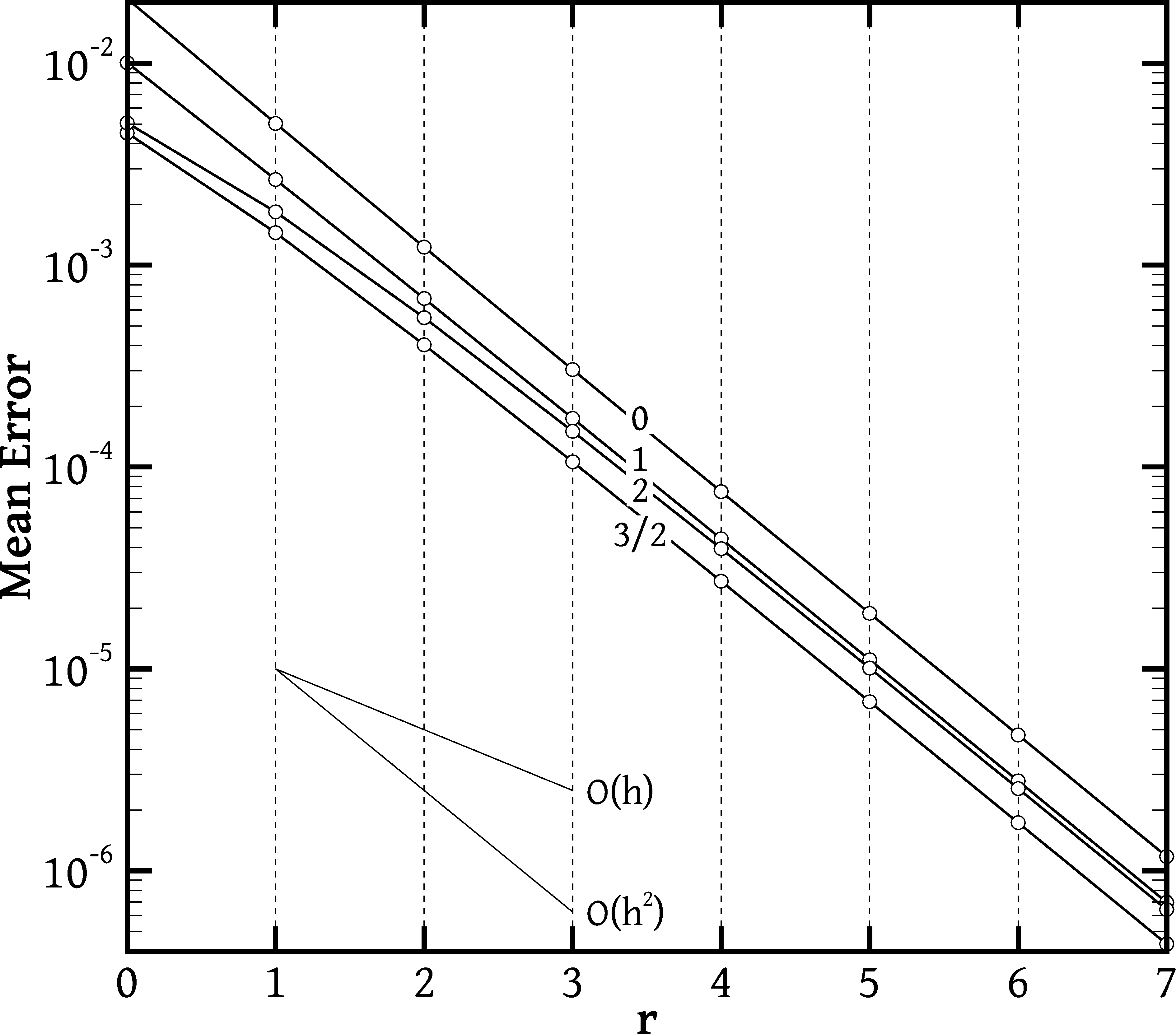
(a) mean error, $\tau_{\mathrm{mean}}$

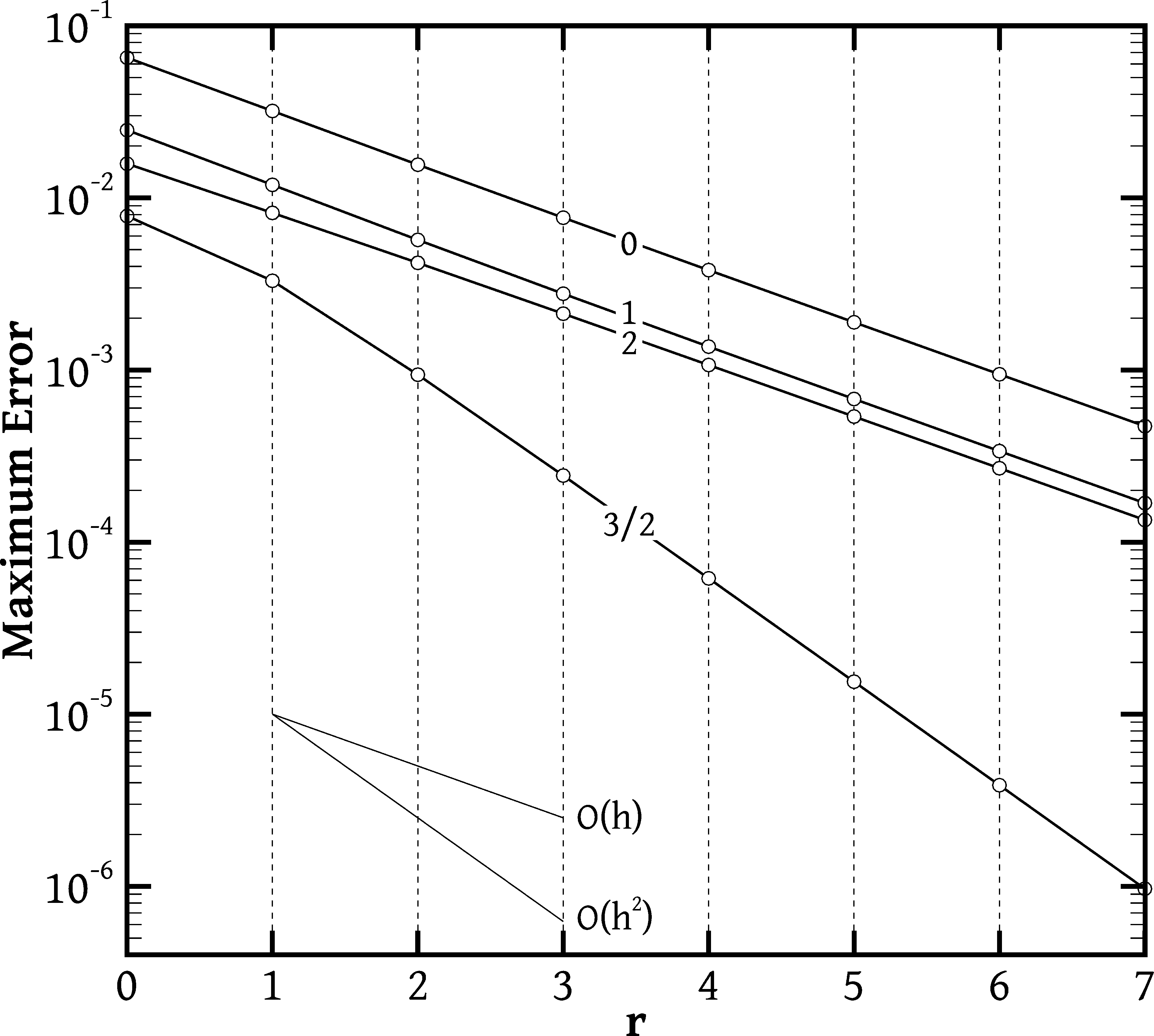
(b) maximum error, $\tau_{\mathrm{max}}$

Figure 8: The mean 8(a) and maximum 8(b) errors (defined by Eqs. (36) and (37), respectively) of the various methods for calculating the gradient of the function $\phi=\tanh(x)\tanh(y)$ on uniform Cartesian grids. The abscissa $r$ designates the grid; grid $r$ has a uniform spacing of $h=0.25/2^{r}$. The exponent $q$ used for the LS weights is shown on each curve. The DT method produces identical results with the $q$ = 1 LS method.

The theory predicts that all methods should be second-order accurate at interior cells, i.e. $\bm{\tau}=O(h^{2})$, because they all reduce to formula (1) there. At boundary cells (Fig. 4) the favourable conditions that are responsible for second-order accuracy are lost, and the methods should revert to first-order accuracy except for the LS method with $q=3/2$ of which second-order accuracy is still expected. Figure 8(b) confirms that the maximum error, which occurs at some boundary cell, is $\tau_{\mathrm{max}}=O(h)$ for all methods, except the $q=3/2$ method for which $\tau_{\mathrm{max}}=O(h^{2})$. Of the other methods, the unweighted LS method ($q=0$) is the least accurate and the $q=2$ method is slightly better than the $q=1$ method. The DT method gives identical results with the $q=1$ LS method, as they both revert to Eq. (13) at boundary cells.

Figure 8(a) shows the mean errors. Since all methods give the same results at interior cells any differences are due to the different errors at the boundary cells. The slope of the curves is the same, and corresponds to $\tau_{\mathrm{mean}}=O(h^{2})$. This does not contradict with the $O(h)$ errors at the boundary cells: the number of such cells along each side of the domain equals $1/h$, so that in total there are $O(1/h)$ boundary cells, each contributing an $O(h)$ error. Their total contribution to $\tau_{\mathrm{mean}}$ in Eq. (36) is therefore $O(1/h)\!\cdot\!O(h)/M_{r}=O(h^{2})$ since $M_{r}=1/h^{2}$. The interior cell contribution is $O(h^{2})$ also, since $\tau=O(h^{2})$ at each individual interior cell.

5.3 Smooth curvilinear grids

Next, we try the methods on smooth curvilinear grids. The same function $\phi=\tanh(x)\!\cdot\!\tanh(y)$ is differentiated, but the domain boundaries now have the shapes of two horizontal and two vertical sinusoidal waves (Fig. 9), beginning and ending at the points $(0,0)$, $(1,0)$, $(1,1)$ and $(0,1)$. The grid is generated using a very basic elliptic grid generation method [32]. In particular, smoothly varying functions $\xi(x,y)$ and $\eta(x,y)$ are assumed in the domain, and the grid consists of lines of constant $\xi$ and of constant $\eta$. The left, right, bottom and top boundaries correspond to $\xi=0$, $\xi=1$, $\eta=0$ and $\eta=1$, respectively. In the interior of the domain $\xi$ and $\eta$ are assumed to vary according to the following Laplace equations:

$$\xi_{.xx}\;+\;\xi_{.yy}\; =\;0$$

$$\eta_{.xx}\;+\;\eta_{.yy}\; =\;0$$

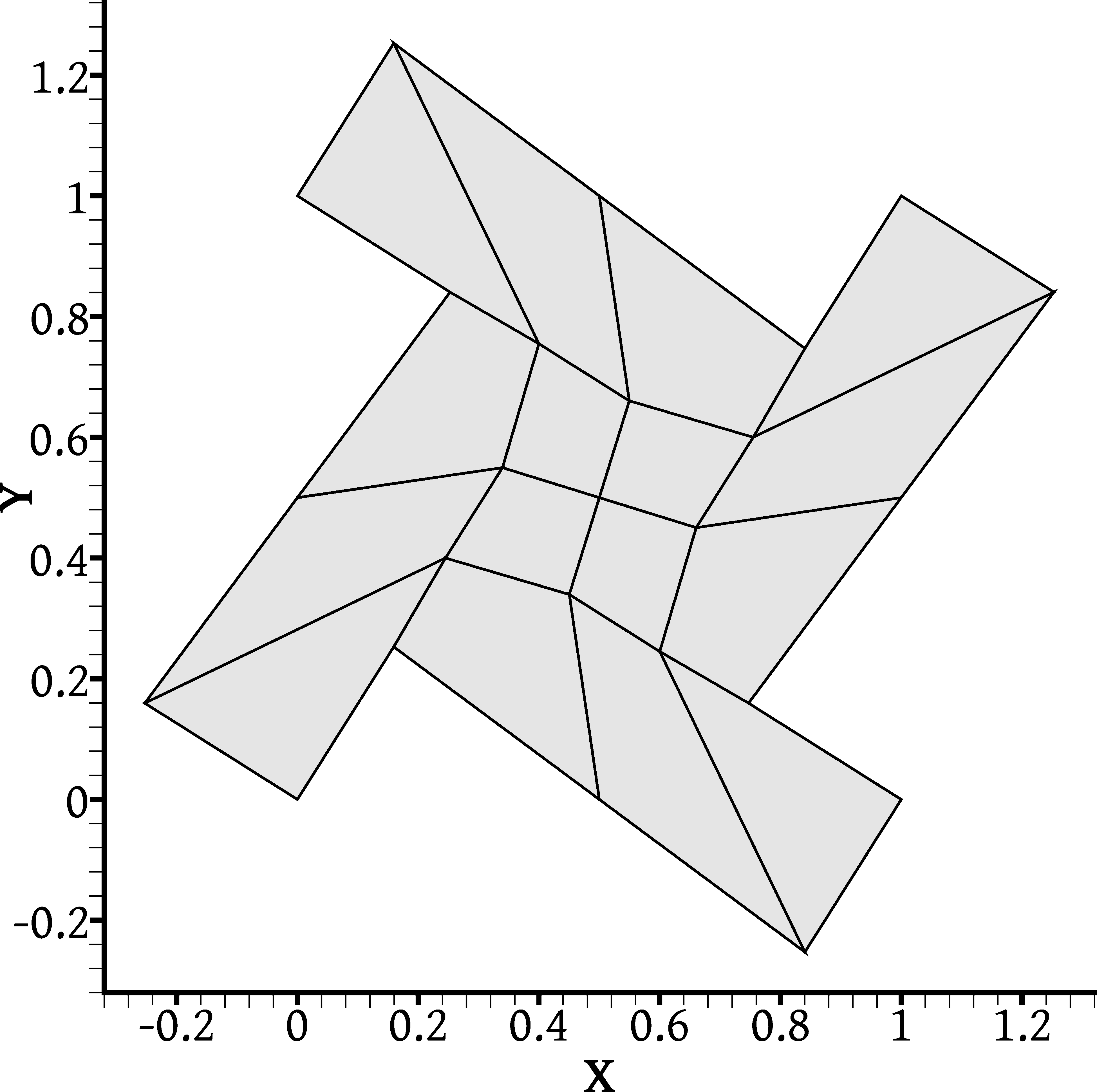
(a) $r=0$

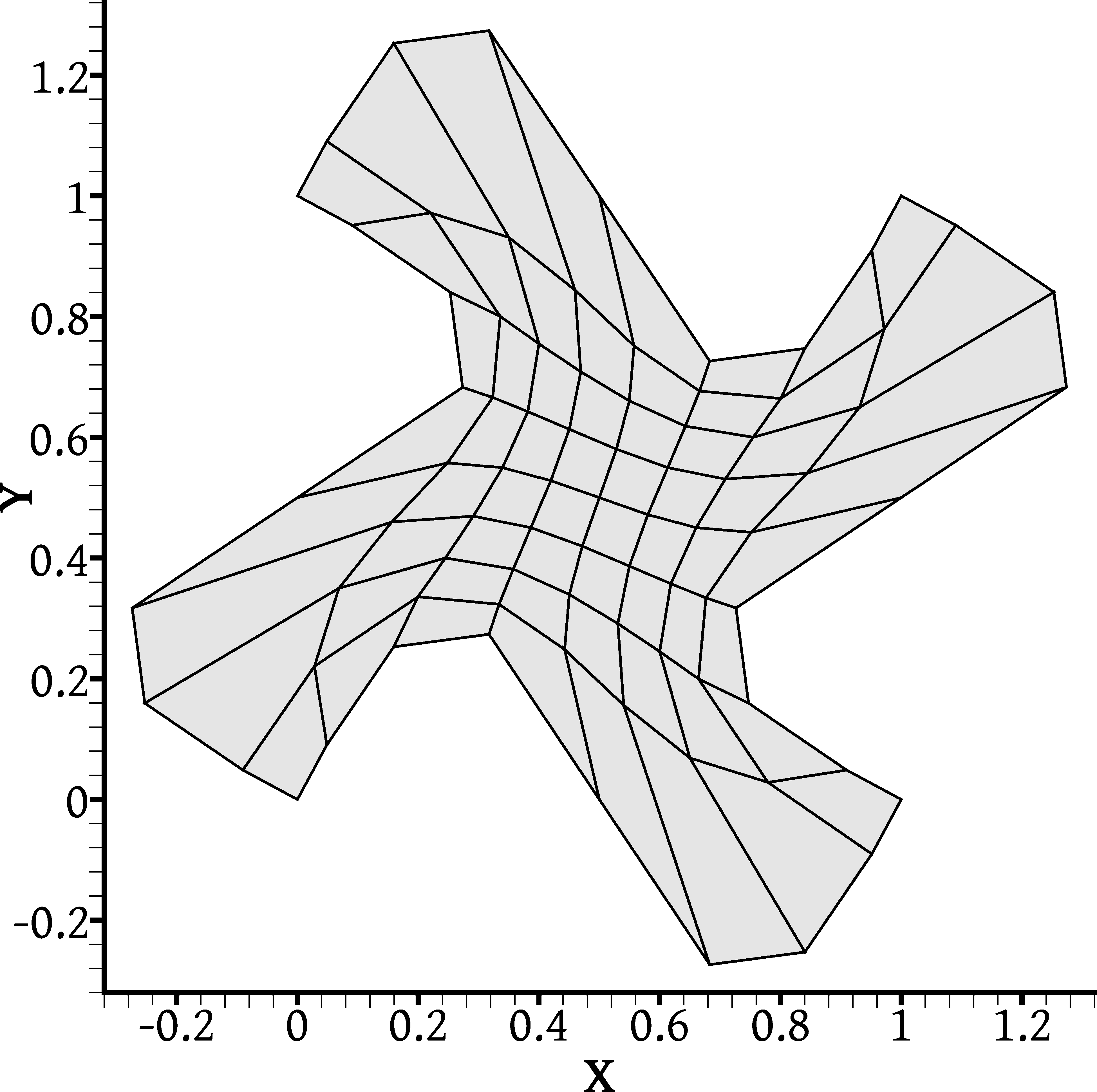
(b) $r=1$

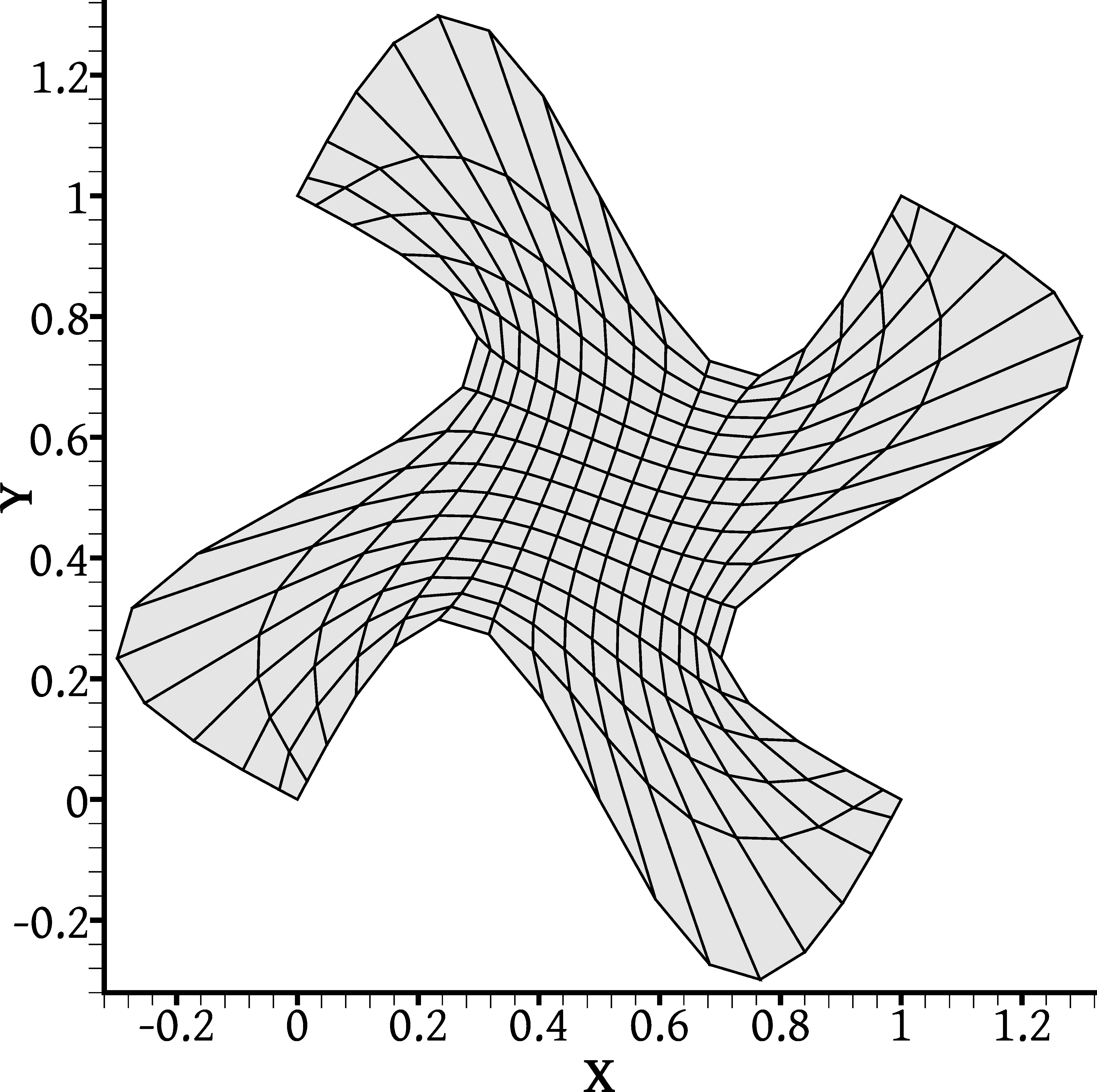
(c) $r=2$

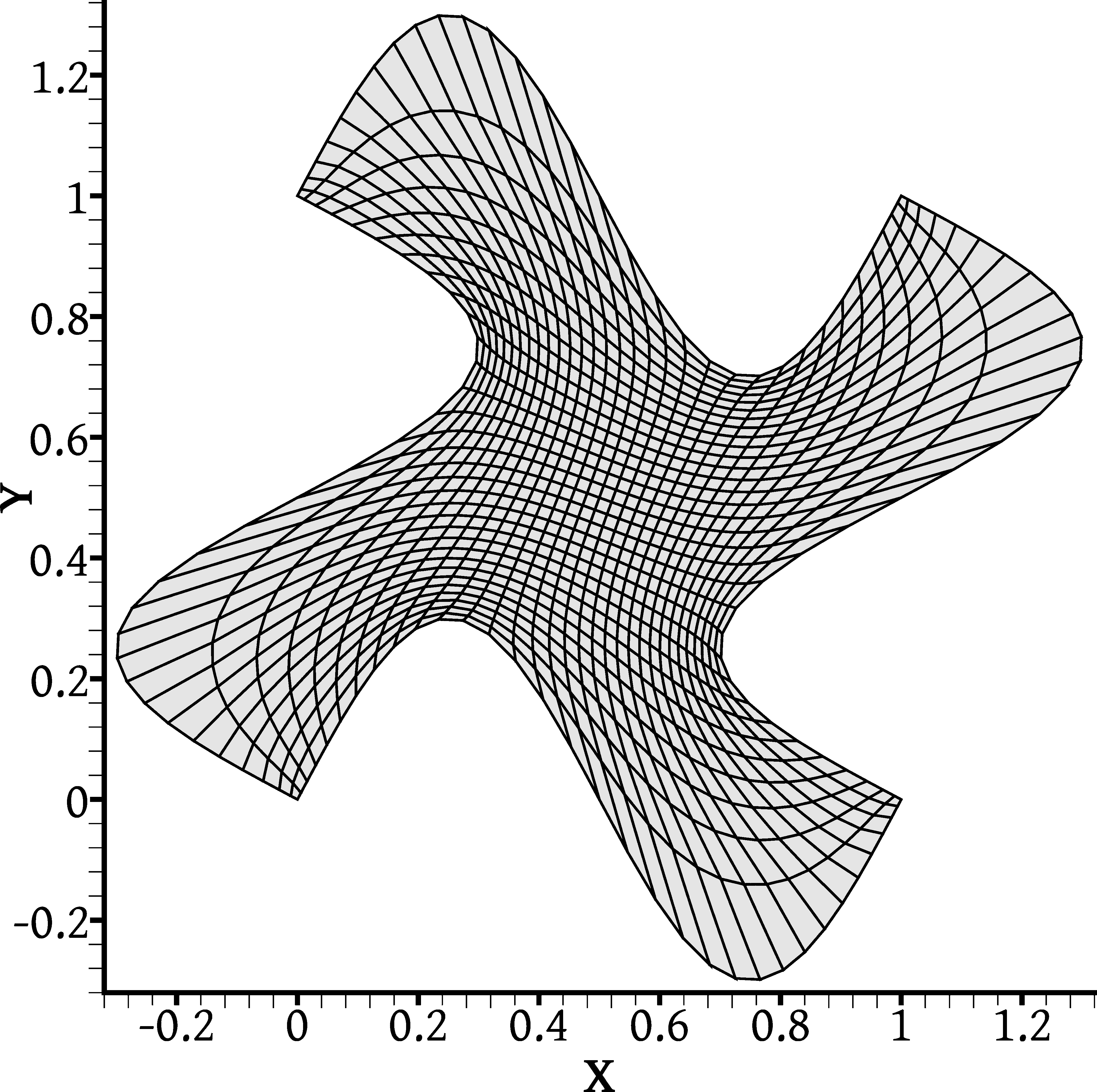
(d) $r=3$

Figure 9: The first four of the series of grids constructed on a domain with sinusoidal boundaries via elliptic grid generation. See the text for more details.

These equations guarantee that $\xi$ and $\eta$ vary smoothly in the domain, but their solution $\xi=\xi(x,y)$, $\eta=\eta(x,y)$ is not much help in constructing the grid. Instead, we need the inverse functions $x=x(\xi,\eta)$, $y=y(\xi,\eta)$ which explicitly set the locations of all grid nodes; node $(i,j)$ is located at $(x_{i,j},y_{i,j})\equiv(x(\xi=i\,\Delta\xi,\eta=j\,\Delta\eta),y(\xi=i\,\Delta\xi,\eta=j\,\Delta\eta))$. With $\xi,\eta\in[0,1]$, the constant spacings $\Delta\xi$ and $\Delta\eta$ are adjusted according to the desired grid fineness. Therefore, using the chain rule of partial differentiation it can be shown that the above equations can be expressed in inverse form as

$$g_{22}\,x_{\!.\xi\xi}\;-\;2g_{12}\,x_{\!.\xi\eta}\;+\;g_{11}\,x_{\!.\eta\eta}\; =\;0$$

$$g_{22}\,y_{\!.\xi\xi}\;-\;2g_{12}\,y_{\!.\xi\eta}\;+\;g_{11}\,y_{\!.\eta\eta}\; =\;0$$

where

$$g_{11}\; =\;x^{2}_{\!.\xi}+y^{2}_{\!.\xi}$$

$$g_{22}\; =\;x^{2}_{\!.\eta}+y^{2}_{\!.\eta}$$

$$g_{12}\; =\;x_{\!.\xi}x_{\!.\eta}+y_{\!.\xi}y_{\!.\eta}$$

In order to cluster the points near the boundaries in the physical domain, we accompany the above equations with the following boundary conditions: at the bottom boundary we set $x=0.5+0.5\sin(\pi(\xi-0.5))$ and $y=\sin(2\pi x)$, and at the left boundary we set $y=0.5+0.5\sin(\pi(\eta-0.5))$ and $x=-\sin(2\pi y)$. At the top and right boundaries we set the same conditions, respectively, adding 1 to $x$ at the right boundary and 1 to $y$ at the top boundary. Better results can be obtained by using a more elaborate method such as described in [33], but this suffices for the present purposes.

Now $(x,y)$ have become the dependent variables while $(\xi,\eta)$ are the independent variables, which acquire values in the unit square $[0,1]\times[0,1]$. The grid equations were solved numerically with a finite difference method on a $513\times 513$ point uniform Cartesian grid. Note that the dependent variables $(x,y)$ are stored at the grid nodes, i.e. at the intersection points of the grid lines, instead of at the cell centres. The derivatives are approximated by second-order accurate central differences; for example, at point $(i,j)$, $x_{\!.\xi}\approx(x_{i+1,j}-x_{i-1,j})/2h$, $x_{\!.\eta}\approx(x_{i,j+1}-x_{i,j-1})/2h$, $x_{\!.\xi\xi}\approx(x_{i+1,j}-2x_{i,j}+x_{i-1,j})/h^{2}$ etc. where $h=1/512$ is the grid spacing. The resulting system of nonlinear algebraic equations was solved using a Gauss-Seidel iterative method where in the equations of the $(i,j)$ node all terms are treated as known from their current values except for $x_{i,j}$ and $y_{i,j}$ which are solved for. The convergence of the method was accelerated using a minimal polynomial extrapolation technique [34], and iterations were carried out until machine precision was reached.

After obtaining $x(\xi,\eta)$ and $y(\xi,\eta)$, a series of successively refined grids in the physical domain were constructed by drawing lines of constant $\xi$ and lines of constant $\eta$ at intervals $\Delta\xi=\Delta\eta=0.25/2^{r}$, for $r=0,1,\ldots 7$. The first four grids are shown in Fig. 9. The gradient calculation methods were then applied on each of these grids. The errors of each method are depicted in Fig. 10.

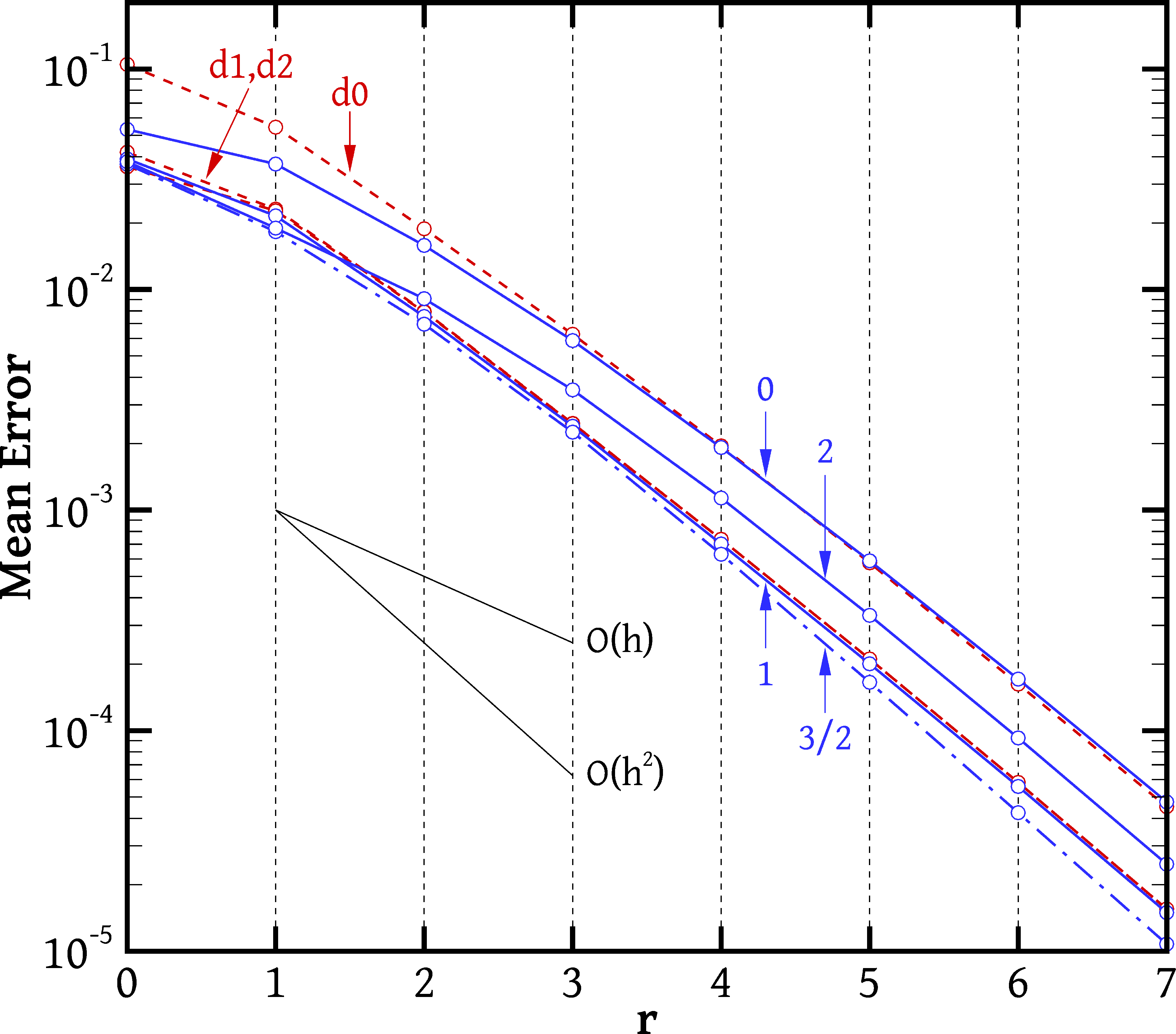
(a) mean error, $\tau_{\mathrm{mean}}$

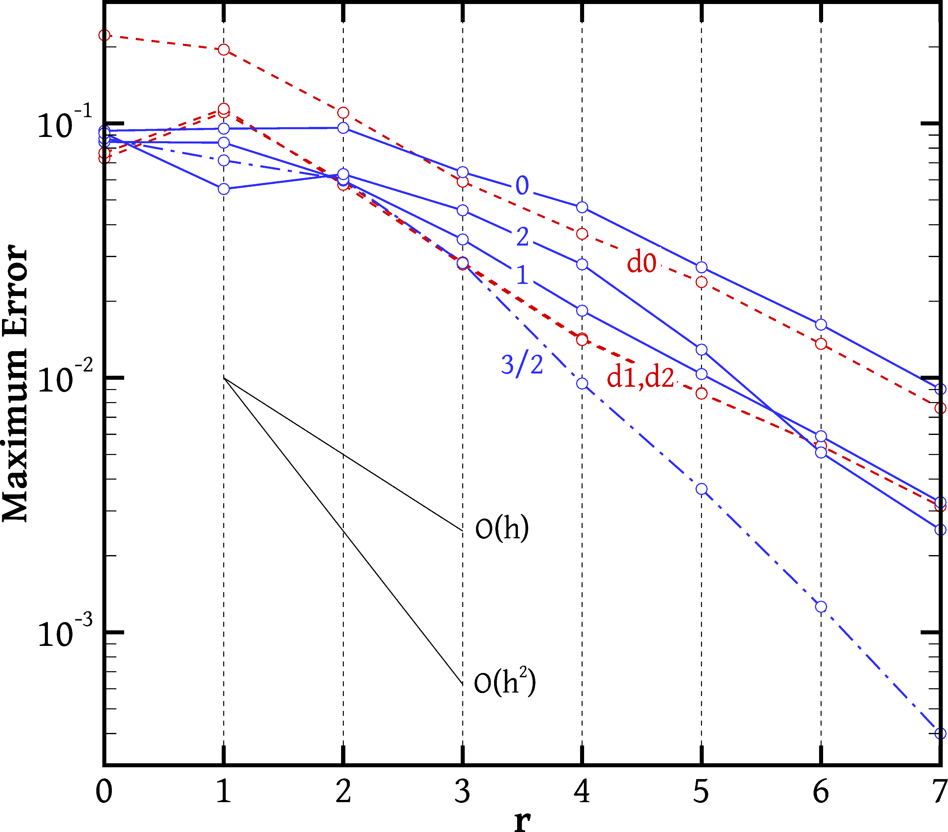
(b) maximum error, $\tau_{\mathrm{max}}$

Figure 10: The mean 10(a) and maximum 10(b) errors (defined by Eqs. (36) and (37), respectively) of the gradient schemes applied on the function $\phi=\tanh(x)\tanh(y)$ on smooth curvilinear grids (Fig. 9). The abscissa $r$ designates the grid; $r=0$ is the coarsest grid (Fig. 9(a)), and grid $r$ comes from subdividing every cell of grid $r-1$ into 4 child cells in the computational space (see text). The blue solid lines correspond to the LS methods with $q$ = 0, 1 and 2 as indicated on each curve; the blue dash-dot line corresponds to the LS method with $q=3/2$; and the red dashed lines correspond to the DT methods $\mathrm{d}c$ where $c$ is the number of corrector steps.

These grids exhibit all kinds of grid irregularity, but the unevenness and the skewness diminish with grid refinement, as explained in Section 2. In particular, Table 1 shows that the measures of both these grid qualities have magnitudes of $O(h)$. These measures were defined in Sec. 2: $\|\bm{c}^{\prime}_{f}-\bm{m}_{f}\|/\|\bm{N}_{f}-\bm{P}\|$ for unevenness and $\|\bm{c}_{f}-\bm{c}^{\prime}_{f}\|/\|\bm{N}_{f}-\bm{P}\|$ for skewness (see Fig 1 for definitions). The values listed in Table 1 are the average values among all faces of each grid, excluding boundary faces. Therefore, it is expected that eventually the methods will behave as in the Cartesian case. Indeed, Fig. 10(b) shows that as the grid is refined $\tau_{\mathrm{max}}$ tends to decrease at a first-order rate for all methods, except for the least squares method with $q=3/2$, for which it decreases at a second-order rate. Accordingly, Fig. 10(a) shows that $\tau_{\mathrm{mean}}$ tends to decrease at a second-order rate for all methods, with the second-order rate attained earlier by the $q=3/2$ method. Therefore, like on the Cartesian grids, the methods are second-order accurate at interior cells but revert to first-order accuracy at boundary cells, except for the $q=3/2$ method.

Of the LS methods the least accurate is the unweighted method, followed by the $q=2$ method. The undisputed champion is the $q=3/2$ method because, as mentioned, it retains its second-order accuracy even at boundary cells. Concerning the DT methods, the method with no corrections (Eq. 10) performs similarly to the unweighted LS method. Application of a corrector step (Eq. (17)) now does make a difference, since skewness is present at any finite grid density, bringing the accuracy of the method on a par with the best weighted LS methods, except of course the $q=3/2$ method. We also tried a second corrector step but it did not bring any noticeable improvement.

Next, on the same grids we also applied discrete gradient operators to calculate the gradient of a linear and of a quadratic function. The schemes tested are the DT gradient operators $\nabla^{\mathrm{d}0}$, $\nabla^{\mathrm{d}1}$ and $\nabla^{\mathrm{d}\infty}$ (the latter approximated with 100 correction steps), and the LS gradient operators with $q$ = 0, 1 and 3/2, denoted as $\nabla^{\mathrm{ls}0}$, $\nabla^{\mathrm{ls}1}$ and $\nabla^{\mathrm{ls}3/2}$, respectively, in Tables 1 and 2. “Exactness” is sometimes used as an aid to either determine the order of accuracy of a method or to design a method to achieve a desired order of accuracy (e.g. Appendix B): a first-order accurate gradient scheme would normally be exact for linear functions, and a second-order accurate gradient scheme would normally be exact for quadratic functions. However, the results listed in Tables 1 and 2 show that in the present case the DT gradient is not exact even for linear functions while the LS gradient is exact for linear functions but not for quadratic functions, despite both methods being second-order accurate.

In particular, Table 1 shows that the DT gradient without corrector steps ($\nabla^{\mathrm{d}0}$) is not exact for the linear function (the errors are not zero) but converges to the exact gradient at a rate that approaches second-order as the grid is refined. Performing a corrector step ($\nabla^{\mathrm{d}1}$) brings a significant improvement in accuracy, with an observed convergence rate order of between 2 and 3, but still the operator is not exact. This inexactness is anticipated since the grids are skewed and the DT scheme cannot cope with skewness. However, grid refinement causes skewness to diminish and the DT accuracy to improve at a second-order rate. In the limit of many corrector steps ($\nabla^{\mathrm{d}\infty}$) the operator becomes exact, with the errors at machine precision levels even at the coarsest grid. All of the LS schemes are also exact for the linear function.

Concerning the quadratic function (Table 2), none of the schemes is exact but they are all second-order accurate, with the $q=3/2$ LS scheme being the most accurate, and the $q=0$ LS and zero-correction DT schemes being the least accurate. A single corrector step in the DT scheme ($\nabla^{\mathrm{d}1}$) brings the maximum attainable improvement, since the error levels of $\nabla^{\mathrm{d}1}$ and $\nabla^{\mathrm{d}\infty}$ are nearly identical. The second-order convergence rates are due to the improvement of grid quality with refinement, as explained in Sections 3 and 4.

Table 1: Mean errors (Eq. (36)) of various schemes for calculating the gradient $\nabla\phi=(1,2)$ of the linear function $\phi(x,y)=x+2y+0.5$ on the series of grids shown in Fig. 9. Also displayed are the measures of grid skewness and unevenness (defined in Sec. 2), averaged over all faces of each grid excluding boundary faces.

Grid $r$	Skew.	Unev.	$\nabla^{\mathrm{d}0}$	$\nabla^{\mathrm{d}1}$	$\nabla^{\mathrm{d}\infty}$	$\nabla^{\mathrm{ls}0}$	$\nabla^{\mathrm{ls}1}$	$\nabla^{\mathrm{ls}3/2}$
0	1.33$\cdot 10^{-1}$	1.10$\cdot 10^{-1}$	4.16$\cdot 10^{-1}$	8.00$\cdot 10^{-2}$	2.19$\cdot 10^{-15}$	6.04$\cdot 10^{-16}$	7.39$\cdot 10^{-16}$	9.37$\cdot 10^{-16}$
1	5.68$\cdot 10^{-2}$	8.00$\cdot 10^{-2}$	1.86$\cdot 10^{-1}$	1.90$\cdot 10^{-2}$	4.46$\cdot 10^{-15}$	1.34$\cdot 10^{-15}$	1.45$\cdot 10^{-15}$	1.68$\cdot 10^{-15}$
2	3.03$\cdot 10^{-2}$	4.83$\cdot 10^{-2}$	6.93$\cdot 10^{-2}$	4.80$\cdot 10^{-3}$	9.53$\cdot 10^{-15}$	2.43$\cdot 10^{-15}$	2.41$\cdot 10^{-15}$	2.81$\cdot 10^{-15}$
3	1.64$\cdot 10^{-2}$	2.70$\cdot 10^{-2}$	2.41$\cdot 10^{-2}$	8.91$\cdot 10^{-4}$	1.93$\cdot 10^{-14}$	4.42$\cdot 10^{-15}$	4.52$\cdot 10^{-15}$	4.84$\cdot 10^{-15}$
4	8.44$\cdot 10^{-3}$	1.43$\cdot 10^{-2}$	7.72$\cdot 10^{-3}$	1.16$\cdot 10^{-4}$	3.97$\cdot 10^{-14}$	8.74$\cdot 10^{-15}$	8.77$\cdot 10^{-15}$	9.07$\cdot 10^{-15}$
5	4.29$\cdot 10^{-3}$	7.41$\cdot 10^{-3}$	2.32$\cdot 10^{-3}$	1.43$\cdot 10^{-5}$	7.98$\cdot 10^{-14}$	1.70$\cdot 10^{-14}$	1.71$\cdot 10^{-14}$	1.74$\cdot 10^{-14}$
6	2.16$\cdot 10^{-3}$	3.78$\cdot 10^{-3}$	6.64$\cdot 10^{-4}$	1.94$\cdot 10^{-6}$	1.60$\cdot 10^{-13}$	3.36$\cdot 10^{-14}$	3.38$\cdot 10^{-14}$	3.40$\cdot 10^{-14}$
7	1.09$\cdot 10^{-3}$	1.91$\cdot 10^{-3}$	1.86$\cdot 10^{-4}$	3.25$\cdot 10^{-7}$	3.20$\cdot 10^{-13}$	6.69$\cdot 10^{-14}$	6.70$\cdot 10^{-14}$	6.72$\cdot 10^{-14}$

Table 2: Mean errors (Eq. (36)) of various schemes for calculating the gradient $\nabla\phi=(2x+2y,2x-2y)$ of the quadratic function $\phi(x,y)=x^{2}+2xy-y^{2}$ on the series of grids shown in Fig. 9.

Grid $r$	$\nabla^{\mathrm{d}0}$	$\nabla^{\mathrm{d}1}$	$\nabla^{\mathrm{d}\infty}$	$\nabla^{\mathrm{ls}0}$	$\nabla^{\mathrm{ls}1}$	$\nabla^{\mathrm{ls}3/2}$
0	4.95$\cdot 10^{-1}$	2.28$\cdot 10^{-1}$	2.29$\cdot 10^{-1}$	3.54$\cdot 10^{-1}$	1.94$\cdot 10^{-1}$	1.47$\cdot 10^{-1}$
1	2.20$\cdot 10^{-1}$	1.27$\cdot 10^{-1}$	1.29$\cdot 10^{-1}$	1.72$\cdot 10^{-1}$	8.16$\cdot 10^{-2}$	5.81$\cdot 10^{-2}$
2	8.38$\cdot 10^{-2}$	4.48$\cdot 10^{-2}$	4.47$\cdot 10^{-2}$	8.09$\cdot 10^{-2}$	3.13$\cdot 10^{-2}$	2.24$\cdot 10^{-2}$
3	2.84$\cdot 10^{-2}$	1.46$\cdot 10^{-2}$	1.46$\cdot 10^{-2}$	3.20$\cdot 10^{-2}$	1.12$\cdot 10^{-2}$	7.43$\cdot 10^{-3}$
4	8.99$\cdot 10^{-3}$	4.63$\cdot 10^{-3}$	4.64$\cdot 10^{-3}$	1.14$\cdot 10^{-2}$	3.76$\cdot 10^{-3}$	2.05$\cdot 10^{-3}$
5	2.66$\cdot 10^{-3}$	1.40$\cdot 10^{-3}$	1.40$\cdot 10^{-3}$	3.75$\cdot 10^{-3}$	1.19$\cdot 10^{-3}$	5.28$\cdot 10^{-4}$
6	7.45$\cdot 10^{-4}$	4.00$\cdot 10^{-4}$	4.01$\cdot 10^{-4}$	1.15$\cdot 10^{-3}$	3.50$\cdot 10^{-4}$	1.35$\cdot 10^{-4}$
7	2.07$\cdot 10^{-4}$	1.10$\cdot 10^{-4}$	1.10$\cdot 10^{-4}$	3.29$\cdot 10^{-4}$	9.74$\cdot 10^{-5}$	3.41$\cdot 10^{-5}$

5.4 Grids of localised high distortion

Structured grids that are constructed not by solving partial differential equations, as in Section 5.3, but by algebraic methods may lack the property that unevenness and skewness diminish with grid refinement. This is especially true if the domain boundaries include sharp corners at points other than grid line endpoints. For example, the grid of Fig. 11 is structured, consisting of piecewise straight lines. At the line joining the sharp corners, the intersecting grid lines change direction abruptly. This causes significant skewness which is unaffected by grid refinement.

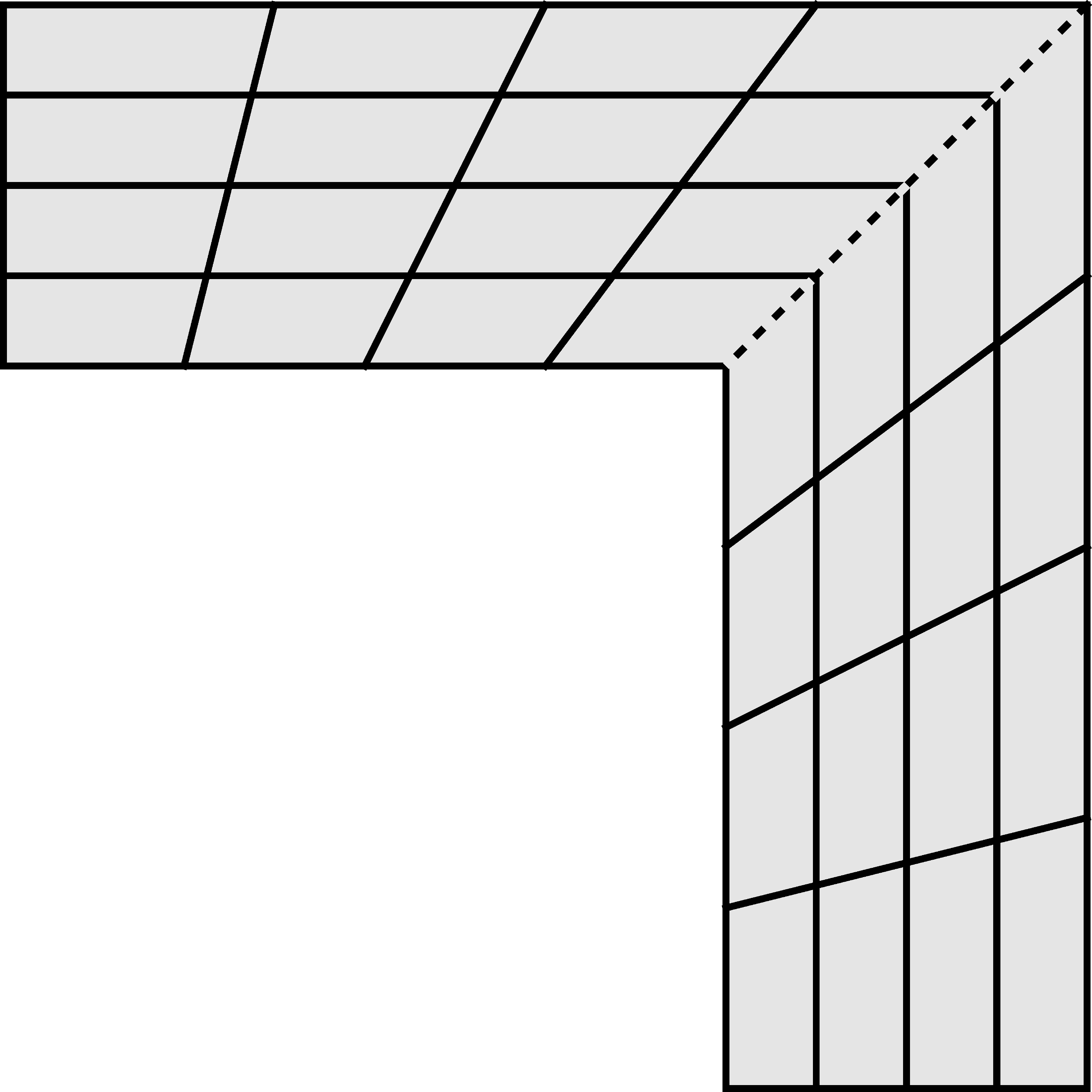
Figure 11: A structured grid where the grid lines belonging to one family change direction abruptly at the dashed line joining the pair of sharp corners, where grid skewness and not diminishing with grid refinement.

A similar situation may occur when adaptive mesh refinement is used, depending on the treatment of the interaction between levels. Figure 12 shows multi-level grids, which consist of regions of different fineness. Such grids are often called composite grids [35]. One possible strategy is to treat the cells at the level interfaces as topologically polygonal [29, 8, 36]. For example, cell $P$ of Fig. 13(a) has 6 faces, each separating it from a single other cell. Its face $f_{1}$ separates it from cell $N_{1}$ which belongs to the finer level. Faces such as $f_{1}$, which lie on grid level interfaces, exhibit non-orthogonality, unevenness, and skewness. If the grid density is increased throughout the domain, as in the series of grids shown in Fig. 12, then these interface distortions remain insensitive to the grid fineness, like for the marked line in Fig. 11. Alternative schemes exist which avoid changing the topology of the cells by inserting a layer of transitional cells between the coarse and the fine part of the grid (e.g. [37, 38]) but they also lead to high, non-diminishing grid distortions at the interface.

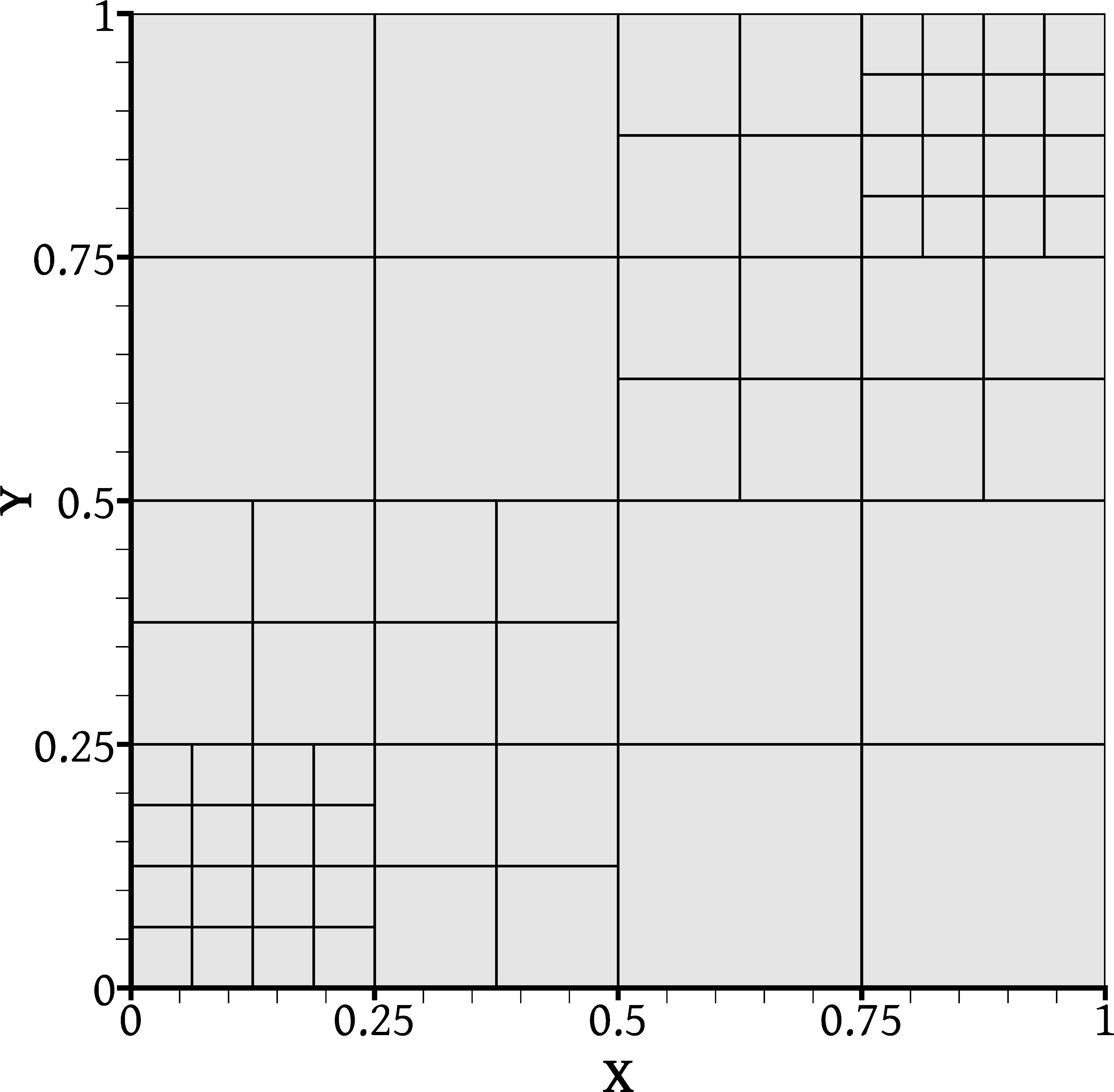
(a) $r=0$

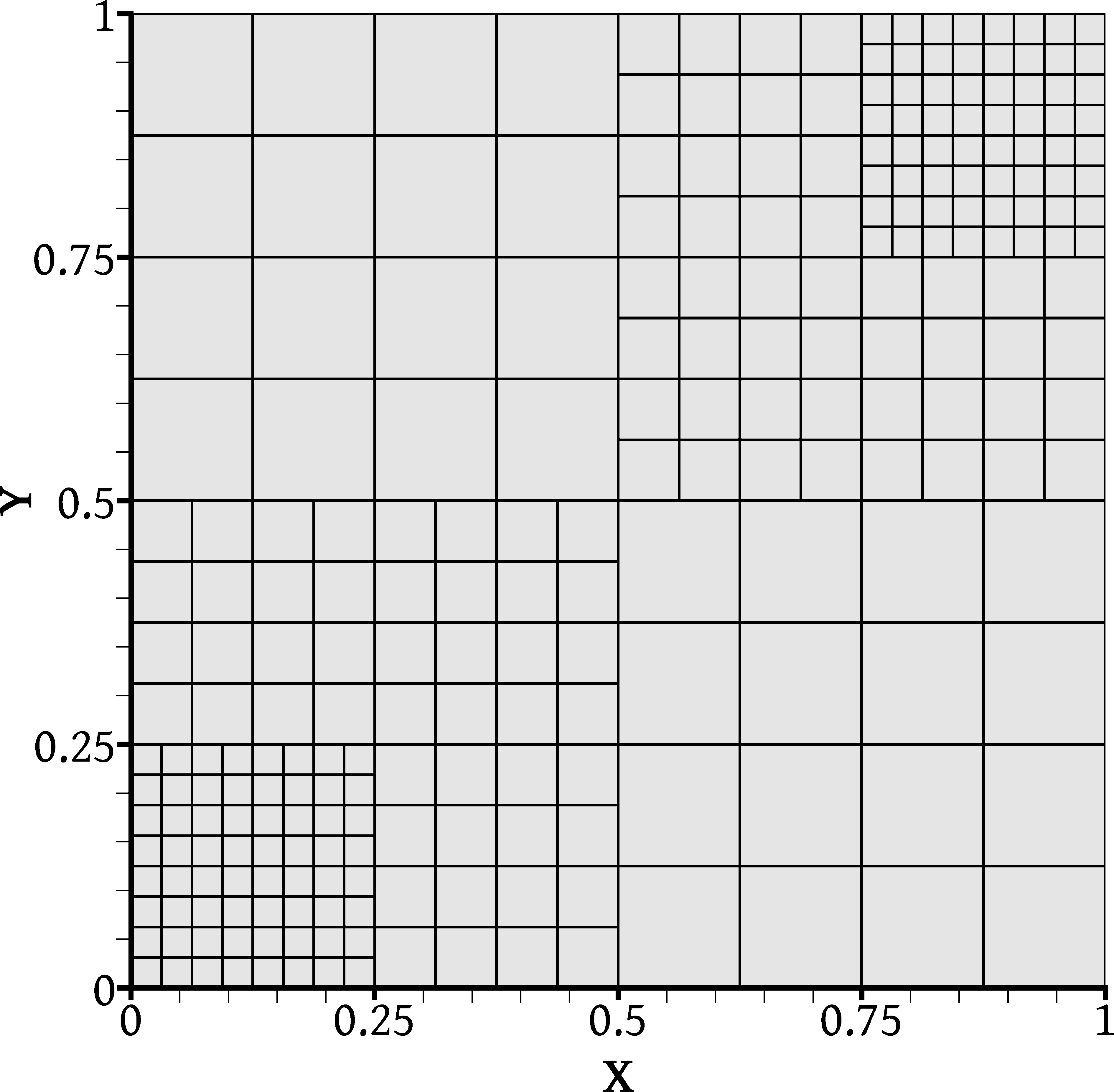
(b) $r=1$

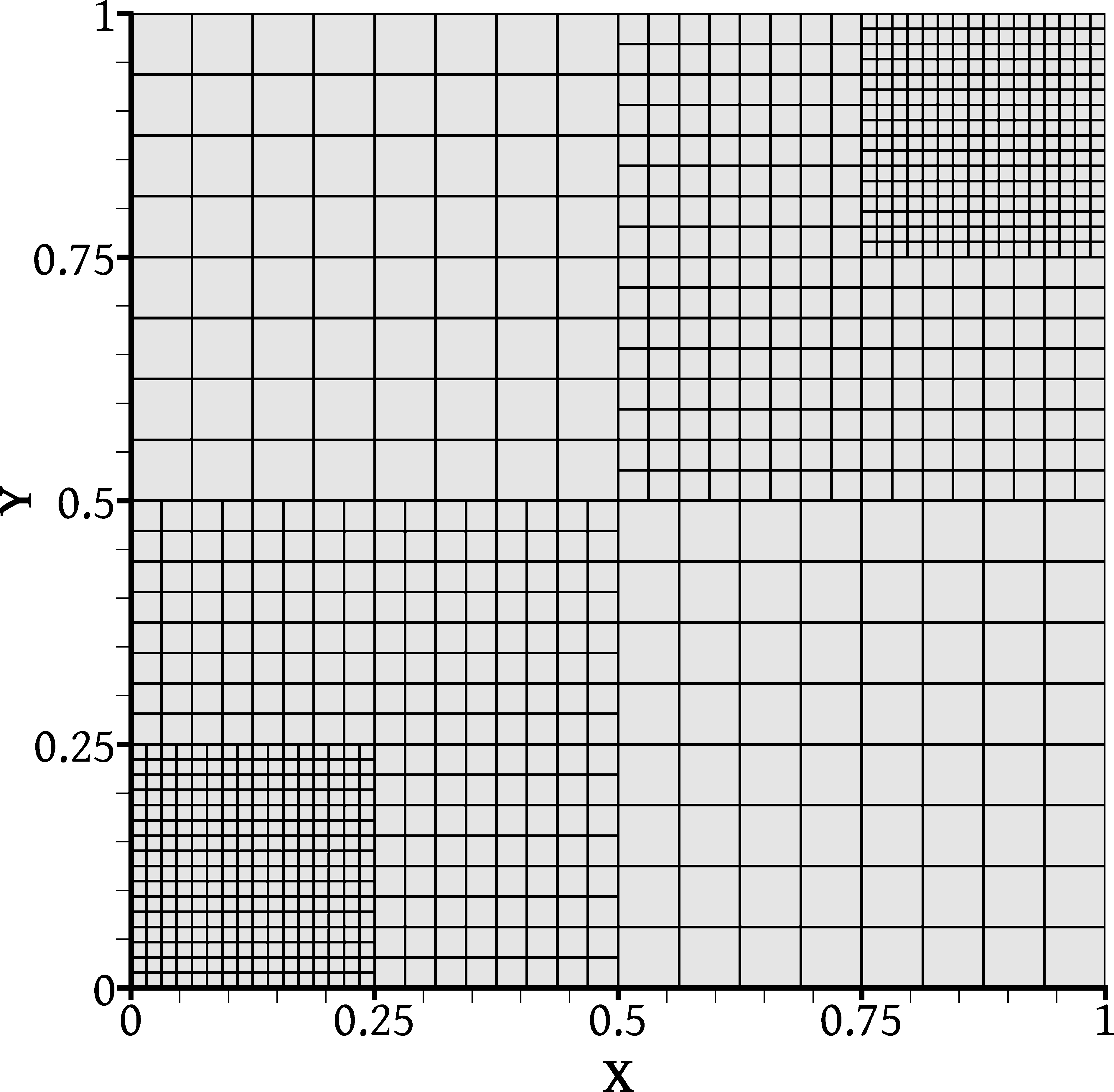
(c) $r=2$

Figure 12: A series of multi-level, or composite, grids. Each grid $r$ comes from the previous grid $r-1$ by evenly subdividing each cell into four child cells.

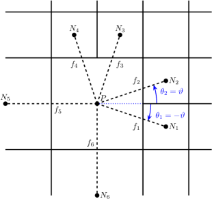
(a) coarse cell

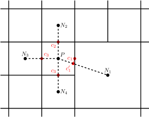
(b) fine cell

Figure 13: Topological and geometrical characteristics of a coarse cell 13(a) and of a fine cell 13(b) adjacent to a level interface, in a composite grid.

We computed the gradient of the same function $\phi(x,y)=\tanh(x)\tanh(y)$ on a series of composite grids the first three of which are shown in Fig. 12. Figure 14 shows how $\tau_{\mathrm{mean}}$ and $\tau_{\mathrm{max}}$ vary with grid refinement. This time, $\tau_{\mathrm{mean}}$ is defined a little differently than Eq. (36) to account for the different grid levels: the error of each individual cell is weighted by the cell’s volume (i.e. the area, in the present two-dimensional setting):

$$\tau_{\mathrm{mean}}\;\equiv\;\frac{1}{\Omega}\sum_{P=1}^{M_{r}}\Omega_{P}\|\nabla^{\mathrm{a}}\phi(\bm{P})-\nabla\phi(\bm{P})\|$$ (38)

where $\Omega$ is the total volume of the domain and $\Omega_{P}$ is the volume of cell $P$.

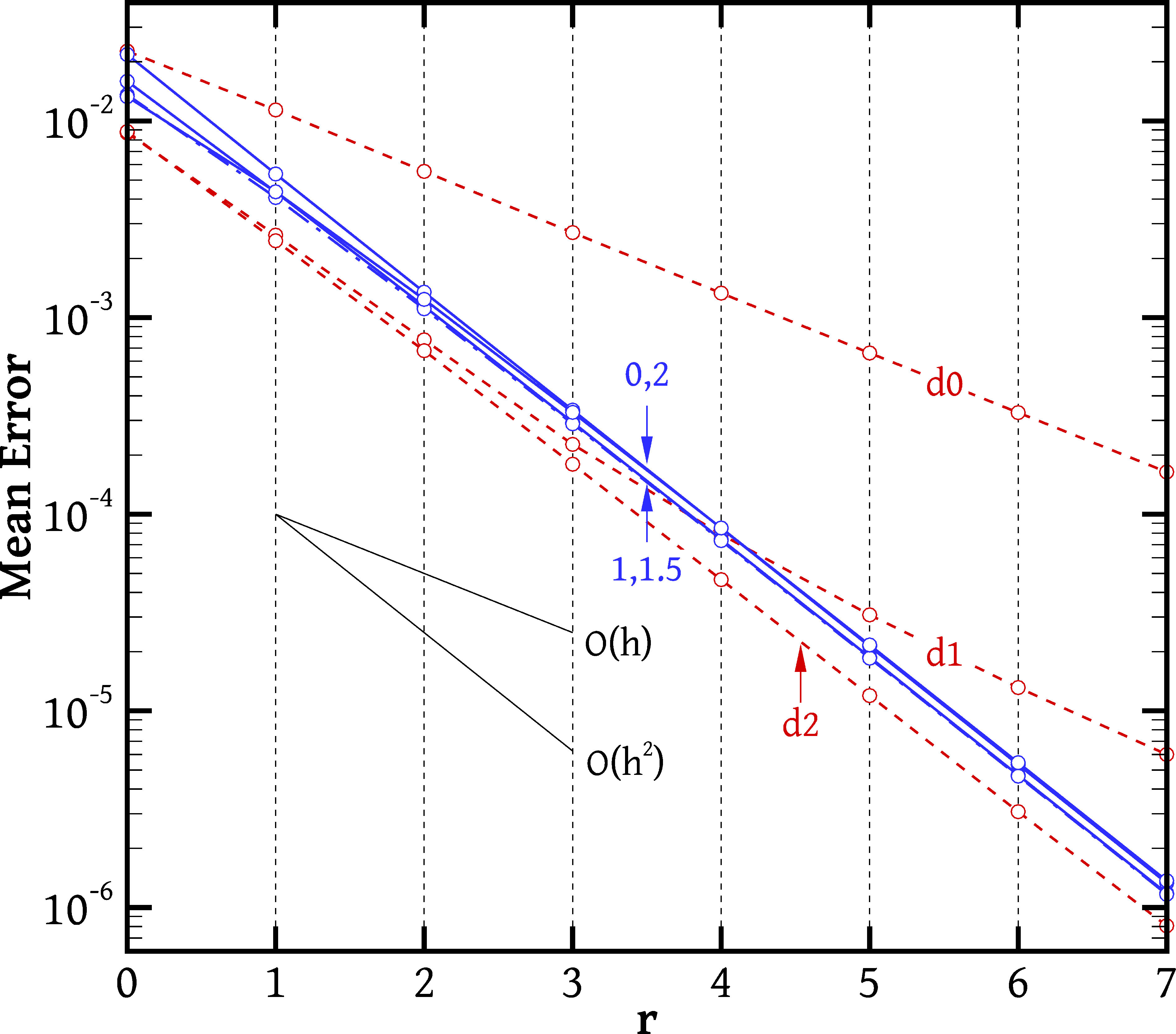
(a) mean error, $\tau_{\mathrm{mean}}$

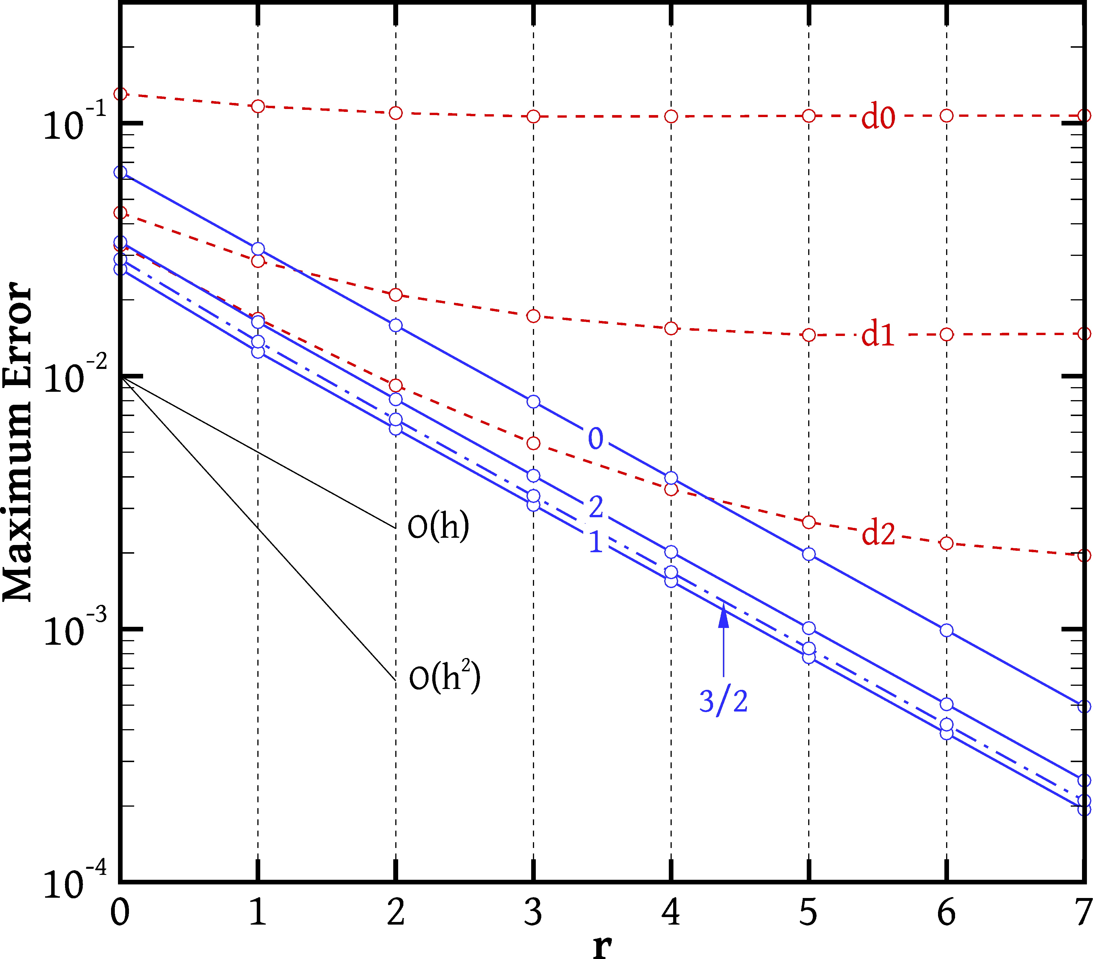
(b) maximum error, $\tau_{\mathrm{max}}$

Figure 14: The mean 14(a) and maximum 14(b) errors (defined by Eqs. (38) and (37), respectively) of the gradient calculation methods applied to the function $\phi=\tanh(x)\tanh(y)$ on locally refined grids (Fig. 12). The abscissa $r$ designates the grid; $r=0$ is the coarsest grid (Fig. 12(a)), and grid $r$ comes from subdividing every cell of grid $r-1$ into 4 identical child cells. The blue solid lines correspond to the LS methods with weight exponents $q$ = 0, 1 and 2, which are indicated on each curve; the blue dash-dot line corresponds to the LS method with $q=3/2$; and the red dashed lines correspond to the DT methods $\mathrm{d}c$ where $c$ is the number of corrector steps.

We can identify three classes of cells that are topologically different. Apart from the familiar classes of interior and boundary cells, there is now also the class of cells that touch the level interfaces, which shall be called interface cells (these belong to two sub-classes, coarse- and fine-level cells, as in Figs. 13(a) and 13(b), respectively). Interface cells possess high skewness and unevenness that do not diminish with grid refinement. The behaviour of the gradient-calculation methods at interior and boundary cells has already been tested in Sections 5.2 and 5.3, so our interest now focuses on interface cells. Skewness, the most detrimental grid distortion, is encountered only at those and therefore it is there that the maximum errors (Fig. 14(b)) occur.

In Fig. 14(b) we observe that at the level interfaces all the LS methods converge to the correct solution at a first-order rate, $\tau_{\mathrm{max}}$ being lowest for the $q=1$ method, followed closely by the $q=3/2$ and $q=2$ methods. On the other hand, none of the DT methods converge to the correct solution there, although nearly an order of magnitude accuracy improvement is obtained with each corrector step. We can determine the operator to whom $\nabla^{\mathrm{d}0}$ converges as follows. For the interface cell $P$ of Fig. 13(b), formula (10) amounts to the following series of approximations:

$$\phi_{\!.x}(\bm{P})\; \approx\;\frac{\phi(\bm{c}_{1})-\phi(\bm{c}_{3})}{h}\;\approx\;\frac{\phi(\bm{c}^{\prime}_{1})-\phi(\bm{c}_{3})}{h}$$

$$\approx\;\frac{\left[\alpha\,\phi(\bm{N}_{1})+(1-\alpha)\,\phi(\bm{P})\right]\;-\;\left[0.5\,\phi(\bm{P})+0.5\,\phi(\bm{N}_{3})\right]}{h}\;\equiv\;\phi_{\!.x}^{\mathrm{d}0}(\bm{P})$$ (39)

where $h$ is the length of the side of cell $P$. In the last step, the values of $\phi$ at points $\bm{c}^{\prime}_{1}$ and $\bm{c}_{3}$ were approximated with linear interpolation between points $\bm{N}_{1}$ and $\bm{P}$, and $\bm{P}$ and $\bm{N}_{3}$, respectively; $\alpha$ is an interpolation factor which equals $\alpha=0.3$ for the present geometry. We then substitute in (39) $\phi(\bm{N}_{1})$ and $\phi(\bm{N}_{3})$ with their two-dimensional Taylor series about $\bm{P}$, considering that if $\bm{P}=(x_{0},\,y_{0})$ then $\bm{N}_{1}=(x_{0}\!+\!3h/2,\,y_{0}\!-\!h/2)$ and $\bm{N}_{3}=(x_{0}\!-\!h,\,y_{0})$ – see Fig. 13(b). The following result is obtained:

$$\phi_{\!.x}^{\mathrm{d}0}(\bm{P})\;=\;\frac{3\alpha+1}{2}\,\phi_{\!.x}(\bm{P})\;-\;\frac{\alpha}{2}\,\phi_{\!.y}(\bm{P})\;+\;O(h)$$

Therefore, as $h\rightarrow 0$, $\phi_{\!.x}^{\mathrm{d}0}$ converges not to $\phi_{\!.x}$ but to an operator that involves both $\phi_{\!.x}$ and $\phi_{\!.y}$.

Next we examine the mean error in Fig. 14(a). The plot can be interpreted by considering separately the error contributions of each class of cells. The contributions of interior and boundary cells to $\tau_{\mathrm{mean}}$ are both $O(h^{2})$, as discussed in Section 5.2 (for the $q=3/2$ method the boundary cell contribution is $O(h^{3})$).

At interface cells the LS methods behave similarly as on boundary cells, because they produce $O(h)$ errors there as well due to unevenness and skewness. The total length of the level interfaces is constant, $O(1)$. The number of interface cells is $O(h^{-1})$ because it equals this constant length divided by the cell size which is $O(h)$. Their contribution to the mean error in Eq. (38) is (number of cells) $\times$ (volume of one cell) $\times$ (error at a cell) = $O(h^{-1})\times O(h^{2})\times O(h)=O(h^{2})$. This is confirmed by Fig. 14(a), where all the LS methods converge to the exact solution at a second-order rate.

On the other hand, for the DT methods the contribution of interface cells to $\tau_{\mathrm{mean}}$ is (number of cells) $\times$ (volume of one cell) $\times$ (error at a cell) = $O(h^{-1})\times O(h^{2})\times O(1)=O(h)$. Figure 14(a) shows that for the d0 method (no corrector steps) this $O(h)$ component is so large that it dominates $\tau_{\mathrm{mean}}$ even at coarse grids. For the d1 method (one corrector step), at coarse grids this $O(h)$ component is initially small compared to the bulk $O(h^{2})$ component that comes from all the other cells, so that $\tau_{\mathrm{mean}}$ appears to decrease at a second-order rate up to a refinement level of $r=3$; but eventually it becomes dominant and beyond $r=5$ the d1 curve is parallel to the d0 curve, with a first-order slope. With two corrector steps, the $O(h)$ component is so small that up to $r=7$ it is completely masked by the $O(h^{2})$ component and the method appears to be second-order accurate. More grid refinements are necessary to reveal its asymptotic first-order accuracy.

An observation that raises some concern in Fig. 14(a) is that the DT methods outperform the LS methods at those grids where they have not yet degraded to first order. This suggests that there may be some room for improvement in the latter. A potential source of the problem is suggested by Fig. 13(a). Along the horizontal direction, cell $P$ has one cell on its left side ($N_{5}$) and two cells on its right side ($N_{1}$ and $N_{2}$). Since points $\bm{N}_{1}$ and $\bm{N}_{2}$ are quite close to each other there is some overlap in the information they convey. Yet the weights of the LS method depend only on the distance of $\bm{N}_{f}$ from $\bm{P}$, while any clustering of the $\bm{N}_{f}$ points in some direction is not taken into account. Thus, points $\bm{N}_{1}$ and $\bm{N}_{2}$, being closer to $\bm{P}$ than $\bm{N}_{5}$ may individually contribute equally ($q=1$) or more ($q>1$) to the calculation of the gradient at $\bm{P}$ than point $\bm{N}_{5}$ does. Combined they contribute much more. So, the horizontal component of the gradient is calculated using mostly information from the right of cell $P$, whereas information from its left is undervalued. The DT methods do not suffer from this deficiency because they weigh the contribution of each point by the area of the respective face; faces $f_{1}$ and $f_{2}$ are half in size than $f_{5}$, and so points $\bm{N}_{1}$ and $\bm{N}_{2}$ together contribute to the gradient approximately as much as $\bm{N}_{5}$ alone does.

In order to seek a remedy, we investigate the contributions of points $\bm{N}_{1}$, $\bm{N}_{2}$ and $\bm{N}_{5}$ (Fig. 13(a)) to the vector $\beta_{\varsigma}$ of the error expression (31). As for Eq. (35), we substitute for $\varsigma_{f}$ from Eq. (25) into the expression for $\beta_{\varsigma}$, but then proceed to substitute $\Delta x_{f}=\Delta r_{f}\cos\theta_{f}$, $\Delta y_{f}=\Delta r_{f}\sin\theta_{f}$. For the particular points under consideration we have, with reference to Fig. 13(a), $\theta_{1}=-\vartheta$, $\theta_{2}=\vartheta$ and $\theta_{5}=\pi$, while $\Delta r_{2}=\Delta r_{1}$. Finally, concerning the weights, since cells $P$ and $N_{5}$ both belong to the same grid level we choose not to tamper with the weight $w_{5}$ and simply use the possibly second-order accurate $q=3/2$ scheme: $w_{5}=(\Delta r_{5})^{-3/2}$. Due to symmetry we set $w_{2}=w_{1}$ and our goal is to suitably select $w_{1}$ to achieve a small error. Putting everything together, the joint contribution of these three points to $\beta_{\varsigma}$ is, neglecting higher order terms,

$$\begin{bmatrix}\phi_{\!.xx}\left(\left(\cos\vartheta\right)^{3}(\Delta r_{1})^{3}\,w_{1}^{2}\,-\,\frac{1}{2}\right)\;+\;\phi_{\!.yy}\left(\sin\vartheta\right)^{2}\cos\vartheta\,(\Delta r_{1})^{3}\,w_{1}^{2}\\[11.38092pt] 2\phi_{\!.xy}\,\cos\vartheta\left(\sin\vartheta\right)^{2}(\Delta r_{1})^{3}\,w_{1}^{2}\end{bmatrix}$$ (40)

Since the values of the higher order derivatives can be arbitrary, it is obvious that the above contribution does not become zero for any choice of $w_{1}$; thus, second-order accuracy cannot be achieved. The best that can be done is to choose $w_{1}=(\cos\vartheta)^{-3/2}(\Delta r_{1})^{-3/2}/\sqrt{2}$ so that the term in parentheses multiplied by $\phi_{.xx}$ becomes zero. In fact, since this choice is not guaranteed to minimise the error and since $\cos\vartheta\approx 1$ for relatively small $\vartheta$, we chose to drop the $\cos\vartheta$ factor and applied the following scheme to all least squares methods:

$$w_{f}\;=\;\begin{cases}\|\bm{N}_{f}-\bm{P}\|^{-q}&\qquad\text{face }f\text{ does not touch a finer level}\\ \frac{1}{\sqrt{2}}\|\bm{N}_{f}-\bm{P}\|^{-q}&\qquad\text{face }f\text{ touches a finer level}\end{cases}$$ (41)

(In the three-dimensional case, cell $P$ of Fig. 13(a) would have four fine-level neighbours on its right and the $1/\sqrt{2}$ factor in (41) would become $1/\sqrt{4}=1/2$). Using this scheme, we obtained the results shown in Fig. 15, which can be seen to be better than those of Fig. 14, especially for the $q=3/2$ and $q=2$ methods which now rival the d2 method with respect to the mean error.

(a) mean error, $\tau_{\mathrm{mean}}$

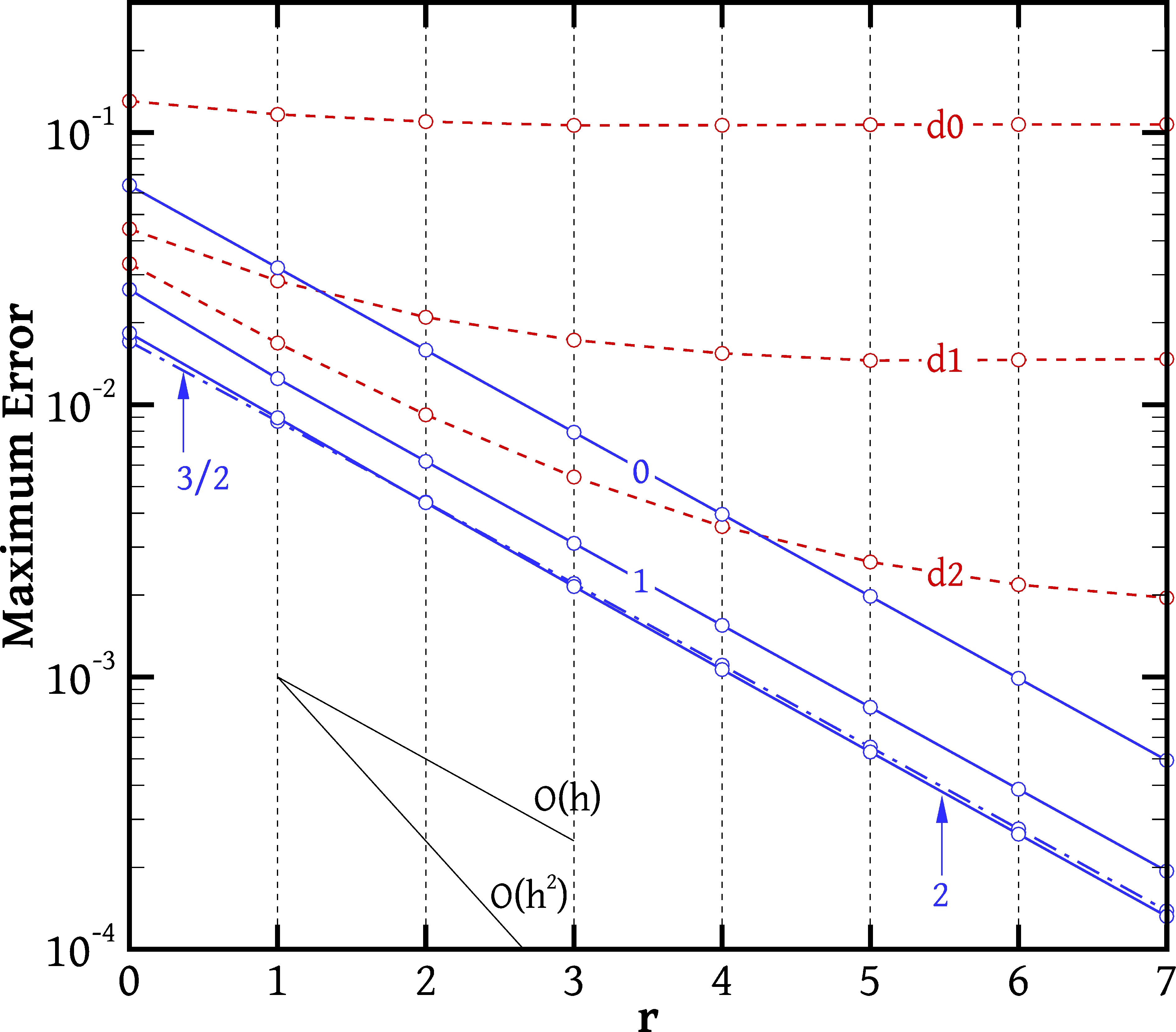
(b) maximum error, $\tau_{\mathrm{max}}$

Figure 15: As for Fig. 14, but with the weights (41) applied at level interfaces in the case of the LS methods.

The modification (41) is easy and inexpensive. More elaborate methods could be devised, applicable to more general grid configurations, in order to properly deal with the issue of point clustering at certain angles. For example, a point $\bm{N}_{f}$ could be assigned to span a “sector” of angle $\Delta\theta_{f}=|\theta_{f+1}-\theta_{f-1}|/2$ (assuming that the points are numbered in either clockwise or anti-clockwise order); the sum of all these sectors would then equal $2\pi$, and they could be incorporated into the weights such that points with smaller sectors would have less influence over the solution. Alternatively, the face areas could be incorporated into the weights, as in the DT method [18].

5.5 Grids with arbitrary distortion

As mentioned in Section 3, general-purpose unstructured grid generation methods result in unevenness and skewness that are insensitive to grid fineness throughout the domain, not just in isolated regions as for the grids of Section 5.4. Therefore, in the present Section the methods are tested under these conditions; grids of non-diminishing distortion were generated by randomly perturbing the vertices of a Cartesian grid. Using such a process we constructed a series of grids, the first three of which are shown in Fig. 16. The perturbation procedure is applied as follows: Suppose a Cartesian grid with grid spacing $h$. If node $(i,j)$ has coordinates $(x_{ij},\,y_{ij})$ then the perturbation procedure moves it to a location $(x^{\prime}_{ij},\,y^{\prime}_{ij})=(x_{ij}+\delta^{x}_{ij},\,y_{ij}+\delta^{y}_{ij})$ where $\delta^{x}_{ij}$ and $\delta^{y}_{ij}$ are random numbers in the interval $[-0.25h,0.25h)$. Because all perturbations are smaller than $h/4$ in both $x$ and $y$, it is ensured that all grid cells remain simple convex quadrilaterals after all vertices have been perturbed. Grids based on triangles as well as three-dimensional cases will be considered in Section 6.

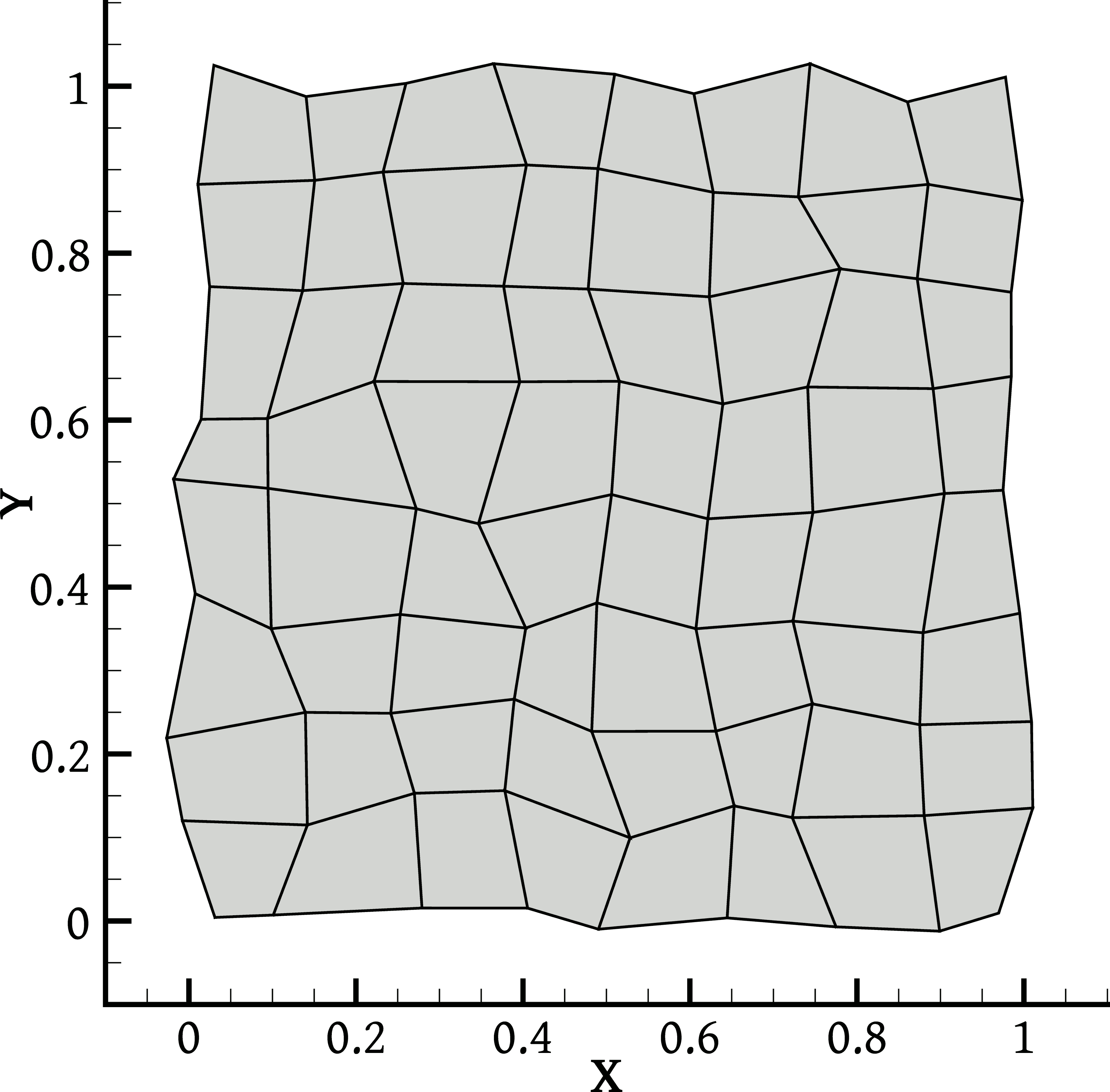
(a) $r=0$

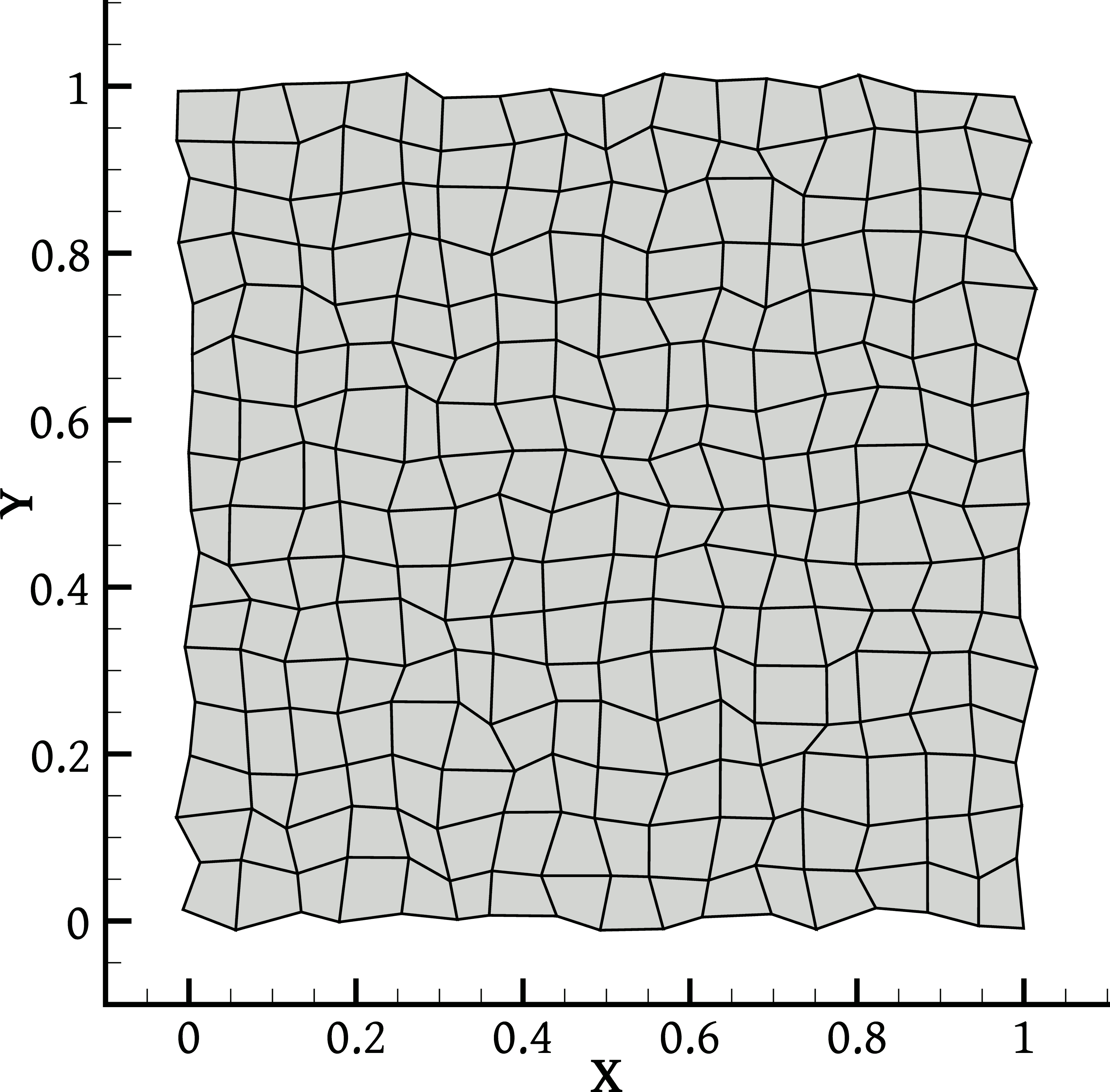
(b) $r=1$

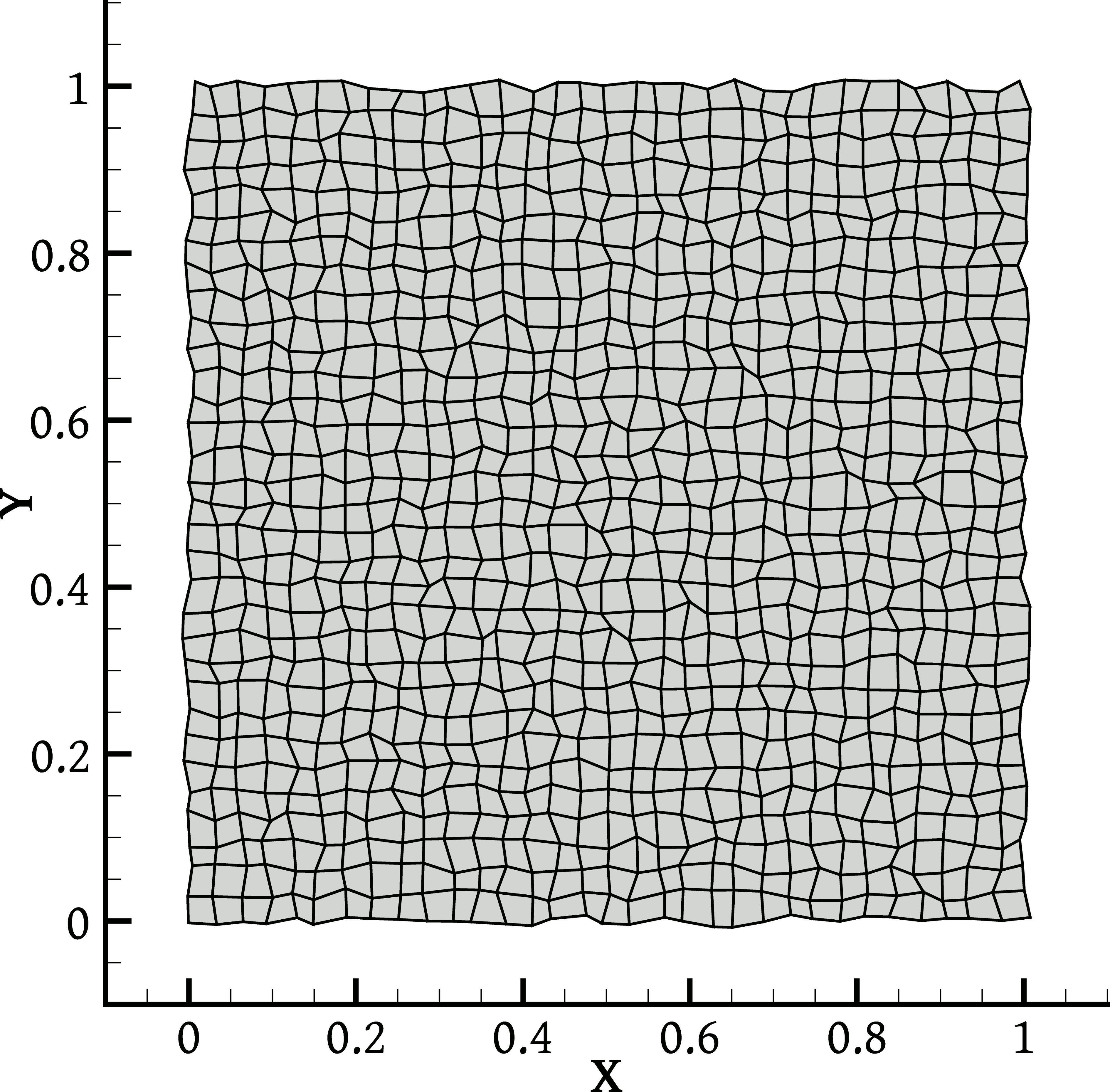
(c) $r=2$

Figure 16: A series of excessively distorted grids. Grid $r$ is constructed by random perturbation of the nodes of Cartesian grid $r+1$ of Section 5.2.

The gradient of the same function $\phi=\tanh(x)\tanh(y)$ is calculated, and the errors are plotted in Fig. 17. This time, all cells belong to a common category. Concerning the mean error, Fig. 17(a) is in full agreement with the theory. The LS methods converge to the exact gradient at a first-order rate, with the unweighted method being, as usual, the least accurate, while the differences between the weighted methods are very slight. On the other hand, the DT methods, as expected, do not converge to the exact gradient. Performing corrector steps improves things, but in every case the convergence eventually stagnates at some grid fineness.

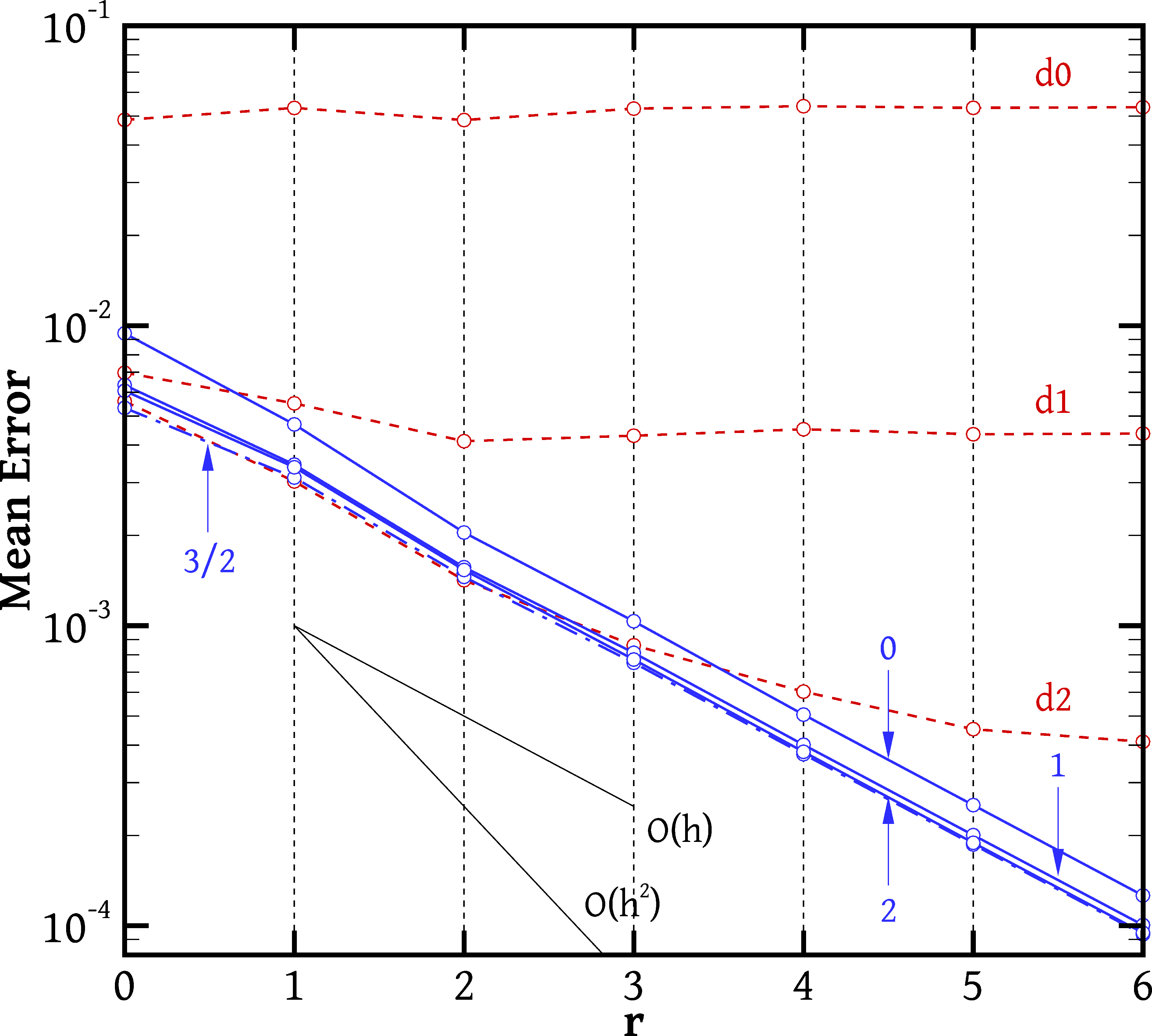
(a) mean error, $\tau_{\mathrm{mean}}$

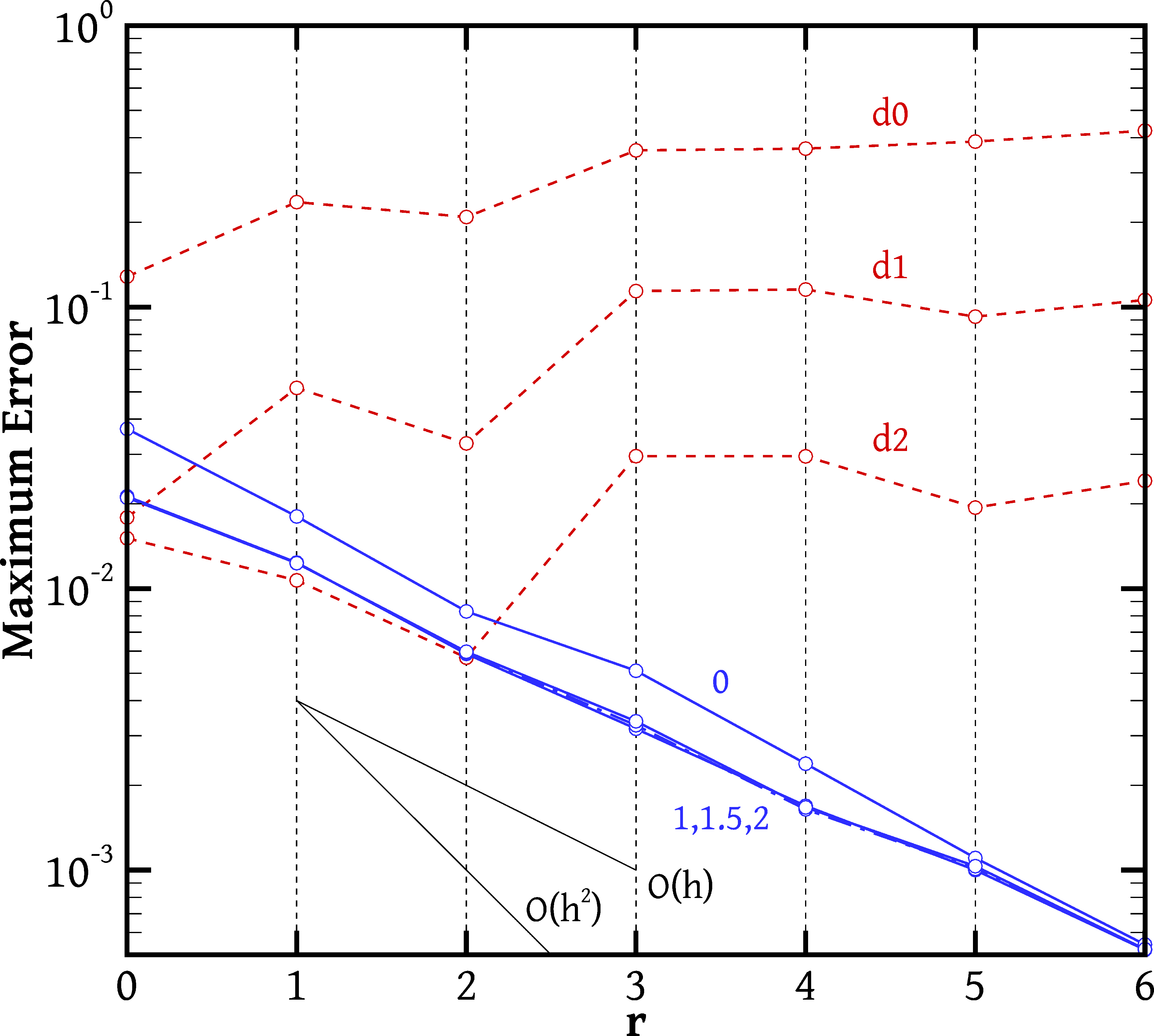
(b) maximum error, $\tau_{\mathrm{max}}$

Figure 17: The mean 17(a) and maximum 17(b) errors (defined by Eqs. (36) and (37), respectively) of the gradient calculation methods applied on the function $\phi=\tanh(x)\tanh(y)$ on the series of globally distorted grids (Fig. 16). The blue solid lines correspond to the least squares methods with weight exponents $q$ = 0, 1 and 2, which are indicated on each curve; the blue dash-dot line corresponds to the least squares method with $q=3/2$; and the red dashed lines correspond to the divergence theorem methods $\mathrm{d}c$ where $c$ is the number of corrector steps.

As far as the maximum errors are concerned, Fig. 17(b) shows that those of the LS methods decrease at a first order rate, with the unweighted method being the least accurate. On the other hand, the maximum errors of the DT methods actually increase with grid refinement. Presumably this is due to the fact that as the number of grid nodes is increased the probability of encountering higher degrees of skewness somewhere in the domain increases. Performing corrector steps reduces the error, but it is interesting to note that grid refinement causes a somewhat larger error increase when more corrector steps are performed. The deterioration of the $\nabla^{\mathrm{d}0}$ method with grid refinement propagates across the iterative correction procedure and eventually it is expected that the errors produced by the $\nabla^{\mathrm{d}c}$ operator used as a predictor will become so large that it will provide less (rather than more) accurate face centre values to the resulting “corrected” operator $\nabla^{\mathrm{d}(c+1)}$, making the latter worse than $\nabla^{\mathrm{d}c}$ itself.

Similarly to Sec. 5.3 we also tested the gradient schemes on a linear function. The results are listed in Table 3, together with grid quality metrics. Table 3 confirms that in the present case grid skewness and unevenness are roughly independent of grid refinement, i.e. their measures are $O(1)$, whereas they were $O(h)$ in the structured grid case (Table 1). As a result, the DT gradient schemes with a finite number of corrector steps ($\nabla^{\mathrm{d}0}$ and $\nabla^{\mathrm{d}1}$ in Table 3) now do not converge to the exact gradient. In the limit of infinite corrector steps the DT gradient ($\nabla^{\mathrm{d}\infty}$) becomes exact for linear functions, as are all the LS gradient schemes ($\nabla^{\mathrm{ls}0}$ and $\nabla^{\mathrm{ls}1}$ in Table 3).

Table 3: Mean errors (Eq. (36)) of various schemes for calculating the gradient $\nabla\phi=(1,2)$ of the linear function $\phi(x,y)=x+2y+0.5$ on the series of grids shown in Fig. 16. Also displayed are the measures of grid skewness and unevenness (defined in Sec. 2), averaged over all faces of each grid excluding boundary faces.

Grid $r$	Skew.	Unev.	$\nabla^{\mathrm{d}0}$	$\nabla^{\mathrm{d}1}$	$\nabla^{\mathrm{d}\infty}$	$\nabla^{\mathrm{ls}0}$	$\nabla^{\mathrm{ls}1}$
0	4.79$\cdot 10^{-2}$	4.94$\cdot 10^{-2}$	1.99$\cdot 10^{-1}$	1.55$\cdot 10^{-2}$	3.83$\cdot 10^{-15}$	9.84$\cdot 10^{-16}$	1.05$\cdot 10^{-15}$
1	5.46$\cdot 10^{-2}$	5.32$\cdot 10^{-2}$	2.43$\cdot 10^{-1}$	1.96$\cdot 10^{-2}$	7.29$\cdot 10^{-15}$	1.55$\cdot 10^{-15}$	1.59$\cdot 10^{-15}$
2	4.97$\cdot 10^{-2}$	5.14$\cdot 10^{-2}$	2.17$\cdot 10^{-1}$	1.61$\cdot 10^{-2}$	1.48$\cdot 10^{-14}$	3.07$\cdot 10^{-15}$	3.15$\cdot 10^{-15}$
3	5.16$\cdot 10^{-2}$	5.16$\cdot 10^{-2}$	2.29$\cdot 10^{-1}$	1.81$\cdot 10^{-2}$	2.94$\cdot 10^{-14}$	6.11$\cdot 10^{-15}$	6.18$\cdot 10^{-15}$
4	5.22$\cdot 10^{-2}$	5.17$\cdot 10^{-2}$	2.32$\cdot 10^{-1}$	1.89$\cdot 10^{-2}$	5.87$\cdot 10^{-14}$	1.22$\cdot 10^{-14}$	1.23$\cdot 10^{-14}$
5	5.18$\cdot 10^{-2}$	5.17$\cdot 10^{-2}$	2.32$\cdot 10^{-1}$	1.86$\cdot 10^{-2}$	1.18$\cdot 10^{-13}$	2.45$\cdot 10^{-14}$	2.45$\cdot 10^{-14}$
6	5.18$\cdot 10^{-2}$	5.14$\cdot 10^{-2}$	2.32$\cdot 10^{-1}$	1.87$\cdot 10^{-2}$	2.34$\cdot 10^{-13}$	4.86$\cdot 10^{-14}$	4.86$\cdot 10^{-14}$

6 Use of the gradient schemes within finite volume PDE solvers

So far we have examined the gradient schemes per se, examining their truncation error through mathematical tools and numerical experiments. Although there are examples of independent use of a gradient scheme such as in post-processing, the application of main interest is within finite volume methods (FVMs) for the solution of partial differential equations (PDEs). The gradient scheme is but a single component of the FVM and how it affects the overall accuracy depends also on the PDE solved as well as on the rest of the FVM discretisation. In the present section we provide some general comments and some simple demonstrations. The focus is on the effect of the gradient scheme on unstructured grids, where the DT scheme was shown to be inconsistent; on such grids the tests of Sec. 5.5 showed that the weights exponent of the LS method plays a minor role and so we only test the $q=1$ LS variant.

We begin with the observation that the approximation formula (10) is very similar to the formulae used by FVMs for integrating convective terms of transport equations over grid cells. Therefore, according to the same reasoning as in Section 3, such formulae also imply truncation errors of order $O(1)$ on arbitrary grids; this is true even if an interpolation scheme other than (9) is used to calculate $\bar{\phi}(\bm{c}^{\prime}_{f})$, or even if the exact values $\phi(\bm{c}^{\prime}_{f})$ are known and used. The order of the truncation error can be increased to $O(h)$ by accounting for skewness through a correction such as (16), provided that the gradient used is at least first-order accurate. These observations may raise concern about the overall accuracy of the FVM; however, it is known that the order of reduction of the discretisation error with grid refinement is often greater than that of the truncation error. Thus, $O(1)$ truncation errors do not necessarily imply $O(1)$ discretisation errors; the latter can be of order $O(h)$ or even $O(h^{2})$. This phenomenon has been observed by several authors (including the present ones [36]) and a literature review can be found in [39]. The question then naturally arises of whether and how the accuracy of the gradient scheme would affect the overall accuracy of the FVM that uses it. A general answer to this question does not yet exist, and each combination of PDE / discretisation scheme / grid type must be examined separately. For simple cases such as one-dimensional ones the problem can be tackled using theoretical tools but on general unstructured grids this has not yet been achieved [39]. Thus we will resort to some simple numerical experiments that amount to solving a Poisson equation.

6.1 Tests with an in-house solver

We solve the following Poisson equation:

$$\nabla\cdot\left(-k\nabla\phi\right)\;=\;b(x,y) \mathrm{on}\;\Omega=[0,1]\!\times\![0,1]$$ (42)

$$\phi\;=\;c(x,y) \mathrm{on}\;S_{\Omega}$$ (43)

with $k=1$, where $S_{\Omega}$ is the boundary of the domain $\Omega$ (the unit square), and

$$b(x,y)\; =\;2\tanh(x)\tanh(y)\left[2-(\tanh(x))^{2}-(\tanh(y))^{2}\right]$$ (44)

$$c(x,y)\; =\;\tanh(x)\tanh(y)$$ (45)

This is a heat conduction equation with a heat source term and Dirichlet boundary conditions. The source term was chosen such that the exact solution of the above equation is precisely $\phi=c(x,y)$. The domain was discretised by a series of progressively finer grids of $32\times 32$, $64\times 64$, …, $512\times 512$ cells denoted as grids 0, 1, …4, respectively. The grids were generated by the same randomised distortion procedure as those of Fig. 16, only that their boundaries are straight (Fig. 20). Corresponding undistorted Cartesian grids were also used for comparison. According to the FV methodology, we integrate Eq. (42) over each cell, apply the divergence theorem and use the midpoint integration rule to obtain for each cell $P$ a discrete equation of the following form:

$$\sum_{f=1}^{F}D_{f}\;=\;b(\bm{P})\,\Omega_{P}$$ (46)

where $b(\bm{P})$ is the value of the source term at the centre of cell $P$ and

$$D_{f}\;=\;\int_{S_{f}}-k\nabla\phi\cdot\bm{n}_{f}\,\mathrm{d}S\;\approx\;-S_{f}\,k\,\nabla\phi(\bm{c}_{f})\cdot\bm{n}_{f}$$ (47)

is the diffusive flux through face $f$ of the cell. We will test here two alternative discretisations of the fluxes $D_{f}$, both of which utilise some discrete gradient operator.

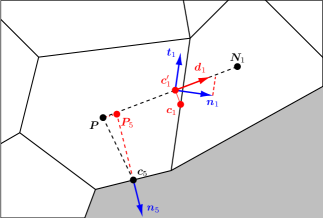
Figure 18: 18 Adopted notation for the “over-relaxed” diffusion scheme (Eq. (48)) and for the scheme for boundary faces (Eq. (50)); 18 Notation for the custom scheme (49). Face 1 of cell $P$ is an inner face, while its face 5 is a boundary face.

The first is the “over-relaxed” scheme [8, 40] which, according to [41], is very popular and is the method of choice in commercial and public-domain codes such as FLUENT, STAR-CD, STAR-CCM+ and OpenFOAM. This scheme splits the normal unit vector $\bm{n}_{f}$ in (47) into two components, one in the direction $\bm{N}_{f}-\bm{P}$ and one tangent to the face. The unit vectors along these two directions are denoted as $\bm{d}_{f}$ and $\bm{t}_{f}$, respectively (Fig. 18). Thus, if $\bm{n}_{f}=\alpha\bm{d}_{f}+\beta\bm{t}_{f}$ then by taking the dot product of this expression with $\bm{n}_{f}$ itself and noting that $\bm{t}_{f}$ and $\bm{n}_{f}$ are perpendicular ($\bm{n}_{f}\cdot\bm{t}_{f}=0$) we obtain $\alpha=(\bm{d}_{f}\cdot\bm{n}_{f})^{-1}$. We can therefore split $\bm{n}_{f}=\bm{d}_{f}^{*}+\bm{t}_{f}^{*}$ where $\bm{d}_{f}^{*}=\bm{d}_{f}/(\bm{d}_{f}\cdot\bm{n}_{f})$ and $\bm{t}_{f}^{*}=\beta\bm{t}_{f}$ calculated most easily as $\bm{t}_{f}^{*}=\bm{n}_{f}-\bm{d}_{f}^{*}$. Then the flux (47) is approximated as

$$D_{f}\; \approx\;-S_{f}\,k\,(\nabla\phi(\bm{c}^{\prime}_{f})\cdot\overbrace{\bm{d}_{f})\frac{1}{(\bm{n}_{f}\cdot\bm{d}_{f})}}^{\bm{d}_{f}^{*}}\;-\;S_{f}\,k\,\nabla\phi(\bm{c}^{\prime}_{f})\cdot\bm{t}_{f}^{*}$$

$$\approx\;-S_{f}\,k\,\frac{\phi(\bm{N}_{f})-\phi(\bm{P})}{\|\bm{N}_{f}-\bm{P}\|}\,\frac{1}{(\bm{d}_{f}\cdot\bm{n}_{f})}\;-\;S_{f}\,k\,\overline{\nabla^{\mathrm{a}}\phi}(\bm{c}^{\prime}_{f})\cdot\bm{t}_{f}^{*}$$

$$=\;-S_{f}\,k\,\frac{\phi(\bm{N}_{f})-\phi(\bm{P})}{(\bm{N}_{f}-\bm{P})\cdot\bm{n}_{f}}\;-\;S_{f}\,k\,\overline{\nabla^{\mathrm{a}}\phi}(\bm{c}^{\prime}_{f})\cdot\bm{t}_{f}^{*}$$ (48)

where $\nabla^{\mathrm{a}}$ is a discretised gradient calculated at the cell centres (either a DT gradient $\nabla^{\mathrm{d}}$ or the LS gradient $\nabla^{\mathrm{ls}}$) whose role we wish to investigate, and $\overline{\nabla^{\mathrm{a}}\phi}(\bm{c}^{\prime}_{f})$ is its value calculated at point $\bm{c}^{\prime}_{f}$ by linear interpolation (9). This scheme obviously deviates somewhat from the midpoint integration rule, substituting $\nabla\phi(\bm{c}^{\prime}_{f})\cdot\bm{n}_{f}$ instead of $\nabla\phi(\bm{c}_{f})\cdot\bm{n}_{f}$ in (47), i.e. it does not account for skewness.

We also try an alternative scheme which is the standard scheme in our code [42] and is a slight modification of a scheme proposed in [1]:

$$D_{f}\;\approx\;-S_{f}\,k\,\frac{\phi(\bm{N}^{\prime}_{f})-\phi(\bm{P}^{\prime})}{\|\bm{N}^{\prime}_{f}-\bm{P}^{\prime}\|}$$ (49)

where

$$\phi(\bm{P}^{\prime})\; \approx\;\phi(\bm{P})\;+\;\nabla^{\mathrm{a}}\phi(\bm{P})\cdot(\bm{P}^{\prime}-\bm{P})$$

$$\phi(\bm{N}^{\prime}_{f})\; \approx\;\phi(\bm{N}_{f})\;+\;\nabla^{\mathrm{a}}\phi(\bm{N}_{f})\cdot(\bm{N}^{\prime}_{f}-\bm{N}_{f})$$

and points $\bm{P}^{\prime}$ and $\bm{N}^{\prime}_{f}$ (Fig. 18) are such that the line segment joining these two points has length $\|\bm{N}_{f}-\bm{P}\|$, is perpendicular to face $f$, and its midpoint is $\bm{c}_{f}$. Thus this scheme tries to account for skewness. We will refer to this as the “custom” scheme.

Finally, irrespective of whether scheme (48) or (49) is used for the inner face fluxes, the boundary face fluxes are always calculated as

$$D_{f}\;\approx\;-S_{f}\,k\,\frac{\phi(\bm{c}_{f})-\phi(\bm{P}_{f})}{\|\bm{c}_{f}-\bm{P}_{f}\|}$$ (50)

where $f$ is a boundary face, point $\bm{P}_{f}$ is the projection of $\bm{P}$ on the line which is perpendicular to face $f$ and passes through $\bm{c}_{f}$ (see Fig. 18), and

$$\phi(\bm{P}_{f})\;\approx\;\phi(\bm{P})\;+\;\nabla^{\mathrm{a}}\phi(\bm{P})\cdot(\bm{P}_{f}-\bm{P})$$

Grid non-orthogonality activates in all schemes, (48), (49) and (50), a component that involves the approximate gradient $\nabla^{\mathrm{a}}$ (it is activated in (49) also by unevenness or skewness). It is not hard to show that this component contributes $O(1)$ to the truncation error if $\nabla^{\mathrm{a}}$ is first-order accurate, and $O(1/h)$ if it is zeroth-order accurate. On the undistorted Cartesian grids that were used for comparison the $\nabla^{\mathrm{a}}$ terms of the schemes are not activated; in fact, schemes (48) and (49) reduce to the same simple formula there. The reason why we do not simply substitute $\overline{\nabla^{\mathrm{a}}\phi}(\bm{c}_{f})$ for $\nabla\phi(\bm{c}_{f})$ in Eq. (47) instead of using schemes such as (48) and (49) is that this would allow spurious high-frequency (cell-to-cell) oscillations in the numerical solution $\phi$. This occurs because the $\nabla^{\mathrm{a}}$ calculation is mostly based on differences of $\phi$ values that are two cells apart, and so the gradient field $\nabla^{\mathrm{a}}\phi$ can be smooth even though $\phi$ oscillates from cell to cell. Schemes such as (48) and (49) express the diffusive flux mostly as a function of the direct difference of $\phi$ across the face, $\phi(\bm{N}_{f})-\phi(\bm{P})$, and thus do not allow such oscillations to go undetected. The gradients $\nabla^{\mathrm{a}}$ are used in an auxiliary fashion, in order to make the diffusive fluxes consistent. However, it has recently been shown [43, 44, 45] that schemes such as (48) and (49) can also be interpreted as equivalent to substituting an interpolated value of $\nabla^{\mathrm{a}}\phi$ for $\nabla\phi(\bm{c}_{f})$ in (47) and adding a damping term which is a function of the direct difference $\phi(\bm{N}_{f})-\phi(\bm{P})$ and of the gradients $\nabla^{\mathrm{a}}\phi(\bm{P})$ and $\nabla^{\mathrm{a}}\phi(\bm{N}_{f})$ and tends to zero with grid refinement.

Table 4: Number of outer iterations for convergence (residual per unit volume below $10^{-8}$) of the over-relaxed (48) and custom (49) schemes for solving the Poisson equation (42) – (45) on the $512\times 512$ distorted grids, employing various gradient schemes. Also shown is the percentage of CPU time spent on computing the gradient.

Scheme		$\nabla^{\mathrm{d}0}$	$\nabla^{\mathrm{d}1}$	$\nabla^{\mathrm{d}2}$	$\nabla^{\mathrm{d}\infty}$	$\nabla^{\mathrm{dx}}$	$\nabla^{\mathrm{ls}}$
Over-relaxed	iterations	901	617	601	786	573	585
	CPU %	6.8	14.9	22.1	9.7	17.2	14.3
Custom	iterations	792	874	914	752	919	919
	CPU %	7.4	16.5	23.6	10.5	17.9	15.2

The system of discrete equations (46) is linear, but for convenience it was solved with a fixed-point iteration procedure where in each outer iteration a linear system is solved (by a few inner iterations of a preconditioned conjugate gradient solver) whose equations involve only the unknowns at a cell and at its immediate neighbours, thus avoiding extended stencils. The matrix of this linear system is assembled only from the parts of Eq. (48) or (49) that directly involve $\phi(\bm{P})$ and $\phi(\bm{N}_{f})$, while the terms involving the gradients are calculated using the estimate of $\phi$ from the previous outer iteration and incorporated into the right-hand side of the linear system, as is customary. Outer iterations were carried out until the magnitude of the residual per unit volume had fallen below $10^{-8}$ in every grid cell, and the number of required such iterations for each diffusion flux scheme and gradient scheme are listed in Table 4, where the operator $\nabla^{\mathrm{d}\infty}$ is obtained with the scheme (22), while the operator $\nabla^{\mathrm{dx}}$ is the one obtained by applying the divergence theorem to the auxiliary cell of Fig. 6. Table 4 includes the percentage of the total calculation time consumed in calculating the gradient. It may be seen that the cost of corrector steps is quite significant, with the $\nabla^{\mathrm{d}2}$ gradient requiring more than 22% of the total computational effort. On the other hand, the scheme (22) is quite efficient, obtaining the $\nabla^{\mathrm{d}\infty}$ gradient at a cost that is almost as low as that of $\nabla^{\mathrm{d}0}$; however, in the case of the over-relaxed scheme, it also requires somewhat more outer iterations for convergence. The LS gradient costs about the same as the $\nabla^{\mathrm{d}1}$ gradient. The cost of the $\nabla^{\mathrm{dx}}$ gradient appears somewhat inflated due to a quick but not very efficient implementation. Overall, it seems that the iterative convergence rate depends mostly on the chosen flux discretisation scheme rather than on the choice of gradient scheme: in most cases the over-relaxed scheme converges faster than the custom scheme, which is not surprising since the former is known for its robustness [41]. Nevertheless, the choice of gradient scheme may significantly affect the iterative convergence rate in the FVM solution of other kinds of problems (depending of course also on the choice of FVM discretisation and iterative solver). In [26] it is reported that for convection problems unweighted LS gradients can result in much better iterative convergence than weighted ones, and that including more distant neighbours in the LS gradient computation also improves convergence.

The discretisation errors with respect to grid refinement are plotted in Fig. 19 for various flux and gradient scheme combinations. The discretisation error is defined as the difference between the exact solution $\phi$ of the problem (42) – (43) and the numerical (FVM) solution; Fig. 19(a) plots the mean absolute value of the discretisation error over all grid cells, and Fig. 19(b) plots the maximum absolute value.

(a) mean error, $\epsilon_{\mathrm{mean}}$

(b) maximum error, $\epsilon_{\mathrm{max}}$

Figure 19: The mean 19(a) and maximum 19(b) discretisation errors of various FVM schemes to solve the diffusion problem (42) – (45), on a series of highly distorted quadrilateral grids (Fig. 20). Grids 0, 1, …, 4 have $32\times 32$, $64\times 64$, …, $512\times 512$ volumes, respectively. DT0, DT1, DT2, DT, DTX and LS (solid lines) denote the “over-relaxed” scheme (48) with the $\nabla^{\mathrm{d}0}$, $\nabla^{\mathrm{d}1}$, $\nabla^{\mathrm{d}2}$, $\nabla^{\mathrm{d}\infty}$, $\nabla^{\mathrm{dx}}$ and $\nabla^{\mathrm{ls}}$ gradient schemes, respectively. DT1c, DTc, DTXc and LSc (dash-dot lines) denote the “custom” scheme (49) with the respective gradient schemes. C denotes results on Cartesian grids, where all methods are identical.

The first thing that one can notice from Figure 19 is that the common DT gradient ($\nabla^{\mathrm{d0}}$, $\nabla^{\mathrm{d1}}$, $\nabla^{\mathrm{d2}}$) leads to zeroth-order accuracy with respect to both the mean and maximum discretisation errors, irrespective of whether the over-relaxed or custom flux scheme is used. Similar trends as those of Fig. 17 are observed: corrector steps reduce the error but are eventually unable to converge to the exact solution. Although on coarse grids the DT1 and DT2 lines give the impression that they converge, eventually grid refinement cannot reduce the error below a certain point. In fact, an increase of the mean error can be observed on grid 4. Things are worse when the DT gradient is used in combination with the custom scheme (line DT1c), presumably because the gradient $\nabla^{\mathrm{a}}$ plays a more significant role in that scheme than in the over-relaxed scheme.

On the other hand, the $\nabla^{\mathrm{d\infty}}$ gradient obtained through the iterative procedure (22), the “auxiliary cell” gradient $\nabla^{\mathrm{dx}}$, and the LS gradient $\nabla^{\mathrm{ls}}$, all lead to second-order convergence to the exact solution. As long as the gradient scheme is consistent, the FVM accuracy seems to depend not on the gradient scheme but on the flux scheme, i.e. lines DT, LS and DTX (over-relaxed scheme (48)) nearly coincide, as do lines DTc, LSc and DTXc (custom scheme (49)). The mean discretisation error of the custom scheme is about the same as that obtained on Cartesian grids (line C), or even marginally lower when used in combination with the $\nabla^{\mathrm{d\infty}}$ gradient! The mean discretisation error of the over-relaxed scheme is only about 40% higher, which is a very good performance given that it does not account for skewness and that its iterative convergence is better (Table 4).

6.2 Tests with OpenFOAM

In order to investigate further the severity of the problem associated with the use of the common DT gradient we performed also a set of experiments using the popular public domain CFD solver OpenFOAM (https://openfoam.org), version 4.0, (see e.g. [46]) which we have been using recently in our laboratory [47, 48]. We solved again a Poisson problem (42) – (43) but instead of (45) and (44) we have $c(x,y)=\sin(\pi x)\sin(\pi y)$ and $b(x,y)=2\pi^{2}c(x,y)$, respectively. The problem was solved on the same set of grids composed of distorted quadrilaterals (Fig. 20), but, as these are artificially distorted grids, we also repeated the calculations using a couple of popular grid generation procedures which are more typical of real-life engineering applications, namely the Netgen [49] (https://ngsolve.org) and Gmsh Delaunay [50] (http://gmsh.info) algorithms implemented as plugins in the SALOME preprocessor (www.salome-platform.org). Both generate grids of triangular cells, coarse samples of which are shown in Fig. 20. The Netgen algorithm can be seen to be effective in producing smooth grid, reminiscent of that shown in Fig. 5, in four distinct areas within the domain that meet at an “X”-shaped interface where grid distortion is high. The Gmsh grids are less regular. The “LaplacianFoam” component of OpenFOAM was used to solve the equations with default options, which include the DT gradient (10) as the chosen gradient scheme (option “gradSchemes” is set to “Gauss linear”). We repeated the calculations with the gradient option set to LS (gradSchemes: leastSquares).

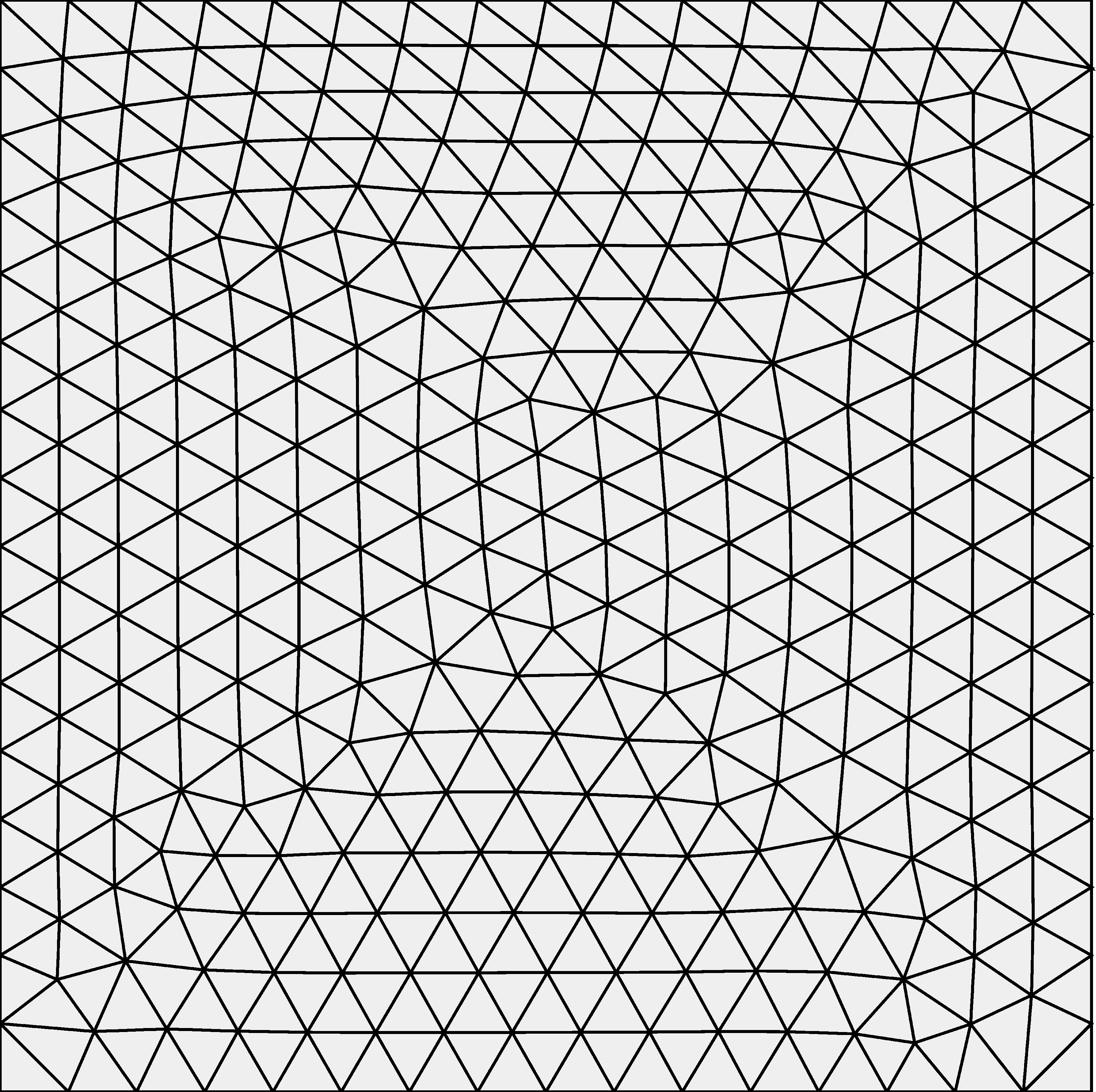
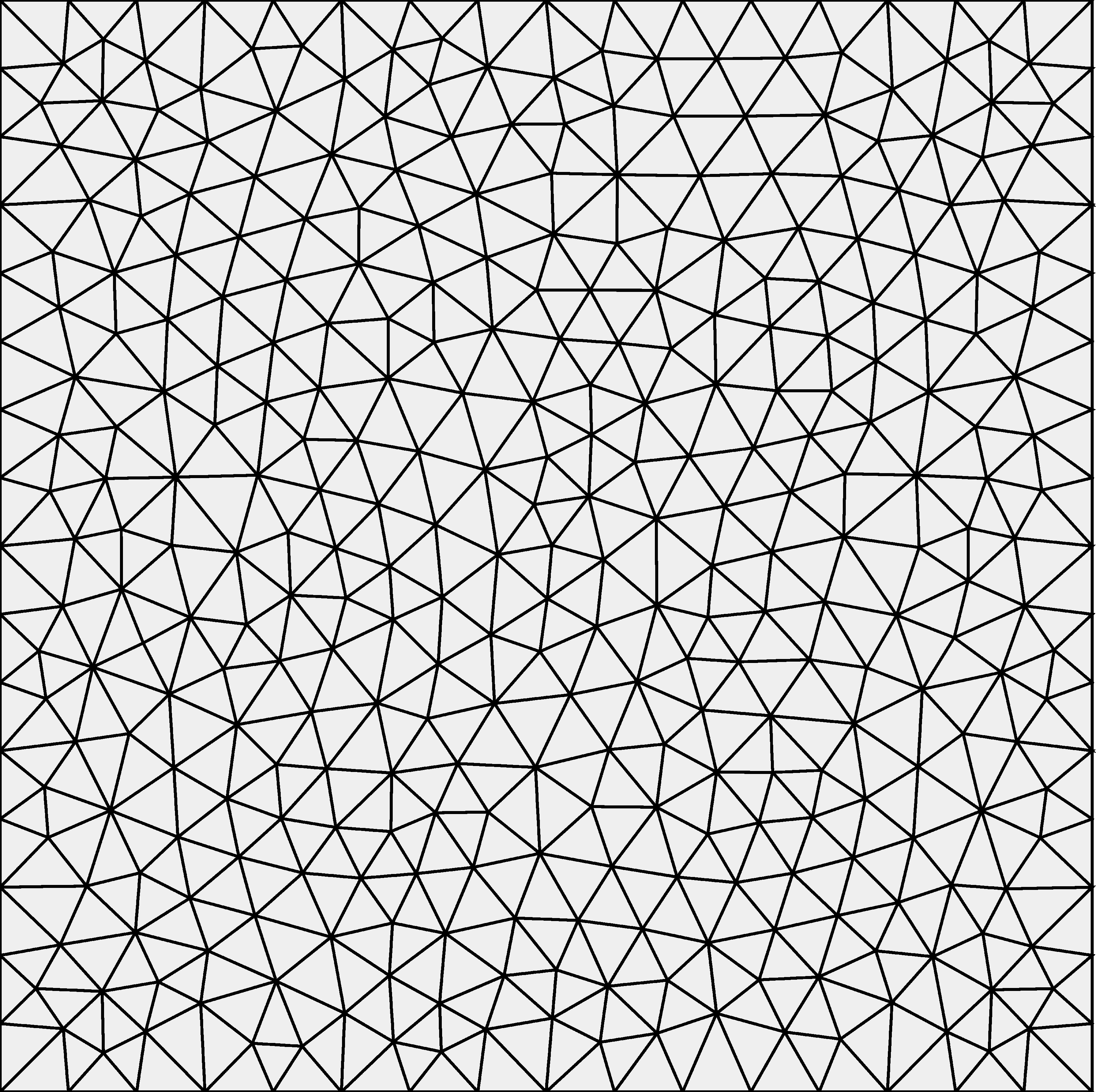
Figure 20: Samples from each grid category employed to solve the 2D Poisson problems using OpenFOAM: 20 a grid of distorted quadrilaterals; 20 a grid constructed with the Netgen algorithm; 20 a grid constructed with the Gmsh algorithm. All domains have unit length along each dimension.

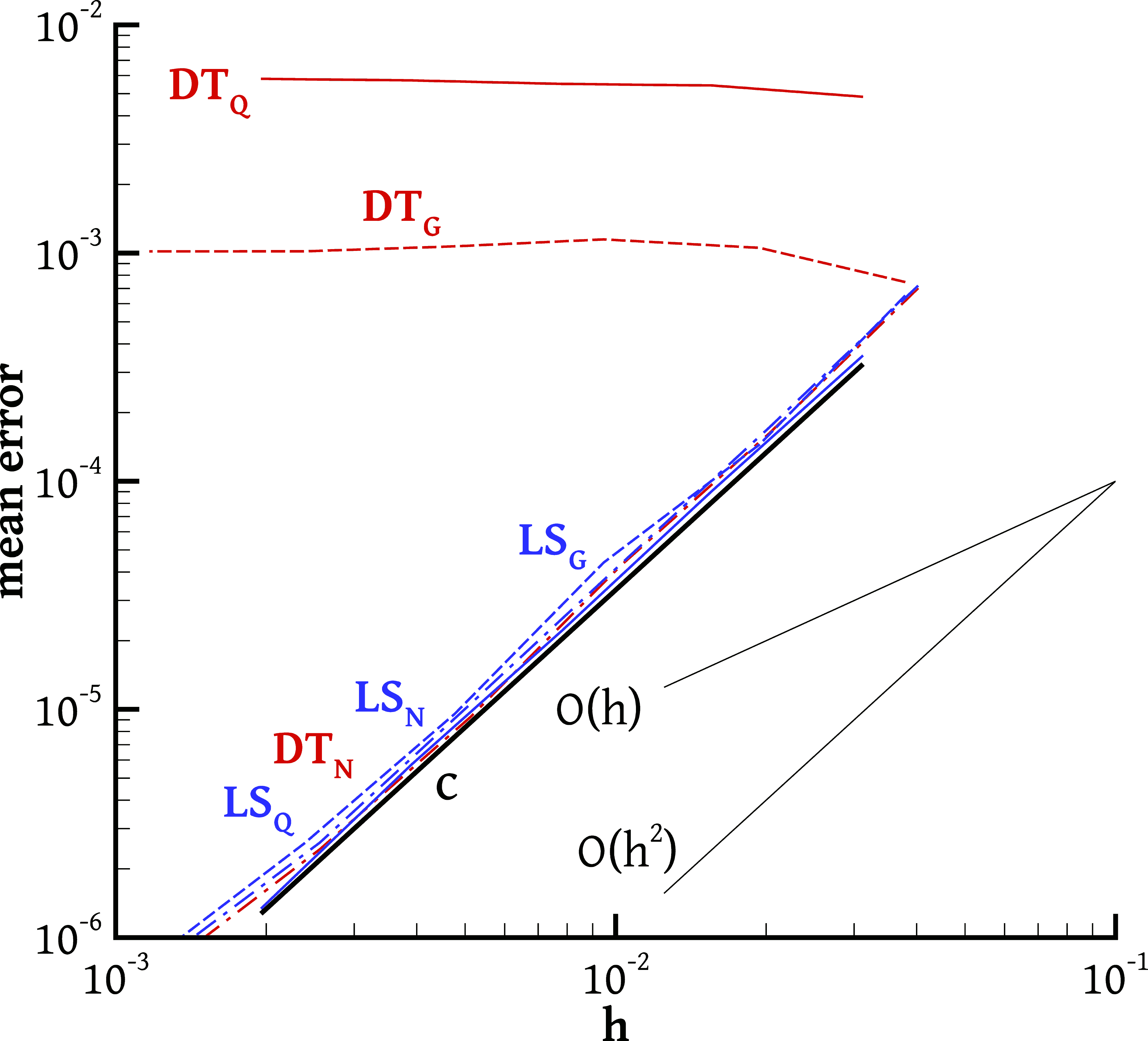
(a) mean error, 2D problem

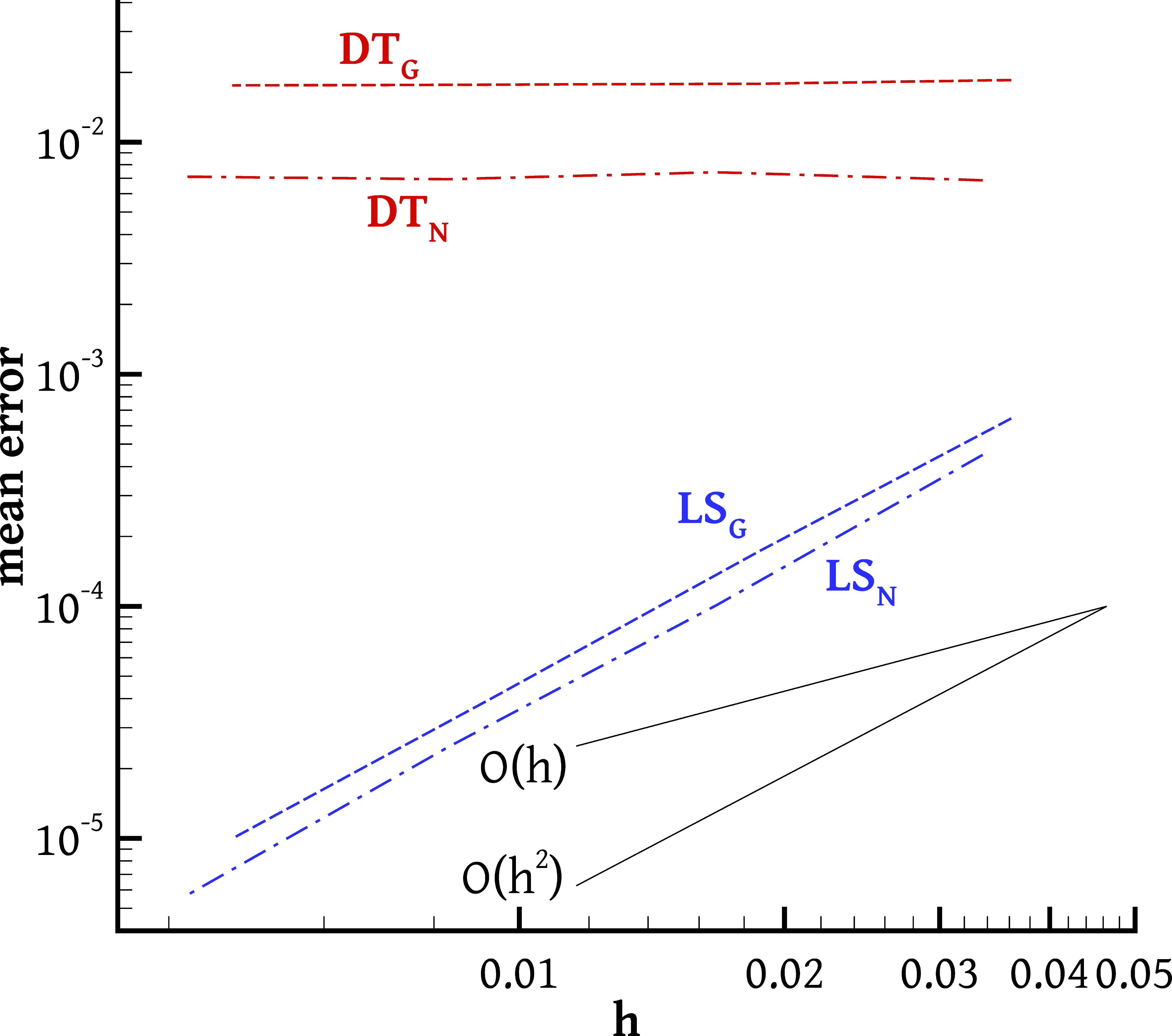
(b) mean error, 3D problem

Figure 21: The mean errors of the OpenFOAM solutions of the 2D 21(a) and 3D 21(b) Poisson equations, for various configurations. The abscissa $h$ is the mean cell size, $h=(\Omega/M)^{1/d}$ where $\Omega=1$ is the domain volume, $M$ is the total number of grid cells, and $d=2$ (for 2D) or $3$ (for 3D). The black solid line (C) corresponds to the 2D problem solved on undistorted Cartesian grids. Red lines (DT) and blue lines (LS) correspond to results obtained with the DT and LS gradients, respectively. Subscript Q ($\mathrm{DT}_{\mathrm{Q}}$, $\mathrm{LS}_{\mathrm{Q}}$ – solid lines) corresponds to grids of distorted quadrilaterals (Fig. 20). Subscript N ($\mathrm{DT}_{\mathrm{N}}$, $\mathrm{LS}_{\mathrm{N}}$ – dash-dot lines) corresponds to Netgen grids (Fig. 20). Subscript G ($\mathrm{DT}_{\mathrm{G}}$, $\mathrm{LS}_{\mathrm{G}}$ – dashed lines) corresponds to Gmsh Delaunay grids (Fig. 20).

The discretisation errors are plotted in Fig. 21(a), against the mean cell size $h$. We note that on the distorted quadrilateral grids and on the Gmsh grids the DT gradient (lines $\mathrm{DT}_{\mathrm{Q}}$ and $\mathrm{DT}_{\mathrm{G}}$) engenders zeroth-order accuracy, like the DT0 case of Fig. 19. On the other hand, the Netgen grids are quite smooth (Fig. 20), resembling grids that come from triangulation of structured grids in most of the domain, and this has the consequence that even with the DT gradient (lines $\mathrm{DT}_{\mathrm{N}}$) the mean error decreases at a second-order rate. With the LS gradient second-order accuracy is exhibited on all grids, and furthermore the accuracy is nearly at the same level as on the Cartesian grids.

Three-dimensional simulations were also performed. The governing equations are again (42) – (43) where we set $c(x,y,z)=\sin(\pi x)\sin(\pi y)\sin(\pi z)$ and $b(x,y,z)=3\pi^{2}c(x,y,z)$. The domain is the unit cube $z,y,z\in[0,1]$ and the grids were generated with the Netgen and Gmsh algorithms, where in the latter we chose the Delaunay method to construct the grid at the boundaries and the frontal Delaunay algorithm to construct the grid in the interior. The discretisation errors are plotted in Fig. 21(b). This time it is observed that the DT gradient engenders zeroth-order accuracy even on the Netgen grids. Presumably, in the 3D case although the Netgen algorithm produces relatively smooth surface grids on the bounding surfaces of the cube, in the bulk of the domain it packs the tetrahedra in a way that the skewness is large throughout. On the other hand, the LS gradient again always results in second-order accuracy.

7 Final remarks and conclusions

The previous sections showed that on arbitrary grids the DT and LS gradients are zeroth- and first-order accurate, respectively, but higher orders of accuracy, up to second, are obtained on particular kinds of grids – a summary of the present findings is given in Table 5.

Unfortunately, general-purpose unstructured grid generation algorithms, such as the popular Netgen and Gmsh algorithms tested in Sec. 6, retain high skewness at all levels of refinement (except in the 2D Netgen case) resulting in zeroth-order accuracy for both the DT gradient and the FVM solver that employs it. In our tests, OpenFOAM using the DT gradient was unable to reduce the discretisation errors by grid refinement even though the problems solved were very fundamental, namely linear Poisson problems with sinusoidal solutions on the simplest possible domains, the unit square and cube. Zeroth-order accuracy is very undesirable because it deprives the modeller of his/her main tool for estimating the accuracy of the solution, i.e. the grid convergence study. Therefore the common DT gradient should be avoided unless the grid refinement algorithm is known to reduce the skewness towards zero. This is especially important nowadays that automatic unstructured grid generation algorithms are preferred over structured grids. On the other hand, if the LS gradient is employed instead then the FVM for the problems of Sec. 6 proved to be second-order accurate on all grids, irrespective of whether their skewness diminishes or not with refinement. The same holds for consistent DT gradient schemes, such as the proposed iterative scheme (22), the scheme employing the auxiliary cell of Fig. 6, or any other consistent scheme mentioned in Sec. 3.

Table 5: Order of the mean and maximum truncation errors of the gradient schemes on various grid types.

	Common DT		LS $q\neq 3/2$,		LS $q=3/2$
			$\nabla^{\mathrm{d\infty}}$, $\nabla^{\mathrm{dx}}$
	mean	max.	mean	max.	mean	max.
Cartesian (§5.2)	2	1	2	1	2	2
Smooth Structured (§5.3)	2	1	2	1	2	2
Locally Distorted (§5.4)	1	0	2	1	2	1
Arbitrary (§5.5)	0	0	1	1	1	1

On grids where both methods exhibit the same order of accuracy the optimal method is problem-dependent. Usually schemes of the same order of accuracy will produce comparable errors on any given grid but in some cases the errors can differ significantly. For example, in aerodynamics problems concerning the boundary layer flow over a curved solid boundary, when structured grids consisting of cells of very high aspect ratio are employed the DT method is known to significantly outperform the LS method [16, 20] despite both being second-order accurate (or first-order, on triangulated grids). This is because the DT method benefits from the alignment of the cell faces with the flow (see Appendix C).

The present study has been restricted to the FVM solution of a Poisson problem. The effect of the choice of gradient discretisation scheme for the FVM solution of flow problems, including non-Newtonian or turbulent ones where the role of the gradient is more significant, will be investigated in a future study.

Appendix A Accuracy of the least squares gradient when the neighbouring points are arranged at equal angles

Consider the case that all angles between two successive neighbours are equal; this means that they are equal to $2\pi/F$ ($F$ being the total number of neighbours). Therefore,

$$\theta_{f}\;=\;\theta_{1}\;+\;(f-1)\,\frac{2\pi}{F}$$ (A.1)

As per Eq. (35), we will express $\beta_{\varsigma}$ in the error expression (31) substituting for $\varsigma_{f}$ from Eq. (25). We also substitute $\Delta x_{f}=\Delta r_{f}\cos\theta_{f}$ and $\Delta y_{f}=\Delta r_{f}\sin\theta_{f}$. In the special case that all neighbours are equidistant from $\bm{P}$, i.e. all $\Delta r_{f}$’s are equal, the weights $w_{f}$ are also equal and the products $(\Delta r_{f})^{3}w_{f}^{2}$ can be factored out of the sums:

$$\beta_{\tau}\;=\;(\Delta r_{f})^{3}w_{f}^{2}\begin{bmatrix}\frac{1}{2}\phi_{\!.xx}\sum\limits_{f=1}^{F}(\cos\theta_{f})^{3}\;+\;\phi_{\!.xy}\sum\limits_{f=1}^{F}(\cos\theta_{f})^{2}\sin\theta_{f}\;+\;\frac{1}{2}\phi_{\!.yy}\sum\limits_{f=1}^{F}\cos\theta_{f}(\sin\theta_{f})^{2}\\[11.38092pt] \frac{1}{2}\phi_{\!.xx}\sum\limits_{f=1}^{F}(\cos\theta_{f})^{2}\sin\theta_{f}\;+\;\phi_{\!.xy}\sum\limits_{f=1}^{F}\cos\theta_{f}(\sin\theta_{f})^{2}\;+\;\frac{1}{2}\phi_{\!.yy}\sum\limits_{f=1}^{F}(\sin\theta_{f})^{3}\end{bmatrix}$$ (A.2)

where higher-order terms are omitted. If the neighbours are not equidistant but the weight scheme $w_{f}=(\Delta r_{f})^{-3/2}$ is used, then all products $(\Delta r_{f})^{3}w_{f}^{2}=1$ are again equal and (A.2) still holds.

To proceed further, it will be convenient to use complex arithmetic: $\cos\theta_{f}=(e^{i\theta_{f}}+e^{-i\theta_{f}})/2$ and $\sin\theta_{f}=(e^{i\theta_{f}}-e^{-i\theta_{f}})/2i$, where $i\equiv\sqrt{-1}$. Then it is straightforward to show that the sums that appear in the right hand side of Eq. (A.2) are equal to

$$\sum\limits_{f=1}^{F}(\cos\theta_{f})^{3}\; =\;\frac{1}{8}\sum\limits_{f=1}^{F}\left(e^{i3\theta_{f}}\;+\;3e^{i\theta_{f}}\;+\;3e^{-i\theta_{f}}\;+\;e^{-i3\theta_{f}}\right)$$ (A.3)

$$\sum\limits_{f=1}^{F}(\cos\theta_{f})^{2}\sin\theta_{f}\; =\;\frac{1}{8i}\sum\limits_{f=1}^{F}\left(e^{i3\theta_{f}}\;+\;e^{i\theta_{f}}\;-\;e^{-i\theta_{f}}\;-\;e^{-i3\theta_{f}}\right)$$ (A.4)

$$\sum\limits_{f=1}^{F}\cos\theta_{f}(\sin\theta_{f})^{2}\; =\;-\frac{1}{8}\sum\limits_{f=1}^{F}\left(e^{i3\theta_{f}}\;-\;e^{i\theta_{f}}\;-\;e^{-i\theta_{f}}\;+\;e^{-i3\theta_{f}}\right)$$ (A.5)

$$\sum\limits_{f=1}^{F}(\sin\theta_{f})^{3}\; =\;-\frac{1}{8i}\sum\limits_{f=1}^{F}\left(e^{i3\theta_{f}}\;-\;3e^{i\theta_{f}}\;+\;3e^{-i\theta_{f}}\;-\;e^{-i3\theta_{f}}\right)$$ (A.6)

The above expressions involve the sums $\sum e^{i\theta_{f}}$, $\sum e^{-i\theta_{f}}$, $\sum e^{i3\theta_{f}}$ and $\sum e^{-i3\theta_{f}}$; if these sums are zero then the sums on the left hand sides of (A.3) – (A.6) are also zero and it follows, in the same way as for Eq. (35), that the LS gradient is second-order accurate. So, we consider the first of these sums, substituting for $\theta_{f}$ from Eq. (A.1).

$$\sum\limits_{f=1}^{F}e^{i\theta_{f}}\;=\;\sum\limits_{f=1}^{F}e^{i\left(\theta_{1}+(f-1)\frac{2\pi}{F}\right)}\;=\;e^{i\theta_{1}}\sum\limits_{f=1}^{F}e^{i(f-1)\frac{2\pi}{F}}$$ (A.7)

We denote $\zeta=e^{i2\pi/F}$ and note that it is the first $F$-th root of unity, i.e. $\zeta^{F}=e^{i2\pi F/F}=e^{i2\pi}=1$. Then the sum that appears at the end of Eq. (A.7) is

$$\sum\limits_{n=0}^{F-1}\zeta^{n}\;=\;1\;+\;\zeta\;+\;\zeta^{2}\;+\;\cdots\;+\;\zeta^{F-1}\;=\;0$$ (A.8)

Equation (A.8) holds for any $F$-th root of unity except $\zeta=1$, as follows from the identity $1-\zeta^{F}=(1-\zeta)(1+\zeta+\zeta^{2}+\cdots+\zeta^{F-1})$: the left hand side is zero because $\zeta^{F}=1$, so the right hand side must be zero as well, and since $\zeta\neq 1$, it follows that $(1+\zeta+\zeta^{2}+\cdots+\zeta^{F-1})=0$, i.e. Eq. (A.8) [28]. Thus $\sum e^{i\theta_{f}}=0$. In exactly the same manner it can be shown that $\sum e^{-i\theta_{f}}=0$ as well.

We proceed in the same way for the sum $\sum e^{i3\theta_{f}}$:

$$\sum\limits_{f=1}^{F}e^{i3\theta_{f}}\;=\;\sum\limits_{f=1}^{F}e^{i3\left(\theta_{1}+(f-1)\frac{2\pi}{F}\right)}\;=\;e^{i3\theta_{1}}\sum\limits_{f=1}^{F}e^{i3(f-1)\frac{2\pi}{F}}$$ (A.9)

This time we denote $\zeta=e^{i3(2\pi)/F}$. It is also an $F$-th root of unity, since $\zeta^{F}=e^{i3(2\pi)F/F}=e^{i6\pi}=1$. So, it will also satisfy Eq. (A.8), unless $\zeta=1$. Now, $\zeta=e^{i2\pi(3/F)}$ will be $\neq 1$ precisely if $3/F$ is not an integer, i.e. if $F$ is neither $1$ nor $3$. Thus, for $F\neq 3$ Eq. (A.8) still holds, and Eq. (A.9) says that $\sum e^{i3\theta_{f}}$ is zero. But if $F=3$ then $\sum e^{i3\theta_{f}}$ is not zero. The same holds for the last sum, $\sum e^{-i3\theta_{f}}$, as can be shown in exactly the same way.

So, to summarise, if $F>3$ then all the terms in (A.3) – (A.6) become zero and the leading term of the truncation error vanishes, granting second-order accuracy to the LS gradient, provided that the $q=3/2$ weights scheme is used (or that the neighbouring points are equidistant from $\bm{P}$). But if $F=3$ then not all terms vanish and the leading part of the truncation error does not reduce to zero – the gradient remains first-order accurate. This is unfortunate, as the $F=3$ case is very common, corresponding to triangular cells.

Appendix B Using a LS weights matrix with off-diagonal elements

Consider the one-dimensional case. For a general matrix $W$ the weighted LS method returns the value of $\phi_{\!.x}^{\mathrm{ls}}(\bm{P})$ which minimises the quantity

$$\|W(b-Az)\|^{2}\;=\;\sum_{i}\left[\sum_{j=1}^{F}w_{ij}\left(\Delta\phi_{j}-\Delta x_{j}\,\phi_{\!.x}^{\mathrm{ls}}(\bm{P})\right)\right]^{2}$$ (B.1)

It can be shown that if the method returns the exact derivative of any quadratic function $\phi$ then it is second-order accurate. The Taylor expansion of a quadratic function $\phi$ is just

$$\Delta\phi_{f}\;=\;\phi_{\!.x}(\bm{P})\,\Delta x_{f}\;+\;\frac{1}{2}\phi_{\!.xx}(\bm{P})\,(\Delta x_{f})^{2}$$ (B.2)

We can use this equation to substitute for $\Delta\phi_{j}$ into Eq. (B.1) to get

$$\|W(b-Az)\|^{2}\;=\;\sum_{i}\left[\left(\phi_{\!.x}(\bm{P})-\phi_{\!.x}^{\mathrm{ls}}(\bm{P})\right)\sum_{j=1}^{F}w_{ij}\Delta x_{j}\;+\;\frac{1}{2}\phi_{\!.xx}(\bm{P})\sum_{j=1}^{F}w_{ij}(\Delta x_{j})^{2}\right]^{2}$$

Apparently, if we can choose the weights so that $\sum_{j}w_{ij}(\Delta x_{j})^{2}=0$ for each row $i$ of $W$, then the terms involving $\phi_{\!.xx}(\bm{P})$ will vanish and the remaining quantity will be minimised (actually, made zero) by the choice $\phi_{\!.x}^{\mathrm{ls}}(\bm{P})=\phi_{\!.x}(\bm{P})$. Thus the procedure will produce the exact result. The equation $\sum_{j}w_{ij}(\Delta x_{j})^{2}=0$ can be written in matrix notation as $X\,w_{i}=0$, where $X$ is the $1\times F$ matrix with elements $X_{1j}=(\Delta x_{j})^{2}$ and $w_{i}$ is the $F\times 1$ column vector with elements $w_{ij}$. We can therefore set each row $w_{i}$ of $W$ equal to a basis vector of the null space of $X$. A simple choice is one where in row $f$ the first element is $(\Delta x_{1})^{-2}$, the $f\!+\!1$ element is $-(\Delta x_{f+1})^{-2}$, and the rest of the elements are zero. $W$ is no longer square but has size $(F\!-\!1)\times F$, so the weighted system $WAz=Wb$ has one less equation than the original system $Az=b$. Equation $i$ of the system $WAz=Wb$ has the form

$$\phi_{\!.x}^{\mathrm{ls}}(\bm{P})\,\left(\frac{1}{\Delta x_{i+1}}-\frac{1}{\Delta x_{1}}\right)\;=\;\frac{\Delta\phi_{i+1}}{(\Delta x_{i+1})^{2}}\;-\;\frac{\Delta\phi_{1}}{(\Delta x_{1})^{2}}$$ (B.3)

for $i=1,\ldots,F-1$. A little manipulation shows that Eq. (B.3) is just Eq. (B.2) for $f=i+1$, where $\phi_{\!.xx}(\bm{P})$ has been eliminated by using again Eq. (B.2), but for $f=1$, to express it as a function of $\Delta\phi_{1}$ and $\Delta x_{1}$. Therefore, this method is nearly equivalent to the unweighted LS solution of the system of equations (B.2). Extension to the 2D or 3D cases follows the same lines.

Appendix C The gradient schemes in aerodynamics problems

It is known in aerodynamics that the DT gradient is more accurate than the LS gradient for the computation of boundary layer flow over a curved solid boundary when grid cells of very high aspect ratio are employed (typically in excess of 1000) [16, 20]. This is due to a fundamental difference between the methods: the LS gradient uses the directions in which the neighbours lie, represented by the unit vectors $\bm{d}_{f}=(\bm{N}_{f}-\bm{P})/\|\bm{N}_{f}-\bm{P}\|$, while the DT gradient uses the directions normal to the faces, represented by the unit vectors $\bm{n}_{f}$. This allows the possibility of assisting the DT gradient by aligning the cell faces with the direction of the exact gradient, when this direction is known a priori.

So, consider a structured grid of high aspect ratio cells over a curved boundary as in Fig. 22 and assume a boundary layer flow where the contours of the dependent variable $\phi$ follow the shape of the boundary so that $\phi(\bm{P})=\phi(\bm{N}_{1})=\phi(\bm{N}_{3})\Rightarrow\Delta\phi_{1}=\Delta\phi_{3}=0$ and the exact $\nabla\phi$ is directed normal to the boundary with approximate magnitude $(\phi(\bm{N}_{2})-\phi(\bm{N}_{4}))/2\Delta y$. The grid being structured all of the examined methods are second order accurate, but the unweighted LS gradient is known to perform very poorly: From expression (32) it follows that because $\Delta r_{1}$ and $\Delta r_{3}$ are much larger than $\Delta r_{2}$ and $\Delta r_{4}$ this scheme relies on information mostly in the directions $\bm{d}_{1}$ and $\bm{d}_{3}$, and since the directional derivatives $\Delta\phi_{1}/\Delta r_{1}$ and $\Delta\phi_{3}/\Delta r_{3}$ in these directions appear to be zero, the predicted gradient is also near zero although the true gradient may be very large. This gross underestimation is known to occur when the ratio of $y$-displacements $\gamma/\Delta y$ of neighbours $N_{1}$ and $N_{3}$ to neighbours $N_{2}$ and $N_{4}$ (Fig. 22) is larger than one (i.e. when the terms $(\partial\phi/\partial y)^{\mathrm{ls}}\gamma$ are larger than the terms $(\partial\phi/\partial y)^{\mathrm{ls}}\Delta y$ in the minimisation expression), and in practical applications it is typically around 50 [16]. As this ratio is proportional to $(\Delta x)^{2}/(R\,\Delta y)$ [16], reducing the size $\Delta x$ of the cells in the streamwise direction rapidly reduces the error. Using a weighted LS method dramatically improves the accuracy, but this remedy does not work if the grid is triangulated as in Fig. 5.

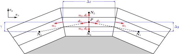
Figure 22: Structured grid of high aspect ratio cells over a curved boundary (the aspect ratio $\Delta x/\Delta y$ is greatly downplayed for clarity).

The inaccuracy of the LS gradients in this case is due to the invalidation of their fundamental assumption that the variation of $\phi$ in the neighbourhood of the cell is linear, as the cell size is large enough for the contours of $\phi$ to curve significantly across it. On the other hand, the DT gradient benefits from the alignment of the normals $\bm{n}_{2}$ and $\bm{n}_{4}$ of the long faces (which dominate the calculation due to weighting by face area) with the direction of the exact gradient. Thus, for this particular $\phi$ distribution the given grid alignment assists this gradient scheme to achieve good accuracy. A similar (somewhat less favourable) situation holds in the triangulated grid case.

Another issue is related to numerical stability. Certain discretisation schemes use the values of the dependent variable at face centres, evaluated as $\phi(\bm{c}_{f})\approx\phi(\bm{P})+\nabla^{\mathrm{a}}\phi(\bm{P})\cdot(\bm{c}-\bm{P})$. Consider the same boundary layer flow as before, but for the moment assume a straight boundary so that the grid looks like that of Fig. 2, on which all the examined gradient schemes reduce to $\nabla^{\mathrm{s}}$, Eq. (1). Since $\phi(\bm{N}_{1})=\phi(\bm{N}_{3})=\phi(\bm{P})$, Eq. (1) returns a gradient in the direction $(-\delta_{y}^{\xi},\delta_{x}^{\xi})$ i.e. perpendicular to the vector $\bm{\delta}^{\xi}$. Thus $\phi(\bm{c}_{1})\approx\phi(\bm{P})+\nabla^{\mathrm{s}}\phi(\bm{P})\cdot(\bm{c}_{1}-\bm{P})=\phi(\bm{P})=\phi(\bm{N}_{1})$, which is reasonable. Now consider a curved boundary case where cell $P$ has exactly the same shape as before but its neighbours $N_{1}$ and $N_{3}$ are tilted to follow the curvature as in Fig. 22. The DT gradient depends only on the face normals $\bm{n}_{f}$ which have not changed for cell $P$ and thus it gives the same result for $\phi(\bm{c}_{1})$ as before. On the other hand, the vectors $\bm{d}_{1}$ and $\bm{d}_{3}$ have now changed and thus the LS gradient is affected by the curvature and may no longer be perpendicular to the direction $\bm{c}_{1}-\bm{P}$; this leads to a predicted value for $\phi(\bm{c}_{1})$ that is either larger or smaller than both $\phi(\bm{P})$ and $\phi(\bm{N}_{1})$, introducing an oscillatory variation in the direction $\bm{d}_{1}$ that may be detrimental to numerical stability [18]. In other cases this issue can occur with both the LS and the DT gradients, and so some solvers such as OpenFOAM offer versions of these gradient schemes that use limiters in order to avoid this problem.

References

- [1] J. H. Ferziger and M. Peric, Computational methods for fluid dynamics. Springer, 3rd ed., 2002.
- [2] P. J. Oliveira, F. T. Pinho, and G. A. Pinto, “Numerical simulation of non-linear elastic flows with a general collocated finite-volume method,” J. Non-Newtonian Fluid Mech., vol. 79, pp. 1–43, 1998.
- [3] A. M. Afonso, M. S. N. Oliveira, P. J. Oliveira, M. A. Alves, and F. T. Pinho, “The finite volume method in computational rheology,” in Finite-Volume Methods – Powerful Means of Engineering Design, ch. 7, pp. 141–170, In-Tech Open Publishers, 2012.
- [4] A. Syrakos, G. Georgiou, and A. Alexandrou, “Solution of the square lid-driven cavity flow of a Bingham plastic using the finite volume method,” J. Non-Newtonian Fluid Mech., vol. 195, pp. 19–31, 2013.
- [5] A. Jalali, M. Sharbatdar, and C. Ollivier-Gooch, “An efficient implicit unstructured finite volume solver for generalised Newtonian fluids,” International Journal of Computational Fluid Dynamics, vol. 30, no. 3, pp. 201–217, 2016.
- [6] C. D. Correa, R. Hero, and K.-L. Ma, “A comparison of gradient estimation methods for volume rendering on unstructured meshes,” IEEE Trans. Visual Comput. Graphics, vol. 17, pp. 305–319, 2011.
- [7] T. J. Barth and D. C. Jespersen, “The design and application of upwind schemes on unstructured meshes,” in AIAA Paper 89-0366, 1989.
- [8] H. Jasak, Error Analysis and Estimation for the Finite Volume Method with Application to Fluid Flows. PhD thesis, Imperial College, London, 1996.
- [9] Ž. Lilek, S. Muzaferija, M. Perić, and V. Seidl, “An implicit finite-volume method using nonmatching blocks of structured grid,” Numer. Heat Transfer, vol. 32, pp. 385–401, 1997.
- [10] J. Wu and P. Traoré, “Similarity and comparison of three finite-volume methods for diffusive fluxes computation on nonorthogonal meshes,” Numer. Heat Transfer B, vol. 64, pp. 118–146, 2014.
- [11] F. Moukalled, L. Mangani, and M. Darwish, The Finite Volume Method in Computational Fluid Dynamics. Springer, 2016.
- [12] T. J. Barth, “A 3-D upwind Euler solver for unstructured meshes,” in AIAA Paper 91-1548-CP, 1991.
- [13] S. Muzaferija and D. A. Gosman, “Finite-volume CFD procedure and adaptive error control strategy for grids of arbitrary topology,” J. Comput. Phys., vol. 138, pp. 766–787, 1997.
- [14] C. Ollivier-Gooch and M. Van Altena, “A high-order-accurate unstructured mesh finite-volume scheme for the advection–diffusion equation,” J. Comput. Phys., vol. 181, pp. 729–752, 2002.
- [15] F. Bramkamp, P. Lamby, and S. Müller, “An adaptive multiscale finite volume solver for unsteady and steady state flow computations,” J. Comput. Phys., vol. 197, pp. 460–490, 2004.
- [16] D. J. Mavriplis, “Revisiting the least-squares procedure for gradient reconstruction on unstructured meshes,” in AIAA Paper 2003-3986, 2003.
- [17] B. Diskin and J. L. Thomas, “Accuracy of gradient reconstruction on grids with high aspect ratio,” tech. rep., NIA Report No. 2008-12, 2008.
- [18] E. Shima, K. Kitamura, and K. Fujimoto, “New gradient calculation method for MUSCL type CFD schemes in arbitrary polyhedra,” in AIAA Paper 2010-1081, 2010.
- [19] L. J. Betchen and A. G. Straatman, “An accurate gradient and Hessian reconstruction method for cell-centered finite volume discretizations on general unstructured grids,” Int. J. Numer. Methods Fluids, vol. 62, pp. 945–962, 2010.
- [20] E. Sozer, C. Brehm, and C. C. Kiris, “Gradient calculation methods on arbitrary polyhedral unstructured meshes for cell-centered CFD solvers,” in AIAA Paper 2014-1440, 2014.
- [21] A. Syrakos, Analysis of a finite volume method for the incompressible Navier-Stokes equations. PhD thesis, Aristotle University of Thessaloniki, 2006.
- [22] M. S. Karimian and A. G. Straatman, “Discretization and parallel performance of an unstructured finite volume Navier–Stokes solver,” Int. J. Numer. Methods Fluids, vol. 52, pp. 591–615, 2006.
- [23] Y. Kallinderis and C. Kontzialis, “A priori mesh quality estimation via direct relation between truncation error and mesh distortion,” J. Comput. Phys., vol. 228, pp. 881–902, 2009.
- [24] R. L. Burden and J. D. Faires, Numerical Analysis. Brooks/Cole, 9th ed., 2011.
- [25] Q. Wang, Y.-X. Ren, J. Pan, and W. Li, “Compact high order finite volume method on unstructured grids III: Variational reconstruction,” Journal of Computational Physics, vol. 337, pp. 1–26, may 2017.
- [26] B. Diskin and J. L. Thomas, “Comparison of node-centered and cell-centered unstructured finite-volume discretizations: Inviscid fluxes,” AIAA Journal, vol. 49, pp. 836–854, apr 2011.
- [27] L. N. Trefethen and D. Bau III, Numerical Linear Algebra. SIAM, 1997.
- [28] G. Strang, Linear Algebra and its Applications. Brooks/Cole, 4th ed., 2006.
- [29] S. Muzaferija, Adaptive Finite Volume Method for Flow Prediction using Unstructured Meshes and Multigrid Approach. PhD thesis, Imperial College, London, 1994.
- [30] Y. Liu and W. Zhang, “Accuracy preserving limiter for the high-order finite volume method on unstructured grids,” Computers & Fluids, vol. 149, pp. 88–99, 2017.
- [31] J.-M. Vaassen, D. Vigneron, and J.-A. Essers, “An implicit high order finite volume scheme for the solution of 3D Navier–Stokes equations with new discretization of diffusive terms,” J. Comput. Appl. Math., vol. 215, pp. 595–601, 2008.
- [32] J. F. Thompson, Z. U. Warsi, and C. W. Mastin, Numerical grid generation: foundations and applications. North-holland Amsterdam, 1985.
- [33] Y. Dimakopoulos and J. Tsamopoulos, “A quasi-elliptic transformation for moving boundary problems with large anisotropic deformations,” J. Comput. Phys., vol. 192, pp. 494–522, 2003.
- [34] A. Sidi, “Review of two vector extrapolation methods of polynomial type with applications to large-scale problems,” Journal of Computational Science, vol. 3, pp. 92–101, 2012.
- [35] U. Trottenberg, C. Oosterlee, and A. Schüller, Multigrid. Academic Press, 2001.
- [36] A. Syrakos, G. Efthimiou, J. G. Bartzis, and A. Goulas, “Numerical experiments on the efficiency of local grid refinement based on truncation error estimates,” J. Comput. Phys., vol. 231, pp. 6725–6753, 2012.
- [37] R. Schneiders, “Refining quadrilateral and hexahedral element meshes,” in Proceedings of the 5th International Conference on Numerical Grid Generation in Computational Fluid Simulations, pp. 679–688, Mississippi State University, 1996.
- [38] N. Chatzidai, A. Giannousakis, Y. Dimakopoulos, and J. Tsamopoulos, “On the elliptic mesh generation in domains containing multiple inclusions and undergoing large deformations,” J. Comput. Phys., vol. 228, pp. 1980–2011, 2009.
- [39] B. Diskin and J. L. Thomas, “Notes on accuracy of finite-volume discretization schemes on irregular grids,” Appl. Numer. Math., vol. 60, pp. 224–226, 2010.
- [40] P. Traoré, Y. M. Ahipo, and C. Louste, “A robust and efficient finite volume scheme for the discretization of diffusive flux on extremely skewed meshes in complex geometries,” J. Comput. Phys., vol. 228, pp. 5148–5159, 2009.
- [41] I. Demirdžić, “On the discretization of the diffusion term in finite-volume continuum mechanics,” Numer. Heat Transfer B, vol. 68, pp. 1–10, 2015.
- [42] A. Syrakos and A. Goulas, “Estimate of the truncation error of finite volume discretization of the Navier-Stokes equations on colocated grids,” Int. J. Numer. Methods Fluids, vol. 50, pp. 103–130, 2006.
- [43] H. Nishikawa, “Robust and accurate viscous discretization via upwind scheme – i: Basic principle,” Computers & Fluids, vol. 49, pp. 62–86, oct 2011.
- [44] A. Jalali, M. Sharbatdar, and C. Ollivier-Gooch, “Accuracy analysis of unstructured finite volume discretization schemes for diffusive fluxes,” Computers & Fluids, vol. 101, pp. 220–232, sep 2014.
- [45] H. Nishikawa, Y. Nakashima, and N. Watanabe, “Effects of high-frequency damping on iterative convergence of implicit viscous solver,” Journal of Computational Physics, vol. 348, pp. 66–81, nov 2017.
- [46] E. Robertson, V. Choudhury, S. Bhushan, and D. Walters, “Validation of OpenFOAM numerical methods and turbulence models for incompressible bluff body flows,” Computers & Fluids, vol. 123, pp. 122–145, 2015.
- [47] N. K. Lampropoulos, Y. Dimakopoulos, and J. Tsamopoulos, “Transient flow of gravity-driven viscous films over substrates with rectangular topographical features,” Microfluid. Nanofluid., vol. 20, p. 51, 2016.
- [48] G. Karapetsas, N. K. Lampropoulos, Y. Dimakopoulos, and J. Tsamopoulos, “Transient flow of gravity-driven viscous films over 3D patterned substrates: conditions leading to Wenzel, Cassie and intermediate states,” Microfluid. Nanofluid., vol. 21, p. 17, 2017.
- [49] J. Schöberl, “NETGEN an advancing front 2D/3D-mesh generator based on abstract rules,” Computing and Visualization in Science, vol. 1, pp. 41–52, 1997.
- [50] C. Geuzaine and J.-F. Remacle, “Gmsh: A 3-D finite element mesh generator with built-in pre- and post-processing facilities,” Int. J. Numer. Methods Eng., vol. 79, pp. 1309–1331, 2009.