Statistical tweaks and flow scale from masses

Abstract

We compare lattice scales determined from the vector meson mass and the Wilson flow scale $w_{0}$ in QCD with two-flavours of rooted naive staggered fermions over a wide range of lattice spacing and quark mass. We find that the distributions of meson correlation functions are non-Gaussian. We modify the statistical analysis to take care of the non-Gaussianity. Current day improvements in the statistical quality of data on hadron correlations further allow us to simplify certain aspects of the analysis of masses. We examine these changes through the analysis of pions and apply them to the vector meson. We compare the flow scale determined using the rho mass with that using the $\Lambda_{\overline{\scriptscriptstyle MS}}$.

I Introduction

In any lattice computation, one needs to specify the lattice scale. The earliest approach to this was to determine a hadron mass on the lattice and use this to set the scale. The difficulty of determining hadron masses with small systematic errors has gradually led to development of other techniques. Currently the simplest seems to be the flow scale $w_{0}$ sommer . Since this is a theory scale, not measurable in experiments, it is useful to compare it with other scales, and with the same scale determined using different lattice actions. Such comparisons quantify the approach to the continuum limit.

In a previous work we examined the flow scale with two flavours of rooted naive staggered quarks over a large range of lattice spacing and quark masses prev . By comparing the flow scale with $\Lambda_{\overline{\scriptscriptstyle MS}}$, determined using the Lepage-McKenzie scheme, we found that $w_{0}=0.13^{+0.01}_{-0.02}$ fm. This flow scale is smaller than those obtained using other discretizations of the Dirac operator. However, there may be UV corrections in comparing the flow scale with the QCD scale so determined, which have not been examined yet. So we examine here the ensembles generated in the earlier study to determine the flow scale from the vector meson mass.

This leads us to re-examine the extraction of meson masses from naive staggered quarks. The last such measurements were performed 25 years ago, when the current technology of using covariance matrices in fits was just a few years old covmat . However, computational hardware has scaled from a few hundred megaflops to a few hundred teraflops in the intervening years. As a result, one can beat down auto-correlations between configurations tremendously even with the old algorithms. With a set of almost uncorrelated configurations one may use simpler statistical tools.

Consider one of the changes possible if the sampling of lattice gauge configurations became cheap. Measurements of correlation functions could be done using completely different sets of a very large number of configurations at each distance, each drawn from a thermalized configuration. Since the measurements of correlators at each separation would then be statistically independent, the covariance between them would vanish, and it would be easier to fit masses to them. While this ideal is still out of reach, it is worth considering analyses which make it simple to transit from statistics-limited to large-statistics studies.

Our basic tool is the widely used non-parametric method called bootstrap or resampling efron . For any statistic obtained from a configuration, we estimate its distribution non-parametrically by bootstrap. This versatile construction replaces the assumption that the statistic is Gaussian distributed. The median and the 34% limits above and below it are taken as the non-parametric estimate of the average and error. The sample median has the nice property that its distribution tends to a Gaussian. This is an old theorem, whose proof we present in the appendix, since it seems to be relatively poorly known in lattice gauge theory borici . Some limits on the use of bootstraps were explored in ourboot . Using this for multi-dimensional resampling, or by nesting bootstraps, one can generate a variety of analysis tools.

We report hadron masses determined in simulations with two flavours of staggered quarks using the configurations described in prev . Measurements of the mass of the pseudo-Goldstone pion were reported earlier using techniques similar to those described in covmat . We revisit that measurement, and also report our estimates of the masses of vector mesons.

In the next section we report on an exploration of various statistical methods using staggered pseudo-Goldstone pion correlators. In the section after that we report measurements of vector meson masses. We compare the setting of scale using $m_{\rho}$ and $w_{0}$, and give an estimate of $w_{0}$ from $m_{\rho}$. Our main conclusions are collected in the fourth section. In an appendix we describe a theorem on the distribution of sample medians which is useful for bootstrap estimates of random variates which are not Gaussian distributed.

II Pions

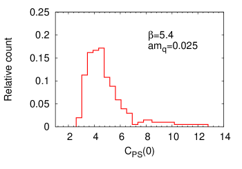
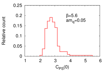
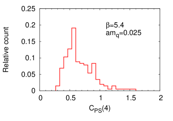
Figure 1: The distribution of measurements of the PS correlator at distance zero for two representative run IDs 6 (left) and 14 (right). The ID numbers associated with runs are given in Table 1. Such highly skewed distributions are seen to be generic.

Figure 2: The ratio of pion masses extracted with non-parametric bootstrap estimators of the correlator (labelled NP) and with Gaussian estimators (labelled G). The uncertainty in the ratio are obtained by repeating the bootstrap resampling and generating the distribution of the ratio. The ID numbers on the ordinate are associated with run parameters in Table 1.

The staggered pseudo-Goldstone pion is a good test-bed for exploring statistical techniques for two reasons. First, because masses are typically small, the relative uncertainty in the correlation function is small. Second, unlike other staggered hadrons, there is no opposite parity channel to complicate the analysis, and it is often sufficient to use a fitting form

$$C_{PS}(t)=A\cosh\left[m\left(\frac{aN_{t}}{2}-t\right)\right],$$ (1)

where $a$ is the lattice spacing, and $A$ and $ma$ are fit parameters.

We begin by examining the distribution of the measurements of the PS correlation function at fixed separation $t$. Two representative histograms of the measurements of the PS correlator are shown for each of $t=0$ and $t=4$ in Figure 1. They are highly skewed. We found that the set of configurations which give rise to measurements in the tail of the distribution of the correlator at $t=0$ are generically those which populate the tail at other $t$. Such long-tailed and skewed ensembles of the correlators are generic, in the sense that we saw such distributions for all 22 cutoffs and quark masses which we examined.

This is not an artifact of a lack of thermalization. The sequence of configurations which we used were thermalized according to global measurements like average plaquette or quark condensate. Moreover, the measurements which lie at the tails of the distribution are distributed throughout the runs, and not clustered together.

Non-Gaussian distributions of correlation functions have been sporadically reported in the literature nong . Unlike those, the distributions which we see are not log-normal. In fact, in this case even the logarithms of correlation functions have long-tailed distributions. An extreme example is for ID number 14 (see Table 1 for the association of ID numbers with run parameters). For this set the distribution of $\log C_{PS}(4)$, shown in the last panel of Figure 1, has skewness $-2.5$ and kurtosis 25. Systematic reports of distributions of correlators is not part of the standard analysis suite of lattice gauge theory. As a result, we do not know whether our observation is of greater generality.

We investigated the configurations which give measurements in the long tail of the distribution. Pion correlation functions measured on these configurations with different source locations do not have large values of the correlator for all locations of the source. In order to understand this, it is useful to think in terms of the eigenvalue decomposition of the correlators.

Suppose that $\lambda_{i}$ is an eigenvalue of the staggered Dirac operator, and the component of the eigenvector at site $x$ is $\left|{\lambda_{i}(x)}\right\rangle$, then

$$D_{xy}\left|{\lambda_{i}(y)}\right\rangle=\lambda_{i}\left|{\lambda_{i}(x)}\right\rangle,\qquad{\rm and}\qquad D^{-1}_{xy}=\sum_{i}\frac{1}{\lambda_{i}}\;\left|{\lambda_{i}(x)}\right\rangle\left\langle{\lambda_{i}(y)}\right|.$$ (2)

As a result, any local mesonic correlation function is given by

$$C(x,y)=\sum_{ij}\frac{1}{\lambda_{i}\lambda_{j}}\left\langle{\lambda_{i}(x)}\right|\gamma\left|{\lambda_{j}(x)}\right\rangle\left\langle{\lambda_{j}(y)}\right|\gamma\left|{\lambda_{i}(y)}\right\rangle,$$ (3)

where $\gamma$ is the spin-flavour matrix which enters the source for the meson under consideration. If a configuration has one or more eigenvalues $\lambda_{i}$ which are very small compared to the minimum eigenvalue in a generic configuration, then the correlation function becomes large. If, at the same time, the corresponding eigenvectors are localized, then $C(x,y)$ may not be equally large for all $x$ and $y$. This would imply that on these configurations some sources give much larger values of the correlator than others. Previous investigations have shown that the eigenvalues and eigenvectors have exactly this kind of behaviour in the presence of topological structures topology . This leads us to believe that topology is generally the reason for the skewed distributions which we see.

Since the tail of the distribution of measurements of the correlators is so long, it is not clear whether the central limit theorem applies. As a result, justification for the use of Gaussian statistics (labelled G), through the use of means, variances, and covariance matrices, is lacking. On the other hand, it is safe to use a non-parametric bootstrap analysis (labelled NP). This does have an effect on the determination of the mass, as we show in Figure 2. There is a tendency for NP to lead to a higher mass, although, as the figure shows, the discrepancy between the two methods is generally less than a 1-$\sigma$ effect.

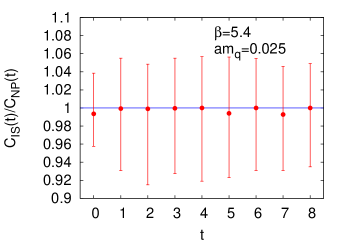
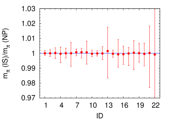
Figure 3: The first panel shows the ratio of pion correlators extracted with independent bootstrap estimators of the correlator at each $t$ (labelled IS) and using the same bootstrap configurations at all $t$ (labelled NP, as before) at a representative run ID 6. The second panel shows the comparison of masses extracted from the two different estimators of the correlators.

ID	$L/a$	$\beta$	$am_{q}$	S	$am_{\pi}({\rm NP\/})$	$am_{\pi}({\rm IS\/})$
1	16	5.2875	0.1	50	0.7899 (27)	0.7904 (23)
2	16	5.2875	0.05	50	0.5753 (23)	0.5756 (27)
3	16	5.2875	0.025	70	0.4159 (26)	0.4161 (27)
4	16	5.2875	0.015	50	0.3241 (24)	0.3240 (34)
5	16	5.4	0.05	75	0.6033 (47)	0.6030 (54)
6	16	5.4	0.025	51	0.4376 (61)	0.4376 (71)
7	24	5.4	0.015	51	0.3500 (18)	0.3504 (21)
8	32	5.4	0.01	40	0.2922 (17)	0.2925 (12)
9	16	5.5	0.05	50	0.6184 (91)	0.6177 (93)
10	24	5.5	0.025	101	0.4463 (22)	0.4459 (22)
11	28	5.5	0.015	120	0.3542 (19)	0.3541 (21)
12	32	5.5	0.01	40	0.2896 (21)	0.2894 (30)
13	32	5.5	0.005	50	0.2129 (39)	0.2124 (43)
14	24	5.6	0.05	55	0.5938 (29)	0.5935 (27)
15	24	5.6	0.025	103	0.4255 (66)	0.4246 (78)
16	28	5.6	0.015	120	0.3299 (49)	0.3302 (56)
17	32	5.6	0.01	40	0.2682 (42)	0.2685 (44)
18	32	5.6	0.005	50	0.1973 (45)	0.1965 (30)
19	32	5.6	0.003	105	0.1506 (25)	0.1513 (24)
20	24	5.7	0.025	59	0.3954 (73)	0.3956 (59)
21	32	5.7	0.005	50	0.1751 (57)	0.1738 (55)
22	32	5.7	0.003	50	0.134 (13)	0.134 (19)

Table 1: Comparison of pion masses extracted by the two methods labelled NP and IS, whose explanations are given in the text.

The molecular dynamics time separation between successive stored configurations which we used are larger than those used before for naive staggered quark simulations covmat ; milc38 ; milc42 ; col67 , and are typical of those used today. Additive increase of the MD time separation decreases autocorrelations exponentially. So it is worthwhile performing the analysis in which the correlation function at each distance is re-sampled independently.

Such a comparison is shown in the first panel of Figure 3 for the PS correlator in one of our simulations. The ratio of the correlation function obtained through independent sampling (labelled IS) and that obtained using our usual sampling (labelled NP as before) is completely consistent with unity at all separations. This conclusion is true for all sets of simulations we have made. A comparison of the masses obtained by the two methods is shown in Figure 3 through the ratio of the masses. As expected from the behaviour shown in the first panel, the masses are not changed by the sampling of the correlator. The pion masses estimated using these two methods are collected in Table 1. From the Table one also sees that our exploration of statistical methods covered a very wide range of pion masses in lattice units.

III The vector

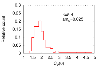
Figure 4: The distribution of measurements of the local vector correlators at distance zero for the representative run IDs 6 and 14 seem to be non-Gaussian. The configurations which give rise to the measurements at the tail of these distributions are generally those which populate the tail of the PS correlator.

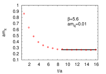
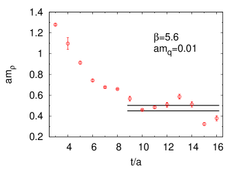
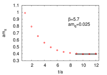
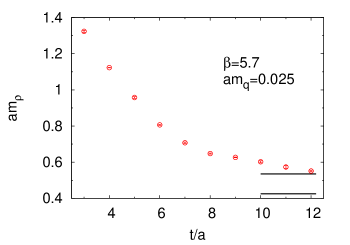
Figure 5: Local masses for pions and vector mesons in some representative runs. The best fit masses are shown along with the local masses. For pions the band shows the 68% statistical uncertainty band. For the vector meson the band is due to the systematic uncertainties, which happen to be larger than the statistical uncertainty. For $\beta=5.7$, $am_{\rho}$ is extracted after taking into account the excited state contribution.

ID	$\beta$	$am_{q}$	Single mass fit		Two masses fit
			$am_{\rho}({\rm NP\/})$	$am_{\rho}({\rm IS\/})$	$am_{\rho}({\rm NP\/})$	$am_{\rho}({\rm IS\/})$
1	5.2875	0.1	1.464 (7)	1.462 (8)
2	5.2875	0.05	1.336 (16)	1.340 (12)
3	5.2875	0.025	1.289 (6)	1.288 (6)
5	5.4	0.05	1.286 (4)	1.286 (3)
6	5.4	0.025	1.177 (9)	1.177 (12)
7	5.4	0.015	1.118 (6)	1.117 (6)
9	5.5	0.05	1.046 (9)	1.044 (9)
10	5.5	0.025	0.904 (4)	0.904 (4)
14	5.6	0.05	0.844 (4)	0.844 (5)	0.820 (19) (4)	0.819 (17) (6)
15	5.6	0.025	0.638 (2)	0.639 (4)	0.572 (16) (71)	0.565 (28) (79)
16	5.6	0.015	0.595 (4)	0.595 (4)	0.577 (15) (14)	0.571 (11) (26)
17	5.6	0.01	0.475 (14)	0.476 (13)
18	5.6	0.005	0.420 (18)	0.415 (18)	0.277 (39) (24)	0.291 (53) (24)
20	5.7	0.025	0.568 (3)	0.569 (5)	0.482 (28) (53)	0.480 (26) (55)
22	5.7	0.003	0.418 (11)	0.417 (8)	0.306 (36) (53)	0.304 (28) (72)

Table 2: Comparison of vector masses extracted by the methods NP and IS, for various ID numbers. The IDs and the labels on masses have the same meanings as in Table 1. In several cases the plateau in the local masses was too short to trust the single mass staggered fits, and the first excited state (and its staggered partner) was added to the fit. Data sets excluded from the table are too noisy for a stable fit.

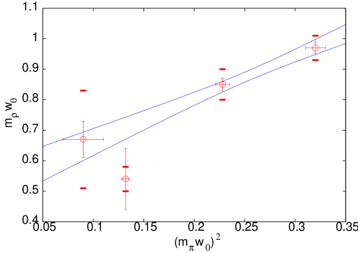
Figure 6: $m_{\rho}w_{0}$ as a function of $(m_{\pi}w_{0})^{2}$. The fat bars show systematic uncertainties; thin for statistical uncertainty. The blue lines show the 68% uncertainty band of a linear extrapolation fitted to the four data points shown here.

On examining the distributions of other meson correlation functions, we found that they are skewed in general. We show examples for the vector correlator in Figure 4. The tails of these distributions generally come from the same configurations as for the pion. As before, we take account of this skewness by using the methods, NP and IS, explored in the previous section.

The analysis of these correlation functions is more complex than that of the pseudo-Goldstone pion because the correlator contains an oscillating staggered piece

$$C_{V}(t)=A\cosh\left[m\left(\frac{aN_{t}}{2}-t\right)\right]+(-1)^{t/a}A^{\prime}\cosh\left[m^{\prime}\left(\frac{aN_{t}}{2}-t\right)\right],$$ (4)

where $a$ is the lattice spacing. We extract effective masses by using four successive values of $t$ to extract the four parameters. We looked for plateaus in such effective masses, and fitted the correlation function above within the range of the plateau. The statistical uncertainty in the fitted mass, $ma$, was obtained using a pair of nested bootstraps. For each set of re-samplings of the correlation function, the fit returned a value of the parameters being fitted. A further bootstrap over this process gave a distribution of the parameters. This was used to estimate parameter uncertainty in the usual way. There are also systematic uncertainties in the measurement. The major uncertainty comes from having to choose the range of the fit. We quote a systematic uncertainty on the fitted parameters as the maximum difference in the estimator of the mass when varying the end points of fit range by one lattice unit.

As one can see from the local masses in Figure 5, the region over which a fit can be performed is significantly shorter for the vector meson than for the pion. The lack of perfect overlap with the ground state limits the smallest values of $t$ which we can use in the fit. As is visible in the figures, this is not necessarily a more stringent cutoff for vectors than for pions. However, since the vector mass is larger, the correlator falls faster, and the signal to noise ratio deteriorates, limiting the largest $t$ which we can use. This large-$t$ problem can be beaten only with statistics, and therefore represents a hard CPU limitation. Instead, as is common in the literature, we try to use the small-$t$ information. Since the correlator couples to a tower of states, it gets a contribution in the form in eq. (4) from each state. Techniques for extracting ground and excited states simultaneously have been explored since long excited . Notable developments are the use of variational methods with many different forms of the source variational and Bayesian fitting bayes .

Here we use the technically simpler alternative method which uses a fit of two (four, with staggering) masses to the effective masses. Since the number of fit parameters doubles, one has to take a sufficiently large interval in $t$ to obtain a statistical test of the goodness of fit. Clearly, there are two sources of systematic uncertainties: first in determining the range over which the fit is performed, and second in choosing the $t$ with which to associate the effective mass which is being fitted. As before, we vary the fit interval by one unit at each end point. We also let the effective mass be associated with every separation which was used to determine it. The maximum variation in $ma$ obtained with these changes is quoted as a systematic uncertainty in this method.

Run IDs 3, 15 and 20 of Table 1 and Table 2 can be compared with previous measurements of masses reported in the literature milc38 ; milc42 ; col67 . In all three cases we find good agreement of previously quoted values of $am_{\pi}$ with the results we report in Table 1. We also find that the previously reported results on $am_{\rho}$ are in reasonable agreement with the vector masses we extract with single mass fits Table 2.

Since we have previously determined the Wilson flow scale $w_{0}/a$, we can examine our results for $am_{\rho}$ also in terms of $m_{\rho}w_{0}$. In Figure 6 we plot data on $m_{\rho}w_{0}$ as a function of $m_{\pi}w_{0}$ for the four smallest pion masses we used at the finest lattices possible. The coarsest lattice spacing among these corresponds to $a<w_{0}/1.7$. Since $m_{\pi}^{2}$ is proportional to a renormalized quark mass, when this is small enough, $m_{\rho}$ should be linear in this. Although the errors at the smallest quark masses are rather large, the data seems to fall the range where the linear extrapolation seems reasonable. In view of this, we fitted an extrapolation function for $m_{\rho}w_{0}$ linear in terms of $(m_{\pi}w_{0})^{2}$. The 68% uncertainty band on this extrapolation are also shown in Figure 6.

The slope of the extrapolation may be captured in the quantity

$$S_{\rho}=2\;\frac{m_{\rho}w_{0}(m_{\pi}w_{0}=0.4)-m_{\rho}w_{0}(m_{\pi}w_{0}=0.3)}{m_{\rho}w_{0}(m_{\pi}w_{0}=0.4)+m_{\rho}w_{0}(m_{\pi}w_{0}=0.3)}.$$ (5)

The fit shown in Figure 6 gives $S_{\rho}=0.14\pm 0.08$. With our set of simulations we are unable to remark on the possible lattice spacing dependence of this slope. A previous estimate of the ratio $w_{0}/\sqrt{t_{0}}$ with this set of simulations showed that a smooth limit is reached at $a\simeq w_{0}/2$ prev . While this could be taken as an indication that the slope parameter we have determined is close to its continuum value, it would be useful to check this in future.

With this fit we can extrapolate self-consistently to the physical $m_{\pi}$, and there use the physical value of $m_{\rho}$ to extract $w_{0}$ in physical units. We quote a statistical uncertainty in the extrapolation; this arises from the statistical uncertainty in the mass measurements. We also quote a systematic uncertainty which is the maximum difference between this extrapolation and the two obtained by leaving out of the fits either the measurement at the smallest or the largest $m_{\pi}$. This gives $w_{0}=0.14\pm 0.02\pm 0.01$ fm, where the first uncertainty is statistical and the second is systematic. This extraction of the scale $w_{0}$ is subject to the same caveats as the computations of the slope parameter $S_{\rho}$.

IV Conclusions

$\beta$	$ma$	$N_{s}$	Machine	Traj	Statistics	$w_{0}/a$	$am_{\pi}$	$am_{\rho}$	$m_{\pi}w_{0}$	$m_{\rho}w_{0}$
		$L/a$		(MD)	$T_{0}+T\times N$
5.2875	0.1	16	V	1	$400+10\times 50$	0.6112 (4)	0.790 (2)	1.462 (8) (7)	0.483 (1)	0.894 (5) (4)
	0.05	16	V	1	$780+10\times 50$	0.6354 (6)	0.576 (3)	1.340 (12) (7)	0.366 (2)	0.851 (8) (4)
	0.025	16	V	1	$200+15\times 70$	0.6539 (1)	0.416 (3)	1.288 (6) (–)	0.2714 (13)	0.842 (4) (–)
	0.015	16	V	1	$400+10\times 50$	0.6608 (5)	0.324 (3)	—	0.214 (2)	—
5.4	0.05	16	V	2	$200+20\times 75$	0.8418 (14)	0.603 (5)	1.286 (3) (2)	0.508 (4)	1.082 (3) (2)
	0.025	16	V	1	$400+10\times 51$	0.9264 (21)	0.438 (7)	1.177 (12) (23)	0.406 (6)	1.09 (1) (2)
	0.015	24	V	2	$400+10\times 50$	0.9600 (9)	0.354 (2)	1.117 (6) (10)	0.340 (2)	1.072 (6) (10)
	0.01	32	G	2	$200+20\times 40$	0.9922 (7)	0.292 (1)	—	0.290 (1)	—
5.5	0.05	16	V	1	$200+20\times 50$	1.1689 (40)	0.618 (9)	1.044 (9) (88)	0.72 (1)	1.22 (1) (10)
	0.025	24	V	1	$1680+10\times 101$	1.2651 (18)	0.446 (2)	0.904 (4) (11)	0.564 (3)	1.144 (5) (14)
	0.015	28	G	2	$400+10\times 120$	1.3302 (13)	0.354 (2)	—	0.471 (3)	—
	0.01	32	G	2	$200+20\times 40$	1.3771 (16)	0.289 (3)	—	0.398 (4)	—
	0.005	32	BG	1	$250+10\times 50$	1.4254 (37)	0.212 (4)	—	0.302 (6)	—
5.6	0.05	24	V	1	$400+10\times 55$	1.4850 (26)	0.594 (3)	0.819 (17) (6)	0.882 (5)	1.22 (2) (1)
	0.025	24	V	1	$1700+10\times 48$	1.6007 (33)	0.425 (8)	0.565 (28) (79)	0.68 (1)	0.90 (4) (13)
	0.015	28	G	2	$400+10\times 120$	1.7087 (25)	0.330 (6)	0.571 (11) (26)	0.56 (1)	0.97 (2) (4)
	0.01	32	G	2	$200+20\times 40$	1.7814 (36)	0.268 (4)	0.476 (13) (26)	0.477 (7)	0.85 (2) (5)
	0.005	32	BG	1	$300+10\times 50$	1.8547 (71)	0.196 (3)	0.291 (53) (24)	0.363 (6)	0.54 (10) (4)
	0.003	32	BG	1	$600+5\times 105$	1.8824 (32)	0.151 (2)	—	0.284 (4)	—
5.7	0.025	24	V	1	$530+10\times 59$	1.9645 (48)	0.396 (5)	0.480 (26) (55)	0.78 (1)	0.94 (5) (11)
	0.005	32	BG	1	$370+10\times 50$	2.1470 (73)	0.174 (5)	—	0.37 (1)	—
	0.003	32	BG	1	$300+10\times 50$	2.2103 (162)	0.13 (2)	0.304 (28) (72)	0.30 (4)	0.67 (6) (16)

Table 3: A summary of our scale setting measurements. The scale setting by $w_{0}$ was reported in prev . We have updated the pion masses presented in that study by reporting here the results of the analysis technique IS. For $m_{\rho}$ the statistical uncertainty are given before the systematic uncertainty.

In Section II we have reported extensively on the statistical analysis of masses. We observed that the distributions of correlation functions are strongly skewed, and a Gaussian analysis of the sample can not be justified. We found that bootstrap estimates, which do not assume any particular form of the distribution function, of the correlation functions and their errors give sensible results. We are not aware of earlier systematic reports on the distribution of measurements of correlation functions. We found that the masses obtained through independent bootstrap sampling of the correlator at each $t$ (called IS here) give results in complete agreement with sampling at all $t$ together (which we called NP). This is shown by the detailed compilation of results in Table 1 and Table 2.

The basic results we report in this paper are collected in Table 3. The measurements of $w_{0}$ were reported in prev ; they are included here for completeness. The pion and rho masses reported here are obtained using the IS sampling technique. Where older results covmat ; milc38 ; milc42 ; col67 are available, they agree with ours within statistical errors. Our results cover a wider range of lattice spacing and renormalized quark mass than was available for $N_{f}=2$ naive staggered quarks earlier. Our best estimate of the slope of the rho mass with the pion mass is

$$S_{\rho}=0.14\pm 0.08$$ (6)

where $S_{\rho}$ is defined in eq. (5).

Since we have earlier determined the scale $w_{0}/a$ at these bare parameters, we can now use these mass measurements to estimate the scale $w_{0}$ from the vector meson mass. Extrapolation to the physical pion mass yields the value

$$w_{0}=0.14\pm 0.02\pm 0.01{\rm\ fm},$$ (7)

where the first uncertainty is due to statistical uncertainties in the extraction of masses, and the second from an estimate of the uncertainty in the extrapolation to physical pion mass. This value for $N_{f}=2$ naive staggered quarks should be compared to the value $w_{0}=0.13^{+0.01}_{-0.02}$ fm, obtained earlier by a comparison with scale setting using the Lepage-Mackenzie method for the extraction of $\Lambda_{\overline{\scriptscriptstyle MS}}$ prev . Since the earlier extraction could require better control of UV artifacts than available at present, the current extraction, using a long-distance measurement, is an useful alternative method. It would be interesting to verify this estimate using other scales in future.

We also point out that an extraction of $w_{0}$ for $N_{f}=2$ clover quarks using $f_{K}$ to set the scale yields a larger value, namely $w_{0}=0.1757\pm 0.0013$ fm, where the uncertainty is statistical bruno . While the difference is not large or statistically very significant, it is intriguing. Tracing the source of this difference will certainly allow us to understand the continuum limits of various fermion measurements better.

Appendix A Distribution of sample medians

Suppose $r$ is a real random variate with distribution $f(r)$, and let $\mu$ be the population median. The cumulative distribution of $r$ is

$$F(r)=\int_{-\infty}^{r}f(t)dt,$$ (8)

where $F(\infty)=1$, $F(-\infty)=0$, and $F(\mu)=1/2$. If we draw $2n+1$ samples from the population and find that the median of the sample is $z$, then the probability of this being so is

$$g(z)={{2n+1}\choose n}\left\{F(z)[1-F(z)]\right\}^{n}f(z).$$ (9)

When $n$ is large enough, we expect $z$ to be close enough to $\mu$ so that the Taylor expansion

$$F(z)=\frac{1}{2}+f(\mu)(z-\mu)+\frac{1}{2}f^{\prime}(\mu)(z-\mu)^{2}+\cdots$$ (10)

converges sufficiently quickly. Then, using Stirling’s approximation in the binomial coefficient, we find that

$$\log g(z)\simeq-4n[f(\mu)]^{2}(z-\mu)^{2}+\cdots$$ (11)

This proves that $g(z)$ is Gaussian with mean $\mu$ and variance of $1/(8n[f(\mu)]^{2})$. The error in the estimate of $\mu$ therefore decreases as $1/\sqrt{n}$. This result is attributed to Laplace stigler . The proof given here is an adaptation of one from millers .

This construction fails when $f(\mu)=0$. Then, retaining the next term in the expansion, one can prove that $g(z)$ is even narrower. Such constructions fail completely when $f(r)$ vanishes identically in a region around $r=\mu$, so that a Taylor expansion of eq. (10) is impossible. However, this class of probability densities is different than that for which the central limit theorem fails. An instructive example with such a pathology is

$$f(r)=\frac{1}{2}\left[\delta(r)+\delta(r-1)\right].$$ (12)

References

-
(1)
For reviews, see
R. Sommer, PoS LATTICE2013 (2014) 015 [arxiv:1401.3270];
R. Sommer and U. Wolff, Nucl. Part. Phys. Proc. 261–262 (2015) 155 [arxiv:1501.01861]. - (2) S. Datta et al., Phys. Rev. D92 (2015) 9, 094509.
- (3) T. A. DeGrand and C. E. DeTar, Phys. Rev. D34 (1986) 2469.
- (4) B. Efron, The Jackknife, the Bootstrap and Other Resampling Plans, (1982) SIAM Monograph on Applied Mathematics.
- (5) Among the exceptions is A. Borici, Nucl. Phys. Proc. Suppl. 129 (2004) 817 [hep-lat/0309044].
- (6) S. Gupta, N. Karthik and P. Majumdar, Phys. Rev. D90 (2014) 3, 034001.
-
(7)
R. V. Gavai, S. Gupta and R. Lacaze, Phys. Rev. D77 (2008) 114506;
T. G. Kovacs, F. Pittier, Phys. Rev. Lett. 105 (2010) 192001;
V. Dick et al., Phys. Rev. D91 (2015) 9, 094504. -
(8)
M. G. Endres et al., sl PoS LATTICE2011 (2011) 017 [arXiv:1112.4023];
E. B. Gregory et al., Phys. Rev. D86 (2012) 014504;
T. DeGrand, Phys. Rev. D86 (2012) 014512. - (9) S. Gottlieb et al., Phys. Rev. D38 (1988) 2245.
- (10) K. M. Bitar et al., Phys. Rev. D42 (1990) 3794.
- (11) F. R. Brown et al., Phys. Rev. Lett. 67 (1991) 1062.
-
(12)
Y. Iwasaki et al., Nucl. Phys. Proc. Suppl. 30 (1993) 297;
S. M. Catterall et al., Phys. Lett. B 321 (1994) 246;
Dong Chen et al., Nucl. Phys. Proc. Suppl. 47 (1996) 382. -
(13)
C. Michael, Nucl. Phys. B 259 (1985) 58;
M. Luscher and U. Wolff, Nucl. Phys. B 339 (1990) 222. -
(14)
D. Makovoz, Nucl. Phys. Proc. Suppl. 53 (1997) 246;
G. P. Lepage et al., Nucl. Phys. Proc. Suppl. 106 (2002) 12;
C. Morningstar, Nucl. Phys. Proc. Suppl. 109A (2002) 185. - (15) M. Bruno and R. Sommer, PoS, LATTICE2013 (2014) 321 [arxiv:1311.5585].
- (16) S. M. Stigler, Biometrika, 60 (1973) 439.
-
(17)
A. Merberg and S. J. Miller, (2008) in
https://web.williams.edu/Mathematics/sjmiller/public_html/BrownClasses/162/Handouts/MedianThm04.pdf