FinInG: a package for Finite Incidence Geometry

John Bamberg, Anton Betten, Philippe Cara, Jan De Beule,
Max Neunhöffer, and Michel Lavrauw

Abstract

FinInG is a package for computation in Finite Incidence Geometry. It provides users with the basic tools to work in various areas of finite geometry from the realms of projective spaces to the flat lands of generalised polygons. The algebraic power of GAP is exploited, particularly in its facility with matrix and permutation groups.

Keywords: Finite classical groups, finite projective spaces, finite classical polar spaces, coset geometries, finite generalised polygons, algebraic varieties, finite affine spaces, morphisms.

1 Finite incidence geometry on the computer

FinInG [1] is a new share package for GAP [7]. It is designed to provide an environment to explore various finite geometrical structures, such as projective spaces, affine spaces, classical polar spaces, coset geometries and their diagrams and generalised polygons; allowing an integrated use of the automorphism groups and exploring geometrical relations between different geometries via incidence preserving morphisms. The use of automorphism groups is connected with the existing primary functionality of GAP as a computer algebra package chiefly concerned with computing with groups. The algebraic power of GAP is especially exploited when finite fields are involved, and when considering affine and projective algebraic varieties. Our package interfaces with the packages GRAPE [14] and DESIGN [13] which is especially useful when working with generalised polygons and purely combinatorial incidence structures. The representation of an automorphism group of a projective space relies on an implementation of collineations of a projective space as semilinear maps of the underlying vector space, and this is done in conjunction with the packages GenSS and Orb [12, 10] that provide sophisticated algorithms for enumeration of orbits, stabilisers, and stabiliser chains. Finally the package Forms [2] enables us to provide the user with the possibility to construct classical polar spaces from a user-defined sesquilinear or quadratic form, computing the necessary coordinate transformations on the fly. This approach results in a user-friendly and intuitive package providing generic functionality for exploring the most commonly studied finite incidence structures and their automorphism groups.

Other good systems are available for incidence geometry but often focus on the efficient handling of particular cases, rather than on the generic approach which is central in FinInG. The system MAGMA [3], for example, is renown as a system for computational group theory. It contains an implementation of projective planes, some substructures, coset geometries and related functionality. The computation of the automorphism group of a projective plane is done very efficiently, however, it is always returned as a permutation group on the points of the plane. The creation of a coset geometry is based on a given permutation group, which is very efficient, but which makes it more difficult for the user to use, for example, matrix groups occurring from (say) the automorphism group of a classical polar space. For the student starting with finite incidence geometry, or the (experienced) researcher interested in exploring a particular incidence structure using a computer, this approach might be a hurdle.

This explains the basic philosophy of FinInG: to construct an incidence structure (together with an automorphism group) in its natural representation, where the user decides what natural actually means! For example, a conic with a particular equation can easily be constructed, or a coset geometry arising from a matrix group or finitely presented group instead of a permutation group. Once objects in a certain category have been constructed, their behaviour is independent of their representation. Furthermore, many well studied geometries are considered in their standard representation, together with straight-forward methods for switching from one representation to another.

⬇

gap> map := KleinCorrespondence(7);

<geometry morphism from <lines of ProjectiveSpace(3, 7)> to

gap> r := Range(map);

gap> hyp := AmbientGeometry(r);

Q+(5, 7): x_1*x_6+x_2*x_5+x_3*x_4=0

gap> klein := HyperbolicQuadric(5,7);

Q+(5, 7)

gap> EquationForPolarSpace(klein);

x_1*x_2+x_3*x_4+x_5*x_6

gap> map := KleinCorrespondence(klein);

gap> morphism := IsomorphismPolarSpaces(hyp,klein);

<geometry morphism from <Elements of Q+(5, 7): x_1*x_6+x_2*x_5+x_3*x_4=0> to

1.1 Klein Correspondence

⬇

gap> L := SimpleLieAlgebra("E",6,Rationals);

gap> rs := RootSystem(L);

gap> w := WeylGroup(rs);

gap> gens := GeneratorsOfGroup(w);;

gap> parabolics := List(gens, x -> Group(Difference(gens, [x])));

[ <matrix group with 5 generators>, <matrix group with 5 generators>,

<matrix group with 5 generators>, <matrix group with 5 generators>,

<matrix group with 5 generators>, <matrix group with 5 generators> ]

gap> g := Group(gens);

gap> cg := CosetGeometry(g,parabolics);

CosetGeometry( Group(

[ [ [ -1, 0, 1, 0, 0, 0 ], [ 0, 1, 0, 0, 0, 0 ], [ 0, 0, 1, 0, 0, 0 ],

[ 0, 0, 0, 1, 0, 0 ], [ 0, 0, 0, 0, 1, 0 ], [ 0, 0, 0, 0, 0, 1 ] ],

[ [ 1, 0, 0, 0, 0, 0 ], [ 0, -1, 0, 1, 0, 0 ], [ 0, 0, 1, 0, 0, 0 ],

[ 0, 0, 0, 1, 0, 0 ], [ 0, 0, 0, 0, 1, 0 ], [ 0, 0, 0, 0, 0, 1 ] ],

[ [ 1, 0, 0, 0, 0, 0 ], [ 0, 1, 0, 0, 0, 0 ], [ 1, 0, -1, 1, 0, 0 ],

[ 0, 0, 0, 1, 0, 0 ], [ 0, 0, 0, 0, 1, 0 ], [ 0, 0, 0, 0, 0, 1 ] ],

[ [ 1, 0, 0, 0, 0, 0 ], [ 0, 1, 0, 0, 0, 0 ], [ 0, 0, 1, 0, 0, 0 ],

[ 0, 1, 1, -1, 1, 0 ], [ 0, 0, 0, 0, 1, 0 ], [ 0, 0, 0, 0, 0, 1 ] ],

[ [ 1, 0, 0, 0, 0, 0 ], [ 0, 1, 0, 0, 0, 0 ], [ 0, 0, 1, 0, 0, 0 ],

[ 0, 0, 0, 1, 0, 0 ], [ 0, 0, 0, 1, -1, 1 ], [ 0, 0, 0, 0, 0, 1 ] ],

[ [ 1, 0, 0, 0, 0, 0 ], [ 0, 1, 0, 0, 0, 0 ], [ 0, 0, 1, 0, 0, 0 ],

[ 0, 0, 0, 1, 0, 0 ], [ 0, 0, 0, 0, 1, 0 ], [ 0, 0, 0, 0, 1, -1 ] ] ]) )

1.2 An apartment in a building of type

E_{6}

Example 1.1 illustrates the Klein correspondence (between the lines of a $3$ -dimensional projective space and the points of a hyperbolic quadric in $5$ dimensions). The example shows the default behaviour and the possibility to employ a user-defined form for the Klein quadric.

Example 1.2, illustrates the construction of an apartment in a building of type $\mathrm{E}_{6}$ , based on existing GAP functionality of root systems and Lie algebras.

2 Fundamentals of FinInG

First of all, a set of new data structures, which are type in GAP by the so-called categories, is provided in FinInG, summarized as follows.

•

FinInG Incidence geometries have their category, together with elementary operations.
•

Finite projective spaces, classical finite polar spaces, and some classical generalized polygons are incidence geometries whose elements are represented by sub spaces of a vector space over a finite field. They are called Lie geometries in FinInG. More particular operations are applicable on such geometries. As explained in the introduction, the user is free to choose a representation for a Lie geometry.
•

Generalised polygons are particular examples of point-line incidence geometries. Many examples in many different representations exist. FinInG provides a generic category, together with some particular operations, allowing the user to construct in a very natural way their desired geometry.
•

Coset geometries can be constructed from any group in their own category.
•

Finally affine spaces can also be constructed as objects in their dedicated category.

The automorphism groups of Lie geometries are naturally represented by semi-linear maps on the underlying vector space. FinInG provides category for such maps acting on the projective space. Groups generated by such maps can be constructed, functions representing the action on elements of a Lie geometry are provided, and actions can be computed, including nice monomorphisms. This part of FinInG is the direct link between the automorphism groups of Lie geometries and the available GAP operations for permutation groups.

Secondly fining provides efficient operations to compute orbits and (setwise) stabilisers of projective semilinear groups. These operations are based on the use of the packages orb, genss and cvec. Also from the algorithmic point of view, FinInG provides efficient methods to enumerate the the elements of finite classical polar spaces. Geometry morphisms can be constructed. This is especially powerfull combined with field reduction.

3 Incidence geometries

We follow [4] for the definitions of incidence structure and incidence geometry. An incidence structure $\mathcal{S}$ consists of a set of elements, a reflexive and symmetric relation $\operatorname{\mathrm{I}}$ on the elements and a type function from the set of elements to an index set (i.e., every element has a “type”). It satisfies the following axiom:

(i) no two different elements of the same type are incident.

If we forget the type function, an incidence structure is just a multipartite graph where adjacency is incidence. Note that every element is incident with itself, so there is a loop on each vertex. The type function turns the graph into a coloured graph. Assume that $\mathcal{S}$ is an incidence structure with type function $t$ with range $T=\{1,\ldots,n\}$ . Then we say that $\mathcal{S}$ has rank $n$ . A flag is a set $F$ of elements of $\mathcal{S}$ such that every two elements contained in $F$ are incident. Necessarily, $F$ cannot contain two elements of the same type, so $F$ contains at most $n$ elements. We call a flag maximal when no element of $\mathcal{S}$ is incident with all elements of $F$ , unless it is already contained in $F$ .

The term geometry, or incidence geometry, is interpreted broadly in this package. Particularly, an incidence geometry is an incidence structure satisfying the following axiom:

(ii) every maximal flag contains an element of each type.

In graph terminology, this means that every maximal clique contains an element of each colour.

Let $\mathcal{S}$ be an incidence structure of rank $n$ , and let $e$ be an element of type $i\in T$ . Let $j\in T\setminus\{i\}$ . Then the $j$ -shadow of $e$ is the set of elements of type $j$ incident with $e$ . Let $F$ be a flag of $\mathcal{S}$ then the $j$ -shadow of $F$ is the set of elements of type $j$ incident with all elements in $F$ . The residue of $F$ is the set of all elements of $\mathcal{S}$ not in $F$ but incident with all elements of $F$ , together with the induced geometrical structure. Hence, the residue of a maximal flag of an incidence geometry is empty. All geometries that can be constructed in FinInG are incidence structures. This terminology is consistently used, as illustrated in Example 3.1 for an “abstract” coset geometry and Example 3.2 for a projective space.

⬇

gap> involset:=[(1,2), (1,3), (3,4), (4,5), (4,6), (6,9), (6,10),

(7,10), (8,10)];;

gap> g:=Group(involset);;

gap> parabolics := List(involset, i -> Subgroup(g, Difference(involset, [i]) ) );;

gap> img:=CosetGeometry(g, parabolics);

CosetGeometry( Group( [ (1,2), (1,3), (3,4), (4,5), (4,6), (6,9),

( 6,10), ( 7,10), ( 8,10) ] ) )

gap> elements_type_2 := ElementsOfIncidenceStructure(img,2);

<elements of type 2 of CosetGeometry( Group(

[ (1,2), (1,3), (3,4), (4,5), (4,6), (6,9), ( 6,10), ( 7,10), ( 8,10) ]

) )>

gap> el2 := Random(elements_type_2);

<element of type 2 of CosetGeometry( Group(

[ (1,2), (1,3), (3,4), (4,5), (4,6), (6,9), ( 6,10), ( 7,10), ( 8,10) ]

) )>

gap> shad := ShadowOfElement(img,el2,3);

<shadow elements of type 3 in CosetGeometry( Group(

[ (1,2), (1,3), (3,4), (4,5), (4,6), (6,9), ( 6,10), ( 7,10), ( 8,10) ]

) )>

gap> el3 := Random(shad);

<element of type 3 of CosetGeometry( Group(

[ (1,2), (1,3), (3,4), (4,5), (4,6), (6,9), ( 6,10), ( 7,10), ( 8,10) ]

) )>

gap> IsIncident(el2,el3);

true

gap> flag := FlagOfIncidenceStructure(img,[el2,el3]);;

gap> shad := ShadowOfFlag(img,flag,4);

<shadow elements of type 4 in CosetGeometry( Group(

[ (1,2), (1,3), (3,4), (4,5), (4,6), (6,9), ( 6,10), ( 7,10), ( 8,10) ]

) )>

3.1 Elements and shadows in a coset geometry

⬇

gap> pg := PG(5,7);

ProjectiveSpace(5, 7)

gap> Rank(pg);

gap> line := Random(Lines(pg));

gap> shadowplanes := ShadowOfElement(pg,line,3); #planes are type 3

gap> plane := Random(shadowplanes);

gap> planepoints := ShadowOfElement(pg,plane,1); #planes are type 1

gap> p := Random(planepoints);

gap> flag := FlagOfIncidenceStructure(pg,[p,plane]);

gap> shadowlines := ShadowOfFlag(pg,flag,2);

3.2 Elements and shadows in a projective space

4 Lie geometries

Example 3.2 brings us to the Lie geometries. A Lie geometry, is an incidence geometry whose automorphism group is a (subgroup of) a group of Lie type in its natural representation. One common fact about Lie geometries is that their elements are represented by subspaces of a vector space. All the collineations are induced by semilinear maps of the underlying vector space. So a finite Lie geometry is a geometry for which the elements are subspaces of some projective space over a finite field, and with symmetrised set-theoretic containment as incidence. Hence, a Lie geometry is naturally embedded in a projective space. These principles are used in FinInG to implement Lie geometries. Currently the following Lie geometries are readily implemented in FinInG:

•

projective spaces,
•

classical polar spaces, and,
•

the so-called classical generalised hexagons and octagons.

Elements of Lie geometries are also called subspaces. Subspaces have a (projective) dimension, and subspaces of projective dimension $0,1,2,3$ are called points, lines, planes, solids, respectively. In FinInG the default type set is $\{1,\ldots,n\}$ and the type of an element is its projective dimension plus one. Some handy shortcuts for the operation ShadowOfElements are implemented, so that given a point $p$ , Lines(p) is equivalent with ShadowOfElement(pg,p,2). Basic operations such as Meet and Span, illustrated in Example 4.1, rely on operations to deal with subspaces of the underlying vector space of the Lie geometry.

⬇

gap> pg := PG(8,9);

ProjectiveSpace(8, 9)

gap> ElementsOfIncidenceStructure(pg,1);

gap> Points(pg);

gap> Lines(pg);

gap> Planes(pg);

gap> Solids(pg);

gap> ElementsOfIncidenceStructure(pg,5);

<proj. 4-subspaces of ProjectiveSpace(8, 9)>

gap> plane := Random(Planes(pg));

gap> Solids(plane);

gap> line := Random(Lines(pg));

gap> Span(line,plane);

gap> Meet(line,plane);

< empty subspace >

gap> hyperplane := Random(Hyperplanes(pg));

gap> Meet(line,hyperplane);

gap> Span(line,hyperplane);

ProjectiveSpace(8, 9)

4.1 Lie geometries: elements of projective spaces

A polar space is a partial linear space satisfying the so-called one-or-all axiom: given a point $P$ and a line $l$ , $P$ not incident with $l$ , there is either exactly one line incident with $P$ meeting $l$ in a point, or points of $l$ span with $P$ a line of the polar space. The classical polar spaces are constructed from vector spaces equipped with a form as follows. Consider a vector space $V(d+1,q)$ equipped with a non-degenerate sesquilinear form $f$ , respectively non-singular quadratic form $f$ . The polar space $\mathcal{S}$ associated to the form $f$ is the geometry of which the elements are represented by the totally isotropic, respectively totally singular, subspaces with respect to the form $f$ . The rank of $\mathcal{S}$ equals the Witt index of the form $f$ . So we see that $\mathcal{S}$ is embedded in the projective space $\mathrm{PG}(d,q)$ . Sesquilinear and quadratic forms on a finite vector space have been classified. Up to coordinate transformation, they fall into three main classes.

1.

orthogonal polar spaces, associated with a quadratic form (which in odd characteristic is equivalent with a symmetric bilinear form);
2.

symplectic polar spaces, associated with an alternating bilinear form;
3.

hermitian polar spaces, associated with a unitary form.

The orthogonal polar spaces separate into three classes: parabolic quadrics (in even projective dimension), and elliptic and hyperbolic quadrics (in odd projective dimension).

Classical polar spaces can be constructed in several ways in FinInG. A user-defined sesquilinear or quadratic form can be used, but FinInG also provides shortcuts to classical polar spaces defined by a “standard form”. The following example illustrates this possibility. When appropriate, the connection with polarities of projective spaces can be explored. Example 4.2 illustrates some basic functionality for polar spaces as well.

⬇

gap> mat := [[0,0,0,1],[0,0,-2,0],[0,2,0,0],[-1,0,0,0]]*Z(5)^0;

[ [ 0*Z(5), 0*Z(5), 0*Z(5), Z(5)^0 ], [ 0*Z(5), 0*Z(5), Z(5)^3, 0*Z(5) ],

[ 0*Z(5), Z(5), 0*Z(5), 0*Z(5) ], [ Z(5)^2, 0*Z(5), 0*Z(5), 0*Z(5) ] ]

gap> form := BilinearFormByMatrix(mat,GF(25));

< bilinear form >

gap> ps := PolarSpace(form);

<polar space in ProjectiveSpace(

3,GF(5^2)): x1*y4+Z(5)^3*x2*y3+Z(5)*x3*y2-x4*y1=0 >

gap> Rank(ps);

gap> ps;

W(3, 25): x1*y4+Z(5)^3*x2*y3+Z(5)*x3*y2-x4*y1=0

gap> ps := EllipticQuadric(5,7);

Q-(5, 7)

gap> Rank(ps);

gap> phi := PolarityOfProjectiveSpace(ps);

gap> ps := ParabolicQuadric(4,4);

Q(4, 4)

gap> phi := PolarityOfProjectiveSpace(ps);

Error, no polarity of the ambient projective space can be associated to <ps>

4.2 Finite classical polar spaces: elementary operations

Lie geometries are naturally embedded in projective spaces. In FinInG this means that an element of a polar space, for example, is automatically an element of the ambient projective space. Example 4.3 demonstrates the philosophy of Lie geometries in FinInG.

⬇

gap> hexagon := SplitCayleyHexagon(3);

H(3)

gap> p := Random(Points(hexagon));

#I for Split Cayley Hexagon

#I Computing nice monomorphism...

#I Found permutation domain...

gap> lines := Lines(p);

gap> Size(lines);

gap> polarspace := AmbientPolarSpace(hexagon);

Q(6, 3): -x_1*x_5-x_2*x_6-x_3*x_7+x_4^2=0

gap> p2 := ElementToElement(polarspace,p);

gap> p2 in hexagon;

true

gap> lines2 := Lines(p2);

gap> Size(lines2);

gap> Collected(List(lines2,x->x in hexagon));

[ [ true, 4 ], [ false, 36 ] ]

gap> pg := AmbientSpace(hexagon);

ProjectiveSpace(6, 3)

gap> p3 := ElementToElement(pg,p);

gap> p3 in polarspace;

true

gap> p3 in hexagon;

true

gap> lines3 := Lines(p3);

gap> Collected(List(lines3,x->x in hexagon));

[ [ true, 4 ], [ false, 360 ] ]

gap> Collected(List(lines3,x->x in polarspace));

[ [ true, 40 ], [ false, 324 ] ]

4.3 Lie geometries embedded in projective spaces

5 Collineation groups of Lie geometries

A collineation of an incidence geometry $\mathcal{S}$ is a type preserving map from $\mathcal{S}$ to itself that preserves the incidence. Let $\mathrm{PG}(d,q)$ denote a $d$ -dimensional projective space over the finite field $\mathrm{GF}(q)$ . As we have seen in the previous section, the elements of $\mathrm{PG}(d,q)$ are represented by the subspaces of the $d+1$ -dimensional vector space $V(d+1,q)$ . By the Fundamental Theorem of Projective Geometry, each collineation of a projective space $\mathrm{PG}(d,q)$ is induced by a semilinear automorphism of $V(d+1,q)$ . The group of semilinear automorphisms of $V(d+1,q)$ is denoted by $\Gamma\mathrm{L}(d+1,q)$ , and an element of this group is completely determined by a non-singular matrix and an automorphism of the underlying field. The scalar matrices form a subgroup $\mathrm{Sc}(d+1,q)$ of the group $\Gamma\mathrm{L}(d+1,q)$ that acts trivially on the subspaces of $V(d+1,q)$ . The permutation group induced on the subspaces is the projective general semilinear group:

\mathrm{P}\Gamma\mathrm{L}(d+1,q)\cong\Gamma\mathrm{L}(d+1,q)/\mathrm{Sc}(d+1,q)\,.

The group $\mathrm{PGL}(d+1,q)$ is the subgroup of $\Gamma\mathrm{L}(d+1,q)$ induced by the linear automorphisms of $V(d+1q)$ . This group is called the projectivity group or homography group of $\mathrm{PG}(d,q)$ .

The projectivity groups are already implemented in GAP, but only as permutation groups.without the underlying geometry. W provide the implementation of collineation groups of projective spaces as groups induced by semilinear transformations of vector spaces. Note that an element of a Lie geometry is represented by a subspace of a vector space, which in FinInG is inturn represented as the row-space of a matrix. Let $M$ be an $(m+1)\times(d+1)$ -matrix over $\mathrm{GF}(q)$ of rank $m+1$ . The row-space of $M$ represents a subspace $\pi$ of $\mathrm{PG}(d,q)$ of projective dimension $m$ . Let $\phi$ be a semilinear automorphism of $V(d+1,q)$ represented by the matrix $A$ and the field automorphism $\theta$ . In FinInG, the image of $\pi$ under $\phi$ is the projective subspace represented by the matrix $M^{\prime}$ , with

M^{\prime}:=(MA)^{\theta}

The first example below shows the difference between the projectivity group that was already implemented in GAP and the projectivity group implemented in FinInG. The example also illustrates that accessing the collineation groups implemented in FinInG is naturally associated to the underlying incidence geometry.

⬇

gap> g1 := PGL(5,27);

gap> g2 := ProjectivityGroup(PG(4,27));

The FinInG projectivity group PGL(5,27)

gap> Order(g2);

22496309500661613496614846025474560

gap> g3 := CollineationGroup(PG(4,27));

The FinInG collineation group PGammaL(5,27)

gap> Order(g3);

67488928501984840489844538076423680

gap> GeneratorsOfGroup(g1)[1];

(20442,20467,20466,20465,20464,20463,20462,20461,20460,20459,20458,20457,

20456,20443,20455,20454,20453,20452,20451,20450,20449,20448,20447,20446,20445,

20444)(20468,21143,21116,21089,21062,21035,21008,20981,20954,20927,20900,

20873,20846,20495,20819,20792,20765,20738,20711,20684,20657,20630,20603,20576,

20549,20522)(20469,21169,21141,21113,21085,21057,21029,21001,20973,20945,

20917,20889,20861,20497,20833,20805,20777,20749,20721,20693,20665,20637,20609,

20581,20553,20525)(20470,21157,21129,21101,21073,21045,21017,20989,20961,

20933,20905,20877,20849,20496,20845,20817,20789,20761,20733,20705,20677,20649,

20621,20593,20565,20537)(20471,21144,21142,21114,21086,21058,21030,21002,

20974,20946,20918,20890,20862,20510,20821,20806,20778,20750,20722,20694,20666,

20638,20610,20582,20554,20526)(20472,21146,21117,21115,21087,21059,21031,

21003,20975,20947,20919,20891,20863,20511,20834,20794,20779,20751,20723,20695,

20667,20639,20611,20583,20555,20527)(20473,21147,21119,21090,21088,21060,

21032,21004,20976,20948,20920,20892,20864,20512,20835,20807,20767,20752,20724,

20696,20668,20640,20612,20584,20556,20528)(20474,21148,21120,21092,21063,

21061,21033,21005,20977,20949,20921,20893,20865,20513,20836,20808,20780,20740,

20725,20697,20669,20641,20613,20585,20557,20529)( [...] )

gap> GeneratorsOfGroup(g2)[1];

< a collineation: <cmat 5x5 over GF(3,3)>, F^0>

gap> GeneratorsOfGroup(g3)[1];

< a collineation: <cmat 5x5 over GF(3,3)>, F^0>

5.1 Projectivity groups

The next example shows how to construct a collineation of a projective space, and how to get the underlying matrix and field automorphism of a collineation.

⬇

gap> mat := [ [ Z(7^3)^115, Z(7^3)^164, Z(7^3)^189 ],

> [ Z(7^3)^146, Z(7^3)^279, Z(7^3)^215 ],

> [ Z(7^3)^58, Z(7^3)^322, Z(7^3)^260 ] ];

[ [ Z(7^3)^115, Z(7^3)^164, Z(7^3)^189 ],

[ Z(7^3)^146, Z(7^3)^279, Z(7^3)^215 ],

[ Z(7^3)^58, Z(7^3)^322, Z(7^3)^260 ] ]

gap> theta := FrobeniusAutomorphism(GF(7^3))^2;

FrobeniusAutomorphism( GF(7^3) )^2

gap> phi := ProjectiveSemilinearMap(mat,theta,GF(7^3));

< a collineation: <cmat 3x3 over GF(7,3)>, F^49>

gap> psi := Random(CollineationGroup(PG(2,2^3)));

< a collineation: <cmat 3x3 over GF(2,3)>, F^4>

gap> UnderlyingMatrix(psi);

gap> Unpack(last); # to get actual matrix from cvec

[ [ Z(2^3)^6, Z(2^3), Z(2)^0 ], [ Z(2^3)^2, Z(2^3)^4, Z(2^3)^2 ],

[ Z(2^3)^5, Z(2^3)^3, Z(2^3)^4 ] ]

gap> FieldAutomorphism(psi);

FrobeniusAutomorphism( GF(2^3) )^2

5.2 Constructing collineations of a projective space

Note that also the projective special homography groups are implemented in GAP as permutation groups, these are the groups of homographies where the underlying matrix has determinant one.

⬇

gap> PSL(3,49);

gap> SpecialHomographyGroup(PG(2,49));

The FinInG PSL group PSL(3,49)

gap> Order(last);

11072935641600

5.3 Special homography groups

Let $\mathcal{S}$ be a polar space defined by the sesquilinear form $f$ on the vector space $V(d+1,q)$ . Let $\varphi$ be a semilinear automorphism of $V(d+1,q)$ . If $\varphi$ preserves the zeroes of the form $f$ , that is,

f(u^{\varphi},v^{\varphi})=0\iff f(u,v)=0\quad\forall u,v\in V(d+1,q),

then $\varphi$ induces a collineation of $\mathcal{S}$ , and all collineations of $\mathcal{S}$ are induced by such automorphisms of $V(d+1,q)$ . If $\varphi$ preserves the values of the form $f$ , i.e., $\forall u,v:f(u^{\varphi},v^{\varphi})=f(u,v)$ , then the induced collineation is called an isometry of $\mathcal{S}$ . If $\varphi$ preserves the form $f$ up to a scalar, i.e., $\forall u,v:f(u^{\varphi},v^{\varphi})=\alpha f(u,v)$ and $\alpha$ is fixed, then the induced collineation is called a similarity. Finally, the special isometries are the isometries induced by a linear automorphism with determinant $1$ , i.e., an element of $\mathrm{SL}(d+1,q)$ . If $\mathcal{S}$ is a polar space with special isometry group $S$ , isometry group $I$ , similarity group $G$ and collineation group $\Gamma$ , respectively, then $S\leqslant I\leqslant G\leqslant\Gamma$ . Equalities can occur depending on the type of $\mathcal{S}$ . Table 1 provides an overview.

group/polar space	symplectic	hyperbolic	elliptic	parabolic	hermitian
special isometries	$\mathrm{PSp}(d,q)$	$\mathrm{PSO}^{+}(d,q)$	$\mathrm{PSO}^{-}(d,q)$	$\mathrm{PSO}(d,q)$	$\mathrm{PSU}(d,q^{2})$
isometries	$\mathrm{PSp}(d,q)$	$\mathrm{PGO}^{+}(d,q)$	$\mathrm{PGO}^{-}(d,q)$	$\mathrm{PGO}(d,q)$	$\mathrm{PGU}(d,q^{2})$
similarities	$\mathrm{PGSp}(d,q)$	$\mathrm{P\Delta O}^{+}(d,q)$	$\mathrm{P\Delta O}^{-}(d,q)$	$\mathrm{PGO}(d,q)$	$\mathrm{PGU}(d,q^{2})$
collineations	$\mathrm{P\Gamma Sp}(d,q)$	$\mathrm{P\Gamma O}^{+}(d,q)$	$\mathrm{P\Gamma O}^{-}(d,q)$	$\mathrm{P\Gamma O}(d,q)$	$\mathrm{P\Gamma U}(d,q^{2})$

Table 1: Collineation groups of finite classical polar spaces

All groups from Table 1 are constructed in FinInG as a collineation group of a finite classical polar space. Consistent with the basic philosophy of FinInG, such a geometry is determined by a user chosen sesquilinear/quadratic form. To compute the groups, we use the generators from [8], which are given with relation to a fixed sesquilinear/quadratic form, and apply the necessary coordinate transformations on the fly, using the package Forms.

⬇

gap> ps := HermitianPolarSpace(2,4);

H(2, 2^2)

gap> CollineationGroup(ps);

PGammaU(3,2^2)

gap> SpecialIsometryGroup(ps);

PSU(3,2^2)

gap> mat := IdentityMat(3,GF(9));

[ [ Z(3)^0, 0*Z(3), 0*Z(3) ], [ 0*Z(3), Z(3)^0, 0*Z(3) ],

[ 0*Z(3), 0*Z(3), Z(3)^0 ] ]

gap> form := QuadraticFormByMatrix(mat,GF(9));

< quadratic form >

gap> ps := PolarSpace(form);

gap> g := SimilarityGroup(ps);

#I Computing collineation group of canonical polar space...

gap> h := SimilarityGroup(ParabolicQuadric(2,9));

PGO(0,3,9)

5.4 Constructing collineation groups of finite classical polar spaces

6 Group actions for collineation groups of Lie geometries

The general mechanism in GAP to describe the action of the elements of a group $G$ on the elements of a set $A$ is through so-called action functions. An action function for the group $G$ and the set $A$ is a GAP function that takes two arguments, $g\in G$ and $a\in A$ , and returns the image of $a$ under $g$ (usually denoted as $a^{g}$ or $g(a)$ ). To explore group theoretical properties of the action of the group $G$ on the elements of a set $A$ , some generic GAP functions will compute a permutation representation of this action, which necessarily uses the action function. So for a given incidence geometry $\mathcal{S}$ , with a group of collineations $G$ , FinInG usually provides an action function for the group $G$ and the set of elements (of a given type) of $\mathcal{S}$ . For Lie geometries, FinInG provides the action function OnProjSubspaces. The following example illustrates its use.

⬇

gap> ps := ParabolicQuadric(4,3);

Q(4, 3)

gap> group := IsometryGroup(ps);

PGO(0,5,3)

gap> hom := ActionHomomorphism(group,Lines(ps),OnProjSubspaces);

gap> act := Image(hom);

Group([ (1,2)(3,5)(4,7)(6,10)(9,14)(11,17)(12,18)(15,21)(16,23)(19,22)(20,24)

(25,29)(27,28)(30,34)(33,38)(36,39), (1,3,6,11)(2,4,8,13,19,14,20,25,30,35,40,

18)(5,9,15,22,27,32,37,38,34,39,29,17)(7,12)(10,16)(21,26,31,36)(23,28,33) ])

6.1 Action of a collineation group on projective subspaces

In GAP, a nice monomorphism of an (abstract) group $G$ is a permutation representation of $G$ on a suitable action domain. Such a permutation representation makes it possible to use permutation group algorithms to explore properties of $G$ . If a nice monomorphism is available for an abstract group, a complete set of GAP functions will perform much better than their generic counterparts for abstract groups. A typical example is the GAP command SylowSubgroup. In the following example the nice monomorphism of the collineation group is only computed when it becomes useful.

⬇

gap> ps := CollineationGroup(PG(3,4));

The FinInG collineation group PGammaL(4,4)

gap> HasNiceMonomorphism(ps);

false

gap> SylowSubgroup(ps,7);

gap> HasNiceMonomorphism(ps);

true

6.2 Computation of a nice monomorphism when required

If a collineation group $G$ is known to be a subgroup of a finite classical group, then the permutation representation of smallest degree will be computed automatically when needed by FinInG. Constructing a particular group of collineations as a subgroup of a collineation group of a polar space makes this permutation representation available automatically for the constructed subgroup. The following example nicely illustrates this behaviour.

⬇

gap> ps := HermitianPolarSpace(3,81);

H(3, 9^2)

gap> group := CollineationGroup(ps);

PGammaU(4,9^2)

gap> time;

2219

gap> g := Random(group);

< a collineation: <cmat 4x4 over GF(3,4)>, F^27>

gap> h := Random(group);

< a collineation: <cmat 4x4 over GF(3,4)>, F^3>

gap> group2 := Group([g,h]);

gap> HasNiceMonomorphism(group2);

false

gap> Order(group2);

407194345728000

gap> time;

371559

gap> HasNiceMonomorphism(group2);

true

gap> NrMovedPoints(NiceObject(group2));

538084

gap> Size(Points(PG(3,81)));

538084

gap> group2 := Subgroup(group, [g,h]);

gap> HasNiceMonomorphism(group2);

true

gap> HasNiceObject(group2);

false

gap> Order(group2);

407194345728000

gap> time;

888

gap> HasNiceObject(group2);

true

gap> NrMovedPoints(NiceObject(group2));

7300

gap> Size(Lines(ps));

7300

6.3 Nice monomorphisms illustrated

We remark that there is a byproduct of our package that would be useful to the general group theory community. The affine groups $\mathrm{A}\Gamma\mathrm{L}(d,q)$ and $\mathrm{AGL}(d,q)$ , in their natural action on subspaces, are readily computable using FinInG, and so too are correlation groups of projective spaces (i.e., the automorphism groups of projective special linear groups). It is now a simple exercise to have the exceptional groups $G_{2}(q)$ and $\,{}^{3}D_{4}(q)$ acting on the subspaces in their natural linear representations.

7 Orbits and stabilisers

The efficient computation of orbits and stabilisers is done through the packages Orb [10] and GenSS [12]. Orb is used for efficient orbit enumeration and the most important algorithms rely fundamentally on code for producing hash tables. The basic idea is to enumerate an orbit by “suborbits” with respect to one or more subgroups, and usually requires the user to give specific details about the putative orbit to obtain dividends in using this package over the standard method given in the GAP library. For instance the isometry group of a polar space, acts transitively on totally isotropic subspaces of a fixed dimension, and we know in advance how large this orbit will be. So Orb is ideally suited for quickly enumerating the set of elements of a finite polar space. We also use Orb to efficiently construct nice monomorphisms (see Section 6). The GenSS package stands for ‘Generic Schreier-Sims’ and is essentially a suite of algorithms for stabiliser chains, bases, and strong generating sets for finite groups, that are not necessarily permutation groups. Again, this removes the need for us to implement stabiliser chains for the collineation groups in our package.

The package Orb takes advantage of the use of the package cvec [11] which implements vectors and matrices over finite fields, replacing the existing GAP implementations. The use of cvec is clear when asking for underlying objects of subspaces of projective spaces, as the following example illustrates.

⬇

gap> pg := PG(4,5);

ProjectiveSpace(4, 5)

gap> p := Random(Points(pg));

gap> UnderlyingObject(p);

gap> l := Random(Lines(pg));

gap> UnderlyingObject(l);

gap> Unpack(last);

[ [ Z(5)^0, 0*Z(5), Z(5)^2, Z(5)^3, 0*Z(5) ],

[ 0*Z(5), Z(5)^0, Z(5)^2, Z(5)^2, Z(5)^2 ] ]

7.1 cvec objects as underlying objects of elements

Part of the generic GAP functionality is to compute orbits and stabilisers using generic algorithms. However, FinInG implements its own versions for Lie geometries, based on the functions in the packages Orb and GenSS. The following example shows the difference in computation time between the generic GAP function Orbit, Stabilizer and the FinInG function FiningOrbit, FiningStabiliser, and FiningSetwiseStabiliser. Note the rather big difference in computation time between the use of the generic function Stabilizer (combined with OnSets) and FiningSetwiseStabiliser.

⬇

gap> ps := ParabolicQuadric(6,5);

Q(6, 5)

gap> line := Random(Lines(ps));

gap> group := CollineationGroup(ps);

PGammaO(7,5)

gap> orb1 := FiningOrbit(group,line,OnProjSubspaces);

gap> time;

7956

gap> orb2 := Orbit(group,line,OnProjSubspaces);;

gap> time;

13075

gap> Stabilizer(group,line,OnProjSubspaces);

gap> time;

152627

gap> FiningStabiliser(group,line);

gap> time;

2070

gap> ps := ParabolicQuadric(4,5);

Q(4, 5)

gap> p1 := Random(Points(ps));

gap> p2 := Random(Points(ps));

gap> p3 := Random(Points(ps));

gap> group := CollineationGroup(ps);

PGammaO(5,5)

gap> Stabilizer(group,Set([p1,p2,p3]),OnSets);

gap> time;

113330

gap> FiningSetwiseStabiliser(group,Set([p1,p2,p3]));

#I Computing adjusted stabilizer chain...

gap> time;

7.2 Stabilizers and setwise stabilizers

8 Geometry morphisms

Let $\mathcal{S}$ and $\mathcal{S}^{\prime}$ be two incidence geometries. Let ${\cal E}$ be a subset of the elements of $\mathcal{S}$ , and let ${\cal E}^{\prime}$ be a subset of the elements of $\mathcal{S}^{\prime}$ . A map $\varphi:{\cal E}\rightarrow{\cal E}^{\prime}$ is called a geometry morphism from $\mathcal{S}$ to $\mathcal{S}^{\prime}$ if it preserves incidence:

\forall e,f\in{\cal E}:\varphi(e)\operatorname{\mathrm{I}}^{\prime}\varphi(f)\iff e\operatorname{\mathrm{I}}f\,.

Note that $\mathcal{E}$ , $\mathcal{E}^{\prime}$ respectively, might be any subset of the elements of $\mathcal{S}$ , $\mathcal{S}^{\prime}$ respectively. Let $G$ , respectively $G^{\prime}$ be the automorphism group of $\mathcal{S}$ , respectively $\mathcal{S}^{\prime}$ . A map $\theta:G\rightarrow G^{\prime}$ is an intertwiner for the geometry morphism $\varphi$ if

\forall e\in\mathcal{E},\forall g\in G:\varphi(e^{g})=\varphi(e)^{\theta(g)}\,.

The definition of a geometry morphism is very general. A geometry morphism might have the complete set of elements of an incidence geometry as domain and might be type preserving. Geometry morphisms with particular properties occur frequently in incidence geometry. Typical geometry morphisms are embeddings, dualities, the Klein correspondence, morphisms induced by field reduction, etc. All geometry morphisms currently available in FinInG are geometry morphisms of Lie geometries. We give some particular examples.

We’ve seen that classical polar spaces can be constructed through a user-defined form. The isomorphism between two polar spaces defined from a similar but different form is present as a geometry morphism. Clearly this morphism has the complete set of elements of the polar spaces as domain/co-domain, and is type preserving.

⬇

gap> mat1 := [[1,0,0],[0,0,1],[0,0,0]]*Z(5)^0;

[ [ Z(5)^0, 0*Z(5), 0*Z(5) ], [ 0*Z(5), 0*Z(5), Z(5)^0 ],

[ 0*Z(5), 0*Z(5), 0*Z(5) ] ]

gap> form1 := QuadraticFormByMatrix(mat1,GF(5));

< quadratic form >

gap> conic1 := PolarSpace(form1);

gap> mat2 := [[0,0,-1],[0,1,0],[0,0,0]]*Z(5)^0;

[ [ 0*Z(5), 0*Z(5), Z(5)^2 ], [ 0*Z(5), Z(5)^0, 0*Z(5) ],

[ 0*Z(5), 0*Z(5), 0*Z(5) ] ]

gap> form2 := QuadraticFormByMatrix(mat2,GF(5));

< quadratic form >

gap> conic2 := PolarSpace(form2);

gap> iso := IsomorphismPolarSpaces(conic1,conic2);

#I No intertwiner computed. One of the polar spaces must

have a collineation group computed

to <Elements of Q(2, 5): -x_1*x_3+x_2^2=0>>

8.1 Isomorphic polar spaces

Example 8.2, dealing with subpace embeddings, is also among the most obvious ones. It is demonstrated how to embed a projective plane in a projective space as a user chosen plane of the projective space, and similarly, how to embed a conic in an elliptic quadric as a user chosen plane section.

⬇

gap> mat := [ [ Z(5)^0, 0*Z(5), Z(5), 0*Z(5), 0*Z(5) ],

> [ 0*Z(5), Z(5)^0, Z(5)^3, 0*Z(5), 0*Z(5) ],

> [ 0*Z(5), 0*Z(5), 0*Z(5), Z(5)^0, Z(5)^2 ] ];;

gap> plane := VectorSpaceToElement(PG(4,5),mat);

gap> em := NaturalEmbeddingBySubspace(PG(2,5),PG(4,5),plane);

<geometry morphism from <All elements of ProjectiveSpace(2,

5)> to <All elements of ProjectiveSpace(4, 5)>>

gap> ps := EllipticQuadric(5,11);

Q-(5, 11)

gap> mat := [ [ Z(11)^0, 0*Z(11), 0*Z(11), 0*Z(11), 0*Z(11), 0*Z(11) ],

> [ 0*Z(11), Z(11)^0, 0*Z(11), 0*Z(11), 0*Z(11), 0*Z(11) ],

> [ 0*Z(11), 0*Z(11), Z(11)^0, 0*Z(11), Z(11)^0, Z(11)^0 ] ];;

gap> plane := VectorSpaceToElement(PG(5,11),mat);

gap> TypeOfSubspace(ps,plane);

"parabolic"

gap> conic := ParabolicQuadric(2,11);

Q(2, 11)

gap> em := NaturalEmbeddingBySubspace(conic,ps,plane);

8.2 Subspace embeddings

The Klein correspondence is a geometry morphism that has the set of lines of $\mathrm{PG}(3,q)$ as domain and the set of points of $\mathrm{Q}^{+}(5,q)$ as co-domain. This morphism is clearly not type preserving. Example 8.3 also shows some of the derived dualites of the particular finite generalised quadrangles.

⬇

gap> map := KleinCorrespondence(7);

to <points of Q+(5, 7): x_1*x_6+x_2*x_5+x_3*x_4=0>>

gap> p := Random(Lines(PG(3,7)));

gap> p^map;

gap> duality := NaturalDuality(ParabolicQuadric(4,3),SymplecticSpace(3,3));

gap> w := AmbientGeometry(Range(duality));

W(3, 3)

gap> l := Random(Points(w));

gap> PreImageElm(duality,l);

8.3 The Klein correspondence

Field extensions are the basic ingredient for some important embeddings. Typically the associated geometry morphism has the complete set of elements of a geometry as domain, and a subset of the elements of a geometry as co-domain. We give some examples: the embedding of $\mathrm{PG}(n,q)$ in $\mathrm{PG}(n,q^{t})$ (illustrated using $\mathrm{PG}(2,3)$ embedded in $\mathrm{PG}(2,27)$ ), and the embedding of $\mathrm{Q}^{-}(5,q)$ in $\mathrm{Q}^{+}(5,q^{2})$ (illustrated using $\mathrm{Q}^{-}(5,2)$ embedded in $\mathrm{Q}^{+}(5,4)$ ). Note that the second example requires the use of coordinate transformations, since considering the form of the standard elliptic quadric $\mathrm{Q}^{-}(5,q)$ over $\mathrm{GF}(q^{2})$ is not necessarily the form used for the standard hyperbolic quadric $\mathrm{Q}^{+}(5,q^{2})$ , but this calculation is done on the fly. Afterwards, we compute the Klein correspondence from $\mathrm{PG}(3,4)$ to $\mathrm{Q}^{+}(5,4)$ , compute the lines of $\mathrm{PG}(3,4)$ corresponding with the points of $\mathrm{Q}^{-}(5,2)$ embedded in $\mathrm{Q}^{+}(5,4)$ , compute the set of points on at least one of the lines of this line set, and then the intersection numbers of the lines of $\mathrm{PG}(3,4)$ with this point set. The intersection numbers are sufficient to conclude that the point set is the set of points of a Hermitian polar space $\mathrm{H}(3,4)$ , (by a result of [5]), and illustrate nicely how the duality between the $\mathrm{Q}^{-}(5,q)$ and $\mathrm{H}(3,q^{2})$ is obtained through the Klein correspondence.

⬇

gap> em := NaturalEmbeddingBySubfield(PG(2,3),PG(2,3^3));

to <All elements of ProjectiveSpace(2, 27)>>

gap> Collected(List(Lines(PG(2,3^3)),x->Number(Points(PG(2,3)),y->y^em in x)));

[ [ 0, 432 ], [ 1, 312 ], [ 4, 13 ] ]

gap> em := NaturalEmbeddingBySubfield(PG(2,3),PG(2,3^2));

to <All elements of ProjectiveSpace(2, 9)>>

gap> Collected(List(Lines(PG(2,3^2)),x->Number(Points(PG(2,3)),y->y^em in x)));

[ [ 1, 78 ], [ 4, 13 ] ]

gap> e := EllipticQuadric(5,2);

Q-(5, 2)

gap> h := HyperbolicQuadric(5,4);

Q+(5, 4)

gap> em := NaturalEmbeddingBySubfield(e,h);

#I No intertwiner computed. <geom1> must have a collineation group computed

gap> klein := KleinCorrespondence(h);

<geometry morphism from <lines of ProjectiveSpace(3, 4)> to <points of Q+(5,

4)>>

gap> lines := List(Points(e),x->PreImageElm(klein,x^em));;

gap> pointset := Union(List(lines,x->List(Points(x))));;

gap> Collected(List(Lines(PG(3,4)),x->Number(pointset,y->y in x)));

[ [ 1, 90 ], [ 3, 240 ], [ 5, 27 ] ]

gap> Collected(List(Planes(PG(3,4)),x->Number(pointset,y->y in x)));

[ [ 9, 40 ], [ 13, 45 ] ]

8.4 Subfield embeddings

Field reduction is a way to embed low rank Lie geometries over a large field into high rank Lie geometries over a subfield. An obvious example is the embedding of, for example, $\mathrm{PG}(2,q^{2})$ into $\mathrm{PG}(5,q)$ . The corresponding geometry morphism will have the points and lines of $\mathrm{PG}(2,q^{2})$ as domain, and a subset of the lines and $3$ -dimensional subspaces of $\mathrm{PG}(5,q)$ as co-domain. Similarly, embeddings of polar spaces are possible. Let $\mathcal{S}$ be a classical polar space with associated form $f$ acting on the vector space $V(r,q^{t})$ . Let $\mathrm{Tr}$ be the trace map from $\mathrm{GF}(q^{t})$ to $\mathrm{GF}(q)$ . Note that choosing a basis for $\mathrm{GF}(q^{t})$ as a $t$ -dimensional vector space over $\mathrm{GF}(q)$ , induces a bijection $\Phi$ between the vectors of $V(r,q^{t})$ and the vectors of $V(rt,q)$ . Define, for a chosen $\alpha\in\mathrm{GF}(q^{t})\setminus\{0\}$ , the map $\mathrm{Tr}_{\alpha}:\mathrm{GF}(q^{t})\rightarrow\mathrm{GF}(q)$ : $x\mapsto\mathrm{Tr}(\alpha x)$ . Then clearly $\mathrm{Tr}_{\alpha}\circ f\circ\Phi^{-1}$ is a form on $V(rt,q)$ , defining a classical polar space $\mathcal{S}^{\prime}$ . An element of $\mathcal{S}$ is embedded in $\mathcal{S}^{\prime}$ by blowing up the underlying vector space. Depending on the choice of $\alpha$ , some conditions on $q$ and the type of the form $f$ , several embeddings are possible. A complete overview (including all proofs), is found in [9]. Note that these embeddings are very useful in constructing particular substructures of polar spaces over small fields, as the examples below shows by constructing a so-called hermitian $1$ -system of $\mathrm{W}(5,2)$ .

⬇

gap> h := HermitianPolarSpace(2,4);

H(2, 2^2)

gap> w := SymplecticSpace(5,2);

W(5, 2)

gap> em := NaturalEmbeddingByFieldReduction(h,w);

#I These polar spaces are suitable for field reduction

gap> List(Points(h),x->x^em);

[ <a line in W(5, 2)>, <a line in W(5, 2)>, <a line in W(5, 2)>,

<a line in W(5, 2)>, <a line in W(5, 2)>, <a line in W(5, 2)>,

<a line in W(5, 2)>, <a line in W(5, 2)>, <a line in W(5, 2)> ]

8.5 Embeddings by field reduction

9 Enumerators for elements of classical polar spaces

Let $\mathcal{C}$ be the collection (in the GAP sense) of elements of a classical polar space $\mathcal{S}$ . Note that a collection in the GAP sense is an abstract object, which just represents all elements (of a given type) rather than contains them. At creation, there is no computation needed. An enumerator for a collection is a GAP-object that allows one to compute the $i$ th element of the collection $\mathcal{C}$ without computing any other element of $\mathcal{C}$ and vice versa, i.e., given an element $e\in\mathcal{C}$ , the enumerator is able to compute its position in the list $\mathcal{C}$ without enumerating any of the elements of $\mathcal{C}$ . Given a collection $\mathcal{C}$ for which the number of elements is known, an enumerator enables us to efficiently compute random elements of $\mathcal{C}$ if no other information is known. The algorithms used for this part of FinInG were developed specifically for this purpose.

⬇

gap> lines := Lines( ParabolicQuadric(6,3) );

gap> enum := Enumerator( lines );

EnumeratorOfSubspacesOfClassicalPolarSpace( <lines of Q(6, 3)> )

gap> s := Size(enum);

3640

gap> n := Random([1..s]);

3081

gap> l := enum[n];

gap> Position(enum, l);

3081

9.1 Enumerator of the points of a polar space

⬇

gap> ps := ParabolicQuadric(16,7^4);

Q(16, 2401)

gap> pts := Points(ps);

gap> Size(pts);

508233536514931541724405776067904925314839705888016

gap> Random(pts);

gap> time;

565

9.2 Enumerators and their use in FinInG

10 Coset geometries

Consider an incidence geometry $\mathcal{S}$ together with a group $G$ of automorphisms which is transitive on the set of maximal flags. For such a maximal flag $C=\{c_{1},c_{2},\ldots,c_{n}\}$ we write $G_{i}$ for the stabiliser of the element $c_{i}$ in $G$ where $1\leq i\leq n$ . We will assume that the index $i$ corresponds to the type of $c_{i}$ in $C$ . It is then straightforward to see that the elements of type $i$ in $\mathcal{S}$ can be identified with the (left) cosets of $G_{i}$ in $G$ . In this representation, the incidence relation of $\mathcal{S}$ is translated to nonempty intersection of cosets, i.e., two elements identified with $gG_{i}$ and $hG_{j}$ respectively are incident if and only if $gG_{i}\cap hG_{j}\neq\varnothing$ . The action of $G$ on $\mathcal{S}$ is carried to left multiplication: an element identified with $hG_{i}$ is mapped by $g\in G$ to $ghG_{i}$ .

We can now reverse this construction and start with a group $G$ together with a set $\{G_{1},G_{2},\ldots,G_{n}\}$ of subgroups of $G$ . From this we define an incidence structure whose elements are simply the cosets of the given subgroups and incidence is given by nonempty intersection of cosets. The group $G$ acts by left multiplication. In general this structure is not an incidence geometry but one can provide necessary conditions for this (see [4]).

Once an incidence geometry is represented as a coset geometry, GAP’s built-in machinery for (permutation) groups can be used to analyse this geometry.

⬇

gap> g:=SymmetricGroup(8);;

gap> parabolics:=[];;

gap> parabolics[1]:=Stabilizer(g,1);; parabolics[2]:=Stabilizer(g,2);;

gap> parabolics[3]:=Stabilizer(g,3);;

gap> parabolics[4]:=Stabilizer(g,[1,2,3,4],OnSets);;

gap> parabolics[5]:=Stabilizer(g,[1,2,3,4,5],OnSets);;

gap> parabolics[6]:=Stabilizer(g,6);; parabolics[7]:=Stabilizer(g,7);;

gap> cg:=CosetGeometry(g,parabolics);

CosetGeometry( SymmetricGroup( [ 1 .. 8 ] ) )

gap> IsFirmGeometry(cg);

true

gap> IsThinGeometry(cg);

true

gap> IsThickGeometry(cg);

false

gap> truncation:=CosetGeometry(g,parabolics{[1..5]});

CosetGeometry( SymmetricGroup( [ 1 .. 8 ] ) )

gap> IsFirmGeometry(truncation);

true

gap> IsThinGeometry(truncation);

false

gap> IsThickGeometry(truncation);

false

gap> truncation2:=CosetGeometry(g,parabolics{[4,5]});

CosetGeometry( SymmetricGroup( [ 1 .. 8 ] ) )

gap> IsFirmGeometry(truncation2);

true

gap> IsThinGeometry(truncation2);

false

gap> IsThickGeometry(truncation2);

true

10.1 A coset geometry

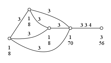
One of the concepts summarizing the properties of an incidence geometry (on which a group acts flag-transitively) is that of a diagram. We provide functionality to compute the diagram of a coset geometry and also to actually draw the diagram. Since a diagram is in fact a labeled graph, drawing is done by producing some code which can be processed by the open source package Graphviz [6]. If the package (which is not a GAP package) is installed on your computer, it will be invoked automatically and the result will be a PostScript file with a picture of the diagram.

⬇

gap> diag:=DiagramOfGeometry(truncation);

gap> DrawDiagram(diag, "truncimg");

gap> Exec("gv␣truncimg.ps");

10.2 Creating the diagram of a coset geometry (see also Example 10.1)

Refer to caption — Figure 1: The diagram of the coset geometry from Example 10.1

Interaction is also provided with the GRAPE package which is very useful in studying a geometry as a (coloured) graph. Using the IncidenceGraph command one obtains the incidence graph of an incidence structure $\mathcal{S}$ . This can then be used, for example, to obtain the full automorphism group of the structure, using the very fast nauty package included with GRAPE. Some shortcut commands have been included for that.

⬇

gap> g := PSL(2,11);;

gap> g1 := Group([ (1,2,3)(4,8,12)(5,10,9)(6,11,7),

(1,2)(3,4)(5,12)(6,11)(7,10)(8,9) ]);;

gap> g2 := Group([ (1,2,7)(3,9,4)(5,11,10)(6,8,12),

(1,2)(3,4)(5,12)(6,11)(7,10)(8,9) ]);;

gap> g3 := Group([ (1,2,11)(3,8,7)(4,9,5)(6,10,12),

(1,2)(3,12)(4,11)(5,10)(6,9)(7,8) ]);;

gap> g4 := Group([ (1,2,11)(3,8,7)(4,9,5)(6,10,12),

(1,2)(3,10)(4,9)(5,8)(6,7)(11,12) ]);;

gap> cg:=CosetGeometry(g,[g1,g2,g3,g4]);

CosetGeometry( Group( [ ( 3,11, 9, 7, 5)( 4,12,10, 8, 6),

( 1, 2, 8)( 3, 7, 9)( 4,10, 5)( 6,12,11) ] ) )

gap> aut:=AutGroupIncidenceStructureWithNauty(cg);

gap> StructureDescription(aut);

"PSL(2,11)"

gap> cor:=CorGroupIncidenceStructureWithNauty(cg);

gap> StructureDescription(cor);

"C2␣x␣PSL(2,11)"

10.3 Incidence geometries and graphs

11 Generalised polygons

A generalised $n$ -gon is a point/line geometry whose incidence graph is bipartite of diameter $n$ and girth $2n$ . Generalised polygons were introduced by J. Tits in [15]. Projective planes are examples of generalised $3$ -gons and classical polar spaces of rank 2 are examples of generalised $4$ -gons, also called generalised quadrangles. Non-classical examples of projective planes and generalised quadrangles are well-known. By the famous theorem of Feit and Higman, a generalised $n$ -gon which has at least three points on every line, must have $n\in\{2,3,4,6,8\}$ . Two classes of examples of generalised hexagons are the so-called split Cayley hexagons and the twisted triality hexagons, which are both derived from a triality of the Lie geometries of type $D_{4}$ , which are in the finite case subgeometries of the hyperbolic quadric $\mathrm{Q}^{+}(7,q)$ . Generalised octagons seem to be rare. In the finite case, only the so-called Ree-Tits octagon (together with its dual) is known. Generalised polygons occur in several ways and one particular generalised polygon can often be represented in different ways. The framework for generalised polygons in FinInG is generic. It provides the user with a set of operations that are always applicable to any generalised polygon (and its elements), independent of its representation. The classical examples such as classical projective planes, classical generalised quadrangles and the classical generalised hexagons are represented as Lie geometries, but are also generalised polygons in FinInG and as such all generic operations for generalised polygons can be used. This generic framework also includes operations that deal with the incidence graph of the generalised polygon.

We give some examples of the different possibilities to construct generalised polygons in FinInG. In Example 11.1 a projective plane of order $4$ is constructed by representing every line as a set of points. The points may be any set of objects, as long as the set of blocks is a set of subsets of the point set. In Example 11.2 the construction of the generalised quadrangle $T_{2}({\mathcal{O}})$ by using elements of a suitable projective space, is demonstrated. Finally, Example 11.3 demonstrates the construction of the Split Cayley hexagon. Note that the construction operations used in the first two examples GeneralisedPolygonByBlocks and GeneralisedPolygonByElements check whether the input really yields a generalised polygon.

⬇

gap> blocks := [

> [ 1, 2, 3, 4, 5 ], [ 1, 6, 7, 8, 9 ], [ 1, 10, 11, 12, 13 ],

> [ 1, 14, 15, 16, 17 ], [ 1, 18, 19, 20, 21 ], [ 2, 6, 10, 14, 18 ],

> [ 2, 7, 11, 15, 19 ], [ 2, 8, 12, 16, 20 ], [ 2, 9, 13, 17, 21 ],

> [ 3, 6, 11, 16, 21 ], [ 3, 7, 10, 17, 20 ], [ 3, 8, 13, 14, 19 ],

> [ 3, 9, 12, 15, 18 ], [ 4, 6, 12, 17, 19 ], [ 4, 7, 13, 16, 18 ],

> [ 4, 8, 10, 15, 21 ], [ 4, 9, 11, 14, 20 ], [ 5, 6, 13, 15, 20 ],

> [ 5, 7, 12, 14, 21 ], [ 5, 8, 11, 17, 18 ], [ 5, 9, 10, 16, 19 ] ];;

gap> gp := GeneralisedPolygonByBlocks( blocks );

11.1 A projective plane constructed by its blocks

⬇

gap> conic := Set(Points(ParabolicQuadric(2,4)));

[ <a point in Q(2, 4)>, <a point in Q(2, 4)>, <a point in Q(2, 4)>,

<a point in Q(2, 4)>, <a point in Q(2, 4)> ]

gap> pg := PG(3,4);

ProjectiveSpace(3, 4)

gap> hyp := HyperplaneByDualCoordinates(pg,[1,0,0,0]*Z(q)^0);

gap> em := NaturalEmbeddingBySubspace(PG(2,4),pg,hyp);

to <All elements of ProjectiveSpace(3, 4)>>

gap> conic_at_infinity := List(conic,x->x^em);;

gap> group := CollineationGroup(pg);

The FinInG collineation group PGammaL(4,4)

gap> stab := FiningSetwiseStabiliser(group,conic_at_infinity);

#I Computing adjusted stabilizer chain...

gap> points1 := Set(Filtered(Points(pg),x->not x in hyp));;

gap> tangents := List(conic,x->TangentSpace(x)^em);

[ <a line in ProjectiveSpace(3, 4)>, <a line in ProjectiveSpace(3, 4)>,

<a line in ProjectiveSpace(3, 4)>, <a line in ProjectiveSpace(3, 4)>,

<a line in ProjectiveSpace(3, 4)> ]

gap> planes := List(tangents,x->Filtered(Planes(x),y->not y in hyp));;

gap> points2 := Union(planes);;

gap> points3 := [hyp];

[ <a plane in ProjectiveSpace(3, 4)> ]

gap> linesa := Union(List(conic_at_infinity,x->Filtered(Lines(x),y->not y in hyp)));;

gap> linesb := Set(conic_at_infinity);;

gap> pts := Union(points1,points2,points3);;

gap> lns := Union(linesa,linesb);;

gap> inc := \*;

gap> gp := GeneralisedPolygonByElements(pts,lns,inc,stab,\^);

11.2 A generalised quadrangle

T_{2}(O)

⬇

gap> gp := SplitCayleyHexagon(3);

H(3)

11.3 A classical generalised hexagon

Example 11.4 shows some particular operations on (the elements of) generalised polygons. We use the Ree-Tits octagon as example. Note that the construction of this octagon is done by GeneralisedPolygonByElements based on the construction as a coset geometry, also demonstrating that the construction operations for generalised polygons are generic.

⬇

gap> LoadPackage( "AtlasRep" );

true

gap> titsgroup:=AtlasGroup("2F4(2)’");

gap> g1:=AtlasSubgroup(titsgroup,3);

gap> g2:=AtlasSubgroup(titsgroup,5);

gap> conj:=ConjugacyClassSubgroups(titsgroup,g1);;

gap> # Now look for the conjugate of g1 with maximal intersection

gap> g1:=First(conj, sg -> Size(Intersection(sg,g2))=2048);

gap> cg:=CosetGeometry(titsgroup,[g1,g2]);;

gap> pts := Set(ElementsOfIncidenceStructure(cg,1));;

gap> lines := Set(ElementsOfIncidenceStructure(cg,2));;

gap> gp := GeneralisedPolygonByElements(pts,lines,\*,titsgroup,OnCosetGeometryElement);

gap> Order(gp);

[ 2, 4 ]

gap> p := Random(Points(gp));

gap> lines := Lines(p);

gap> l := Random(lines);

gap> DistanceBetweenElements(p,l);

gap> m := Random(Lines(gp));

gap> DistanceBetweenElements(m,l);

11.4 The Ree-Tits octagon from a coset geometry

The third example shows these particular examples on the classical generalised polygons.

⬇

gap> h := TwistedTrialityHexagon(2^3);

T(8, 2)

gap> p := Random(Points(h));

#I Computing nice monomorphism...

#I Found permutation domain...

gap> lines := Lines(p);

gap> l := Random(lines);

gap> DistanceBetweenElements(p,l);

gap> m := Random(Lines(h));

gap> DistanceBetweenElements(m,l);

11.5 Elements of the twisted triality hexagon

12 Algebraic varieties

In FinInG some basic functionality for algebraic varieties defined over finite fields is implemented. The algebraic varieties in FinInG are defined by a list of multivariate polynomials over a finite field, and an ambient geometry. This ambient geometry is either a projective space, in which case the algebraic variety is called a projective variety, or an affine geometry, in which case the algebraic variety is called an affine variety. There is an iterator for the set of points that lie on the variety and the user is enabled to randomly choose one of these points.

⬇

gap> r:=PolynomialRing(GF(5),6);

GF(5)[x_1,x_2,x_3,x_4,x_5,x_6]

gap> f1:=Sum(List(IndeterminatesOfPolynomialRing(r),x->x^2));

x_1^2+x_2^2+x_3^2+x_4^2+x_5^2+x_6^2

gap> f2:=r.1*r.2+r.3*r.4+r.5*r.6;

x_1*x_2+x_3*x_4+x_5*x_6

gap> var:=AlgebraicVariety(PG(5,5),[f1,f2]);

Projective Variety in ProjectiveSpace(5, 5)

gap> Points(var);

gap> Size(Points(var));

156

gap> Random(Points(var));

12.1 Constructing an algebraic variety

Specific methods are available for Hermitian varieties and quadrics, as well as a method PolarSpace which returns the associated polar space consistent with the other functionality for polar spaces defined from forms.

⬇

gap> hv:=HermitianVariety(3,9);

Hermitian Variety in ProjectiveSpace(3, 9)

gap> hp:=PolarSpace(hv);

gap> DefiningListOfPolynomials(hv);

[ x_1^4+x_2^4+x_3^4+x_4^4 ]

gap> hv:=HermitianVariety(3,9);

Hermitian Variety in ProjectiveSpace(3, 9)

gap> DefiningListOfPolynomials(hv);

[ x_1^4+x_2^4+x_3^4+x_4^4 ]

gap> hp:=PolarSpace(hv);

gap> PolarSpaceType(hp);

"hermitian"

gap> IsGeneralisedQuadrangle(hp);

true

gap> Order(hp);

[ 9, 3 ]

12.2 A Hermitian variety

The package FinInG also contains the Veronese varieties, the Segre varieties and the Grassmann varieties; three classical projective varieties. These varieties have an associated geometry morphism (VeroneseMap, SegreMap, and GrassmannMap) and FinInG also provides some general functionality for these. Example 12.3 shows this for the Veronese variety in a five-dimensional projective space, by constructing the set of planes intersecting the variety in a conic.

⬇

gap> vv:=VeroneseVariety(PG(2,3));

Veronese Variety in ProjectiveSpace(5, 3)

gap> DefiningListOfPolynomials(vv);

[ -x_1*x_4+x_2^2, -x_1*x_6+x_3^2, -x_4*x_6+x_5^2, x_1*x_5-x_2*x_3 ]

gap> vm:=VeroneseMap(vv);

Veronese Map of <points of ProjectiveSpace(2, 3)>

gap> Range(vm);

gap> vvpts:=Set(Points(vv));;

gap> linesets:=List(Lines(PG(2,3)),l->List(Points(l)));;

gap> image_list:=List(linesets,list->Span(ImagesSet(vm,list)));

[ <a plane in ProjectiveSpace(5, 3)>, <a plane in ProjectiveSpace(5, 3)>,

<a plane in ProjectiveSpace(5, 3)>, <a plane in ProjectiveSpace(5, 3)>,

<a plane in ProjectiveSpace(5, 3)> ]

gap> List(image_list,plane->Number(Points(plane),x->x in vvpts));

[ 4, 4, 4, 4, 4, 4, 4, 4, 4, 4, 4, 4, 4 ]

gap> vvstab:=FiningSetwiseStabiliser(HomographyGroup(PG(5,3)),vvpts);

#I Computing adjusted stabilizer chain...

gap> plane_orbs:=FiningOrbits(vvstab,Planes(PG(5,3)));

1%..3%..4%..5%..6%..7%..12%..14%..23%..28%..29%..38%..39%..

43%..52%..60%..61%..63%..66%..68%..77%..82%..90%..99%..

100%..[ <closed orbit, 13 points>, <closed orbit, 13 points>,

<closed orbit, 104 points>, <closed orbit, 468 points>,

<closed orbit, 468 points>, <closed orbit, 468 points>,

<closed orbit, 468 points>, <closed orbit, 234 points>,

<closed orbit, 468 points>, <closed orbit, 1404 points>,

<closed orbit, 936 points>, <closed orbit, 2808 points>,

<closed orbit, 1872 points>, <closed orbit, 351 points>,

<closed orbit, 2808 points>, <closed orbit, 234 points>,

<closed orbit, 351 points>, <closed orbit, 1404 points>,

<closed orbit, 2808 points>, <closed orbit, 2808 points>,

<closed orbit, 468 points>, <closed orbit, 702 points>,

<closed orbit, 936 points>, <closed orbit, 702 points>,

<closed orbit, 2808 points>, <closed orbit, 1872 points>,

<closed orbit, 2808 points>, <closed orbit, 2808 points>,

<closed orbit, 144 points>, <closed orbit, 144 points> ]

gap> Filtered(plane_orbs,o->Number(Points(o[1]),x->x in vvpts)=4);

[ <closed orbit, 13 points> ]

gap> conicplanes:=last[1];

gap> ForAll(image_list,plane->plane in conicplanes);

true

12.3 A Veronese variety

References

[1] J. Bamberg, A. Betten, P. Cara, J. De Beule, M. Lavrauw, and M. Neunhöffer, FinInG – Finite Incidence Geometry, Version 1.3.3, 2016.
[2] J. Bamberg and J. De Beule, FORMS – Sesquilinear and Quadratic, Version 1.2.2, 2011.
[3] W. Bosma, J. Cannon, and C. Playoust, The Magma algebra system. I. The user language, J. Symbolic Comput., 24 (1997), pp. 235–265. Computational algebra and number theory (London, 1993).
[4] F. Buekenhout and A. M. Cohen, Diagram geometry, vol. 57 of Ergebnisse der Mathematik und ihrer Grenzgebiete. 3. Folge. A Series of Modern Surveys in Mathematics [Results in Mathematics and Related Areas. 3rd Series. A Series of Modern Surveys in Mathematics], Springer, Heidelberg, 2013. Related to classical groups and buildings.
[5] S. De Winter and J. Schillewaert, Characterizations of finite classical polar spaces by intersection numbers with hyperplanes and spaces of codimension 2, Combinatorica, 30 (2010), pp. 25–45.
[6] E. R. Gansner and S. C. North, An open graph visualization system and its applications to software engineering, SOFTWARE - PRACTICE AND EXPERIENCE, 30 (2000), pp. 1203–1233.
[7] The GAP Group, GAP – Groups, Algorithms, and Programming, Version 4.7.5, 2014.
[8] P. Kleidman and M. Liebeck, The subgroup structure of the finite classical groups, vol. 129 of London Mathematical Society Lecture Note Series, Cambridge University Press, Cambridge, 1990.
[9] M. Lavrauw and G. Van de Voorde, Field reduction and linear sets in finite projective geometry, in Topics in Finite Fields, G. Kyureghyan, G. Mullen, and A. Pott, eds., vol. 632, AMS Contemporary Math., 2015, pp. 271–293.
[10] J. Müller, M. Neunhöffer, and F. Noeske, orb – Methods to enumerate Orbits, Version 4.7.1, 2014.
[11] M. Neunhöffer, cvec – Compact vectors over finite fields, Version 2.4, 2014.
[12] M. Neunhöffer and F. Noeske, genss – Generic Schreier-Sims, Version 1.6.2, 2014.
[13] L. Soicher, DESIGN – The Design Package for GAP, Version 1.6, 2011.
[14] , GRAPE – GRaph Algorithms using PErmutation groups, Version 4.6.1, 2012.
[15] J. Tits, Sur la trialité et certains groupes qui s’en déduisent, Inst. Hautes Études Sci. Publ. Math., (1959), pp. 13–60.