Compact Stars in Vector-Tensor-Horndeski Theory of Gravity

Abstract

In this paper, we will analyse a theory of modified gravity, in which the field content of general relativity will be increased to include a vector field. We will use the Horndeski formalism to non-minimally couple this vector field to the metric. As we will be using the Horndeski formalism, this theory will not contain Ostrogradsky ghost degree of freedom. We will analyse compact stars using this Vector-Tensor-Horndeski theory.

1 Introduction

Even though general relativity is a very well-tested theory, there is a strong motivation to modify general relativity at large scale. This is because to explain the accelerating cosmic expansion in general relativity, a cosmological constant has to be included [1, 2, 3, 4, 5, 6] . Even though the existence of such a cosmological constant is predicted from quantum field theories, quantum field theories predict a cosmological constant which is $10^{120}$ times larger than the observed value of the cosmological constant. This has motivated the study of modified theories of gravity, and the Scalar-Tensor theories are such a modification of general relativity which could explain accelerating cosmic expansion [7, 8]. However, these theories in general contain higher derivative terms in the action, and such higher derivative terms gives rise to Ostrogradsky ghost degree of freedom. These in turn cause instabilities in the theory called the Ostrogradsky instabilities. It is possible to avoid Ostrogradsky ghosts by using a theory with galileon symmetry [9, 10, 11, 12]. Even though this galileon theory also contains higher derivative terms in the action, the galilean symmetry ensures that the field equations are only second-order differential equations. Thus, the galilean symmetry ensures that the Ostrogradski ghost instabilities are avoided in these theories. In the decoupling limit, this theory contains a higher-order derivative interaction known as the cubic galileon. It is possible to construct a theory with quartic and quintic Galileon [13]. It is necessary to add couplings of the scalar to curvature tensors, away from the decoupling limit. This way the Horndeski theory is obtained, and field equations for both the scalar field and the metric are again second order differential equations [14, 15]. So, Horndeski theory is also free from Ostrogradsky ghosts, and it does not contain the Ostrogradsky instabilities associated with these ghosts.

This Horndeski formalism is a general formalism and it can be used to analyse a non-minimal coupling of other fields to the metric. Thus, it is possible to analyse a Horndeski coupling of the metric to a vector field [16, 17]. In this formalism, the vector field is again coupled to the metric using a non-minimal coupling. Furthermore, the field equations for this vector field are again second-order field equations. Thus, the Ostrogradsky ghost terms are avoided even for the Horndeski coupling of a vector field to the metric. As we will be interested in applying such a Vector-Tensor-Horndeski theory to astrophysics, we will assume such a vector field is a fundamental field in nature, which is obtained by increasing the field content of general relativity, and it is not the usual electromagnetic field. This is important as astrophysical objects are neutral and do not have an electric charge. So, the electromagnetic field cannot have a direct effect on the physics of such astrophysical objects. Furthermore, it is known that the gravity couples to the electromagnetic field in the usual way, and there is no reason for it to couple to the physical electromagnetic field in a non-minimal way in any astrophysical object. However, if we assume that there exists an astrophysical vector field, which has negligible effect on small scale, then it is possible that such an astrophysical vector field can couple to the metric in a non-minimal way. This coupling of such an astrophysical vector field can have non-trivial effects on the astrophysical phenomena. So, in this paper, we will analyse the effect of such a non-minimal coupling of an astrophysical vector field on the physics of a compact star.

It may be noted that such fundamental vector fields have been proposed as a solution to various different physical problems, and have also been used to explain many interesting astrophysical phenomena. Just like the scalar fields, the vector field have also been used to explain cosmic expansion [23, 24], and even the naturalness problem [25, 26]. It may be noted that there the Vector-Tensor theories produce many non-trivial phenomenological effects which can not be produced in the Scalar-Tensor theories [27, 28, 29, 30]. It has been observed that anomalies exist in the alignment of the low multipoles of the CMB [18, 19] and the hemispherical asymmetry [20]. Such anomalies suggest that there might be a preferential direction in the universe, and this can be explained using such a vector field. Furthermore, such fundamental vector fields have also been used to study inflation [21, 22]. The occurrence of higher derivative terms can produce Ostrogradski ghost instability in such Vector-Tensor theories. However, such Ostrogradski ghost instability can be avoided by using the Horndeski formalism. Thus, it is interesting to study a Vector-Tensor-Horndeski theory. It may be noted that there are other interesting motivation to introduce such vector fields. This is because there exists a discrepancy between the predicted and observed dynamics of galaxies  [31, 32, 33], and it has been proposed that the discrepancy can be resolved by increasing the field content of general relativity [36, 37, 38, 39, 40, 41]. The field content of this modified theory of gravity contains such a vector field. It may be noted that this theory agrees with the predictions made by the modified newtonian dynamics [34, 35].

As the field content of general relativity contains a vector field, it has been observed that astrophysical black holes in this modification of gravity can mathematically resemble a Reissner–Nordstrom solution  [42, 43]. However, the charge of this vector field is generated from mass and not an electromagnetic source [42, 43]. As the astrophysical objects are not charged, and so any coupling of metric to a electromagnetic field cannot be applied to study such astrophysical objects. However, as this additional vector field is produced from mass and not electric charge [42, 43], it is possible that such a field can have direct effect on astrophysical phenomena. Furthermore, in this theory, there is a certain amount of freedom to choose the action for vector field, and it has been demonstrated that coupling the metric to a non-linear vector field can turn a black hole into a gray hole [44]. As it has been demonstrated that different form of the vector field action can produce different physical results, it is interesting to investigate other forms of coupling of vector field to metric. Furthermore, as this vector field occur in the field content of general relativity, it will also be interesting to investigate the astrophysical application of such a theory. So, in this paper, we will use the Horndeski formalism to couple a vector field to the metric, and we use this Vector-Tensor-Horndeski theory to analyse a compact star.

2 Vector-Tensor-Horndeski Theory

In this section, we will analyse the main features of a Vector-Tensor-Horndeski theory. It has been proposed that by increasing the field content of general relativity certain astrophysical phenomena can be explained [36, 37, 38, 39, 40, 41]. Furthermore, for compact stars this would deform astrophysical solutions, and these deformed solutions would resemble a charged black hole solution [42, 43]. It is physically important to point out that the vector field introduced here is not the usual electromagnetic field, but an astrophysical vector field and it has negligible effect at small scale. However, it is expected to change the astrophysical dynamics at larger scale. In this section, we will use the Horndeski formalism to non-minimally couple such a vector field to the metric. Thus, we first introduce as astrophysical vector field $A_{\mu}$ with the field tensor $F_{\mu\nu}=\nabla_{\nu}A_{\mu}-\nabla_{\mu}A_{\nu}$. We denote the source for such a vector field as $J^{\nu}$ . Now the energy-momentum tensor for this astrophysical vector field can be written as $T_{\mu\nu}=\frac{1}{4\pi}\Big{(}F_{\mu}^{\alpha}F_{\nu\alpha}-\frac{1}{4}g_{\mu\nu}F^{\alpha\beta}F_{\alpha\beta}\Big{)}$, and we will also denote the energy-momentum tensor for other fields in the theory by $T_{\mu\nu}^{M}$ . There is a conserved charge associated with this vector field, as we can write a divergence free current $\nabla_{\nu}J^{\nu}=0$. Now using Horndeski formalism [16, 17], we couple this astrophysical vector field to the metric as

$$G_{\mu\nu}=8\pi G(T_{\mu\nu}+\kappa U_{\mu\nu}+T_{\mu\nu}^{M}),$$

$$\nabla_{\mu}F^{\mu\nu}+\frac{\kappa}{2}\nabla_{\alpha}F_{\beta\gamma}\mathcal{R}^{\nu\alpha\beta\gamma}=4\pi J^{\nu}.$$ (1)

where $U^{\mu\nu}$ is given by

$$U^{\mu\nu}=\frac{1}{8\pi}\Big{(}F_{\alpha\beta}F^{\beta}_{\gamma}\mathcal{R}^{\mu\alpha\nu\gamma}+\nabla^{\beta}\mathcal{F}^{\mu\alpha}\nabla_{\alpha}\mathcal{F}^{\nu}_{\beta}\Big{)}$$ (2)

It may be noted that if $\kappa=0$, this theory reduced to the usual Vector-Tensor theory. However, we would like to analyse this modified Vector-Tensor-Horndeski theory. The dual tensors can be defined as $\mathcal{R}^{\alpha\beta}_{\mu\nu}=\eta^{\alpha\beta\gamma\delta}\eta_{\mu\nu\epsilon\zeta}R^{\epsilon\zeta}_{\gamma\delta}/4$ and $\mathcal{F}^{\alpha\beta}=\eta^{\alpha\beta\gamma\delta}F_{\gamma\delta}/2$, where $\eta^{\alpha\beta}_{\gamma\delta}=\delta^{[\alpha\beta]}_{[\gamma\delta]}/4!$ is total asymmetric Levi-Civita tensor. Thus, we can write the Lagrangian for this Vector-Tensor-Horndeski theory as

$$\mathcal{L}=-\frac{R}{16\pi G}+F^{\alpha\beta}F_{\alpha\beta}+\frac{\kappa}{2}F_{\alpha\beta}F^{\gamma\delta}\mathcal{R}^{\alpha\beta}_{\gamma\delta}.$$ (3)

This Lagrangian has a non-trivial coupling between the astrophysical vector field and the metric, which was not present in other Vector-Tensor theories of gravity [36, 37, 38, 39, 40, 41] .

The static spherically symmetric solutions for a vector field has been studied using the Horndeski formalism [16, 17]. We will apply this solution to analyse a compact star in this theory, because even though physically, this vector field is an astrophysical vector field, mathematically, this solution will resemble the static spherically symmetric solutions for a Horndeski vector field [16, 17]. However, unlike the electromagnetic fields which cannot have a direct effect on compact stars, this vector field can change the behavior of compact stars. Now for this Horndeski astrophysical vector field $A_{\mu}$ , we have $J_{\mu}dx^{\mu}=j(r)dr$, and for isotropic matter fields, we can take a perfect fluid with $T^{\mu(M)}_{\nu}=\big{(}\rho,-p-p,-p\big{)}$. The static spherically symmetric metric for a compact star can be written in the Schwarzschild-Droste coordinates $x^{\mu}=(t,r,\varphi,\theta)$. Furthermore, for this astrophysical vector field, we write $F_{\mu\nu}dx^{\mu}\otimes dx^{\nu}=f(r)g_{tt}g_{rr}(dt\otimes dr-dr\otimes dt)$. Here we choose the units, such that $c=1$. Now the metric for this solution can be written as

$$ds^{2}=e^{2\psi(r)}dt\otimes dt-e^{2\phi(r)}dr\otimes dr-r^{2}d\theta\otimes d\theta-r^{2}\sin^{2}\theta d\varphi\otimes d\varphi.$$ (4)

The equation of motion for this solution can be written as

$$e^{-2\phi}\Big{(}\frac{2\phi^{\prime}}{r}+\frac{e^{2\phi}-1}{r^{2}}\Big{)}=f^{2}+\frac{\kappa f^{2}}{r^{2}}(e^{-2\phi}-1)+8\pi G\rho,$$ (5)

$$e^{-2\phi}\Big{(}\frac{2\psi^{\prime}}{r}+\frac{1-e^{2\phi}}{r^{2}}\Big{)}=-f^{2}-\frac{\kappa f^{2}}{r^{2}}(3e^{-2\phi}-1)+8\pi Gp$$ (6)

$$e^{-2\phi}\Big{(}\psi^{\prime\prime}-\phi^{\prime}\psi^{\prime}+\psi^{\prime 2}+\frac{\psi^{\prime}-\phi^{\prime}}{r}\Big{)}=f^{2}+8\pi Gp$$

$$+\frac{\kappa fe^{-2\phi}}{r}\big{(}f(\phi^{\prime}-\psi^{\prime})-2f^{\prime}\big{)}$$ (7)

$$f^{\prime}+\frac{2f}{r}-\frac{\kappa}{r^{2}}\big{(}f^{\prime}(1-e^{-2\phi})+2f\phi^{\prime}e^{-2\phi}\big{)}=4\pi j(r),$$ (8)

We can write the hydrostatic equation for matter sector as$\nabla_{\mu}T^{\mu(M)}_{\nu}=0$ for $\nu=r$ , and thus we obtain $p^{\prime}+\psi^{\prime}(p+\rho)=0.$ Now we can write Eqs. (5-2) in terms of thermodynamic parameters, and this can be done by redefine the metric function $\phi$ in terms of a mass function $M(r)$ as

$$e^{-2\phi}=1-\frac{2GM}{r}.$$ (9)

So, we can obtain the differential change in mass $dM$, which is the mass stored in a layer with thickness $dr$ as

$$\frac{GdM}{dr}=\frac{1}{2}\Big{[}1-e^{-2\phi}(1-2r\phi^{\prime})\Big{]},$$ (10)

where $M$ is the mass of the compact object. Now make the equations dimensionless by expressed them in terms of $\{\frac{dp}{dr},\frac{dM}{dr},\rho,p\}$, and by using $M\to mM_{\odot}$, $r\to r_{g}r$, $\rho\to\rho M_{\odot}/r_{g}^{3}$, $p\to pM_{\odot}/r_{g}^{3}$ and $R\to R/r_{g}^{2}$. Here $r_{g}=G_{N}M_{\odot}=1.47473\mbox{km}$ , $M_{\odot}$ is the mass of the Sun, and

$$\frac{d\phi}{dr}=\frac{m}{r^{2}}\frac{1-\frac{r}{m}\frac{dm}{dr}}{\frac{2m}{r}-1}.$$ (11)

Thus, we obtain

$$\frac{2m}{r^{3}}(1-\frac{r}{m}\frac{dm}{dr})-\frac{2m}{r^{3}}+r_{g}^{2}f^{2}-\frac{2m\kappa f^{2}}{r^{3}}=8\pi\rho,$$ (12)

$$\frac{2p^{\prime}}{r(p+\rho)}(1-\frac{2m}{r})+\frac{2m}{r^{3}}-r_{g}^{2}f^{2}-\frac{2\kappa f^{2}}{r^{2}}(1-\frac{3m}{r})=8\pi p$$ (13)

$$\Big{(}\frac{p^{\prime}}{p+\rho}\Big{)}^{\prime}-\frac{m}{r^{2}}\frac{1-\frac{r}{m}\frac{dm}{dr}}{\frac{2m}{r}-1}\frac{p^{\prime}}{p+\rho}-\Big{(}\frac{p^{\prime}}{p+\rho}\Big{)}^{2}+\frac{p^{\prime}}{r(p+\rho)}$$

$$+\frac{m}{r^{3}}\frac{1-\frac{r}{m}\frac{dm}{dr}}{\frac{2m}{r}-1}+\frac{f^{2}r_{g}^{2}}{1-\frac{2m}{r}}$$ (14)

$$+\frac{\kappa f}{r}\big{(}f(\frac{m}{r^{2}}\frac{1-\frac{r}{m}\frac{dm}{dr}}{\frac{2m}{r}-1}+\frac{p^{\prime}}{p+\rho})-2f^{\prime}\big{)}=\frac{8\pi p}{1-\frac{2m}{r}}$$

$$f^{\prime}+\frac{2f}{r}-\frac{\kappa r_{g}^{-2}}{r^{2}}\big{(}\frac{2mf^{\prime}}{r}-\frac{2mf}{r^{2}}(1-\frac{r}{m}\frac{dm}{dr})\big{)}=4\pi r_{g}j(r),$$ (15)

We will analyse a compact start by solving Eqs. (12-15). Furthermore, we will also use the equation of state $p=p(\rho)$ and a specific form of $j(r)$ to obtain such solutions. The function $m(r)$ is important in analyzing the geometric mass inside a sphere of radius $r$. This is because we can use Eq. (10) , and write

$$m^{\prime}(r)=\frac{1}{2}\Big{[}r(1-e^{-2\phi})\Big{]}^{\prime}.$$ (16)

Furthermore, from Eq. (5), we obtain

$$m^{\prime}(r)=4\pi r^{2}\rho-r^{2}f^{2}\Big{[}1+\frac{\kappa}{r^{2}}(e^{-2\phi}-1)\Big{]}.$$ (17)

It may be noted in the absence of the Horndeski field, $f=0$, the Eq. (17) reduces to the usual form $m^{\prime}(r)=4\pi r^{2}\rho$ in general relativity. Now by integrating Eq. (17), we obtain

$$m(R)\equiv M=\int_{0}^{R}\Big{(}4\pi r^{2}\rho-r^{2}f^{2}\Big{[}1+\frac{\kappa}{r^{2}}(e^{-2\phi}-1)\Big{]}\Big{)}dr.$$ (18)

Now using this result, we can obtain

$$\frac{2p^{\prime}}{r(p+\rho)}(1-\frac{2m}{r})+\frac{2m}{r^{3}}+\Big{[}\frac{8\pi\rho+\frac{2m}{r^{3}}(1-\frac{r}{m}\frac{dm}{dr})-\frac{2m}{r^{3}}}{r_{g}^{2}-\frac{2m\kappa}{r^{3}}}\Big{]}$$

$$\Big{(}r_{g}^{2}+\frac{2\kappa}{r^{2}}(1-\frac{3m}{r})\Big{)}=8\pi p$$ (19)

Now the equation of state for this system can be written as $p=p(\rho)$, It is possible to integrate this equation of state to obtain the behavior of this system in this Vector-Tensor-Horndeski theory. The boundary conditions used for analyzing this system in this Vector-Tensor-Horndeski theory are similar to those used in the Einstein gravity, $m(0)=0,\rho(0)=\rho_{c},$ and $p(r_{0})=0$. So, the radius of the compact star can be taken to be $r_{0}$ , such that the pressure vanishes. Now we can analyse compact stars using this formalism. In astrophysics, the term compact star is used to collectively refer to white dwarfs, neutron stars, and black holes. They are described by Tolman-Oppenheimer-Volkoff equations [45, 46]. In this section, we will analyse the effect of the Horndeski astrophysical vector field on the physics of such compact stars.

3 The Gravitational Binding Energy

The gravitational binding energy of a system is the minimum energy that must be added to that system for it to stop being a a gravitationally bound system. It is important to analyze the gravitational binding energy of compact stars, such as the neutron star, and such an analysis has been done using general relativity [47, 48, 49]. So, in this section, we shall analyze the effect of the astrophysical Horndeski field on the gravitational binding energy of a compact star. Thus, using the definition of the mass function (18), the total mass of the matter distribution of this system can be represented by

$$m_{ADM}=4\pi\int_{o}^{\infty}dr\rho(r)r^{2}+\Delta m_{ADM}.$$ (20)

This mass is the Arnowitt-Deser-Misner (ADM) mass and in the Horndeski-Vector-Tensor theory. It may be noted that $\Delta m_{ADM}$ is the corrections to the usual ADM mass produced by the the Horndeski vector field,

$$\Delta m_{ADM}=-\int_{0}^{\infty}\Big{(}r^{2}f^{2}\Big{[}1+\frac{\kappa}{r^{2}}(e^{-2\phi}-1)\Big{]}\Big{)}dr.$$ (21)

Now we can define the density inside a proper volume element $\sqrt{-g}d^{3}x$ as the proper mass,

$$M_{pr}=4\pi\int_{0}^{\infty}dr\rho(r)e^{\phi(r)}r^{2}$$ (22)

We interpret the difference between the proper (22) and the total mass (18) as the gravitational binding energy

$$E_{b}=M_{pr}-m>0.$$ (23)

In general relativity, due to the absence of vector or Horndeski fields, $f=0$ and $\Delta m_{ADM}=0$. However, as we have a non-minimal coupling to the Horndeski field, the ADM mass is corrected by a finite $\Delta m_{ADM}\neq 0$.

To analyze the effect of the astrophysical vector field on compact stars, we need to solve the modified Tolman-Oppenheimer-Volkoff equation, Eq. (2). However, to solve this equation, we need to use the equation of state for the interior structure of the star. It is possible to write this equation of state using the central density, $\rho(r=0)=\rho_{c}$, as a free parameter. Thus, we can obtain the mass and radius of a star by fixing the central density. This will correspond to choosing a single point in the mass-radius diagram for the star. As this system is described by a single parameter, we can obtain the full mass-radius curve of the star by varying $\rho_{c}$. It is possible to study the inner structure of the compact stars, such as the neutron stars [50]. This is because it possible to use microscopic many-body simulations to numerically analyze equation of state for such compact stars. The equation of state for compact stars can be obtained using a mean-field theoretical description of such a system [51, 52, 53]. In fact, it is possible to describe the equation of state for a neutron star using the nucleon-nucleon interaction. The equation of state for such a star is is a polytrope equation of state [50],

$$p=k\rho^{\gamma}$$ (24)

The value of $k$ can be taken to be $k\approx 2.0\times 10^{5}\frac{cm^{5}}{gs2}$ when $\gamma=2$ [54]. We can now use this polytrope equation of state to analyze the effect of Horndeski field on a neutron star.

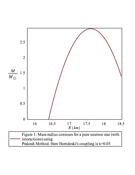
Figure 1: Mass-radius contours for a pure neutron star (with interactions) using Prakash Method. Here Horndeski’s coupling is $\kappa=0.05$

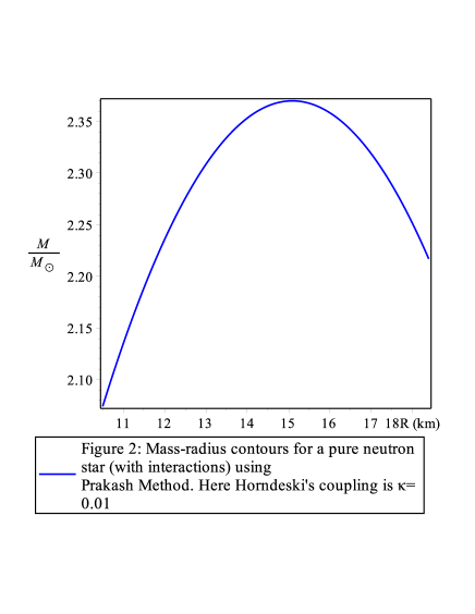
Figure 2: Mass-radius contours for a pure neutron star (with interactions) using Prakash Method. Here Horndeski’s coupling is $\kappa=0.01$

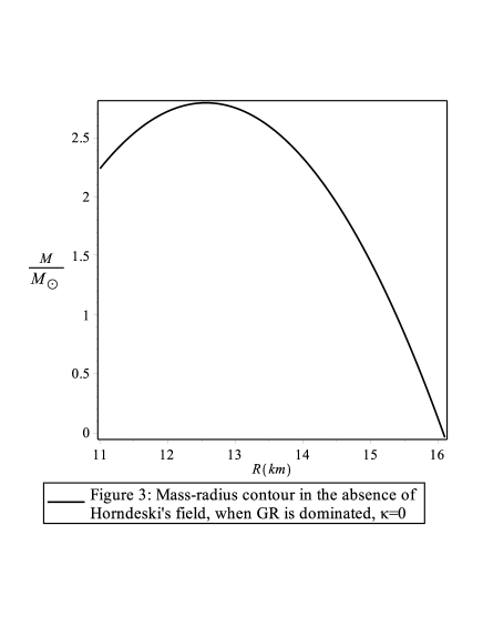
Figure 3: Mass-radius contour in the absence of Horndeski’s field, when general relativity is dominated, $\kappa=0$.

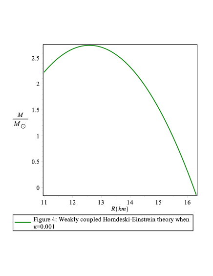
Figure 4: Mass-radius contour when Horndeski’s field is weakly coupled, $\kappa=0.001$.

We have used an adaptive step-size Runge-Kutta method for analyzing a non-linear-integro-differential equation [55],[56]. This is because the modified Tolman-Oppenheimer-Volkoff equation is a non-linear-integro-differential equation. In Figure. (2), blue line represents the Vector-Tensor-Horndeski theory for $\kappa=0.01$. It predicts the existence of a typical neutron star with mass around $2M_{\odot}$, and a radius around $10-15Km$. Thus, this case is not physical. In fact, this case can also be used to set a bound on the strength of the coupling of this astrophysical vector field to general relativity. In Figure. (3), the black line represents the standard general relativity, $\kappa=0$. The mass-radius diagram corresponding to this case is given in Fig. (1)-(4). In Fig. (1), the red line represents the Vector-Tensor-Horndeski theory with $\kappa=0.05$. It does not predict the existence of a typical neutron star with mass around $2M_{\odot}$, and with a radius around $10-15Km$. It may be noted that for $\kappa<0$, the numerical evaluation does not converge. Furthermore, a stable stellar configurations does not exist for this case, as the hydrostatic equilibrium equations are unstable. The mass-radius profile for a weakly coupled Vector-Tensor-Horndeski theory ($\kappa=10^{-3}$) is plotted in Fig. (4). We observed that this profile around the maximum with mass is similar to the profile obtained in the general relativity. However, for large radius, equilibrium configurations in the Vector-Tensor-Horndeski theory are more massive than in general relativity.

4 Density Profile

It is possible to analyze a compact star to be represented by a constant density. It may be noted that the compact stars with constant density have been analysed in general relativity [59] (see [60] for a comprehensive review). In general relativity the Tolman-Oppenheimer-Volkoff equation admits an analytical solution, and this is obtained by imposing $p(r=r_{0})=0$. Here the central pressure $p_{c}=p(r=0)$ predicted by general relativity becomes infinite for the critical mass $M_{cr}=4/9m_{pl}^{2}r_{0}$ [57]. So, it is possible for stars with $M>M_{cr}$ to indicate a deviation from general relativity [58]. Thus, it is interesting to analyze the effect of a Horndeski vector field for such a system. We can first analyse a uniform mass density called as top-hat density profile inside the star,

$$\rho=\cases{\rho_{{0}}&$r<r_{{0}}$\cr 0&$r_{{0}}\leq r$\cr}$$ (25)

Here we shall now analyse such a system using modified Vector-Tensor-Horndeski theory. Now for this model and for simplicity, we also choose $j(r)=0$. So, the unknown functions for this system are $\{m(r),f(r)\}$, and the metric function is $\psi=\psi_{0}$. Exact solution for the Vector-Tensor-Horndeski theory, for this system can be written as

$$m(r)=\frac{4}{3}\,\pi\,\rho\,{r}^{3}+\,{\frac{2\pi\,\rho\,{r_{{g}}}^{2}{r}^{5}}{15\kappa}}+O\left({r}^{6}\right)$$ (26)

Now using (26) and Eq. (9), we obtain

$$\phi\left(r\right)=-\frac{1}{2}\ln\left(1+\frac{8}{3}\,\pi\,\rho\,{r}^{2}-{\frac{4}{15}}\,{\frac{\pi\,\rho\,{r}^{4}{{r_{g}}}^{2}}{\kappa}}+O\left({r}^{5}\right)\right)$$ (27)

The metric of this compact star can be written as

$$ds^{2} = e^{2\psi_{0}}dt\otimes dt-r^{2}d\theta\otimes d\theta-r^{2}\sin^{2}\theta d\varphi\otimes d\varphi$$ (28)

$$-\frac{dr\otimes dr}{1+\frac{8}{3}\,\pi\,\rho\,{r}^{2}-{\frac{4}{15}}\,{\frac{\pi\,\rho\,{r}^{4}{{\it rg}}^{2}}{\kappa}}+O\left({r}^{5}\right)}.$$

Now using this mass profile, we can integrate Eq, (15), and obtain

$$f\left(r\right)=f_{{0}}+O\left(\left(r-R\right)^{2}\right)$$ (29)

$$+{\frac{\left(30\,f_{{0}}{r_{{g}}}^{2}-80\,\pi\,\rho\,f_{{0}}\kappa-16\,\pi\,\rho\,f_{{0}}{r_{{g}}}^{2}{R}^{2}\right)\left(r-R\right)}{-15\,R{r_{{g}}}^{2}+40\,\pi\,\rho\,R\kappa+4\,\pi\,\rho\,{R}^{3}{r_{{g}}}^{2}}}$$

Here we have assumed that this astrophysical vector field satisfies the following initial condition on the surface of star $r=R$, $f(R)=f_{0}.$ As the original function is corrected by a $\kappa$ dependent terms, it can be argued that such corrections are produced by the Horndeski vector field. As such a coupling between gravity and Horndeski vector field is constraint by experimental data, it is possible to use the astrophysical data to constraint such a coupling.

We analyzed a compact star with a constant density. However, for real stars, we expect that the density to be a function of $r$. So, it is interesting to analyse various different functional dependence of $m(r)$, and analyse the effect of Horndeski vector field on a system described by such functions. This is important to demonstrate that the dependence of the system on Horndeski vector field is not a special feature of a system with a constant density. Now we can take a simple function $m(r)$ of $r$, such as $m(r)=M_{0}\ln(r)$, to demonstrate that the Horndeski vector field effects the systems in which the density is not a constant. Now for such a system, we obtain

$$f(r)=f_{{0}}+O((r-R)^{2})+\,{\frac{2f_{{0}}({R}^{3}{r_{{g}}}^{2}+\kappa\,M_{{0}}\ln(R)-\kappa\,M_{{0}})(r-R)}{R(-{R}^{3}{r_{{g}}}^{2}+2\,\kappa\,M_{{0}}\ln(R))}}$$ (30)

The mass density of this system can be obtained from Eq. (12), and it is given by

$$\rho(r)=\,{\frac{{f_{{0}}}^{2}\Sigma(-{r_{{g}}}^{2}{r}^{3}+2\,m\kappa)}{8{r}^{3}{R}^{2}\left(-{R}^{3}{r_{{g}}}^{2}+2\,\kappa\,M_{{0}}\ln\left(R\right)\right)^{2}\pi}}$$ (31)

where we have defined $\Sigma$ as

$$\Sigma^{1/2}=-3\,{R}^{4}{r_{{g}}}^{2}+2\,{R}^{3}{r_{{g}}}^{2}r+2\,\kappa\,M_{{0}}\ln\left(R\right)r-2\,\kappa\,M_{{0}}r+2\,\kappa\,M_{{0}}R.$$ (32)

The pressure for this system can also be obtained, and it is given by

$$p(r)={\frac{X\,\rho\,\left(r-R\right)}{R\left(-{r_{{g}}}^{2}{R}^{3}+2\,M_{{0}}\ln\left(R\right)\kappa\right)\left(-R+2\,M_{{0}}\ln\left(R\right)\right)}}$$ (33)

$$+O\left(\left(r-R\right)^{2}\right)$$

where we have defined $X$ as

$$X=-M_{{0}}\ln\left(R\right){r_{{g}}}^{2}{R}^{3}+2\,{M_{{0}}}^{2}\left(\ln\left(R\right)\right)^{2}\kappa$$ (34)

$$-4\,\pi\,\rho\,{R}^{6}{r_{{g}}}^{2}-8\,\pi\,\rho\,{R}^{4}\kappa+24\,\pi\,\rho\,{R}^{3}M_{{0}}\ln\left(R\right)\kappa+M_{{0}}{r_{{g}}}^{2}{R}^{3}$$

$$+2\,M_{{0}}\kappa\,R-6\,{M_{{0}}}^{2}\ln\left(R\right)\kappa$$

Thus, the pressure of this system is effected by the Horndeski vector field. This is because the pressure of this system is corrected by terms proportional to $\kappa$, and so this system is effected by the Horndeski vector field.

It may be noted that it is possible to take other functions describing $m(r)$, and analyse the pressure of the compact stars using those functions. This procedure can be repeated for those functions. It is expected that the pressure in such systems will also depend on the Horndeski vector field. So, for example, we can take another form of the function $m(r)=M_{0}r\ln(r)+M_{1}r+M_{2}r^{2}$, and demonstrate that the system described by this function will also be effected by the Horndeski vector field. Thus, using this function, we obtain

$$f\left(r\right)=f_{{0}}+O\left(\left(r-R\right)^{2}\right)$$ (35)

$$-\left(\,{\frac{2f_{{0}}}{R}}+\frac{2\,\kappa}{{R}^{4}{r_{{g}}}^{2}}\,\left(M_{{0}}R\ln\left(R\right)+M_{{2}}{R}^{2}+M_{{1}}R\right)A\right)\left(r-R\right),$$

where

$$A=\frac{f_{{0}}(1-{\frac{R\left(2\,M_{{2}}R+M_{{1}}+M_{{0}}+M_{{0}}\ln\left(R\right)\right)}{M_{{0}}R\ln\left(R\right)+M_{{2}}{R}^{2}+M_{{1}}R}})}{\left(1-2\,{\frac{\kappa\,\left(M_{{0}}R\ln\left(R\right)+M_{{2}}{R}^{2}+M_{{1}}R\right)}{{R}^{3}{r_{{g}}}^{2}}}\right)}$$ (36)

We observe the this system is again corrected by terms proportional to $\kappa$, and so the physics of compact starts is effected by the Horndeski vector field. This function can be used to obtain the mass density and pressure of the compact star. As the original function were corrected by the Horndeski vector field, the mass density and pressure of the compact star in this theory would again depend on the Horndeski vector field. These results can be compared with experimental data, and bounds on the existence of such an astrophysical vector field can be thus obtained. Thus, we have analyzed compact stars in a Vector-Tensor-Horndeski theory, and observed that the dynamics of this system is corrected by terms which are proportional to the coupling constant of the Horndeski field.

4.1 Astrophysical Monopole

It may be noted that as we are using an astrophysical vector field, it is possible that such a vector field will also contain monopoles. Furthermore, as this vector field will have negligible effect at small distance, we cannot rule out the existence of such monopoles in this vector field. These monopoles can effect the astrophysical phenomena, and have a direct effect on the physics of compact stars. Thus, if we assume a monopole with charge $Q$ is located at $r=0$, then we can write $j(r)={Q}/{r^{2}}$. The exact solution for this system can now be written as

$$f\left(r\right)=f_{{0}}$$ (37)

$$+\left({\frac{30\,f_{{0}}{r_{{g}}}^{2}-80\,\pi\,\rho\,f_{{0}}\kappa-16\,\pi\,\rho\,f_{{0}}{r_{{g}}}^{2}{R}^{2}}{-15\,R{r_{{g}}}^{2}+40\,\pi\,\rho\,R\kappa+4\,\pi\,\rho\,{R}^{3}{r_{{g}}}^{2}}}+\,{\frac{4\pi\,r_{{g}}Q}{{R}^{2}}}\right)\left(r-R\right)$$

$$+O\left(\left(r-R\right)^{2}\right)$$ (38)

As the constant density solutions have been studied in general relativity [59], it is interesting to analyse different limits of such solutions. It is possible to take a constant density solution, $\rho(r)=\rho_{0}$ with $j(r)=0$, and the analyse the effect of Horndeski vector field using $f(r)={f_{0}}/{r}$, where $f_{0}$ is a constant. Now using this form of $f(r)$, we can obtain

$$m\left(r\right)=\,{\frac{{r_{{g}}}^{2}{r}^{3}}{2\kappa}}+c{r}^{2}$$ (39)

Now using this mass profile we can integrate Eq. (2), and obtain the pressure as

$$p\left(r\right)=\,{\frac{\rho\,\Delta\,}{2Rc\kappa\,\left(-\kappa+2\,Rc\kappa+{R}^{2}{r_{{g}}}^{2}\right)}}\left(r-R\right)+O\left(\left(r-R\right)^{2}\right)$$ (40)

where we have defined $\Delta$ as

$$\Delta = -12\,{R}^{2}c\kappa\,{r_{{g}}}^{2}+8\,\pi\,\rho\,\kappa\,{R}^{3}{r_{{g}}}^{2}+24\,\pi\,\rho\,{\kappa}^{2}{R}^{2}c$$ (41)

$$-10\,R{c}^{2}{\kappa}^{2}-8\,\pi\,\rho\,{\kappa}^{2}R-3\,{R}^{3}{r_{{g}}}^{4}+4\,c{\kappa}^{2}+3\,R{r_{{g}}}^{2}\kappa.$$

So, the existence of astrophysical monopole from Horndeski vector field can correct the pressure of a compact star. Thus, astrophysical monopoles can have interesting effects on the physics of compact stars in a Horndeski-Vector-Tensor theory of gravity. As the monopoles have not been detected in the electromagnetic vector field, there are strong constrains of including the effects of such monopoles in physical systems. However, the Horndeski vector field is different from electromagnetic vector field, so the constraint on the electromagnetic vector field from the absence of electromagnetic monopoles do not apply to such Horndeski vector fields, and hence it is possible that such vector fields can change the physics of compact stars.

5 Conclusion

In this paper, we have analysed a theory of modified gravity. In this theory, the field content of general relativity was increased to include an astrophysical vector field. We have used the Horndeski formalism to non-minimally couple this astrophysical vector field to the metric. As we have used the Horndeski formalism, this theory did not contain any Ostrogradsky ghost degree of freedom. We will analysed a compact star using this Vector-Tensor-Horndeski theory. Thus, we analyzed the effect of such a Horndeski vector field on the gravitational binding energy. We used a polytrope equation of state for analyzing a neutron star in Horndeski-Vector-Tensor theory of gravity. We analysed this system using an adaptive step-size Runge-Kutta method [56]. We also analysed various different cases for this system, and obtained the mass density and pressure for the compact stars corresponding to those cases. It was demonstrated that the Horndeski changed the physics of this system for these different cases. It would be interesting to compare the results of this paper to experimental data, and thus obtain bounds on the Vector-Tensor-Horndeski theory. Finally, we proposed that it is possible for a monopole to exist in such a modified theory of gravity. As no monopole has been detected in the electromagnetic field, there are strong constrains on the existence of monopoles in such a theory. However, the Horndeski vector field was not constraint by the constraint on the electromagnetic vector field, and so we analyzed the effects of an astrophysical monopole on the compact stars. It was demonstrated that such an astrophysical vector field would change the pressure of the compact star.

It may be noted that it is possible to analyse compact stars with an anisotropy. In fact, multipole moments for compact stars with anisotropic pressure have been studied [61]. The compact stars with anisotropy have been studied using a modified Tolman-Oppenheimer-Volkoff equation [62]. It has been observed that the pressure anisotropy can effect the surface tension of these stars. This is because the anisotropy decreases the value of the surface tension. It would be interesting to introduce such an anisotropy using a vector field. Furthermore, this vector field can be coupled non-minimally to the metric using Horndeski formalism. It would be interesting to analyse the phenomenological effects of such a model. The vector fields have been used to modify general relativity, and it has been possible to use this modified theory of gravity to obtain the correct dynamics of galaxies without the need for dark matter [36, 37, 38, 39, 40, 41]. It would be interesting to analyse the dynamics of galaxies using a Horndeski vector field. It might be possible to obtain the correct dynamics of galaxies by suitable modifying such a theory, and by possible adding other fields to it. It would also be interesting to analyse the effects of such a theory on inflation. This is because vector fields have been used to study inflation [21, 22], and it would be interesting to repeat this calculation using the Horndeski formalism.

It is possible to make observations on a neutron star, and these observations can be compared with the predictions of the Vector-Tensor-Horndeski theory. This can be used to both verify the existence of a Horndeski vector field, if such effects are detected. However, if such effects are not detected then it can be used to set bounds on the strength of the coupling of such a astrophysical vector field to general relativity. It may be noted that as the $\kappa=0.05$ does not predict the existence of a neutron star with a typical mass and radius, so this case does not fit the experimental data. Thus, this case is not physical. In fact, this case also establish a bound on the strength of coupling parameter of the Horndeski vector field to general relativity. It may be noted that this coupling does change the behavior of mass-radius diagram. Such a mass-radius diagram of a neutron star can be observed, and the observations can be compared with this analysis. This can be used to test the existence of such a Horndeski astrophysical vector field, and also establish a bound on the strength of coupling of such a field. It may be noted that it is possible to obtain such experimental data for neutron stars using gravitational lensing [63, 64]. However, it is also important to analyze the effect of Horndeski vector field on the gravitational lensing for such an analysis. It is possible to use the burst oscillations in the X-ray flux to obtain the observational behavior of mass-radius of a neutron star [65]. It is also possible to use quescent neutron stars to make such observations on a neutron star [66]. It would be interesting to analyze the effect of the Horndeski vector field on neutron stars using such data.

It would be interesting to analyze other effects of this Horndeski vector field which can be observed using compact stars. The accretion in the Reissner–Nordstrom spacetime has already been studied [67]. It was observed that the electromagnetic field can have interesting effect on such an accretion around a compact star. In fact, the effect of a monopole on the accretion has also been studied [68]. As the astrophysical objects are not changed, such systems can not be physically realized. However, in this paper, we have proposed that a Horndeski astrophysical vector field can couple to general relativity, and the bounds on the strength of such an coupling can be obtained from observations. Such an astrophysical vector field will also change the accretion around compact stars. It would be interesting to analyze the accretion in this Vector-Tensor-Horndeski theory. It would also be interesting to compare the result thus obtained to observations, and test the Vector-Tensor-Horndeski theory.

References

- [1] A. G. Riess et al., Astron. J. 116, 1009 (1998)
- [2] S. Perlmutter et al., Nature 391, 51 (1998)
- [3] A. G. Riess et al., Astron. J. 118, 2668 (1999)
- [4] S. Perlmutter et al., Astrophys. J. 517, 565 (1999)
- [5] A. G. Riess et al., Astrophys. J. 560, 49 (2001)
- [6] J. L. Tonry et al., Astrophys. J. 594, 1 (2003)
- [7] T. Clifton, P. G. Ferreira, A. Padilla and C. Skordis, Phys. Rept. 513, 1 (2012)
- [8] V. Acquaviva, C. Baccigalupi, F. Perrotta, Phys. Rev. D70, 023515 (2004)
- [9] R. Klein, M. Ozkan and D. Roest, Phys. Rev. D 93, 044053 (2016)
- [10] E. Babichev and C. Charmousis, JHEP 1408, 106 (2014)
- [11] M. Jamil, D. Momeni and R. Myrzakulov, Eur. Phys. J. C 73, no. 3, 2347 (2013) doi:10.1140/epjc/s10052-013-2347-4
- [12] D. Momeni, M. J. S. Houndjo, E. Güdekli, M. E. Rodrigues, F. G. Alvarenga and R. Myrzakulov, Int. J. Theor. Phys. 55, no. 2, 1211 (2016) doi:10.1007/s10773-015-2762-4 [arXiv:1412.4672 [gr-qc]].
- [13] A. Nicolis, R. Rattazzi and E. Trincherini, Phys. Rev. D 79 064036 (2009)
- [14] G. W. Horndeski, Int. J. Theor. Phys. 10, 363 (1974)
- [15] C. Deffayet, X. Gao, D. A. Steer and G. Zahariade, Phys. Rev. D 84, 064039 (2011)
- [16] G. Horndeski and J. Wainwright, Phys. Rev. D 16, 1691 (1977)
- [17] G. Horndeski, Phys. Rev D 17, 391 (1978)
- [18] K. Land and J. Magueijo, Phys. Rev. Lett. 95, 071301 (2005)
- [19] K. Land and J. Magueijo, MNRAS 378, 153 (2007)
- [20] H. K. Eriksen, F. K. Hansen, A. J. Banday, K. M. Gorski and P. B. Lilje, Astrophys. J. 605, 14 (2004)
- [21] L. H. Ford, Phys. Rev. D 40, 967 (1989)
- [22] A. Golovnev, V. Mukhanov and V. Vanchurin, JCAP 0806, 009 (2008)
- [23] C. G. Boehmer and T. Harko, Eur. Phys. J. C 50, 423 (2007)
- [24] T. Koivisto and D. F. Mota, JCAP 0808, 021 (2008)
- [25] J. Beltran Jimenez and A. L. Maroto, Phys. Rev. D 78, 063005 (2008)
- [26] J. Beltran Jimenez, R. Lazkoz and A. L. Maroto, Phys. Rev. D 80, 023004 (2009)
- [27] M. -a. Watanabe, S. Kanno and J. Soda, Phys. Rev. Lett. 102, 191302 (2009)
- [28] J. Soda, Class. Quant. Grav. 29, 083001 (2012)
- [29] A. Maleknejad, M. M. Sheikh-Jabbari and J. Soda, Phys. Rept. 528, 161 (2013)
- [30] M. Thorsrud, D. F. Mota and S. Hervik, JHEP 1210, 066 (2012)
- [31] V. C. Rubin, E. M. Burbidge, G. R. Burbidge and K. H. Prendergast , APJ 141, 885 (1965)
- [32] V. C. Rubin and W. K. Ford, Astrophys J. 159, 379 (1970)
- [33] F. Zwicky, Helv. Phys. Acta 6, 110 (1933)
- [34] M. Milgrom, Astrophys. J. 270, 365 (1983)
- [35] M. Milgrom, Astrophys. J. 270, 371 (1983)
- [36] J. W. Moffat, JCAP 0603 004 (2006).
- [37] J. W. Moffat and S. Rahvar, MNRAS, 436, 1439 (2013)
- [38] J. W. Moffat and S. Rahvar, MNRAS, 441, 3724 (2014)
- [39] J. R. Brownstein and J. W. Moffat, MNRAS 367, 527 (2006)
- [40] J. W. Moffat and V. T. Toth, Phys. Rev. D91, 043004 (2015)
- [41] J. R. Brownstein and J. W. Moffat, MNRAS, 382, 29 (2007)
- [42] J. W. Moffat, Eur. Phys. J. C 75, 175 (2015)
- [43] J. W. Moffat, Eur. Phys. J. C 75, 130 (2015)
- [44] J. R. Mureika, J. W. Moffat and M. Faizal, Phys. Lett. B 757, 528 (2016)
- [45] R. C. Tolman, Phys. Rev. 55, 364 (1939)
- [46] J. R. Oppenheimer and G. M. Volkoff, Phys. Rev. 55, 374 (1939)
- [47] K. Nordtvedt, Phys. Rev. 169, 1014 (1968)
- [48] K. Nordtvedt, Phys. Rev. 169, 1017 (1968)
- [49] K. Nordtvedt, Phys. Rev. 170, 1186 (1968)
- [50] A. M. Oliveira, H. E. S. Velten, J. C. Fabris and L. Casarini Phys. Rev. D 92, 044020 (2015)
- [51] D. Page and S. Reddy, Annu. Rev. Nucl. Part. Sci. 56, 327 (2006)
- [52] J. M. Lattimer, Annu. Rev. Nucl. Part. Sci. 62, 1 (2012)
- [53] J. M. Lattimer, AIP Conf. Proc. 1645, 61 (2015)
- [54] M. Prakash, Equation of state, in The Nuclear Equation of State, ed. by A. Ausari, L. Satpathy (World Scientific, Singapore, 1996).
- [55] W. H. Press, S. A. Teukolsky, W. T. Vetterling and B. P. Flannery, Numerical Recipes, The Art of Scientific Computing, (Cambridge University Press, 2007)
- [56] A. M. Oliveira, H. E. S. Velten, J. C. Fabris and L. Casarini, Phys. Rev. D 92, no. 4, 044020 (2015) doi:10.1103/PhysRevD.92.044020 [arXiv:1506.00567 [gr-qc]].
- [57] H.A. Buchdahl, Phys. Rev. 116, 1027 (1959)
- [58] A. Fuzfa, J. M. Gerard and D. Lambert, Gen. Rel. Grav. 34, 1411 (2002)
- [59] P. S. Joshi and D. Malafarina, Eur. Phy. J. C 75, 596 (2015)
- [60] S. Schlögel, arXiv:1610.03622 [gr-qc].
- [61] K. Yagi and N. Yunes, Phys. Rev. D 91, 103003 (2015)
- [62] R. Sharma andS. D. Maharaj, J. Astrophys. Astron. 28, 133 (2007)
- [63] A. F. Boden, M. Shao and D. Van Buren, Astrophys. J. 502, 538 (1997)
- [64] J.Miralda-Escude, Astrophys. J. Lett. 470, L113 (1996)
- [65] T. S. Olson, Phys. rev. C 63, 015802 (2001)
- [66] E. F. Brown, L. Bildsten and R. E. Rutledge, Astrophys. J. 504, L95 (1998)
- [67] F. Ficek, Class. Quant. Grav. 32, 235008 (2015)
- [68] A. K. Ahmed, U. Camci and M. Jamil, Class. Quant. Grav. 33, 215012 (2016)