Sampling and Distortion Tradeoffs for Indirect Source Retrieval

Abstract

Consider a continuous signal that cannot be observed directly. Instead, one has access to multiple corrupted versions of the signal. The available corrupted signals are correlated because they carry information about the common remote signal. The goal is to reconstruct the original signal from the data collected from its corrupted versions. Known as the indirect or remote reconstruction problem, it has been mainly studied in the literature from an information theoretic perspective. A variant of this problem for a class of Gaussian signals, known as the “Gaussian CEO problem”, has received particular attention; for example, it has been shown that the problem of recovering the remote signal is equivalent with the problem of recovering the set of corrupted signals (separation principle).

The information theoretic formulation of the remote reconstruction problem assumes that the corrupted signals are uniformly sampled and the focus is on optimal compression of the samples. On the other hand, in this paper we revisit this problem from a sampling perspective. More specifically, assuming restrictions on the sampling rate from each corrupted signal, we look at the problem of finding the best sampling locations for each signal to minimize the total reconstruction distortion of the remote signal. In finding the sampling locations, one can take advantage of the correlation among the corrupted signals. The statistical model of the original signal and its corrupted versions adopted in this paper is similar to the one considered for the Gaussian CEO problem; i.e., we restrict to a class of Gaussian signals.

Our main contribution is a fundamental lower bound on the reconstruction distortion for any arbitrary nonuniform sampling strategy. This lower bound is valid for any sampling rate. Furthermore, it is tight and matches the optimal reconstruction distortion in low and high sampling rates. Moreover, it is shown that in the low sampling rate region, it is optimal to use a certain nonuniform sampling scheme on all the signals. On the other hand, in the high sampling rate region, it is optimal to uniformly sample all the signals. We also consider the problem of finding the optimal sampling locations to recover the set of corrupted signals, rather than the remote signal. Unlike the information theoretic formulation of the problem in which these two problems were equivalent, we show that they are not equivalent in our setting.

1 Introduction

In many applications, such as monitoring or sensing systems, one may be interested in reconstructing a stochastic source $S(t)$ that is not directly observable. Instead, access is provided to $k$ correlated signals $S_{1}(t),S_{2}(t),\cdots,S_{k}(t)$ that are corrupted versions of $S(t)$. The goal is to reconstruct $S(t)$ from limited information that one can obtain from $S_{i}(t),i=1,2,\cdots,k$. While the source coding aspect of the problem is classical in information theory (see for instance [1, Sec. 3.5]), its signal processing and sampling aspect has not received much attention. In this paper, we study the sampling aspect of this problem for stochastic signal $S(t)$ and the $k$ corrupted versions $S_{i}(t)$. We take into account the fact that the correlation among the signals $S_{i}(t),i=1,2,\cdots,k$, can help decrease the sampling rate or improve the signal reconstruction accuracy.

A. System model

It is known that any deterministic continuous function $s(t)$ defined on the interval $[0,T]$ can be expressed in terms of sinusoids as follows:

$$s(t)=\sum_{\ell=0}^{\infty}[a_{\ell}\cos(\ell\omega t)+b_{\ell}\sin(\ell\omega t)],\qquad t\in[0,T],$$

where $\omega=2\pi/{T}$. If the number of non-zero coefficients $a_{\ell}$ and $b_{\ell}$ are limited, the signal $s(t)$ is sparse in the frequency domain. Herein, we consider a stochastic signal $S(t)$, and show its Fourier coefficients by random variables $A_{\ell}$ and $B_{\ell}$. We assume that the coefficients $A_{\ell}$ and $B_{\ell}$ are zero when $\ell>N_{2}$ or $\ell<N_{1}$ for some natural numbers $N_{1}\leq N_{2}$, i.e., $S(t)$ is a bandpass stochastic signal:

$$S(t) =\sum_{\ell=N_{1}}^{N_{2}}[A_{\ell}\cos(\ell\omega t)+B_{\ell}\sin(\ell\omega t)],\qquad t\in[0,T],$$ (1)

where the coefficients $A_{\ell}$ and $B_{\ell}$ for $N_{1}\leq\ell\leq N_{2}$ are mutually independent identically distributed (i.i.d.) normal $\mathcal{N}(0,1)$ variables, i.e., the original signal is white and Gaussian. We cannot observe $S(t)$ directly. Instead, we have $S_{1}(t),S_{2}(t),\cdots,S_{k}(t)$, also defined on $t\in[0,T]$, that are corrupted versions of $S(t)$. The corrupted versions of the signal can be expressed as

$$S_{i}(t) =\sum_{\ell=N_{1}}^{N_{2}}[A_{i\ell}\cos(\ell\omega t)+B_{i\ell}\sin(\ell\omega t)],\qquad t\in[0,T],~{}~{}i\in\{1,2,\cdots,k\},$$ (2)

where $A_{i\ell}=A_{\ell}+W_{i\ell}$ and $B_{i\ell}=B_{\ell}+V_{i\ell}$; here $W_{i\ell}$ and $V_{i\ell}$ are independent perturbations that are added to the original signal. It is assumed that the perturbations $W_{i\ell}$ and $V_{i\ell}$ for $i\in\{1,2,\cdots,k\}$ and $\ell\in\{N_{1},N_{1}+1,\cdots,N_{2}\}$ are i.i.d. variables according to $\mathcal{N}(0,\eta)$. The perturbations are also mutually independent of the signal coefficients $A_{\ell}$ and $B_{\ell}$ for $N_{1}\leq\ell\leq N_{2}$. The statistical model assumed for the coefficients $A_{\ell}$, $B_{\ell}$, $V_{i\ell}$, $W_{i\ell}$ parallels the one for the “Gaussian CEO problem” [5, 6]. A summary of the model parameters is given in Table 1.

We are allowed to take $m_{i}$ samples from the $i$th corrupted signal $S_{i}(\cdot)$ at time instances $t_{i1},t_{i2},\cdots,t_{im_{i}}\in[0,T]$ of our choice, for $i=1,2,\cdots,k$. Therefore $m_{i}/T$ can be viewed as the sampling rate of the $S_{i}(\cdot)$. We assume that the samples are noisy. The sampling noise can model quantization noise of an A/D converter, or the noise incurred by transmitting the samples to a fusion center over a communication channel. The sampling noise of each signal $S_{i}(t)$ is modeled by an independent zero-mean Gaussian random variable with variance $\sigma_{i}^{2}$. We use the samples to reconstruct either the remote signal $S(t)$, or the collection of corrupted signals $S_{1}(t),S_{2}(t),\cdots,S_{k}(t)$. The motivation for reconstructing $\{S_{i}(t),i=1,\cdots,k\}$ is twofold: firstly, this would parallel the literature on indirect source coding, where the reconstruction distortion of intermediate signals is shown to be equivalent with that of the original signal (the separation theorem [2, 3, 4]). Secondly, these individual signals $S_{i}(t)$ may contain some other information of interest besides $S(t)$, e.g., the differences $S(t)-S_{i}(t)$ might be correlated with some other signal of interest.

The reconstruction of the remote signal $S(t)$ and the corrupted signal $S_{i}(t)$ are denoted by $\hat{S}(t)$ and $\hat{S}_{i}(t)$, respectively. These reconstructions are calculated using the Minimum Mean Square Error (MMSE) criterion, i.e., $\hat{S}(t)$ is the conditional expectation of the $S(t)$ given all the samples. The goal is to optimize over the sampling times $t_{ij}$ to minimize the distance between the signals and their reconstructions. More specifically, we consider the minimization

$$\mathsf{D}_{\mathsf{a}\min}=\min_{\{t_{i1},t_{i2},\cdots,t_{im_{i}}\}_{i=1}^{k}}\frac{1}{T}\int_{t=0}^{T}\mathbb{E}\{|\hat{S}(t)-S(t)|^{2}\}dt,$$ (3)

for the remote signal, or the minimization

$$\mathsf{D}_{\mathsf{b}\min}=\min_{\{t_{i1},t_{i2},\cdots,t_{im_{i}}\}_{i=1}^{k}}\frac{1}{T}\int_{t=0}^{T}\sum_{i=1}^{k}\mathbb{E}\{|\hat{S}_{i}(t)-S_{i}(t)|^{2}\}dt.$$ (4)

for reconstruction of the $k$ corrupted signals $S_{i}(t)$, $i=1,2,\cdots,k$. Here $t_{ij}$ is the $j$th sampling time of the $i$th signal.

Notation	Description
$T$, $\omega$	$T$ is signal period and $\omega=2\pi/T$
$k$	Number of corrupted signals
$S(t)$ and $S_{i}(t)$	The original signal and the $i$th corrupted signal, respectively.
$A_{\ell},B_{\ell}$	Fourier series coefficients of the original signal $S(t)$
	$\ell\in[N_{1}:N_{2}]$, $A_{\ell},B_{\ell}\sim\mathcal{N}(0,1)$.
$A_{i\ell},B_{i\ell}$	Fourier series coefficients of the $i$th corrupted signal $S_{i}(t)$
	$\ell\in[N_{1}:N_{2}]$, $A_{i\ell},B_{i\ell}\sim\mathcal{N}(0,1+\eta)$
$\eta$	Variance of the perturbation added to $A_{\ell}$
	to produce $A_{i\ell}$ for $1\leq i\leq k$.
	The support of the input signal in frequency
$N$, $N_{1}$ and $N_{2}$	domain is from $N_{1}\omega$ to $N_{2}\omega$.
	$N=N_{2}-N_{1}+1$.
	$2N$ is the number of free variables of each signal
$m_{i}$	Number of noisy samples of the $i$th corrupted signal
$\sigma_{i}^{2}$	Variance of the sampling noise of the $i$th corrupted signal
$\{t_{i1},t_{i2},\cdots,t_{im_{i}}\}$	Sampling time instances of the $i$th corrupted signal
$\phi_{i}=\frac{m_{i}}{2\sigma_{i}^{2}}+\frac{1}{\eta}$, $\Phi_{p}=\sum_{i=1}^{k}\phi_{i}^{p}$	Definitions of $\phi_{i}$ and $\Phi_{p}$ used in Theorems 1 and 2

Table 1: Definition of main parameters.

B. Related works

The problem that we defined above is novel. However, it relates to the literature on remote signal reconstruction and distributed sampling. The former has been only studied from an information theoretic and source coding perspective, while the latter has been mainly considered in the context of compressed sensing and wireless sensor networks. Finally, while we consider sampling of multiple signals, there are some previous works that study sampling rate and reconstruction distortion of a single source, e.g. see [17, 18, 19, 7].

Remote signal reconstruction: Reconstruction distortion of correlated signals (lossy reconstruction) is a major theme in multi-user information theory for the class of discrete i.i.d. signals. However, the emphasis in multi-user source coding is generally on the quantization and compression rates of the sources, and not on the sampling rates. It is assumed that the signals are all uniformly sampled at the Nyquist rate. The indirect source coding problem was first introduced by Dobrushin and Tsyabakov in information theory literature [4]. This work and subsequent information theoretic ones deal with discrete sources, by assuming that we have several bandlimited signals $S_{i}(t)$, that are sampled at the Nyquist rate with no distortion at the sampling phase. Then, assuming a finite quantization rate for storing the samples, the task is to minimize the total reconstruction distortion (which is only due to quantization). On the other hand, our work in this paper is on indirect source retrieval and not indirect source coding, as we do not study the quantization aspect of the problem. Rather, we focus on the distortion incurred by the sampling rate (which can be below the Nyquist rate), and the additive noise on the samples. We also allow nonuniform sampling to decrease the distortion.

Distributed sampling: From another perspective, our problem relates to the distributed sampling literature. In distributed compressed sensing, the structure of correlation among multiple signals is their joint-sparsity. This problem was studied in [8], where signal recovery algorithms using linear equations obtained by distributed sensors were given. Authors in [9] model the correlation of two signals by assuming that one is related to the other by an unknown sparse filtering operation. The problem of centralized reconstruction of two correlated signals based on their distributed samples is studied, and its similarities with the Slepian-Wolf theorem in information theoretic distributed compression are pointed out. Motivated by an application in array signal processing, the authors in [10] consider signal recovery for a specific type of correlated signals, assuming that the signals lie in an unknown but low dimensional linear subspace.

Spatio-temporal correlation of the distributed signals is a significant feature of wireless sensor networks and can be utilized for sampling and data collection [11]. In [12], the spatio-temporal sampling rate tradeoffs of a sensor network for minimum energy usage is studied. Authors in [13] provide a mathematical model for the spatio-temporal correlation of the signals observed by the sensor nodes. In [14], the spatio-temporal statistics of the distributed signals are used by the Principal Component Analysis (PCA) method to find transformations that sparsify the signal. Compressed sensing is then used for signal recovery. In [15], a compressive wireless sensing is given for signal retrieval at a fusion center from an ensemble of spatially distributed sensor nodes. See also [16] for a distributed algorithm based on sparse random projections for signal recovery in sensor networks.

C. Our contributions

Having chosen a particular sampling strategy (such as uniform sampling), one obtains a value for its reconstruction distortion. This value serves as an upper bound on the optimal reconstruction distortion. But we are interested to know how close we come to the optimum distortion with this particular sampling strategy. To estimate this, it is desirable to find fundamental lower bounds on the reconstruction distortion which hold regardless of the sampling strategy. In this paper, we provide such a lower bound for any arbitrary sampling rates (i.e., any arbitrary values for $m_{i}$) for both of the problems of reconstructing the remote signal, or the collection of the corrupted signals. Furthermore, this lower bound is shown to coincide with the optimal distortion in the high and low sampling regions. In other words, while our fundamental lower bound applies to any arbitrary sampling rates (and provides information about the general behavior of the optimal distortion), it is of particular interest in the high and low sampling regions for which it becomes tight.

High sampling rate region: this refers to the case of $m_{i}>2N_{2}$ for all $i$, i.e., we are sampling each of the signals above the Nyquist rate. Our result in the high sampling region, it is optimal to use uniform sampling for each signal, and the lower bound matches the distortion yielded by uniform sampling. From a practical perspective, the high sampling rate region is relevant to the case of high sampling noise (large $\sigma_{i}$). When each of the samples taken from a signal is very noisy, we desire to oversample. As an example, if the sampling noise is modeling the quantization noise of an A/D converter, we can consider a $\Sigma\Delta$ modulator that oversamples with high quantization noise. If the sampling noise models the channel noise incurred by transmitting the samples to a fusion center over a wireless medium, then oversampling provides a redundancy to combat the channel noise.

Low sampling rate region: The low sampling rate region refers to the case of $\sum_{i=1}^{k}m_{i}\leq N$. Our result for the low sampling rate region states that a certain nonuniform sampling strategy is distortion optimal, and the lower bound matches the distortion yielded by this nonuniform sampling. In progressive or multi resolution applications, one wishes to recover a low-resolution version of a signal, and based on that decide whether to seek a higher resolution version. The low sampling rate region can be helpful in the low-resolution phase. We also make the following comments about the low-sampling rate region:

• Our result allows us to quantify the difference between the following two cases: (i) not taking any samples at all, and (ii) taking a total of $N$ samples $\sum_{i=1}^{k}m_{i}\leq N$. By showing that the optimal distortion in case (ii) differs from the optimal distortion in case (i) by at most 3dB, we conclude the following negative result: there is no gain beyond 3dB by using any, however complicated, nonuniform sampling strategy.

• If a limitation on the number of samples that we can possibly take is enforced on us as a physical constraint, it is still of interest to know the best possible achievable distortion.

Finally, we comment on a difference between the low and high sampling rate regions. Suppose that we have a total budget on the number of samples $m=\sum_{i=1}^{k}m_{i}$ that we can take from the corrupted signals. Then, (i) for low sampling rates, $m\leq N$: if we want to reconstruct either the remote signal or the collection of corrupted signals, it is best to take the samples from the signal with the smallest sampling noise, i.e., if $\sigma_{1}\leq\sigma_{i}$ for all $i$, it is optimal to choose $m_{1}=m,m_{i}=0$ for $i>2$. (ii) for high sampling rates: for reconstructing the remote signal, taking more samples from the less noisy signals is advantageous, but to reconstruct the collection of corrupted signals, it is no longer true that we should take as many sample as possible from the less noisy signal. The optimum number of samples that we should take from each signal is an optimization problem, with a solution depending on the parameters of the problem.

D. Proof Techniques

The Gaussian assumption implies that the MMSE and linear MMSE (LMMSE) are identical. Since LMMSE estimator only depends on the second moments, the problem reduces to a linear algebra optimization problem. However, this optimization problem is not easy because the variables we are optimizing over, are sampling locations $t_{ij}$ that show up as arguments of sine and cosine functions. Sine and cosine functions are nonlinear, albeit structured, functions. The goal would be to exploit their structure to solve the optimization problem.

To find fundamental lowers bounds for the reconstruction distortion, we utilize various matrix inequalities: these include (i) an inequality in majorization theory that relates trace of a function of a matrix to the diagonal entries of the matrix (see [22, Chapter 2]), (ii) the matrix version of the arithmetic and harmonic means inequality (iii) the Löwner-Heinz theorem for operator convex functions, and (iv) more importantly a new reverse majorization inequality (Theorem 3). A contribution of this paper is this reverse majorization inequality that might be of independent interest. Majorization inequalities state that the diagonal entries of a Hermitian matrix $F$ are majorized by the eigenvalues of $F$. Therefore, if $F_{\mathsf{Diag}}$ is a diagonal matrix wherein we have kept the diagonal entries of $F$ and set the off-diagonals to zero, we will have

$$\mathtt{Tr}\left[F^{-1}\right] \geq\mathtt{Tr}\left[F_{\mathsf{Diag}}^{-1}\right]$$ (5)

Our reverse majorization inequality goes in the reverse direction. For certain matrices $F$ and $G$ of our interest, we show that

$$\mathtt{Tr}\left[F^{-1}G\right] \leq\mathtt{Tr}\left[F_{\mathsf{Diag}}^{-1}G_{\mathsf{Diag}}\right].$$ (6)

E. Notation and Organization

Uppercase letters are used for random variables and matrices, whereas lowercase letters show (non-random) values. Vectors are denoted by lowercase bold letters (such as x), and random vectors are denoted by either uppercase bold letters (such as X) or bold sans-serif letters (such as X). The covariance of a random vector X is denoted by $C_{\textbf{X}}$. Given a matrix $A$, $A_{\mathsf{Diag}}$ denotes the matrix formed by keeping the diagonal entries of $A$ and changing the off-diagonal entries to zero. Given a vector x, $\mathsf{Diag}(\textbf{x})$ denotes the diagonal matrix where its diagonal entries are coordinates of x. The symbol $\bigoplus$ is used for the direct sum and $\otimes$ is used for the Kronecker product of matrices. We write $A\leq B$ if $B-A$ is positive semi-definite. For a Hermitian matrix $A$ with eigen decomposition $PDP^{-1}$ and real function $f$, $f(A)$ is defined as $Pf(D)P^{-1}$ in which $f(D)$ is a diagonal matrix, where function $f$ is applied to the diagonal entries of $D$.

The paper is organized as follows: In Section 2, the main results of the paper are presented. In Section 3, the problem formulation is derived. In Section 4, the proofs of the main results are given. Finally, in Appendices A and B, the mathematical tools and technical details which have been used in the main proofs are given . In Appendix B, a new reverse majorization theorem is derived which might be of independent interest in linear algebra.

2 Main Results

Let $N=N_{2}-N_{1}+1$. We make the following definitions:

• We call $(N_{2}-N_{1}+1)f_{0}=Nf_{0}$ the signal bandwidth (of the bandlimited signal), where $f_{0}=1/T$.

• We call $2N_{2}f_{0}$ the Nyquist rate (twice the maximum frequency of the signal).

• We call $m_{i}/T=m_{i}f_{0}$ the sampling rate of the $i$-th corrupted signal. It is the number of total samples from $S_{i}(t)$ in $[0,T]$, divided by period length $T$. If we periodically extend the $m_{i}$ samples (periodic nonuniform sampling), $m_{i}/T$ will be the number of samples taken per unit time, hence called the sampling rate.

To state the main result, we need a definition. For any real $p$, let $\phi_{i}=\frac{m_{i}}{2\sigma_{i}^{2}}+\frac{1}{\eta}$, and

$$\Phi_{p}=\sum_{i=1}^{k}\phi_{i}^{p}.$$ (7)

Theorem 1 (Reconstruction of the original signal).

The following general lower bound on the optimal distortion (given in (3)) holds for any given sampling rates:

$$\mathsf{D}_{\mathsf{a}\min} \geq\max\left(N-N\sum_{i=1}^{k}\frac{m_{i}}{2(1+\eta)N+2\sigma_{i}^{2}}~{},~{}\frac{N}{(1+\frac{k}{\eta})-\frac{k^{2}}{\eta^{2}}(\Phi_{1})^{-1}}\right),$$ (8)

where $\Phi_{1}$ is defined as in (7). Furthermore, the lower bound given in (8) is tight (the inequality is an equality) in the following cases:

• when $\sum_{i=1}^{k}m_{i}\leq N$: in this case, the optimal sampling points, $t_{ij}$, are all distinct for $1\leq i\leq k,1\leq j\leq m_{i}$, and belong to the set $\{0,T/N,\cdots,(N-1)T/N\}$.

• when $m_{i}>2N_{2}$ for $1\leq i\leq k$: in this case uniform sampling of each signal $S_{i}(t)$ is optimal.

Remark 1.

From optimality of the lower bound for large values of $m_{i}$, we obtain that

$$\lim_{\forall i:m_{i}\rightarrow\infty}\mathsf{D}_{\mathsf{a}\min}=\frac{N}{1+\frac{k}{\eta}}>0,$$

is strictly positive. The reason is that $m_{i}=\infty$ implies full access to the set of corrupted signals, $\{S_{i}(t)\}$, but even in this case we cannot perfectly reconstruct $S(t)$ if the corruption variance $\eta>0$.

Proof.

To prove the theorem, it suffices to show that for any arbitrary choice of sampling time instances, we have

$$\mathsf{D}_{\mathsf{a}} \geq N-N\sum_{i=1}^{k}\frac{m_{i}}{2(1+\eta)N+2\sigma_{i}^{2}}$$ (9)

and moreover, equality in the above equation holds if $\sum_{i=1}^{k}m_{i}\leq N$. This claim is shown in Section 4.1; in this section, the optimality of choosing $t_{ij}$ from $\{0,T/N,\cdots,(N-1)T/N\}$ is also established. Next, we also show that

$$\mathsf{D}_{\mathsf{a}\min} \geq\frac{N}{(1+\frac{k}{\eta})-\frac{k^{2}}{\eta^{2}}(\Phi_{1})^{-1}},$$ (10)

and furthermore equality in the above equation holds if $m_{i}>2N_{2}$. The proof of this claim is given in Section 4.2; in this section, the optimality of uniform sampling is also established. This completes the proof.

Theorem 2 (Reconstruction of the set of corrupted signals).

The following general lower bound on the optimal distortion (given in (4)) holds:

$$\mathsf{D}_{\mathsf{b}\min}\geq\max\left(Nk(1+\eta)-N\left((1+\eta)^{2}+(k-1)\right)\sum_{i=1}^{k}\frac{m_{i}}{2(1+\eta)N+2\sigma_{i}^{2}}~{},~{}N\Phi_{-1}+\frac{N}{\eta(\eta+k)-\Phi_{-1}}\Phi_{-2}\right),$$ (11)

where $\Phi_{-1},\Phi_{-2}$ are defined as in (7). Furthermore, the lower bound given in (11) is achieved in the following two cases:

• when $m=\sum_{i=1}^{k}m_{i}\leq N$: in this case, the optimal sampling points, $t_{ij}$, are all distinct for $1\leq i\leq k,1\leq j\leq m_{i}$, and belong to the set $\{0,T/N,\cdots,(N-1)T/N\}$.

• when $m_{i}>2N_{2}$ for $1\leq i\leq k$: in this case uniform sampling of each signal $S_{i}(t)$ is optimal.

Proof.

We first show that

$$\mathsf{D}_{\mathsf{b}\min}\geq Nk(1+\eta)-N\left((1+\eta)^{2}+(k-1)\right)\sum_{i=1}^{k}\frac{m_{i}}{2(1+\eta)N+2\sigma_{i}^{2}}.$$ (12)

The proof of this claim is given in Section 4.3. There, we also prove that when $\sum_{i=1}^{k}m_{i}\leq N$, the equality in the above equation holds and the optimal time instances are distinct $t_{ij}$ chosen from $\{0,T/N,\cdots,(N-1)T/N\}$. Next, we show that

$$\mathsf{D}_{\mathsf{b}\min} \geq N\Phi_{-1}+\frac{N}{\eta(\eta+k)-\Phi_{-1}}\Phi_{-2},$$ (13)

and furthermore, equality in the above equation holds if $m_{i}>2N_{2}$. The proof is given in Section 4.4 where we show that the optimal points are uniform samples of the corrupted signals.

Finally, as a technical result, we also derive a new reverse majorization inequality, given in Theorem 3 (Appendix B), which might be of interest in linear algebra.

In Fig. 1, the lower bounds are plotted assuming that $m_{i}=m$ for all $i$, for $k=3,N_{1}=5,N=15,N_{2}=19,\sigma_{i}^{2}=1,\eta=0.1$. Also, the distortion of the uniform sampling strategy is also plotted, and serves as an upper bound for the optimal distortion curve; thus, optimal distortion curve lies in between the two curves. The two curves match when $m>2N_{2}=38$. Also, the lower bound is known to be tight in the low sampling rates. This part of the lower bound is drawn in color red. While Fig. 1 is plotted for $\sigma_{i}^{2}=1,\eta=0.1$, we observe from numerical simulation that the gap between the lower and upper bound decreases as we increase the sampling or corruption noises.

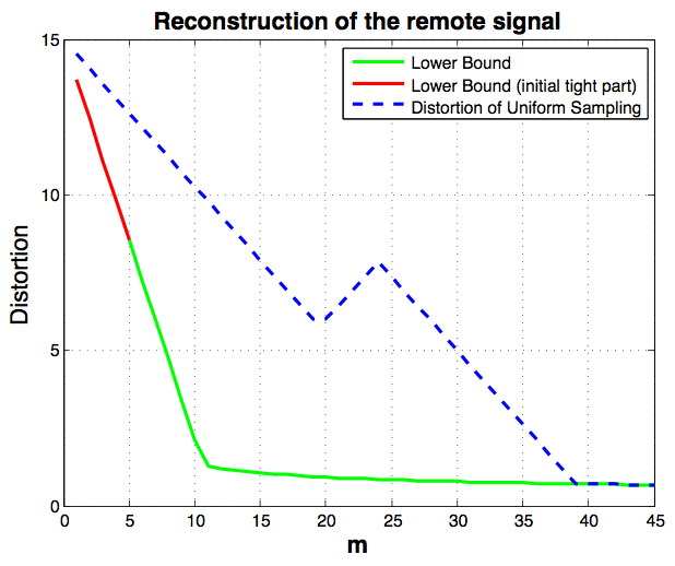
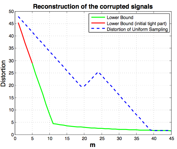
Figure 1: The the lower bound versus the distortion obtained by the uniform sampling strategy. It is assumed that $m_{i}=m$ for all $i$. The parameters for this figure are $(k,N_{1},N,N_{2},\sigma_{i}^{2},\eta)=(3,5,15,19,1,0.1)$.

Discussion 1: We know the exact value of optimal distortion for $m_{i}>2N_{2}$. As argued in Section 1.C, this corresponds to the high sampling rate region and is practically relevant when we have high sampling noise. If the sampling noise models the quantization error of an A/D converter, this result allows us to answer the question of whether it is better to collect some accurate samples from the signals, or collect many more less accurate samples from them (a problem related to selecting an appropriate $\Sigma\Delta$ modulator).

Discussion 2: Assume that the sampling noise variances of the corrupted signals satisfy $\sigma_{1}^{2}\leq\sigma_{2}^{2}\leq\cdots\leq\sigma_{k}^{2}$. Let us assume that we have a fixed total budget of $m$ samples that we can distribute among the $k$ signals, i.e., $\sum_{i=1}^{k}m_{i}=m$. Then if $m\leq N$, the lower bound will be tight. Regardless of whether we want to construct the original signal or the collection of corrupted signals, one can verify that the total distortion (subject to $\sum_{i=1}^{k}m_{i}=m$) is minimized when $m_{1}=m$ and $m_{i}=0$ for $i>1$, i.e., all of the samples are taken from the first signal, $S_{1}(t)$, which has the minimum sampling noise variance.
However, the problems of reconstructing the remote signal and the set of corrupted signals are not equivalent. To see this assume that we keep the constraint $\sum_{i=1}^{k}m_{i}=m$ for some $m>2N_{2}k$, and further assume that $m_{i}>2N_{2}$. For the reconstruction of the remote signal, it can be verified that the total distortion (subject to $\sum_{i=1}^{k}m_{i}=m,~{}~{}m_{i}>2N_{2}$) is minimized when $m_{i}$ for $i\geq 2$ reaches its minimum of $2N_{2}+1$, which means that we take as many samples as possible from the signal with minimum sampling noise variance $S_{1}(t)$. On the other hand, if we wish to minimize the total distortion of the entire corrupted signals, the optimum value for $m_{i}$ can vary depending on the value of the parameters; it is not necessarily true that it is better to sample from the less noisy signal. The intuitive reason for this is as follows: if sampling noise of a signal is very high, we need to take lots of samples from it to be able to have a reconstruction with low distortion. However, if the sampling noise of a signal is very low, we are able to have a good reconstruction with few samples; taking more samples yields a negligible improvement in distortion. Therefore, if we aim to reconstruct all the signals (i.e., to minimize the sum of the distortions of the signals), the most economic way could be taking less samples from the less noisy signal. For instance, let us consider the case of two signals, $k=2$, and take the corruption noise variance to be $\eta=0.5$. Assume that samples from the first signal are taken with variance $\sigma_{1}=1$, which is less than $\sigma_{2}=10$, the noise variance of samples from the second signal. Then for total sample budget $m=100$, the optimum $(m_{1},m_{2})$ subject to $m_{i}>2N_{2}$ is given in the following for different values of $N_{2}$. For $N_{2}=20$, the optimal choice is $(m_{1},m_{2})=(41,59)$; observe that it is better to take $59$ samples from the signal with more sampling noise. For $N_{2}=10$, the optimal choice is $(m_{1},m_{2})=(32,68)$. Here $m_{i}>2N_{2}=20$ and the optimal choice is not one of the boundary pairs $(m_{1},m_{2})=(21,79)$ or $(79,21)$.

3 Problem Formulation

In this section, we state the matrix representation of our problem. Let X be a column vector, consisting of the Fourier coefficients of $S(t)$

$$\textbf{X}=[{A_{N_{1}},A_{N_{1}+1},\cdots,A_{N_{2}},B_{N_{1}},\cdots,B_{N_{2}}}]^{\mathsf{T}},$$ (14)

where ^T is used for the transpose operation. Similarly, $\textbf{X}_{i}$ is a column vector, consisting of the coefficients of $S_{i}(t)$

$$\textbf{X}_{i} =[{A_{iN_{1}},A_{i(N_{1}+1)},\cdots,A_{iN_{2}},B_{iN_{1}},\cdots,B_{iN_{2}}}]^{\mathsf{T}}$$ (15)

$$=\textbf{X}+[{V_{iN_{1}},\cdots,V_{iN_{2}},W_{iN_{1}},\cdots,W_{iN_{2}}}]^{\mathsf{T}}$$ (16)

$$=\textbf{X}+\mathbf{\Delta}_{i},$$ (17)

where $\mathbf{\Delta}_{i}=[{V_{iN_{1}},\cdots,V_{iN_{2}},W_{iN_{1}},\cdots,W_{iN_{2}}}]^{\mathsf{T}}$. We assume that X consists of mutually independent Gaussian random variables $\mathcal{N}(0,1)$, i.e., the signal $S(t)$ is white. Therefore, $C_{\textbf{X}}=I_{2N\times 2N}$. Moreover, the random variables $V_{ij}$ and $W_{ij}$ are assumed to be independent with the probability distribution $\mathcal{N}(0,\eta)$ for some $\eta>0$.

Notation	Description	Helpful properties
$\mathbf{X}$	Column vector of size $2N$ of Fourier coefficients of $S(t)$	$C_{\mathbf{X}}=I_{2N\times 2N}$
$\mathbf{X}_{i}$	Column vector of size $2N$ of Fourier coefficients of $S_{i}(t)$	$C_{\textbf{X}_{i}}=(1+\eta)I$
	for $i=1,2,\cdots,k$	$C_{\textbf{X}_{i}\textbf{X}_{j}}=I$ for $i\neq j$
X	Vectors $\mathbf{X}_{i}$ Stacked on the bottom of each other; length $2Nk$	$C_{\textsf{{X}}}=\Lambda\otimes I_{2N\times 2N}$
$\Lambda$	Symmetric $k\times k$ matrix given in (18)
$\Gamma$	$\Gamma=\Lambda^{-1}$; Explicit formula given in (89)
$\mathbf{\Delta}_{i}$	The $i$th corruption vector: $\mathbf{\Delta}_{i}=\mathbf{X}_{i}-\mathbf{X}$	$C_{\mathbf{\Delta}_{i}}=\eta I_{2N\times 2N}$
$\boldsymbol{\mathsf{\Delta}}$	Column vectors $\mathbf{\Delta}_{i}$ Stacked on the bottom of each other	$C_{\textbf{C}}=\eta I_{2Nk\times 2Nk}$
$\mathbf{{S}}_{i}$	Column vector of size $m_{i}$; Samples of $S_{i}(t)$ at $t_{ij}$, $j=1,...,m_{i}$	$\mathbf{{S}}_{i}=Q_{i}\textbf{X}_{i}$
$Q_{i}$	$m_{i}\times 2N$ Matrix specified by harmonics at $t_{ij}$, given in (19)
$\mathsf{Q}_{\mathsf{a}}$	Matrices $Q_{i}$ stacked on the bottom of each other; size: $(\sum m_{i})\times 2N$
$\mathsf{Q}_{\mathsf{b}}$	Direct sum of matrices $Q_{i}$; size: $(\sum m_{i})\times 2Nk$
$\mathbf{Y}_{i}$	Noisy samples of the $i$th signal $S_{i}(t)$; length $m_{i}$	$\mathbf{Y}_{i}=\mathbf{S}_{i}+\mathbf{Z}_{i}$
Y	Vectors $\mathbf{Y}_{i}$ Stacked on the bottom of each other; length $m=\sum m_{i}$
$\mathbf{Z}_{i}$	Sampling noise vector of the $i$th signal $S_{i}(t)$; length $m_{i}$	$C_{\textbf{Z}_{i}}=\sigma_{i}^{2}I_{m_{i}\times m_{i}}$
Z	Vectors $\mathbf{Z}_{i}$ Stacked on the bottom of each other; length $m=\sum m_{i}$	$C_{\textsf{{Z}}}=\bigoplus_{i=1}^{k}\sigma_{i}^{2}I_{m_{i}\times m_{i}}$
$\boldsymbol{\mathsf{\tilde{Z}}}$	$\boldsymbol{\mathsf{\tilde{Z}}}$ is defined as $\mathsf{Q}_{\mathsf{b}}\mathsf{\boldsymbol{\mathsf{\Delta}}}+\textsf{{Z}}$. It appears in $\textsf{{Y}}=\mathsf{Q}_{\mathsf{a}}\mathbf{X}+\boldsymbol{\mathsf{\tilde{Z}}}.$	$C_{\boldsymbol{\mathsf{\tilde{Z}}}}=\eta\mathsf{Q}_{\mathsf{b}}\mathsf{Q}_{\mathsf{b}}^{\mathsf{T}}+C_{\textsf{{Z}}}$

Table 2: Definition of auxiliary parameters.

Vectors $\textbf{X}_{i}$ and $\textbf{X}_{j}$ are correlated, because they are both corrupted versions of X. Their cross covariance can be computed as $C_{\textbf{X}_{i}\textbf{X}_{i}}=(1+\eta)I$ and $C_{\textbf{X}_{i}\textbf{X}_{j}}=I$ for $i\neq j\in\{1,2,\cdots,k\}$. One can verify that for any $j$, the covariance matrix for the $k$ random variables $A_{ij}$ for $i=1,2,\cdots,k$ is equal to

$$\Lambda=\begin{pmatrix}{1+\eta}&{1}&{1}&\cdots&{1}\\ {1}&{1+\eta}&{1}&\cdots&{1}\\ \vdots&\vdots&\vdots&\vdots&\vdots\\ {1}&{1}&{1}&\cdots&{1+\eta}\end{pmatrix}_{k\times k}.$$ (18)

Suppose that the $i$th signal, $S_{i}(t)$, is sampled at time instances $t_{ij}$ for $i=1,2,\cdots,k$ and $j=1,2\cdots,m_{i}$. Hence,

$${S}_{i}(t_{ij})=\sum_{\ell=N_{1}}^{N_{2}}[{A}_{i\ell}\cos(\ell\omega t_{ij})+{B}_{i\ell}\sin(\ell\omega t_{ij})].$$

To represent the problem in a matrix form, we define $\mathbf{S}_{i}$ to be the vector of samples as

$$\mathbf{{S}}_{i}=[{S_{i}}(t_{i1}),{S_{i}}(t_{i2}),\cdots,{S_{i}}(t_{im_{i}})]^{\mathsf{T}}.$$

Therefore, we have $\mathbf{{S}}_{i}=Q_{i}\textbf{X}_{i}$, where $\textbf{X}_{i}$ is defined in (17) and $Q_{i}$ is an $m_{i}\times 2(N_{2}-N_{1}+1)=m_{i}\times 2N$ matrix of the form

$$Q_{i}=\begin{pmatrix}\cos(N_{1}\omega t_{i1})&\cos((N_{1}+1)\omega{t_{i1}})&\cdots&\cos(N_{2}\omega t_{i1})&\sin(N_{1}\omega t_{i1})&\sin((N_{1}+1)\omega t_{i1})&\cdots&\sin(N_{2}\omega t_{i1})\\ \cos(N_{1}\omega t_{i2})&\cos((N_{1}+1)\omega t_{i2})&\cdots&\cos(N_{2}\omega t_{i2})&\sin(N_{1}\omega t_{i2})&\sin((N_{1}+1)\omega t_{i2})&\cdots&\sin(N_{2}\omega t_{i2})\\ &&&\vdots&\vdots&&&\\ \cos(N_{1}\omega t_{im_{i}})&\cos((N_{1}+1)\omega t_{im_{i}})&\cdots&\cos(N_{2}\omega t_{im_{i}})&\sin(N_{1}\omega t_{im_{i}})&\sin((N_{1}+1)\omega t_{im_{i}})&\cdots&\sin(N_{2}\omega t_{im_{i}})\end{pmatrix}.$$ (19)

Moreover, the observation vector for the $i$th signal is of the following form

$$\mathbf{Y}_{i}=\mathbf{S}_{i}+\mathbf{Z}_{i}=Q_{i}\mathbf{X}_{i}+\mathbf{Z}_{i}=Q_{i}\mathbf{X}+Q_{i}\mathbf{\Delta}_{i}+\mathbf{Z}_{i},$$

in which $\mathbf{Z}_{i}$ is the $i$th noise vector with covariance of $C_{\textbf{Z}_{i}}=\sigma_{i}^{2}I_{m_{i}\times m_{i}}$.

Now, we define the vector of coefficients of all the $k$ signals, X, the vector of all the samples, S, the vector of all the observations, Y,… , as follows:

X $$=[\mathbf{X}_{1}^{\mathsf{T}},\mathbf{X}_{2}^{\mathsf{T}},\cdots,\mathbf{X}_{k}^{\mathsf{T}}]^{\mathsf{T}},$$ (20)

S $$=[\mathbf{S}_{1}^{\mathsf{T}},\mathbf{S}_{2}^{\mathsf{T}},\cdots,\mathbf{S}_{k}^{\mathsf{T}}]^{\mathsf{T}},$$ (21)

Y $$=[\mathbf{Y}_{1}^{\mathsf{T}},\mathbf{Y}_{2}^{\mathsf{T}},\cdots,\mathbf{Y}_{k}^{\mathsf{T}}]^{\mathsf{T}},$$ (22)

Z $$=[\mathbf{Z}_{1}^{\mathsf{T}},\mathbf{Z}_{2}^{\mathsf{T}},\cdots,\mathbf{Z}_{k}^{\mathsf{T}}]^{\mathsf{T}},$$ (23)

$$\boldsymbol{\mathsf{\Delta}} =[\mathbf{\Delta}_{1}^{\mathsf{T}},\mathbf{\Delta}_{2}^{\mathsf{T}},\cdots,\mathbf{\Delta}_{k}^{\mathsf{T}}]^{\mathsf{T}},$$ (24)

$$\mathsf{Q}_{\mathsf{a}} =[{Q}_{1}^{\mathsf{T}},{Q}_{2}^{\mathsf{T}},\cdots,{Q}_{k}^{\mathsf{T}}]^{\mathsf{T}}.$$ (25)

Furthermore, let

$$\mathsf{Q}_{\mathsf{b}}=\bigoplus_{i=1}^{k}Q_{i}$$ (26)

be the direct sum of the individual matrices $Q_{i}$. Then, we can write

$$\textsf{{Y}}=\textbf{{S}}+\textsf{{Z}}=\mathsf{Q}_{\mathsf{b}}\textsf{{X}}+\textsf{{Z}}=\mathsf{Q}_{\mathsf{a}}\mathbf{X}+\mathsf{Q}_{\mathsf{b}}\boldsymbol{\mathsf{\Delta}}+\textsf{{Z}}.$$ (27)

One can verify that the covariance matrix of the noise is

$$C_{\textsf{{Z}}}=\bigoplus_{i=1}^{k}C_{\textbf{Z}_{i}}=\bigoplus_{i=1}^{k}\sigma_{i}^{2}I_{m_{i}\times m_{i}}.$$ (28)

Moreover, $C_{\mathbf{X}}=I_{2N\times 2N}$ and $C_{\textsf{{X}}}=\Lambda\otimes I_{2N\times 2N}$, where $\Lambda$ was given in (18), and $N=N_{2}-N_{1}+1$.

3.1 Reconstruction of the remote signal $S(t)$ and its corrupted version $S_{i}(t)$

Here, we first state a lemma, which is frequently used in the formulation and proofs of our problem. The Lemma provides the two alternative forms of the LMMSE estimator and the mean squared error. Next we use this lemma to formulate the reconstruction of the remote signal $S(t)$ and its corrupted versions $S_{i}(t)$ in the subsequent subsections.

Lemma 1.

[20] Suppose that $\textbf{Y}=A\textbf{X}+\textbf{Z}$ in which Y is an observation vector, $A$ is a known matrix, X is a vector to be estimated and Z is an additive noise vector. In the case X and Z are mutually independent Gaussian vectors, LMMSE is optimal and the estimator and the mean square error, respectively, are given by

$$\hat{\mathbf{x}}_{\mathrm{MMSE}}(\mathbf{y}) =\mathbb{E}\left\{\mathbf{X}|\mathbf{y}\right\}=W\mathbf{y},$$

$$\mathbb{E}\|\mathbf{X}-\hat{\mathbf{X}}\|^{2} =\mathbb{E}_{\mathbf{Y}}\left\{\mathsf{Var}[\mathbf{X}|\mathbf{Y}]\right\}=\mathtt{Tr}(C_{e}),$$ (29)

where the reconstruction matrix, $W$, and the error covariance matrice, $C_{e}$, are of the following forms:

$$W =C_{\textbf{X}\textbf{Y}}C_{\textbf{Y}}^{-1}=C_{\textbf{X}}A^{\mathsf{T}}(AC_{\textbf{X}}A^{\mathsf{T}}+C_{\textbf{Z}})^{-1},$$

$$C_{e} =C_{\textbf{X}}-C_{\textbf{X}\textbf{Y}}C_{\textbf{Y}}^{-1}C_{\textbf{Y}\textbf{X}}=C_{\textbf{X}}-C_{\textbf{X}}A^{\mathsf{T}}(AC_{\textbf{X}}A^{\mathsf{T}}+C_{\textbf{Z}})^{-1}AC_{\textbf{X}}.$$ (30)

Or alternatively [21], using the matrix identity

$$C_{\textbf{X}}A^{\mathsf{T}}(AC_{\textbf{X}}A^{\mathsf{T}}+C_{\textbf{Z}})^{-1}=(A^{\mathsf{T}}C_{\textbf{Z}}^{-1}A+C_{\textbf{X}}^{-1})^{-1}A^{\mathsf{T}}C_{\textbf{Z}}^{-1},$$ (31)

the matrices $W$ and $C_{e}$ are given by

$$W =(A^{\mathsf{T}}C_{\textbf{Z}}^{-1}A+C_{\textbf{X}}^{-1})^{-1}A^{\mathsf{T}}C_{\textbf{Z}}^{-1},$$

$$C_{e} =(A^{\mathsf{T}}C_{\textbf{Z}}^{-1}A+C_{\textbf{X}}^{-1})^{-1}.$$ (32)

3.1.1 Reconstruction of $S(t)$

Here, the goal is to reconstruct $S(t)$ with minimum distortion using the observation vector Y. We use the MMSE criterion to minimize the average distortion subject to the samples. From the Parseval’s theorem, we have

$$\mathsf{D}_{\mathsf{a}}=\frac{1}{T}\int_{t=0}^{T}\mathbb{E}\{|\hat{S}(t)-S(t)|^{2}\}dt=\frac{1}{2}\mathbb{E}\|\mathbf{X}-\hat{\mathbf{X}}\|^{2},$$ (33)

where $\hat{S}(t)$ is the reconstructed signal and $\hat{\mathbf{X}}$ is the MMSE reconstruction of the coefficient vector $\mathbf{X}$ from the observation vector Y. Since the random variables are jointly Gaussian, the MMSE estimator is optimal. From the equation

$$\textsf{{Y}}=\mathsf{Q}_{\mathsf{a}}\mathbf{X}+\boldsymbol{\mathsf{\tilde{Z}}},$$

where $\boldsymbol{\mathsf{\tilde{Z}}}=\mathsf{Q}_{\mathsf{b}}\boldsymbol{\mathsf{\Delta}}+\textsf{{Z}}$, the error of the linear MMSE estiamtor is equal to

$$\mathbb{E}\|\mathbf{X}-\hat{\mathbf{X}}\|^{2} =\mathbb{E}_{\textsf{{Y}}}\left\{\mathsf{Var}[\mathbf{X}|\textsf{{Y}}]\right\}=\mathtt{Tr}(C^{\mathsf{a}}_{e}),$$ (34)

where $C^{\mathsf{a}}_{e}$ has the following two alternative forms

$$C^{\mathsf{a}}_{e} =C_{\mathbf{X}}-C_{\mathbf{X}}\mathsf{Q}_{\mathsf{a}}^{\mathsf{T}}(\mathsf{Q}_{\mathsf{a}}C_{\mathbf{X}}\mathsf{Q}_{\mathsf{a}}^{\mathsf{T}}+C_{\boldsymbol{\mathsf{\tilde{Z}}}})^{-1}\mathsf{Q}_{\mathsf{a}}C_{\mathbf{X}},$$ (35)

$$=(\mathsf{Q}_{\mathsf{a}}^{\mathsf{T}}C_{\boldsymbol{\mathsf{\tilde{Z}}}}^{-1}\mathsf{Q}_{\mathsf{a}}+C_{\mathbf{X}}^{-1})^{-1}.$$ (36)

In the above formula, the covariance matrix of $\boldsymbol{\mathsf{\tilde{Z}}}$ is

$$C_{\boldsymbol{\mathsf{\tilde{Z}}}}=\mathsf{Q}_{\mathsf{b}}C_{\boldsymbol{\mathsf{\Delta}}}\mathsf{Q}_{\mathsf{b}}^{\mathsf{T}}+C_{\textsf{{Z}}}=\eta\mathsf{Q}_{\mathsf{b}}\mathsf{Q}_{\mathsf{b}}^{\mathsf{T}}+C_{\textsf{{Z}}}.$$ (37)

3.1.2 Reconstruction of $S_{i}(t)$ for $i=1,2,\cdots,k$

Here, the goal is to reconstruct all the $k$ signals with minimum distortion using the observation vector Y. Again, from the Parseval’s theorem, we have

$$\mathsf{D}_{\mathsf{b}}=\frac{1}{T}\sum_{i=1}^{k}\int_{t=0}^{T}\mathbb{E}\{|\hat{S}_{i}(t)-S_{i}(t)|^{2}\}{d}t=\frac{1}{2}\mathbb{E}\|\textsf{{X}}-\hat{\textsf{{X}}}\|^{2},$$ (38)

in which $\hat{S}(t)$ and $\hat{\textsf{{X}}}$ are the reconstructed signal and the estimated coefficients, respectively. From the equation

$$\textsf{{Y}}=\mathsf{Q}_{\mathsf{b}}\textsf{{X}}+\textsf{{Z}},$$

the LMMSE error is equal to

$$\mathbb{E}\|\textsf{{X}}-\hat{\textsf{{X}}}^{2}\| =\mathbb{E}_{\textsf{{Y}}}\left\{\mathsf{Var}[\textsf{{X}}|\textsf{{Y}}]\right\}=\mathtt{Tr}(C^{\mathsf{b}}_{e}),$$ (39)

where $C^{\mathsf{b}}_{e}$ has the following two alternative forms

$$C^{\mathsf{b}}_{e} =C_{\textsf{{X}}}-C_{\textsf{{X}}}\mathsf{Q}_{\mathsf{b}}^{\mathsf{T}}(\mathsf{Q}_{\mathsf{b}}C_{\textsf{{X}}}\mathsf{Q}_{\mathsf{b}}^{\mathsf{T}}+C_{\textsf{{Z}}})^{-1}\mathsf{Q}_{\mathsf{b}}C_{\textsf{{X}}},$$ (40)

$$=(\mathsf{Q}_{\mathsf{b}}^{\mathsf{T}}C_{\textsf{{Z}}}^{-1}\mathsf{Q}_{\mathsf{b}}+C_{\textsf{{X}}}^{-1})^{-1}.$$ (41)

3.2 Some helpful facts

We provide a number of facts about the matrices that we have introduced before. These facts can be directly verified, and will be repeatedly used in the proofs. We have listed these facts here to improve the presentation of the proofs.

1. We have

   $$\mathsf{Q}_{\mathsf{b}}\mathsf{Q}_{\mathsf{b}}^{\mathsf{T}} =\bigoplus_{i=1}^{k}Q_{i}Q_{i}^{\mathsf{T}}=\begin{pmatrix}{{Q}_{1}{Q}_{1}^{\mathsf{T}}}&0&0&\cdots&0\\ 0&{{Q}_{2}{Q}_{2}^{\mathsf{T}}}&0&\cdots&0\\ \vdots&\vdots&\vdots&\vdots&\vdots\\ 0&0&0&\cdots&{{Q}_{k}{Q}_{k}^{\mathsf{T}}}\end{pmatrix}_{m\times m}$$ (42)

   and

   $$\mathsf{Q}_{\mathsf{a}}\mathsf{Q}_{\mathsf{a}}^{\mathsf{T}} =\begin{pmatrix}{{Q}_{1}{Q}_{1}^{\mathsf{T}}}&{{Q}_{1}{Q}_{2}^{\mathsf{T}}}&{{Q}_{1}{Q}_{3}^{\mathsf{T}}}&\cdots&{{Q}_{1}{Q}_{k}^{\mathsf{T}}}\\ {Q_{2}Q_{1}^{\mathsf{T}}}&{Q_{2}Q_{2}^{\mathsf{T}}}&{Q_{2}Q_{3}^{\mathsf{T}}}&\cdots&{Q_{2}Q_{k}^{\mathsf{T}}}\\ \vdots&\vdots&\vdots&\vdots&\vdots\\ {Q_{k}{Q}_{1}^{\mathsf{T}}}&{Q_{k}Q_{2}^{\mathsf{T}}}&{Q_{k}Q_{3}^{\mathsf{T}}}&\cdots&{Q_{k}Q_{k}^{\mathsf{T}}}\end{pmatrix}_{m\times m},$$ (43)

   where $m=\sum_{i=1}^{k}m_{i}$.

2. The rows of matrix $Q_{i}$ are vectors of norm $\sqrt{N}$. Therefore, the matrix $Q_{i}Q_{i}^{\mathsf{T}}$, for $i=1,2,\cdots,k$, is of size $m_{i}\times m_{i}$ and with diagonal entries equal to $N$ regardless of the value of $t_{ij}$. Therefore, $(\mathsf{Q}_{\mathsf{a}}\mathsf{Q}_{\mathsf{a}}^{\mathsf{T}})_{\mathsf{Diag}}=(\mathsf{Q}_{\mathsf{b}}\mathsf{Q}_{\mathsf{b}}^{\mathsf{T}})_{\mathsf{Diag}}=NI_{m\times m}$.

3. When, $t_{ij}\in\{0,T/N,\cdots,(N-1)T/N\}$ and are distinct, the rows of matrix ${Q}_{i}$ will be perpendicular to each other. Therefore, the matrix $Q_{i}Q_{i}^{\mathsf{T}}$ will be equal to $NI_{m_{i}\times m_{i}}$. Similarly, if $t_{ij}$ are distinct for all $i,j$, the rows of $Q_{i}$ and $Q_{j}$ for $i\neq j$ will be perpendicular to each other. Therefore, $Q_{i}Q_{j}^{\mathsf{T}}=0$ for $i\neq j$ in this case. Hence, using the definition of $\mathsf{Q}_{\mathsf{a}}$ and $\mathsf{Q}_{\mathsf{b}}$ given in (25) and (26), both $\mathsf{Q}_{\mathsf{a}}\mathsf{Q}_{\mathsf{a}}^{\mathsf{T}}$ and $\mathsf{Q}_{\mathsf{b}}\mathsf{Q}_{\mathsf{b}}^{\mathsf{T}}$ will become diagonal matrices $NI_{m\times m}$, where $m=\sum_{i=1}^{k}m_{i}$.

4. The diagonal elements of matrices $Q_{i}^{\mathsf{T}}Q_{i}$ for $i=1,2,\cdots,k$ give us the norm of the column vectors of $Q_{i}$. They can be calculated as follows:

   $$Q_{i}^{\mathsf{T}}Q_{i}(l,l)=\begin{cases}\sum_{j=1}^{{m_{i}}}\cos^{2}\left((N_{1}+l-1)\omega t_{ij}\right);&~{}~{}\text{for }1\leq l\leq N\\ \\ \sum_{j=1}^{m_{i}}\sin^{2}\left((N_{1}+l-N-1)\omega t_{ij}\right);&~{}~{}\text{for }N+1\leq l\leq 2N\end{cases}.$$ (44)

   When we use the uniform sampling strategy, i.e., $\{t_{ij}\}=\{0,T/m_{i},2T/m_{i},\cdots,(m_{i}-1)T/m_{i}\}$, the diagonal entries of $Q_{i}^{\mathsf{T}}Q_{i}$ will become equal to $m_{i}/2$. This is because, for instance,

   $$\sum_{j=1}^{{m_{i}}}\cos^{2}\left((N_{1}+l-1)\omega t_{ij}\right) =\sum_{j=0}^{{m_{i}-1}}\cos^{2}\left((N_{1}+l-1)\omega\frac{T}{m_{i}}j\right)$$

   $$=\sum_{j=0}^{{m_{i}-1}}\left(\frac{1}{2}+\frac{1}{2}\cos\Big{(}2(N_{1}+l-1)\frac{2\pi}{m_{i}}j\Big{)}\right)$$

   $$=\frac{m_{i}}{2},$$ (45)

   where (45) follows from the fact that $m_{i}>2N_{2}$. Moreover, the off-diagonal entries will be zero. For example, consider the entry

   $$Q_{i}^{\mathsf{T}}Q_{i}(2,3)=\sum_{j=1}^{{m_{i}}}\cos\left((N_{1}+1)\omega t_{ij}\right)\cos\left((N_{1}+2)\omega t_{ij}\right) =\sum_{j=0}^{{m_{i}-1}}\frac{1}{2}\left(\cos(\frac{\omega T}{m_{i}}j)+\cos\big{(}(2N_{1}+3)\frac{\omega T}{m_{i}}j\big{)}\right)$$

   $$=\sum_{j=0}^{{m_{i}-1}}\frac{1}{2}\left(\cos(\frac{2\pi}{m_{i}}j)+\cos\big{(}(2N_{1}+3)\frac{2\pi}{m_{i}}j\big{)}\right)$$

   $$=0.$$ (46)

   In fact, with uniform sampling, different columns of the matrix $Q_{i}$ will be perpendicular to each other and $Q_{i}^{\mathsf{T}}Q_{i}$ will become $(m_{i}/2)I_{2N\times 2N}$.

4 Proofs

In this section, we state the proofs of our results. In the body of the proofs, we have used some lemmas, which are provided in the appendix.

4.1 Proof of Equation (9)

We start by computing the average distortion using equations (33), (34) and (35) as follows

$$2\mathsf{D}_{\mathsf{a}}=\mathtt{Tr}(C^{\mathsf{a}}_{e}) =\mathtt{Tr}\left(C_{\mathbf{X}}-C_{\mathbf{X}}\mathsf{Q}_{\mathsf{a}}^{\mathsf{T}}(\mathsf{Q}_{\mathsf{a}}C_{\mathbf{X}}\mathsf{Q}_{\mathsf{a}}^{\mathsf{T}}+C_{\boldsymbol{\mathsf{\tilde{Z}}}})^{-1}\mathsf{Q}_{\mathsf{a}}C_{\mathbf{X}}\right)$$

$$=\mathtt{Tr}(C_{\mathbf{X}})-\mathtt{Tr}\left((\mathsf{Q}_{\mathsf{a}}C_{\mathbf{X}}\mathsf{Q}_{\mathsf{a}}^{\mathsf{T}}+C_{\boldsymbol{\mathsf{\tilde{Z}}}})^{-1}\mathsf{Q}_{\mathsf{a}}C_{\mathbf{X}}^{2}\mathsf{Q}_{\mathsf{a}}^{\mathsf{T}}\right)$$ (47)

$$=2N-\mathtt{Tr}\left((\mathsf{Q}_{\mathsf{a}}\mathsf{Q}_{\mathsf{a}}^{\mathsf{T}}+C_{\boldsymbol{\mathsf{\tilde{Z}}}})^{-1}\mathsf{Q}_{\mathsf{a}}\mathsf{Q}_{\mathsf{a}}^{\mathsf{T}}\right),$$ (48)

where (47) results from the cyclic property of the trace and (48) follows from the fact that $C_{\mathbf{X}}=I_{2N\times 2N}$.

We would like to show that for any arbitrary choice of sampling time instances, $t_{ij}$, the average distortion will be bounded from below as follows:

$$2\mathsf{D}_{\mathsf{a}} =2N-\mathtt{Tr}\left[(\mathsf{Q}_{\mathsf{a}}\mathsf{Q}_{\mathsf{a}}^{\mathsf{T}}+C_{\boldsymbol{\mathsf{\tilde{Z}}}})^{-1}\mathsf{Q}_{\mathsf{a}}\mathsf{Q}_{\mathsf{a}}^{\mathsf{T}}\right]$$

$$\geq 2N-N\sum_{i=1}^{k}\frac{m_{i}}{(1+\eta)N+\sigma_{i}^{2}}.$$ (49)

In other words, from (48), we wish to prove that

$$\mathtt{Tr}\left((\mathsf{Q}_{\mathsf{a}}\mathsf{Q}_{\mathsf{a}}^{\mathsf{T}}+C_{\boldsymbol{\mathsf{\tilde{Z}}}})^{-1}\mathsf{Q}_{\mathsf{a}}\mathsf{Q}_{\mathsf{a}}^{\mathsf{T}}\right)\leq\sum_{i=1}^{k}\frac{Nm_{i}}{(1+\eta)N+\sigma_{i}^{2}}.$$ (50)

Equivalently, if we use (37) to replace $C_{\boldsymbol{\mathsf{\tilde{Z}}}}$ with $(\eta\mathsf{Q}_{\mathsf{b}}\mathsf{Q}_{\mathsf{b}}^{\mathsf{T}}+C_{\textsf{{Z}}})$, we would like to show that

$$\mathtt{Tr}\left((\mathsf{Q}_{\mathsf{a}}\mathsf{Q}_{\mathsf{a}}^{\mathsf{T}}+\eta\mathsf{Q}_{\mathsf{b}}\mathsf{Q}_{\mathsf{b}}^{\mathsf{T}}+C_{\textsf{{Z}}})^{-1}\mathsf{Q}_{\mathsf{a}}\mathsf{Q}_{\mathsf{a}}^{\mathsf{T}}\right)\leq\sum_{i=1}^{k}\frac{Nm_{i}}{(1+\eta)N+\sigma_{i}^{2}}.$$ (51)

This can be derived using Theorem 3 (given in Appendix B) with matrices $F=\mathsf{Q}_{\mathsf{a}}\mathsf{Q}_{\mathsf{a}}^{\mathsf{T}}+\eta\mathsf{Q}_{\mathsf{b}}\mathsf{Q}_{\mathsf{b}}^{\mathsf{T}}$, $G=\mathsf{Q}_{\mathsf{a}}\mathsf{Q}_{\mathsf{a}}^{\mathsf{T}}$ and $C=C_{\textsf{{Z}}}$. From Fact (i) of Section 3.2, observe that the matrices $F$ and $G$ are of the forms

$$F=\begin{pmatrix}{(1+\eta)Q_{1}Q_{1}^{\mathsf{T}}}&{Q_{1}Q_{2}^{\mathsf{T}}}&{Q_{1}Q_{3}^{\mathsf{T}}}&\cdots&{Q_{1}Q_{k}^{\mathsf{T}}}\\ {Q_{2}Q_{1}^{\mathsf{T}}}&{(1+\eta)Q_{2}Q_{2}^{\mathsf{T}}}&{Q_{2}Q_{3}^{\mathsf{T}}}&\cdots&{Q_{2}Q_{k}^{\mathsf{T}}}\\ \vdots&\vdots&\vdots&\vdots&\vdots\\ {Q_{k}Q_{1}^{\mathsf{T}}}&{Q_{k}Q_{2}^{\mathsf{T}}}&{Q_{k}Q_{3}^{\mathsf{T}}}&\cdots&{(1+\eta)Q_{k}Q_{k}^{\mathsf{T}}}\end{pmatrix}_{m\times m}$$ (52)

and

$$G=\mathsf{Q}_{\mathsf{a}}\mathsf{Q}_{\mathsf{a}}^{\mathsf{T}}=\begin{pmatrix}{Q_{1}Q_{1}^{\mathsf{T}}}&{Q_{1}Q_{2}^{\mathsf{T}}}&{Q_{1}Q_{3}^{\mathsf{T}}}&\cdots&{Q_{1}Q_{k}^{\mathsf{T}}}\\ {Q_{2}Q_{1}^{\mathsf{T}}}&{Q_{2}Q_{2}^{\mathsf{T}}}&{Q_{2}Q_{3}^{\mathsf{T}}}&\cdots&{Q_{2}Q_{k}^{\mathsf{T}}}\\ \vdots&\vdots&\vdots&\vdots&\vdots\\ {Q_{k}Q_{1}^{\mathsf{T}}}&{Q_{k}Q_{2}^{\mathsf{T}}}&{Q_{k}Q_{3}^{\mathsf{T}}}&\cdots&{Q_{k}Q_{k}^{\mathsf{T}}}\end{pmatrix}_{m\times m}.$$ (53)

These matrices satisfy the required properties of Theorem 3, i.e., the matrices $F$ and $G$ are positive semi-definite and $G=F\circ L$, where the matrix $L$ has the form of (110) with parameters $a=1+\eta$ and $b=1$. Therefore, we have the following inequality

$$\mathtt{Tr}\left[\big{(}F+C\big{)}^{-1}G\right] \leq\mathtt{Tr}\left[\big{(}F_{\mathsf{Diag}}+C\big{)}^{-1}G_{\mathsf{Diag}}\right].$$ (54)

Hence, from Fact (ii) of Section 3.2 which states that $F_{\mathsf{Diag}}=(\mathsf{Q}_{\mathsf{a}}\mathsf{Q}_{\mathsf{a}}^{\mathsf{T}})_{\mathsf{Diag}}+\eta(\mathsf{Q}_{\mathsf{b}}\mathsf{Q}_{\mathsf{b}}^{\mathsf{T}})_{\mathsf{Diag}}=N(1+\eta)I_{m\times m}$ and $G_{\mathsf{Diag}}=(\mathsf{Q}_{\mathsf{a}}\mathsf{Q}_{\mathsf{a}}^{\mathsf{T}})_{\mathsf{Diag}}=NI_{m\times m}$, the desired inequality in (51) concludes.

Furthermore, when $\sum_{i=1}^{k}m_{i}\leq N$, we would like to show that this lower bound is tight if we take distinct time instances, $t_{ij}$, from the set $\{0,T/N,\cdots,(N-1)T/N\}$. Observe that this is possible since $\{0,T/N,\cdots,(N-1)T/N\}$ has $N$ elements. Fact (iii) from Section 3.2 states that both the matrices $\mathsf{Q}_{\mathsf{a}}\mathsf{Q}_{\mathsf{a}}^{\mathsf{T}}$ and $\mathsf{Q}_{\mathsf{b}}\mathsf{Q}_{\mathsf{b}}^{\mathsf{T}}$ will become diagonal matrices $NI_{m\times m}$, and thus $C_{\boldsymbol{\mathsf{\tilde{Z}}}}$ given in (37) will be

$$C_{\boldsymbol{\mathsf{\tilde{Z}}}} =\eta\mathsf{Q}_{\mathsf{b}}\mathsf{Q}_{\mathsf{b}}^{\mathsf{T}}+C_{\textsf{{Z}}}=\eta NI_{m\times m}+C_{\textsf{{Z}}}.$$

Hence, the minimum distortion will be

$$2\mathsf{D}_{\mathsf{a}\min} =2N-N\cdot\mathtt{Tr}\left[((1+\eta)NI+C_{\textsf{{Z}}})^{-1}\right],$$

$$=2N-\sum_{i=1}^{k}\frac{Nm_{i}}{(1+\eta)N+\sigma_{i}^{2}},$$ (55)

where (55) is derived using the definition of the diagonal matrix $C_{\textsf{{Z}}}$ given in (28). $\square$

4.2 Proof of equation (10):

To compute the minimum average distortion, from $\mathsf{D}_{\mathsf{a}}=1/2\mathtt{Tr}(C^{\mathsf{a}}_{e})$, we use the alternative form of LMMSE (given in (36)), in which $C^{\mathsf{a}}_{e}$ is of the form

$$C^{\mathsf{a}}_{e}=(\mathsf{Q}_{\mathsf{a}}^{\mathsf{T}}C_{\boldsymbol{\mathsf{\tilde{Z}}}}^{-1}\mathsf{Q}_{\mathsf{a}}+C_{\mathbf{X}}^{-1})^{-1}.$$ (56)

Hence, the average distortion will be

$$2\mathsf{D}_{\mathsf{a}}=\mathtt{Tr}(C^{\mathsf{a}}_{e})=\mathtt{Tr}\left[\left(\sum_{i=1}^{k}{Q_{i}^{\mathsf{T}}(\eta Q_{i}Q_{i}^{\mathsf{T}}+\sigma_{i}^{2}I)^{-1}Q_{i}}+I\right)^{-1}\right],$$ (57)

which results from the facts that $C_{\boldsymbol{\mathsf{\tilde{Z}}}}=\eta\mathsf{Q}_{\mathsf{b}}\mathsf{Q}_{\mathsf{b}}^{\mathsf{T}}+C_{\textsf{{Z}}}$ (Section 3.1.1) and $C_{\mathbf{X}}=I_{2N\times 2N}$.

Using the matrix identity given in (31) for matrix $A$ to be $\sqrt{\eta}Q_{i}$, we have

$$Q_{i}^{\mathsf{T}}\left(\eta Q_{i}Q_{i}^{\mathsf{T}}+C_{\textbf{Z}_{i}}\right)^{-1}Q_{i}=\left(\eta Q_{i}^{\mathsf{T}}C_{\textbf{Z}_{i}}^{-1}Q_{i}+I\right)^{-1}Q_{i}^{\mathsf{T}}C_{\textbf{Z}_{i}}^{-1}Q_{i}.$$

Therefore, the matrix in the left-hand side of (57) will be

$$\sum_{i=1}^{k}Q_{i}^{\mathsf{T}}\left(\eta Q_{i}Q_{i}^{\mathsf{T}}+C_{\textbf{Z}_{i}}\right)^{-1}Q_{i} =\sum_{i=1}^{k}\left(\eta Q_{i}^{\mathsf{T}}C_{\textbf{Z}_{i}}^{-1}Q_{i}+I\right)^{-1}Q_{i}^{\mathsf{T}}C_{\textbf{Z}_{i}}^{-1}Q_{i}$$

$$=\frac{1}{\eta}\sum_{i=1}^{k}\left(\eta Q_{i}^{\mathsf{T}}Q_{i}+\sigma_{i}^{2}I\right)^{-1}\left(\eta Q_{i}^{\mathsf{T}}Q_{i}+\sigma_{i}^{2}I-\sigma_{i}^{2}I\right)$$ (58)

$$=\frac{1}{\eta}\sum_{i=1}^{k}\left(I-\left(\eta\frac{Q_{i}^{\mathsf{T}}Q_{i}}{\sigma_{i}^{2}}+I\right)^{-1}\right)$$

$$=\frac{1}{\eta}\sum_{i=1}^{k}(I-B_{i})$$ (59)

$$=\frac{1}{\eta}(kI-\sum_{i=1}^{k}B_{i})$$

$$\leq\frac{1}{\eta}\left(kI-k^{2}\Big{(}\sum_{i=1}^{k}B_{i}^{-1}\Big{)}^{-1}\right),$$ (60)

where (58) results from the fact that $C_{\textbf{Z}_{i}}=\sigma^{2}_{i}I$, and in (59) matrix $B_{i}$ stands for $\left(\eta{Q_{i}^{\mathsf{T}}Q_{i}}/{\sigma_{i}^{2}}+I\right)^{-1}$. Moreover, (60) is derived using Lemma 4 for positive definite matrices $B_{i}$ with the equality if and only if $B_{1}=B_{2}=\cdots=B_{k}$. Notice that $0<B_{i}\leq I$.

For any two symmetric positive definite matrices $A$ and $B$, the relation $A\leq B$ implies that $B^{-1}\leq A^{-1}$. This is because the function $f(t)=-t^{-1}$ is operator monotone [27]. Hence, (60) implies that

$$\left(I+\sum_{i=1}^{k}{Q_{i}^{\mathsf{T}}(\eta Q_{i}Q_{i}^{\mathsf{T}}+\sigma_{i}^{2}I)^{-1}Q_{i}}\right)^{-1} \geq\left[I+\frac{1}{\eta}\left({k}I-k^{2}\Big{(}\sum_{i=1}^{k}B_{i}^{-1}\Big{)}^{-1}\right)\right]^{-1}.$$

Let $A=\sum_{i=1}^{k}B_{i}^{-1}=\sum_{i=1}^{k}\left(\eta{Q_{i}^{\mathsf{T}}Q_{i}}/{\sigma_{i}^{2}}+I\right)$. Then, the relation between the traces of the above matrices is

$$\mathtt{Tr}\left(I+\sum_{i=1}^{k}{Q_{i}^{\mathsf{T}}(\eta Q_{i}Q_{i}^{\mathsf{T}}+\sigma_{i}^{2}I)^{-1}Q_{i}}\right)^{-1} \geq\mathtt{Tr}\left[I+\frac{1}{\eta}\left({k}I-k^{2}A^{-1}\right)\right]^{-1}$$

$$\geq\mathtt{Tr}\left[I+\frac{1}{\eta}\left({k}I-k^{2}A_{\mathsf{Diag}}^{-1}\right)\right]^{-1},$$ (61)

where (61) results from Lemma 3 for the convex function $f(t)=(1+k/\eta-k^{2}t^{-1}/\eta)^{-1}$ when $t\geq k$ and the Hermitian matrix $A\geq kI$. To find $A_{\mathsf{Diag}}$, we need to calculate the diagonal entries of matrix $A$. They are

$$A(l,l)=\begin{cases}\sum_{i=1}^{{k}}\left(1+\sum_{j=1}^{{m_{i}}}\frac{\eta}{\sigma_{i}^{2}}\cos^{2}\big{(}(N_{1}+l-1)\omega t_{ij}\big{)}\right)\triangleq a_{\ell};&~{}~{}\text{for }1\leq l\leq N\\ \\ \sum_{i=1}^{{k}}\left(1+\sum_{j=1}^{m_{i}}\frac{\eta}{\sigma_{i}^{2}}\sin^{2}\big{(}(N_{1}+l-N-1)\omega t_{ij}\big{)}\right)\triangleq b_{\ell};&~{}~{}\text{for }N+1\leq l\leq 2N\end{cases},$$ (62)

since the diagonal elements of matrices $Q_{i}^{\mathsf{T}}Q_{i}$ for $i=1,2,\cdots,k$ are of the following forms (Fact (iv) from Section 3.2)

$$Q_{i}^{\mathsf{T}}Q_{i}(l,l)=\begin{cases}\sum_{j=1}^{{m_{i}}}\cos^{2}\left((N_{1}+l-1)\omega t_{ij}\right);&~{}~{}\text{for }1\leq l\leq N\\ \\ \sum_{j=1}^{m_{i}}\sin^{2}\left((N_{1}+l-N-1)\omega t_{ij}\right);&~{}~{}\text{for }N+1\leq l\leq 2N\end{cases}.$$ (63)

Substituting the diagonal entries of the matrix $A$ in (61), we obtain

$$\mathtt{Tr}\left(I+\sum_{i=1}^{k}{Q_{i}^{\mathsf{T}}(\eta Q_{i}Q_{i}^{\mathsf{T}}+\sigma_{i}^{2}I)^{-1}Q_{i}}\right)^{-1} \geq\mathtt{Tr}\left[I+\frac{1}{\eta}\left({k}I-k^{2}A_{\mathsf{Diag}}^{-1}\right)\right]^{-1}$$

$$=\sum_{\ell=1}^{N}\frac{1}{(1+\frac{k}{\eta})-\frac{k^{2}}{\eta}a_{\ell}^{-1}}+\frac{1}{(1+\frac{k}{\eta})-\frac{k^{2}}{\eta}b_{\ell}^{-1}}$$

$$\geq\sum_{\ell=1}^{N}\frac{2}{(1+\frac{k}{\eta})-\frac{k^{2}}{\eta}(k+\eta\sum_{i=1}^{k}\frac{m_{i}}{2\sigma_{i}^{2}})^{-1}}$$ (64)

$$=\frac{2N}{(1+\frac{k}{\eta})-\frac{k^{2}}{\eta}(k+\eta\sum_{i=1}^{k}\frac{m_{i}}{2\sigma_{i}^{2}})^{-1}},$$ (65)

where (64) results from convexity of the function $f(t)=(1-at^{-1})^{-1}$ for $t\geq a$.

Now suppose that each $m_{i}>2N_{2}$ for $i=1,2,\cdots,k$. If we uniformly sample the signals, i.e., sample $S_{i}(t)$ at time instances $\{0,T/m_{i},2T/m_{i},\cdots,(m_{i}-1)T/m_{i}\}$, from Fact (iv) of Section 3.2 we conclude that the equality in the above equations holds, and thus the this lower bound is achieved.

$\square$

4.3 Proof of Equation (12):

To compute the average distortion, here we use equations (38), (39) and (41). Hence,

$$2\mathsf{D}_{\mathsf{b}} =\mathtt{Tr}\left(C_{\textsf{{X}}}-C_{\textsf{{X}}}\mathsf{Q}_{\mathsf{b}}^{\mathsf{T}}(\mathsf{Q}_{\mathsf{b}}C_{\textsf{{X}}}\mathsf{Q}_{\mathsf{b}}^{\mathsf{T}}+C_{\textsf{{Z}}})^{-1}\mathsf{Q}_{\mathsf{b}}C_{\textsf{{X}}}\right)$$

$$=\mathtt{Tr}(C_{\textsf{{X}}})-\mathtt{Tr}\left((\mathsf{Q}_{\mathsf{b}}C_{\textsf{{X}}}\mathsf{Q}_{\mathsf{b}}^{\mathsf{T}}+C_{\textsf{{Z}}})^{-1}\mathsf{Q}_{\mathsf{b}}C_{\textsf{{X}}}^{2}\mathsf{Q}_{\mathsf{b}}^{\mathsf{T}}\right)$$ (66)

$$=k(2N)(1+\eta)-\mathtt{Tr}\left((\mathsf{Q}_{\mathsf{b}}C_{\textsf{{X}}}\mathsf{Q}_{\mathsf{b}}^{\mathsf{T}}+C_{\textsf{{Z}}})^{-1}\mathsf{Q}_{\mathsf{b}}C_{\textsf{{X}}}^{2}\mathsf{Q}_{\mathsf{b}}^{\mathsf{T}}\right),$$ (67)

where (66) and (67) are achieved, respectively, by the trace cyclic property and the fact that $C_{\textsf{{X}}}=\Lambda\otimes I_{2N\times 2N}$ (The matrix $\Lambda$ has been defined in (18)).

Here we are interested in reconstructing the signals $S_{i}(t)$. Following the similar steps from Subsection 4.1, we use Theorem 3 with the choice of $F=\mathsf{Q}_{\mathsf{b}}C_{\textsf{{X}}}\mathsf{Q}_{\mathsf{b}}^{\mathsf{T}}$, $G=\mathsf{Q}_{\mathsf{b}}C_{\textsf{{X}}}^{2}\mathsf{Q}_{\mathsf{b}}^{\mathsf{T}}$ and $C=C_{\textsf{{Z}}}$. To demonstrate that these matrices have the required properties of Theorem 3, one can verify (by explicit evaulation) that $F$ has the same expression as in (52), i.e., $F=\mathsf{Q}_{\mathsf{b}}C_{\textsf{{X}}}\mathsf{Q}_{\mathsf{b}}^{\mathsf{T}}=\mathsf{Q}_{\mathsf{b}}(\Lambda\otimes I_{2N\times 2N})\mathsf{Q}_{\mathsf{b}}^{\mathsf{T}}$ is also equal to $\mathsf{Q}_{\mathsf{a}}\mathsf{Q}_{\mathsf{a}}^{\mathsf{T}}+\eta\mathsf{Q}_{\mathsf{b}}\mathsf{Q}_{\mathsf{b}}^{\mathsf{T}}.$ Furthermore to compute $G$, observe that $C_{X}^{2}=\Lambda^{2}\otimes I_{2N\times 2N}$ in which ${\Lambda}^{2}$ is a matrix of the following form

$$\Lambda^{2}(i,j)=\begin{cases}(1+\eta)^{2}+(k-1)\triangleq\alpha~{}~{};~{}~{}i=j,\\ \\ 2(1+\eta)+(k-2)\triangleq\beta~{}~{};~{}~{}i\neq j,\end{cases}$$ (68)

for $i,j=1,2,\cdots,k$. Then, one can verify that

$$G=\begin{pmatrix}{\alpha Q_{1}Q_{1}^{\mathsf{T}}}&{\beta Q_{1}Q_{2}^{\mathsf{T}}}&{\beta Q_{1}Q_{3}^{\mathsf{T}}}&\cdots&{\beta Q_{1}Q_{k}^{\mathsf{T}}}\\ {\beta Q_{2}Q_{1}^{\mathsf{T}}}&{\alpha Q_{2}Q_{2}^{\mathsf{T}}}&{\beta Q_{2}Q_{3}^{\mathsf{T}}}&\cdots&{\beta Q_{2}Q_{k}^{\mathsf{T}}}\\ \vdots&\vdots&\vdots&\vdots&\vdots\\ {\beta Q_{k}Q_{1}^{\mathsf{T}}}&{\beta Q_{k}Q_{2}^{\mathsf{T}}}&{\beta Q_{k}Q_{3}^{\mathsf{T}}}&\cdots&{\alpha Q_{k}Q_{k}^{\mathsf{T}}}\end{pmatrix}_{m\times m}.$$ (69)

Therefore, applying Theorem 3 for the matrices $F$, $G$ and $C=C_{\textsf{{Z}}}$, we have

$$\mathtt{Tr}\left((\mathsf{Q}_{\mathsf{b}}C_{\textsf{{X}}}\mathsf{Q}_{\mathsf{b}}^{\mathsf{T}}+C_{\textsf{{Z}}})^{-1}\mathsf{Q}_{\mathsf{b}}C_{\textsf{{X}}}^{2}\mathsf{Q}_{\mathsf{b}}^{\mathsf{T}}\right) =\mathtt{Tr}[(F+C_{\textsf{{Z}}})^{-1}G]$$

$$\leq\mathtt{Tr}[(F_{\mathsf{Diag}}+C_{\textsf{{Z}}})^{-1}G_{\mathsf{Diag}}]$$

$$=\mathtt{Tr}\left[\big{(}(1+\eta)NI+C_{\textsf{{Z}}}\big{)}^{-1}\alpha NI\right]$$ (70)

$$=\sum_{i=1}^{k}\frac{\alpha Nm_{i}}{(1+\eta)N+\sigma_{i}^{2}},$$ (71)

where (70) results from the fact that the diagonal entries of the matrices $F$ and $G$ are $(1+\eta)N$ and $\alpha N$, respectively (Fact (ii) from Section 3.2 and (69)). Consequently, the average distortion, for any arbitrary choice of sampling times, can be bounded as

$$2\mathsf{D}_{\mathsf{b}} =2Nk(1+\eta)-\mathtt{Tr}\left((\mathsf{Q}_{\mathsf{b}}C_{\textsf{{X}}}\mathsf{Q}_{\mathsf{b}}^{\mathsf{T}}+C_{\textsf{{Z}}})^{-1}\mathsf{Q}_{\mathsf{b}}C_{\textsf{{X}}}^{2}\mathsf{Q}_{\mathsf{b}}^{\mathsf{T}}\right)$$

$$\geq 2Nk(1+\eta)-\sum_{i=1}^{k}\frac{\alpha Nm_{i}}{(1+\eta)N+\sigma_{i}^{2}},$$

in which $\alpha$ is the one defined in (68).

Furthermore, we would like to show that the equality holds when $\sum_{i=1}^{k}m_{i}\leq N$ and we take distinct time instances, $t_{ij}$, from the set $\{0,T/N,\cdots,(N-1)T/N\}$. To show that we compute the average distortion when $t_{ij}$ are distinct and belong to $\{0,T/N,\cdots,(N-1)T/N\}$ for all $i,j$. Using Fact (iii) from Section 3.2, the two matrices $F$ and $G$ will become diagonal matrices of the forms:

$$F=\mathsf{Q}_{\mathsf{b}}C_{\textsf{{X}}}\mathsf{Q}_{\mathsf{b}}^{\mathsf{T}}=(1+\eta)NI_{m\times m},~{}~{}~{}G=\mathsf{Q}_{\mathsf{b}}C_{\textsf{{X}}}^{2}\mathsf{Q}_{\mathsf{b}}^{\mathsf{T}}=\alpha NI_{m\times m}$$ (72)

Hence, the average distortion will be

$$2\mathsf{D}_{\mathsf{b}\min} =2Nk(1+\eta)-\mathtt{Tr}\left(((1+\eta)NI_{m\times m}+C_{\textsf{{Z}}})^{-1}\alpha NI_{m\times m}\right)$$ (73)

$$=2Nk(1+\eta)-\sum_{i=1}^{k}\frac{\alpha Nm_{i}}{(1+\eta)N+\sigma_{i}^{2}}$$ (74)

where (74) is derived using the diagonal matrix $C_{\textsf{{Z}}}$ of (28). $\square$

4.4 Proof of Equation (13):

Here, we divide the proof into two parts. In the first part, we show that

$$\mathsf{D}_{\mathsf{b}\min}\geq N\cdot\mathtt{Tr}\left(\mathsf{Diag}([\frac{m_{1}}{2\sigma_{1}^{2}},\frac{m_{2}}{2\sigma_{2}^{2}},\cdots,\frac{m_{k}}{2\sigma_{k}^{2}}])+\Gamma\right)^{-1},$$

and then we show that when $m_{i}>2N_{2}$ (for each $i\in{1,2,\cdots,k}$), the optimal sampling strategy is uniform sampling and the minimum distortion is equal to

$$\mathsf{D}_{\mathsf{b}\min}=N\cdot\mathtt{Tr}\left(\mathsf{Diag}([\frac{m_{1}}{2\sigma_{1}^{2}},\frac{m_{2}}{2\sigma_{2}^{2}},\cdots,\frac{m_{k}}{2\sigma_{k}^{2}}])+\Gamma\right)^{-1}.$$

In the second part, we simplify the above equation to obtain the expression given in the statement of the theorem.

Part (i): To compute the minimum average distortion, we use $\mathsf{D}_{\mathsf{b}}=1/2\mathtt{Tr}(C^{\mathsf{b}}_{e})$ and the alternative form of LMMSE, where $C^{\mathsf{b}}_{e}$ is of the form

$$C^{\mathsf{b}}_{e}=\left(\mathsf{Q}_{\mathsf{b}}^{\mathsf{T}}C_{\textsf{{Z}}}^{-1}\mathsf{Q}_{\mathsf{b}}+C_{\textsf{{X}}}^{-1}\right)^{-1}.$$ (75)

In the above formula,

$$C_{\textsf{{Z}}}^{-1}=\bigoplus_{i=1}^{k}\frac{1}{\sigma^{2}_{i}}I_{2N\times 2N},\quad C_{\textsf{{X}}}^{-1}=\Gamma_{k\times k}\otimes I_{2N\times 2N},$$ (76)

where the matrix $\Gamma$ is the inverse of the matrix $\Lambda$, given in (18). Therefore, the average distortion will be

$$2\mathsf{D}_{\mathsf{b}}=\mathtt{Tr}(C^{\mathsf{b}}_{e})=\mathtt{Tr}\left[\left(\bigoplus_{i=1}^{k}\frac{Q_{i}^{\mathsf{T}}Q_{i}}{\sigma_{i}^{2}}\right)+\Gamma\otimes I\right]^{-1}.$$ (77)

First notice that due to Lemma 5, matrices $\Gamma\otimes I$ and $I\otimes\Gamma$ are permutation similar, i.e., there exists a unique permutation matrix $P(k,2N)$ of size $2Nk\times 2Nk$ such that

$$\Gamma\otimes I=P(k,2N)^{T}(I\otimes\Gamma)P(k,2N),$$

and moreover, $P(k,2N)$ has the property

$$P(k,2N)=P(k,2N)^{T}=P(k,2N)^{-1}.$$

Using the permutation matrix $P(k,2N)$ and the cyclic property of the trace, we have

$$2\mathsf{D}_{\mathsf{b}}=\mathtt{Tr}(C^{\mathsf{b}}_{e}) =\mathtt{Tr}\left(P(k,2N)^{T}C^{\mathsf{b}}_{e}P(k,2N)\right)$$

$$=\mathtt{Tr}\left[P(k,2N)^{T}\left(\bigoplus_{i=1}^{k}\frac{Q_{i}^{\mathsf{T}}Q_{i}}{\sigma_{i}^{2}}\right)P(k,2N)+P(k,2N)^{T}\left(\Gamma\otimes I\right)P(k,2N)\right]^{-1}$$

$$=\mathtt{Tr}\left(H+I\otimes\Gamma\right)^{-1},$$ (78)

where matrix $H$ denotes the permuted matrix $P(k,2N)^{T}(\bigoplus_{i=1}^{k}{Q_{i}^{\mathsf{T}}Q_{i}}/{\sigma_{i}^{2}})P(k,2N)$. Notice that the matrix

$$\bigoplus_{i=1}^{k}{Q_{i}^{\mathsf{T}}Q_{i}}=\sum_{i=1}^{k}G_{i}\otimes Q_{i}^{\mathsf{T}}Q_{i},$$

where $G_{i}$ is a $k\times k$ matrix defined as follows: $G_{i}(i^{\prime},j^{\prime})=0$ if $(i^{\prime},j^{\prime})\neq(i,i)$, and $G_{i}(i^{\prime},j^{\prime})=1$ if $(i^{\prime},j^{\prime})=(i,i)$. Therefore, the matrix $H$ can be written as

$$H =P(k,2N)^{T}(\bigoplus_{i=1}^{k}{Q_{i}^{\mathsf{T}}Q_{i}}/{\sigma_{i}^{2}})P(k,2N)$$

$$=\sum_{i=1}^{k}Q_{i}^{\mathsf{T}}Q_{i}\otimes G_{i}.$$ (79)

If we partition $H$ into $k\times k$ submatrices $H_{ij}$ as follows

$$H=\begin{pmatrix}{H_{11}}&{H_{12}}&\cdots&H_{1(2N)}\\ {H_{21}}&{H_{22}}&\cdots&{H_{2(2N)}}\\ \vdots&\vdots&\vdots&\vdots\\ {H_{(2N)1}}&{H_{(2N)2}}&\cdots&{H_{(2N)(2N)}}\end{pmatrix},$$ (80)

all the $H_{ij}$ submatrices will be diagonal matrices because they are weighted sums of diagonal matrices $G_{i}$. More precisely, the submatrices $H_{ll}$ for $l\leq N$ can be computed as follows, using Fact (iv) from Section 3.2 that gives us the diagonal entries of $Q_{i}^{\mathsf{T}}Q_{i}$ (the entries of matrix $H_{ll}$ for $1\leq l\leq N$ and $N\leq l\leq 2N$ are the $l$th and the $(l+N)$th diagonal entries of matrices $Q_{i}^{\mathsf{T}}Q_{i}/\sigma_{i}^{2}$, given in (63)), respectively):

$$H_{ll}=\begin{pmatrix}{\frac{1}{\sigma_{1}^{2}}\sum_{j=1}^{{m_{1}}}{\cos^{2}\scriptstyle\left((N_{1}+l-1)\omega t_{1j}\right)}}&{0}&{0}&\cdots&{0}\\ {0}&{\frac{1}{\sigma_{2}^{2}}\sum_{j=1}^{m_{2}}\cos^{2}\scriptstyle\left((N_{1}+l-1)\omega t_{2j}\right)}&{0}&\cdots&{0}\\ \vdots&\vdots&\vdots&\vdots&\vdots\\ {0}&{0}&{0}&\cdots&{\frac{1}{\sigma_{k}^{2}}\sum_{j=1}^{{m_{k}}}\cos^{2}\scriptstyle\left((N_{1}+l-1)\omega t_{kj}\right)}\end{pmatrix}_{k\times k}$$

and for $l=N+1,N+2,\cdots,2N$,

$$H_{ll}=\begin{pmatrix}{\frac{1}{\sigma_{1}^{2}}\sum_{j=1}^{{m_{1}}}\sin^{2}\scriptstyle\left((N_{1}+l-N-1)\omega t_{1j}\right)}&{0}&{0}&\cdots&{0}\\ {0}&{\frac{1}{\sigma_{2}^{2}}\sum_{j=1}^{{m_{2}}}\sin^{2}\scriptstyle\left((N_{1}+l-N-1)\omega t_{2j}\right)}&{0}&\cdots&{0}\\ \vdots&\vdots&\vdots&\vdots&\vdots\\ {0}&{0}&{0}&\cdots&{\frac{1}{\sigma_{k}^{2}}\sum_{j=1}^{{m_{k}}}\sin^{2}\scriptstyle\left((N_{1}+l-N-1)\omega t_{kj}\right)}\end{pmatrix}_{k\times k}$$

Applying Lemma 3 for the Hermitian matrix $A$ and the convex function $f(x)=x^{-1}$ for $x>0$, we attain a lower bound on the average distortion as:

$$2\mathsf{D}_{\mathsf{b}}=\mathtt{Tr}(C^{\mathsf{b}}_{e}) =\mathtt{Tr}\left(H+I\otimes\Gamma\right)^{-1},$$

$$\geq\mathtt{Tr}\left(H_{\mathsf{B}\mathsf{Diag}}+I\otimes\Gamma\right)^{-1},$$ (81)

in which the matrix $H_{\mathsf{B}\mathsf{Diag}}$ is the block diagonal form of matrix $H$, where all the submatrices other than the $2N$ block diagonal submatrices, ${H}_{ll}$, are zero. Consequently, the matrix $(H_{\mathsf{B}\mathsf{Diag}}+I\otimes\Gamma)$ is of the form

$$(H_{\mathsf{B}\mathsf{Diag}}+I\otimes\Gamma)=\begin{pmatrix}{H_{11}+\Gamma}&{0}&{\cdots}&{0}\\ {0}&{H_{22}+\Gamma}&{\cdots}&{0}\\ \vdots&\vdots&\vdots&\vdots\\ {0}&{0}&\cdots&{H_{(2N)(2N)}+\Gamma}\end{pmatrix}_{2Nk\times 2Nk}.$$ (82)

Therefore,

$$\mathtt{Tr}\left(H_{\mathsf{B}\mathsf{Diag}}+I\otimes\Gamma\right)^{-1}=\sum_{l=1}^{2N}\mathtt{Tr}\left(H_{ll}+\Gamma\right)^{-1}.$$

Using Lemma 6 (given in Appendix B), for any $1\leq l\leq N$, we obtain

$$\frac{1}{2}(\mathtt{Tr}\left(H_{ll}+\Gamma\right)^{-1}+\mathtt{Tr}\left(H_{(l+N)(l+N)}+\Gamma\right)^{-1}) \geq\mathtt{Tr}\left(\frac{1}{2}(H_{ll}+H_{(l+N)(l+N)})+\Gamma\right)^{-1}$$ (83)

$$=\mathtt{Tr}\left(\mathsf{Diag}([\frac{m_{1}}{2\sigma_{1}^{2}},\frac{m_{2}}{2\sigma_{2}^{2}},\cdots,\frac{m_{k}}{2\sigma_{k}^{2}}])+\Gamma\right)^{-1}.$$ (84)

Consequently,

$$\ \mathtt{Tr}\left(H_{\mathsf{B}\mathsf{Diag}}+I\otimes\Gamma\right)^{-1}=\sum_{l=1}^{2N}\mathtt{Tr}\left(H_{ll}+\Gamma\right)^{-1}\geq 2N\cdot\mathtt{Tr}\left(\mathsf{Diag}([\frac{m_{1}}{2\sigma_{1}^{2}},\frac{m_{2}}{2\sigma_{2}^{2}},\cdots,\frac{m_{k}}{2\sigma_{k}^{2}}])+\Gamma\right)^{-1}.$$ (85)

Therefore, from (81) for any choice of sampling time instances $t_{ij}$, we obtain

$$\mathsf{D}_{\mathsf{b}}\geq N\cdot\mathtt{Tr}\left(\mathsf{Diag}([\frac{m_{1}}{2\sigma_{1}^{2}},\frac{m_{2}}{2\sigma_{2}^{2}},\cdots,\frac{m_{k}}{2\sigma_{k}^{2}}])+\Gamma\right)^{-1}.$$ (86)

Moreover, suppose that each $m_{i}>2N_{2}$ for $i=1,2,\cdots,k$. If we employ uniform strategy, the matrices $Q_{i}^{\mathsf{T}}Q_{i}$ ($i=1,2,\cdots,k$) become diagonal matrices with diagonal entries equal to $m_{i}/2$ (Fact (iv) from Section 3.2). Then, the matrix in the right hand side of (77) will be

$$\left[\left(\bigoplus_{i=1}^{k}\frac{m_{i}}{2\sigma_{i}^{2}}I_{2N\times 2N}\right)+\Gamma\otimes I\right]^{-1} =\left(\mathsf{Diag}([\frac{m_{1}}{2\sigma_{1}^{2}},\frac{m_{2}}{2\sigma_{2}^{2}},\cdots,\frac{m_{k}}{2\sigma_{k}^{2}}])\otimes I+\Gamma\otimes I\right)^{-1}$$ (87)

$$=\left(\mathsf{Diag}([\frac{m_{1}}{2\sigma_{1}^{2}},\frac{m_{2}}{2\sigma_{2}^{2}},\cdots,\frac{m_{k}}{2\sigma_{k}^{2}}])+\Gamma\right)^{-1}\otimes I_{2N\times 2N}.$$ (88)

Therefore, from (77) and the fact that $\mathtt{Tr}(A\otimes B)=\mathtt{Tr}(A)\mathtt{Tr}(B)$, we get

$$\mathsf{D}_{\mathsf{b}\min}\leq N\cdot\mathtt{Tr}\left(\mathsf{Diag}([\frac{m_{1}}{2\sigma_{1}^{2}},\frac{m_{2}}{2\sigma_{2}^{2}},\cdots,\frac{m_{k}}{2\sigma_{k}^{2}}])+\Gamma\right)^{-1}.$$

Therefore, from (LABEL:) and the above inequality, we conclude that

$$\mathsf{D}_{\mathsf{b}\min}=N\cdot\mathtt{Tr}\left(\mathsf{Diag}([\frac{m_{1}}{2\sigma_{1}^{2}},\frac{m_{2}}{2\sigma_{2}^{2}},\cdots,\frac{m_{k}}{2\sigma_{k}^{2}}])+\Gamma\right)^{-1}.$$

Part (ii): So far we have shown that when $m_{i}>2N_{2}$ for $i=1,2,\cdots,k$, the minimal distortion is

$$\mathsf{D}_{\mathsf{b}\min}=N\cdot\mathtt{Tr}\left(\mathsf{Diag}([\frac{m_{1}}{2\sigma_{1}^{2}},\frac{m_{2}}{2\sigma_{2}^{2}},\cdots,\frac{m_{k}}{2\sigma_{k}^{2}}])+\Gamma\right)^{-1}.$$

Here, we wish to simplify the above equation to obtain Observe that $\Gamma=\Lambda^{-1}$ can be computed from (18) as follows:

$$\Gamma=\begin{pmatrix}{\mathsf{a}}&{\mathsf{b}}&{\mathsf{b}}&\cdots&{\mathsf{b}}\\ {\mathsf{b}}&{\mathsf{a}}&{\mathsf{b}}&\cdots&{\mathsf{b}}\\ \vdots&\vdots&\vdots&\vdots&\vdots\\ {\mathsf{b}}&{\mathsf{b}}&{\mathsf{b}}&\cdots&{\mathsf{a}}\end{pmatrix}_{k\times k},$$ (89)

in which

$$\mathsf{a}=\frac{\eta+k-1}{\eta(\eta+k)}~{}~{}\text{ and }~{}~{}\mathsf{b}=\frac{-1}{\eta(\eta+k)}.$$ (90)

For simplicity define:

$$A:=\mathsf{Diag}([\frac{m_{1}}{2\sigma_{1}^{2}},\frac{m_{2}}{2\sigma_{2}^{2}},...,\frac{m_{k}}{2\sigma_{k}^{2}}])+\Gamma$$ (91)

Therefore, we need to find $\mathtt{Tr}(A^{-1})$ which is equal to $\sum_{i=1}^{k}(A^{-1})_{i,i}$. To calculate the diagonal entries of $A^{-1}$, we use the Cramer’s rule as follows:

$$(A^{-1})_{i,i}=\frac{\det(A_{i})}{\det(A)}$$ (92)

where $A_{i}$ is the remaining matrix after removing the $i$th row and column of $A$. According to Lemma 7 (given in Appendix B), we deduce:

$$(A^{-1})_{i,i}=\frac{\prod\limits_{\begin{subarray}{c}j=1\\ j\neq i\end{subarray}}^{k}\phi_{j}+\mathsf{b}\sum\limits_{\begin{subarray}{c}j=1\\ j\neq i\end{subarray}}^{k}\prod\limits_{\begin{subarray}{c}l=1\\ l\neq i,j\end{subarray}}^{k}\phi_{l}}{\prod\limits_{j=1}^{k}\phi_{j}+\mathsf{b}\sum\limits_{j=1}^{k}\prod\limits_{\begin{subarray}{c}l=1\\ l\neq j\end{subarray}}^{k}\phi_{l}}$$ (93)

in which $\phi_{i}=\frac{m_{i}}{2\sigma_{i}^{2}}+\mathsf{a}-\mathsf{b}=\frac{m_{i}}{2\sigma_{i}^{2}}+\frac{1}{\eta}$. Hence,

$$\mathtt{Tr}(A^{-1}) =\sum_{i=1}^{k}(A^{-1})_{i,i}$$ (94)

$$=\frac{\sum\limits_{i=1}^{k}\frac{1}{\phi_{i}}+\mathsf{b}\sum\limits_{\begin{subarray}{c}i,j=1\\ j\neq i\end{subarray}}^{k}\frac{1}{\phi_{i}\phi_{j}}}{1+\mathsf{b}(\sum\limits_{i=1}^{k}\frac{1}{\phi_{i}})},$$ (95)

in which (95) is derived by replacing (93) in (94) and dividing both numerator and denominator by $\prod\limits_{i=1}^{k}\phi_{i}$. Observe that by our definition $\Phi_{-1}:=\sum\limits_{i=1}^{k}\frac{1}{\phi_{i}}$, we get

$$\mathtt{Tr}(A^{-1})=\frac{\Phi_{-1}+\mathsf{b}(\Phi_{-1}^{2}-\sum\limits_{i=1}^{k}\frac{1}{\phi_{i}^{2}})}{1+\mathsf{b}\Phi_{-1}}=\Phi_{-1}-\frac{\mathsf{b}}{1+\mathsf{b}\Phi_{-1}}\Phi_{-2}.$$ (96)

We get the desired result by replacing $\mathsf{b}=-1/(\eta(\eta+k))$. $\square$

Appendix A Lemmas

In this section, we state some lemmas that have been used in the proof section.

A.1 Majorization inequalities

A vector $\textbf{x}\in\mathbb{R}^{n}$ is majorized by $\textbf{y}\in\mathbb{R}^{n}$ if after sorting the two vectors in decreasing order, the following inequalities hold:

$$\sum_{i=1}^{k}x_{i}\leq\sum_{i=1}^{k}y_{i}\quad(1\leq k\leq n),\quad\sum_{i=1}^{n}x_{i}=\sum_{i=1}^{n}y_{i}.$$ (97)

A fundamental result in majorization theory states that for any Hermitian matrix $A$ of size $n\times n$, the diagonal entries of $A$ are majorized by its eigenvalues [22]. The extension of the above result to the block Hermitian matrices is also true (e.g. see [23, Sec. 1]):

Lemma 2 (Block majorization inequality).

If a Hermitian matrix $A$ is partitioned into block matrices

$$A=\begin{pmatrix}M_{11}&M_{12}&\dots&M_{1k}\\ M_{21}&M_{22}&\dots&M_{2k}\\ \vdots&&\vdots\\ M_{k1}&M_{k2}&\dots&M_{kk}\end{pmatrix}$$ (98)

for matrices $M_{ij},{i,j=1,2,\dots,k}$, then the eigenvalues of $\bigoplus_{i=1}^{k}M_{ii}$ are majorized by the eigenvalues of $A$.

If a vector x is majorized by y, then for any convex functions $f:\mathbb{R}\mapsto\mathbb{R}$, we have $\sum_{i}f(x_{i})\leq\sum_{i}f(y_{i})$ [22]. This implies that

Lemma 3.

Let $\Omega$ be a closed interval in $\mathbb{R}$. For any Hermitian matrix $A$ with eigenvalues in $\Omega$, and any convex function $f$ on $\Omega$,

$$\mathtt{Tr}(f(A))\geq\mathtt{Tr}(f(A_{\mathsf{Diag}})).$$ (99)

More generally by Lemma 2 , for a Hermitian matrix $A$ partitioned into block matrices $M_{ij},{i,j=1,2,\dots,k}$, as in (98),

$$\mathtt{Tr}(f(A))\geq\mathtt{Tr}\left(f\Big{(}\bigoplus_{i=1}^{k}M_{ii}\Big{)}\right).$$ (100)

A.2 Other useful definitions and inequalities

Lemma 4.

[24] Let $w_{1},w_{2},\cdots,w_{k}$ be non-negative weights adding up to one, and let $B_{1},B_{2},\cdots,B_{k}$ be $n\times n$ positive definite matrices. Consider the weighted arithmetic and harmonic means of the matrices $B_{i}$

$$A \triangleq w_{1}B_{1}+w_{2}B_{2}+\cdots+w_{k}B_{k},$$ (101)

$$H \triangleq(w_{1}B_{1}^{-1}+w_{2}B_{2}^{-1}+\cdots+w_{k}B_{k}^{-1})^{-1}.$$ (102)

Then, the following inequality holds,

$$H\leq A,$$

with equality if and only if $B_{1}=B_{2}=\cdots=B_{k}$.

Definition 1.

[25] A real-valued continuous function $f(t)$ on a real interval $I$ is called operator monotone if

$$A\leq B~{}~{}\Rightarrow~{}~{}f(A)\leq f(B),$$ (103)

for Hermitian matrices $A$ and $B$ with eigenvalues in $I$ . Furthermore, $f$ is called operator convex if

$$f(\lambda A+(1-\lambda)B)\leq\lambda f(A)+(1-\lambda)f(B),$$

for any $0\leq\lambda\leq 1$ and Hermitian matrices $A$ and $B$ with eigenvalues that are contained in $I$, and $f$ is said to be operator concave if $-f$ is operator convex.

Lemma 5.

[26, p.260] Let $m$ and $n$ be given positive integers and matrices $A$ and $B$ be any square matrices of sizes $m\times m$ and $n\times n$, respectively. Then, matrix $B\otimes A$ is permutation similar to matrix $A\otimes B$, i.e., there is a unique matrix $P$ such that

$$B\otimes A=P(m,n)^{T}(A\otimes B)P(m,n)$$ (104)

where $P(m,n)$ is the following $mn\times mn$ permutation matrix:

$$P(m,n)=\sum_{i=1}^{n}\sum_{j=1}^{m}E_{ij}\otimes E_{ij}^{T}$$ (105)

in which $E_{ij}$ is an $m\times n$ matrix such that only the $(i,j)$th entry is unity and the other entries are zero. Furthermore, the useful following property holds

$$P(m,n)=P(n,m)^{T}=P(n,m)^{-1}.$$ (106)

Lemma 6.

Assume that $B_{1},B_{2}$ are positive definite matrices. Let $B=(B_{1}+B_{2})/2$, then

$$2\mathtt{Tr}(B^{-1})\leq\mathtt{Tr}(B_{1}^{-1})+\mathtt{Tr}(B_{2}^{-1}).$$

Proof.

The Löwner-Heinz theorem implies that the function $f(t)=t^{-1}$ for $t>0$ is operator convex [27]. From the fact that $B=(B_{1}+B_{2})/2$, we conclude the desired inequality.

Lemma 7.

Given real non-negative $a_{1},a_{2},...,a_{k}$ and positive $b$, let

$$M(a_{1},..,a_{k},b):=\begin{pmatrix}{a_{1}}&{-b}&{-b}&\cdots&{-b}\\ {-b}&{a_{2}}&{-b}&\cdots&{-b}\\ \vdots&\vdots&\vdots&\vdots&\vdots\\ {-b}&{-b}&{-b}&\cdots&{a_{k}}\end{pmatrix}_{k\times k}.$$ (107)

Then,

$$\det(M(a_{1},...,a_{k},b))=\prod_{i=1}^{k}(a_{i}+b)-b\sum_{i=1}^{k}\prod_{\begin{subarray}{c}j=1\\ j\neq i\end{subarray}}^{k}(a_{j}+b).$$ (108)

Proof.

The elementary row operations do not change the determinant. If we first subtract the first row from all the other rows, and then multiply the $i$th row of the matrix by ${b}/{(a_{i}+b)}$ for $i=2,3,..,k$, and add it to the first row, we end up with an upper triangular matrix with diagonal entries $\{a^{\prime},a_{2}+b,a_{3}+b,...,a_{k}+b\}$, where $a^{\prime}=a_{1}-\sum_{i=2}^{k}\frac{(a_{1}+b)b}{(a_{i}+b)}.$ Since the determinant of an upper triangular matrix is equal to product of the diagonal elements, we have

$$\begin{split}\det(M(a_{1},...,a_{k},b))&=a^{\prime}(a_{2}+b)...(a_{k}+b)\\ &=a_{1}(a_{2}+b)...(a_{k}+b)-b\sum_{i=2}^{k}\prod_{\begin{subarray}{c}j=1\\ j\neq i\end{subarray}}^{k}(a_{j}+b)\\ &=\prod_{i=1}^{k}(a_{i}+b)-b\sum_{i=1}^{k}\prod_{\begin{subarray}{c}j=1\\ j\neq i\end{subarray}}^{k}(a_{j}+b).\end{split}$$ (109)

Appendix B A new reverse majorization inequality

Theorem 3.

Take two positive semidefinite matrices $F$ and $G$ of sizes $m\times m$ satisfying $G=F\circ L$, where $\circ$ is the Hadamard product and $L$ is a matrix of the following form:

$$L=\begin{pmatrix}{a\mathbf{1}_{m_{1}\times m_{1}}}&{b\mathbf{1}_{m_{1}\times m_{2}}}&\cdots&{b\mathbf{1}_{m_{1}\times m_{k}}}\\ {b\mathbf{1}_{m_{2}\times m_{1}}}&{a\mathbf{1}_{m_{2}\times m_{2}}}&\cdots&{b\mathbf{1}_{m_{2}\times m_{k}}}\\ \vdots&\vdots&\vdots&\vdots\\ {b\mathbf{1}_{m_{k}\times m_{1}}}&{b\mathbf{1}_{m_{k}\times m_{2}}}&\cdots&{a\mathbf{1}_{m_{k}\times m_{k}}}\end{pmatrix},$$ (110)

where $\mathbf{1}$ is a matrix with all one coordinates and $a$ and $b$ are two positive real numbers, where $0\leq a\leq b$. Then, for any positive definite diagonal matrix $C$, we have

$$\mathtt{Tr}\left[\big{(}F+C\big{)}^{-1}G\right] \leq\mathtt{Tr}\left[\big{(}F_{\mathsf{Diag}}+C\big{)}^{-1}G_{\mathsf{Diag}}\right],$$ (111)

where $F_{\mathsf{Diag}}$ is a diagonal matrix formed by taking the diagonal entries of $F$, and the matrix $G_{\mathsf{Diag}}$ is defined similarly.

Proof.

If the statement of theorem holds for the matrix $F$, it will also hold for the matrix $kF$ for any positive constant $k$. Therefore, without loss of generality, we assume that $a=1$ and hence, $b\geq 1$. From the Hadamard product relation, this implies that $F$ and $G$ are equal on block matrices on the diagonal. Let $A$ denote this common part, i.e.,

$$A=\begin{pmatrix}{F_{1:m_{1}\times 1:m_{1}}}&0&0&\cdots&0\\ 0&{F_{(m_{1}+1:m_{1}+m_{2})\times(m_{1}+1:m_{1}+m_{2})}}&0&\cdots&0\\ \vdots&\vdots&\vdots&\vdots&\vdots\\ 0&0&0&\cdots&{F_{(m_{1}+\cdots+m_{k-1}+1)\times(m_{1}+\cdots+m_{k-1}+m_{k})}}\end{pmatrix}_{m\times m}.$$

One can find matrix $B$ such that $F=A+B$ and $G=A+bB$. Observe that wherever $A$ is non-zero, $B$ is zero and vice versa. Substituting $F$ and $G$ in the left hand side of (111), one attains

$$\mathtt{Tr}\left[\big{(}F+C\big{)}^{-1}G\right] =\mathtt{Tr}\left[\big{(}A+B+C\big{)}^{-1}\big{(}A+bB\big{)}\right]$$

$$=\mathtt{Tr}\left[(A+B+C)^{-1}(A+B)\right]+\mathtt{Tr}\left[(A+B+C)^{-1}(b-1)B)\right].$$ (112)

We will show that the first term in the above formula is less than or equal to the right hand side of (111) and the second term is non-positive.

Start with the first term of (112)

$$\mathtt{Tr}\left[(A+B+C)^{-1}(A+B)\right]=\mathtt{Tr}(I_{m\times m})-\mathtt{Tr}\left((A+B+C)^{-1}C\right),$$ (113)

where the second term in (113) can be bounded as follows:

$$\mathtt{Tr}\left((A+B+C)^{-1}C\right) =\mathtt{Tr}\left[\big{(}C^{\frac{-1}{2}}AC^{\frac{-1}{2}}+C^{\frac{-1}{2}}BC^{\frac{-1}{2}}+I\big{)}^{-1}\right]$$

$$\geq\mathtt{Tr}\left[\big{(}C^{\frac{-1}{2}}A_{\mathsf{Diag}}C^{\frac{-1}{2}}+I\big{)}^{-1}\right].$$ (114)

The last inequality comes from Lemma 3.
Hence, (113) will be bounded as

$$\mathtt{Tr}\left[(A+B+C)^{-1}(A+B)\right] \leq\mathtt{Tr}(I_{m\times m})-\mathtt{Tr}\left[\big{(}C^{\frac{-1}{2}}A_{\mathsf{Diag}}C^{\frac{-1}{2}}+I\big{)}^{-1}\right],$$ (115)

$$=\mathtt{Tr}[(A_{\mathsf{Diag}}+C)^{-1}(A_{\mathsf{Diag}}+C)]-\mathtt{Tr}[C^{\frac{1}{2}}(A_{\mathsf{Diag}}+C)^{-1}C^{\frac{1}{2}}]$$ (116)

$$=\mathtt{Tr}[(A_{\mathsf{Diag}}+C)^{-1}A_{\mathsf{Diag}}]$$ (117)

$$=\mathtt{Tr}[(F_{\mathsf{Diag}}+C)^{-1}G_{\mathsf{Diag}}],$$ (118)

in which (117) comes from the trace interchange property and (118) is derived since $A$ is defined to be the common part of the two matrices $F$ and $G$.

To complete the proof, it remains to show that the right hand side of (112) is non-positive, i.e.,

$$(b-1)\cdot\mathtt{Tr}\left[(A+B+C)^{-1}B\right]\leq 0.$$ (119)

Since we have assumed that $b\geq 1$, we need to show that the trace function is non-positive. For the positive definite matrix $(A+C)$, we have

$$\mathtt{Tr}\left((A+B+C)^{-1}B\right) =\mathtt{Tr}(I)-\mathtt{Tr}\left((A+C+B)^{-1}(A+C)\right)$$

$$=\mathtt{Tr}(I)-\mathtt{Tr}\left((A+C)^{\frac{1}{2}}(A+C+B)^{-1}(A+C)^{\frac{1}{2}}\right)$$ (120)

$$=\mathtt{Tr}(I)-\mathtt{Tr}\left((I+(A+C)^{\frac{-1}{2}}B(A+C)^{\frac{-1}{2}})^{-1}\right)$$

$$\leq\mathtt{Tr}(I)-\mathtt{Tr}(I)$$ (121)

$$=0.$$

in which the inequality (120) follows from the trace interchange property and (121) is derived using Lemma 3 for the Hermitian matrix $(I+(A+C)^{\frac{1}{2}}B(A+C)^{\frac{1}{2}})^{-1}$. Note that the matrix $(A+C)^{\frac{1}{2}}B(A+C)^{\frac{1}{2}}$ is a block off-diagonal matrix, since matrices $A$ and $B$ has been defined to be, respectively, block diagonal and off-diagonal matrices such that wherever $A_{ij}$ is zero, $B_{ij}$ is non-zero and vice versa. This completes the proof of Theorem 3.

References

- [1] T. Berger, Rate-Distortion Theory, Wiley Online Library, 1971.
- [2] H. Witsenhausen, “Indirect rate distortion problems,” IEEE Trans. Inf. Theory, vol. 26, no. 5, pp. 518–521, Sep. 1980.
- [3] J. Wolf and J. Ziv, “Transmission of noisy information to a noisy receiver with minimum distortion,” IEEE Trans. Inf. Theory, vol.16, no. 4, pp. 406–411, Apr. 1970.
- [4] R. Dobrushin and B. Tsybakov, “Information transmission with additional noise,” IRE Trans. Inf. Theory, vol. 8, no. 5, pp. 293–304, Jun. 1962.
- [5] T. Berger, Z. Zhang and and H. Viswanathan, “The CEO problem [multiterminal source coding],” IEEE Trans. Inf. Theory, vol. 42, no .3, pp. 887-902, 1996.
- [6] H. Viswanathan, and T. Berger, “The quadratic Gaussian CEO problem,” IEEE Trans. Inf. Theory, vol. 43, no. 5, pp. 1549-1559, 1997.
- [7] E. Mohammadi and F. Marvasti, “Sampling and Distortion Tradeoffs for Bandlimited Periodic Signals,” Sampling Theory and Applications (SampTA), 2015 International Conference on, pp. 468 - 472, arXiv 1405.3980.
- [8] D. Baron, M. B. Wakin, M. F. Duarte, S. Sarvotham, and R. G. Baraniuk, “Distributed Compressed Sensing,” Elect. Comput. Eng. Dep., Rice University, Houston, TX, Tech. Rep. ECE-0612, Dec. 2006.
- [9] A. Hormati, O. Roy, Y.M. Lu and M. Vetterli, “Distributed sampling of signals linked by sparse filtering: Theory and applications,” IEEE Trans. Signal Process., 58(3), pp.1095-1109, 2010.
- [10] A. Ahmed and J. Romberg, “Compressive Sampling of Ensembles of Correlated Signals,” arXiv:1501.06654, 2015.
- [11] D. Ganesan, D. Estrin and J. Heidemann,“DIMENSIONS: Why do we need a new data handling architecture for sensor networks?,” ACM SIGCOMM Computer Communication Review, 33(1), pp.143-148, 2003.
- [12] S. Bandyopadhyay, Q. Tian and E.J. Coyle, “Spatio-temporal sampling rates and energy efficiency in wireless sensor networks,” IEEE/ACM Transactions on Networking (TON) 13, no. 6, pp. 1339-1352, 2005.
- [13] D. Zordan, G. Quer, M. Zorzi and M. Rossi, “Modeling and generation of space-time correlated signals for sensor network fields,” IEEE Global Telecommunications Conference (GLOBECOM 2011), (pp. 1-6).
- [14] R. Masiero, G. Quer, D. Munaretto, M. Rossi, J. Widmer, and M. Zorzi, “Data Acquisition through joint Compressive Sensing and Principal Component Analysis,” in IEEE Globecom 2009, Honolulu, Hawaii, US, Nov.-Dec. 2009.
- [15] W.Bajwa, J.Haupt, A.Sayeed, and R.Nowak,“Compressive wireless sensing,” in Proc. Int. Conf. Inf. Process. Sens. Netw., Apr. 2006, pp. 134–142.
- [16] W. Wang, M. Garofalakis, and K. Ramchandran, “Distributed sparse random projections for refinable approximation,” in Proc. Int. Conf. Inf. Process. Sens. Netw., Apr. 2007, pp. 331–339.
- [17] A. Kipnis, A. Goldsmith, Y. C. Eldar and T. Weissman, “Distortion Rate Function of sub-Nyquist Sampled Gaussian Sources,” IEEE Trans. Inf. Theory, vol. 62, no. 1, pp. 401-429, Jan. 2016.
- [18] S. Feizi, V. K. Goyal and M. Medard, “Time-stampless adaptive nonuniform sampling for stochastic signals”, IEEE Trans. Signal Process., vol. 60, no. 10, pp. 5440-5450, Oct. 2012.
- [19] V. P. Boda and P. Narayan, “Sampling rate distortion,” in Proc. IEEE Int. Symp. on Inf. Theory (ISIT), 2014, pp. 3057 - 3061.
- [20] S. M. Kay, Fundamentals of statistical signal processing: Estimation theory, Prentice-Hall, Inc., Upper Saddle River, NJ, USA, 1993.
- [21] D. G. Luenberger, Optimization by vector space methods, John Wiley & Sons, 1990.
- [22] R. Bhatia, Matrix analysis, Springer Science & Business Media, 1997.
- [23] M. Lin and and H. Wolkowicz, “An eigenvalue majorization inequality for positive semidefinite block matrices,” Linear and Multilinear Algebra, no. 60.11-12, pp. 1365-1368, 2012.
- [24] M. Sagae and K. Tanabe, “Upper and lower bounds for the arithmetic-geometric-harmonic means of positive definite matrices,” Linear and Multilinear Algebra, pp. 279-282, 1994.
- [25] X. Zhan, Matrix inequalities, Springer Science & Business Media, 2002.
- [26] R. A. Horn and C. R. Johnson, Topics in matrix analysis, Vol. 2, Camb. Univ. Press, England, 1991.
- [27] E. Carlen, “Trace inequalities and quantum entropy: an introductory course,” Entropy and the quantum 529, pp. 73-140, 2010.