Physical and Geometrical Parameters of CVBS xi@: COU1511 (HIP12552)

Abstract

Model atmospheres of the close visual binary star COU1511 (HIP12552) are constructed using grids of Kuruz’s blanketed models to build the individual synthetic SEDs for both components. These synthetic SED’s are combined together for the entire system and compared with the observational one following Al-Wardat’s complex method for analyzing close visual binary stars. The entire observational spectral energy distribution (SED) of the system is used as a reference for comparison between synthetic SED and the observed one. The parameters of both components are derived as: $T_{\rm eff}^{a}=6180\pm 50$ K, $T_{\rm eff}^{b}=5865\pm 70$ K, log $g_{a}=4.35\pm 0.12$, log $g_{b}=4.45\pm 0.14$, $R_{a}=1.262\pm 0.08R_{\odot}$, $R_{b}=1.006\pm 0.07R_{\odot}$, $L_{a}=2.09\pm 0.10L_{\odot}$, $L_{b}=1.08\pm 0.12L_{\odot}$, with spectral types F8 and G1 for both components (a,b) respectively, and age of $3.0\pm 0.9$ Gy. A modified orbit of the system is built and the masses of the two components are calculated as $M_{a}=1.17\pm 0.11M_{\odot}$, $M_{b}=1.06\pm 0.10M_{\odot}$.

1 INTRODUCTION

Recent surveys of the sky showed that more than 50% of the galactic stellar systems are binaries, which raises their importance in understanding the formation and evolution of the galaxy. This role in determining precisely different stellar parameters gives the study of binary stars a special importance. The case is a bit complicated in the case of close visual binary stars (CVBS), which are not resolved as binaries by inspecting limited images, but can be resolved in space based observations, or by using modern techniques of ground-based observations, like speckle interferometry and adaptive optics.

In addition to that, Docobo et al. (2001) pointed out that the study of orbital motion of visual and interferometric pairs remains an important astronomical discipline. The visual binaries are the main key source of information about stellar masses and distances, and they define practically our understanding of stellar physical properties especially for the lower part of the main sequence stars .

For now, hundreds of CVBS with periods on the order of 10 years or less are routinely observed by different groups of high resolution techniques around the world. This has helped in determining the orbital parameters and magnitude differences for some of these CVBS. However, this is not sufficient to determine the individual physical parameters of the components of the system.

Al-Wardat’s method for analyzing CVBS (Al-Wardat 2012) offers a complementary solution for this problem by implementing differential photometry, spectrophotometry, atmospheric modeling, and orbital solution in accurate determination of different physical and geometrical parameters of this category of stars. The method was successfully applied to several solar type and subgaint binary systems such as Hip70973, Hip72479 (Al-Wardat 2012), Hip689 (Al-Wardat et al. 2014), and Hip11253 (Al-Wardat & Widyan 2009).

As a consequence of the previous work, this paper (the XI in its series) presents the analysis of the nearby solar type CVBS COU1511 (Hip12552), with a modification to its parallax.

Table 1 shows the basic data of the system taken from SIMBAD and NACA/IPAC catalogues, and Table 2 shows data from Hipparcos and Tycho catalogues (ESA 1997), while Table 3 shows the magnitude difference of the system along with filters used to observe them.

Table 1: Basic data of the system

	Hip12552	Reference
$\alpha_{2000}$	$02^{h}41^{m}28\hbox{$.\!\!^{s}$}88$	SIMBAD†
$\delta_{2000}$	$+40\hbox{${}^{\circ}$}52^{\prime}50.^{\prime\prime}84$	-
Tyc.	2849-1282-1	-
HD	16656	-
Sp. Typ.	G0	-
$E(B-V)$	$0.076\pm 0.002$	NASA/IPAC∗
$A_{v}$	$0\hbox{$.\!\!^{m}$}24$	NASA/IPAC

^† http://simbad.u-strasbg.fr/simbad/

^∗ http://irsa.ipac.caltech.edu,

Table 2: Data of Hipparcos and Tycho Catalogues

	Hip12552	Source of data
$V_{J}(Hip)$	$8\hbox{$.\!\!^{m}$}51$	Hipparcos
$(B-V)_{J}(Hip)$	$0\hbox{$.\!\!^{m}$}60\pm 0.018$	-
$\pi_{Hip}$ (mas)	$9.69\pm 1.29$	-
$B_{T}$	$9\hbox{$.\!\!^{m}$}24\pm 0.016$	Tycho
$V_{T}$	$8\hbox{$.\!\!^{m}$}59\pm 0.014$	-
$\pi_{Tyc}$ (mas)	$14.7\pm 9.20$	-
$\pi_{Hip}$∗ (mas)	$11.07\pm 1.07$	New Hipparcos

^∗ (van Leeuwen 2007)

Table 3: Magnitude difference between the components of the system Hip12552, along with the filters used to obtain the observations.

$\triangle m$	Filter ($\lambda/\Delta\lambda$)	References
$0\hbox{$.\!\!^{m}$}65\pm 0.06$	$545nm/30$	1
$0\hbox{$.\!\!^{m}$}75\pm 0.04$	$545nm/30$	2
$0\hbox{$.\!\!^{m}$}88\pm-$	$562nm/40$	3
$0\hbox{$.\!\!^{m}$}86\pm-$	$692nm/40$	3

¹Balega et al. (2007), ²Docobo et al. (2006), ³Horch et al. (2011).

2 Atmospheric Modeling

The observational SED of the system Hip12552 obtained by Al-Wardat (2002) is used as reference for the comparison with synthetic SED.

Using $\ m_{V}=8\hbox{$.\!\!^{m}$}51$ (see Table 2), $\Delta m$ $=0\hbox{$.\!\!^{m}$}76\pm 0.03$ (as the average of all $\Delta m$ using the different filters for V-band only (545-562 nm), see Table 3), and Hipparcos trigonometric parallax ($\pi=11.83\pm 1.07$ mas), the individual and absolute magnitudes of both components (a, b) of the system are calculated using the following relations:

$$\frac{F_{a}}{F_{b}}=2.512^{-\triangle m}$$ (1)

$$\ M_{v}=m_{v}+5-5\log(d)-A_{v}$$ (2)

to get $m_{v}^{a}=8\hbox{$.\!\!^{m}$}95\pm 0.02$, $m_{v}^{b}=9\hbox{$.\!\!^{m}$}71\pm 0.05$, and $M_{v}^{a}=4\hbox{$.\!\!^{m}$}07\pm 0.18$, $M_{v}^{b}=4\hbox{$.\!\!^{m}$}83\pm 0.19$, where the extinction value $A_{v}$ was taken from Table 1.

To calculate the preliminary input parameters used to build the atmospheric modelling, we use the bolometric magnitudes, the luminosities from Lang (1992), and  Gray (2005) with the following relations:

$$\log(R/R_{\odot})=0.5\log(L/L_{\odot})-2\log(T_{eff}/T_{\odot}),$$ (3)

$$\log g=\log(M/M_{\odot})-2\log(R/R_{\odot})+4.43,$$ (4)

to estimate the effective temperatures and gravity acceleration. These values for the effective temperature and gravity acceleration allow us to construct the model atmosphere for each component using grids of Kuruz’s line blanketed models (ATLAS9) (Kurucz 1994). Here we used $T_{\odot}=5777\rm{K}$ and $M_{bol}^{\odot}=4\hbox{$.\!\!^{m}$}75$ in all calculations.

The total energy flux from a binary star is due to the net luminosity of the components a, and b located at a distance d from the Earth. The total energy flux may be written as:

$$F_{\lambda}\cdot d^{2}=H_{\lambda}^{a}\cdot R_{a}^{2}+H_{\lambda}^{b}\cdot R_{b}^{2},$$ (5)

Rearranging equ. 5 gives

$$F_{\lambda}=(R_{a}/d)^{2}(H_{\lambda}^{a}+H_{\lambda}^{b}\cdot(R_{b}/R_{a})^{2}),$$ (6)

where $R_{a}$ and $R_{b}$ are the radii of the primary and secondary components of the system in solar units, $H_{\lambda}^{a}$ and $H_{\lambda}^{b}$ are the fluxes at the surface of the star and $F_{\lambda}$ is the flux for the entire SED of the system.

Many attempts were made to achieve the best fit (Fig. 1) between the observed flux of Al-Wardat (2002) and the total computed one using the iteration method of different sets of parameters. The best fit is found using the following set of parameters:

$$T_{\rm eff}^{a}=6180\pm 50{\rm K},T_{\rm eff}^{b}=5865\pm 70{\rm K},$$

$$\log g_{a}=4.35\pm 0.12,\log g_{b}=4.45\pm 0.14,$$

$$R_{a}=1.262\pm 0.08R_{\odot},R_{b}=1.006\pm 0.07R_{\odot}$$

Using equ. 3 the luminosities are calculated yielding the following values: $L_{a}=2.09\pm 0.10L_{\odot}$ and $L_{b}=1.08\pm 0.12L_{\odot}$. Using tables of Gray (2005) or the $Sp-T_{eff.}$ empirical relation from Lang (1992) , the spectral types of the components (a, b) of the system are F8 and G2 respectively.

Figure 1: Best fit between the entire observed spectrum (dotted line)  (Al-Wardat 2002) and the synthetic entire SED (solid line) for the system Hip12552 using the following parameters $T_{\rm eff}^{A}=6180\pm 50$ K, log $g_{A}=4.35\pm 0.10,R_{A}=1.262\pm 0.09R_{\odot}$, $T_{\rm eff}^{B}=5865\pm 70$ K, log $g_{B}=4.45\pm 0.15,R_{B}=1.006\pm 0.10R_{\odot}$ with $d=84.53\pm 0.009$ pc ($\pi=11.83$ mas).

3 Orbital Analysis

The orbit of the system is built using the positional measurements listed in Table 4, following Tokovinin’s method (Tokovinin 1992). The modified orbital elements of the system along with those taken from the sixth interferometric catalogue are listed in Table 5. The table shows a good agreement between our estimated orbital period, P; eccentricity, e; semi-major axis, a; inclination, $\ i$; argument of periastron, $\omega$; position angle of nodes, $\Omega$; and time of primary minimum, $\ T_{0}$ with those previously reported results.

Table 4: Positional measurements of the system from the Fourth Interferometric Catalogue.

Epoch	$\theta$   ,deg	$\rho$   ,arcsec	References
1979.7732	91.6	0.156	1
1982.7605	65.9	0.153	2
1982.7659	66.3	0.142	2
1983.7131	57.9	0.136	2
1984.7046	49.4	0.119	2
1985.8540	30.4	0.106	2
1991.8973	184.9*	0.105	3
1993.7652	161.0*	0.122	4
1994.7087	151.3*	0.136	5
1994.8989	143.0*	0.146	6
1995.7710	139.2*	0.135	7
1996.6912	132.7*	0.150	5
2000.8730	98.8	0.152	8
2003.9468	73.8	0.143	9
2003.9598	77.1	0.146	10
2004.8374	65.0	0.135	11
2004.9905	64.1	0.135	12
2007.6075	30.0	0.109	13
2008.861	334.9*	0.077	14
2010.0074	328.1	0.0659	15

^∗ These points were modified by $180\hbox{${}^{\circ}$}$ to achieve consistency with nearby points.
¹McAlister & Hendry (1982), ²McAlister et al. (1987), ³Hartkopf et al. (1994), ⁴Balega et al. (1994), ⁵ten Brummelaar et al. (2000), ⁶Balega et al. (1999), ⁷Hartkopf et al. (1997), ⁸Balega et al. (2006), ⁹Balega et al. (2013), ¹⁰Hartkopf et al. (2008), ¹¹Balega et al. (2007), ¹²Docobo et al. (2006), ¹³Mason et al. (2011), ¹⁴Gili & Prieur (2012), ¹⁵Horch et al. (2011).

4 Masses

Using the estimated orbital element, the masses of the system and the corresponding errors are calculated using the following relations:

$$\ M_{A}+M_{B}=(\frac{a^{3}}{\pi^{3}P^{2}})\ M_{\odot}$$ (7)

$$\frac{\sigma_{M}}{M}=\sqrt{(3\frac{\sigma_{\pi}}{\pi})^{2}+(3\frac{\sigma_{a}}{a})^{2}+(2\frac{\sigma_{p}}{p})^{2}}$$ (8)

The preliminary result obtained using the new Hipparcos trigonometric parallax ($\pi=11.07\pm 1.07$ mas) (van Leeuwen 2007) is $\ M_{a}+M_{b}$= $2.72\pm 0.75M_{\odot}$, while it is $3.26\pm 1.18M_{\odot}$ when using Hipparcos trigonometric parallax ($\pi=10.42\pm 0.2$ mas, See Table 5). But depending on our analysis (Sec.  2), we achieved the best fit between the synthetic and observational entire SED using $\pi=11.83$ mas, this new parallax value gives a mass sum of $\ M_{a}+M_{b}$= $2.23\pm 0.57M_{\odot}$, which fits better the positions of the two components on the evolutionary tracks as shown in Fig.  3.

Table 5: Orbital elements of the system.

Parameters	This work	Hartkopf & Mason (2001)	Couteau (1996)
$P$, yr	$21.90188\pm 0.07339$	$22.18$	$19.7$
$T_{0},$ yr	$2010.7566\pm 0.0714$	$1988.64$	$1988.49$
$e$	$0.4599\pm 0.0087$	$0.474$	$0.43$
$a,$ arcsec	$0.1209\pm 0.0017$	$0.124$	$0.121$
$i$, deg	$152.10\pm 2.71$	$147.0$	$139.7$
$\omega$, deg	$274.90\pm 6.06$	$287.0$	$114.2$
$\Omega$, deg	$202.50\pm 6.32$	$217.2$	$44.50$
$\ M_{a}+M_{b},M_{\odot}$	$2.72\pm 0.75^{*}$
	$2.23\pm 0.57^{**}$
	$3.26\pm 1.18^{***}$

^∗Based on new Hipparcos trigonometric parallax ($\pi=11.07\pm 1.07$ mas)

^∗∗Based on the parallax estimated in this work ($\pi=11.83$ mas)

^∗∗∗Based on Hipparcos trigonometric parallax ($\pi=10.42\pm 0.2$ mas)

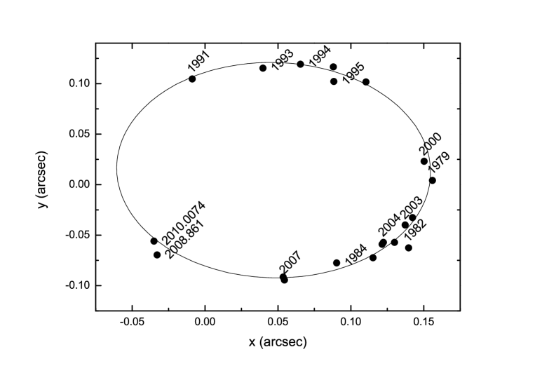
Figure 2: Relative visual orbit of the system HIP12552 showing the epoch of the positional measurements.

5 Synthetic Photometry

As a double-check for the best fit and to present a new synthetic photometrical data of the unseen individual components of the system, we apply the following relation (Maíz Apellániz 2006, 2007):

$$m_{p}[F_{\lambda,s}(\lambda)]=-2.5\log\frac{\int P_{p}(\lambda)F_{\lambda,s}(\lambda)\lambda{\rm d}\lambda}{\int P_{p}(\lambda)F_{\lambda,r}(\lambda)\lambda{\rm d}\lambda}+{\rm ZP}_{p}\,,$$ (9)

to calculate total and individual synthetic magnitudes of the systems, where $m_{p}$ is the synthetic magnitude of the passband $p$, $P_{p}(\lambda)$ is the dimensionless sensitivity function of the passband $p$, $F_{\lambda,s}(\lambda)$ is the synthetic SED of the object and $F_{\lambda,r}(\lambda)$ is the SED of the reference star (Vega). Here the zero points (ZP_p) of Maíz Apellániz (2007) are adopted.

Calculated synthetic magnitudes and color indices of the entire system and individual components of different photometrical systems are shown in Table 6.

Table 6: Synthetic magnitudes and color indices of the system.

Sys.	Filter	Entire	Comp.	Comp.
		$\sigma=\pm 0.03$	a	b
Joh-	$U$	9.22	9.59	10.56
Cou.	$B$	9.11	9.51	10.38
	$V$	8.51	8.95	9.71
	$R$	8.18	8.64	9.36
	$U-B$	0.11	0.08	0.18
	$B-V$	0.60	0.57	0.66
	$V-R$	0.33	0.31	0.36
Ström.	$u$	10.38	10.76	11.70
	$v$	9.44	9.83	10.73
	$b$	8.85	9.27	10.08
	$y$	8.48	8.92	9.68
	$u-v$	0.94	0.93	0.97
	$v-b$	0.59	0.56	0.65
	$b-y$	0.37	0.35	0.40
Tycho	$B_{T}$	9.25	9.65	10.55
	$V_{T}$	8.58	9.01	9.79
	$B_{T}-V_{T}$	0.68	0.64	0.76

Table 7: Comparison between the observational and synthetic magnitudes, colors and magnitude differences of the system Hip 12552.

	Observed a	Synthetic b (This work)
$V_{J}$	$8\hbox{$.\!\!^{m}$}51$	$8\hbox{$.\!\!^{m}$}51\pm 0.03$
$B_{T}$	$9\hbox{$.\!\!^{m}$}24\pm 0.02$	$9\hbox{$.\!\!^{m}$}25\pm 0.03$
$V_{T}$	$8\hbox{$.\!\!^{m}$}59\pm 0.01$	$8\hbox{$.\!\!^{m}$}58\pm 0.03$
$(B-V)_{J}$	$0\hbox{$.\!\!^{m}$}60\pm 0.02$	$0\hbox{$.\!\!^{m}$}60\pm 0.03$
$\triangle m$	$0\hbox{$.\!\!^{m}$}76^{c}\pm 0.03$	$0\hbox{$.\!\!^{m}$}76\pm 0.04$

^a See Table 2

^b See Table 6

^c As the average of all $\Delta m$ using the differnt filters under V-band (see Table 3).

Table 8: Parameters of the components of the system HIP12552.

Parameters	Comp. a	Comp. b
$T_{\rm eff}$ (K)	$6180\pm 50$	$5865\pm 70$
Radius (R⊙)	$1.262\pm 0.08$	$1.006\pm 0.07$
$\log g$	$4.35\pm 0.12$	$4.45\pm 0.14$
$L(L_{\odot})$	$2.09\pm 0.10$	$1.08\pm 0.12$
$M_{bol}$	$3\hbox{$.\!\!^{m}$}95\pm 0.18$	$4\hbox{$.\!\!^{m}$}67\pm 0.19$
$M_{V}$	$4\hbox{$.\!\!^{m}$}07\pm 0.18$	$4\hbox{$.\!\!^{m}$}83\pm 0.19$
Mass ($M_{\odot})^{*}$	$1.17\pm 0.11$	$1.06\pm 0.10$
Sp. Type∗∗	F8	G2
Parallax (mas)	$11.83\pm 1.07$
($\frac{M_{a}+M_{b}}{M_{\odot}}$)∗∗∗	$2.23\pm 0.57$

^∗depending on the evolutionary tracks (Fig. 3),

^∗∗depending on the tables of Lang (1992),

^∗∗∗depending on the orbital solution.

6 Results and Discussion

The synthetic SEDs of the individual component and the system HIP12552 are built using atmospheric modeling and the visual magnitude difference between the two components along with the total observed SED. Least square fitting with weights inversely proportional to the squares of the positional measurement errors is used to modify the orbit of the system. So, the physical and geometrical parameters of HIP12552 are estimated. Fig. 1 shows the best fit of the total synthetic SED to the observed one.

Table 7 shows a comparison between the observational and synthetic magnitudes, colors and magnitudes differences for the system HIP12552. This gives a good indication of the reliability of the estimated parameters of the individual components of the system which are listed in Table 8.

The positions of the system’s components on the evolutionary tracks of Girardi et al. (2000a) (Fig. 3) show that both components with masses $M_{A}=1.20$ and $M_{B}=1.09M_{\odot}$ belong to the main-sequence stars. And their positions on  Girardi et al. (2000a) isochrones for low- and intermediate-mass stars of different metallicities and that of the solar composition [$Z=0.019,Y=0.273$] are shown in Figs  4 &  5, which give an age of the system around $3.0\pm 0.9$ Gy.

Figure 3: The system components on the evolutionary tracks of  Girardi et al. (2000b).

Figure 4: The systems’ components on the isochrones of low- and intermediate-mass, solar composition [$Z$=0.019, $Y$=0.273] stars of  Girardi et al. (2000a).

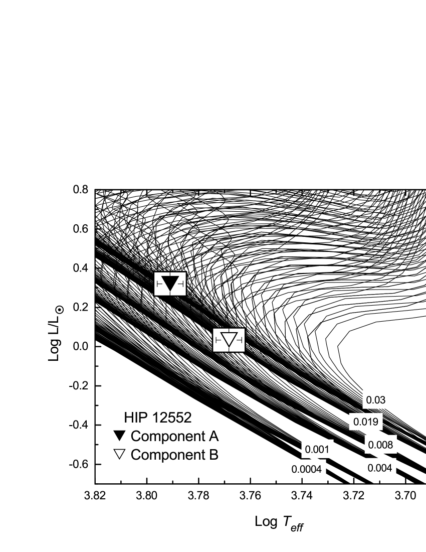
Figure 5: The systems’ components on the isochrones for low- and intermediate-mass stars of different metallicities of  Girardi et al. (2000a).

7 Conclusion

The CVBS COU1511 (HIP12552) is analyzed using Al-Wardat’s complex method for analyzing close visual binary stars, which is based on combining magnitude difference measurements from speckle interferometry, entire spectral energy distribution (SED) from spectrophotometry, atmospheres modeling and orbital analysis to estimate the individual physical and geometrical parameters of the system.

The entire and individual Johnson-Cousin UBVR, Strömgren uvby, and Tycho BV synthetic magnitudes and color indices of the system are calculated. A modified orbit and geometrical elements of the system are introduced and compared with earlier results.

The positions of the two components on the evolutionary tracks and isochrones are shown, their spectral types are estimated as F8 and G1 respectively with the age of $3.0\pm 0.9$ Gy.