Explosive spreading on complex networks: the role of synergy

Abstract

In spite of the vast literature on spreading dynamics on complex networks, the role of local synergy, i.e., the interaction of elements that when combined produce a total effect greater than the sum of the individual elements, has been studied but only for irreversible spreading dynamics. Reversible spreading dynamics are ubiquitous but their interplay with synergy has remained unknown. To fill this knowledge gap, we articulate a model to incorporate local synergistic effect into the classical susceptible-infected-susceptible process, in which the probability for a susceptible node to become infected through an infected neighbor is enhanced when the neighborhood of the latter contains a number of infected nodes. We derive master equations incorporating the synergistic effect, with predictions that agree well with the numerical results. A striking finding is that, when a parameter characterizing the strength of the synergy reinforcement effect is above a critical value, the steady state density of the infected nodes versus the basic transmission rate exhibits an explosively increasing behavior and a hysteresis loop emerges. In fact, increasing the synergy strength can promote the spreading and reduce the invasion and persistence thresholds of the hysteresis loop. A physical understanding of the synergy promoting explosive spreading and the associated hysteresis behavior can be obtained through a mean-field analysis.

I Introduction

Disease or information spreading, a fundamental class of dynamical processes on complex networks Barrat et al. (2008); Castellano et al. (2009); Newman (2010); Pastor-Satorras et al. (2015), has been studied extensively in the past fifteen years Pastor-Satorras and Vespignani (2001); Newman (2002); Zanette (2002); Liu et al. (2003); Barthélemy et al. (2004); Small and Tse (2005); Zhou et al. (2007); Yang et al. (2008); Tang et al. (2009); Gross et al. (2006); Kitsak et al. (2010); Yang et al. (2011); Zhu et al. (2012); Brockmann and Helbing (2013); Gleeson (2013); Boccaletti et al. (2014); Granell et al. (2013); Wang et al. (2014); Liu et al. (2016). Spreading dynamics can be classified into two types: irreversible and reversible. In an irreversible process, once an individual becomes infected, it cannot recover or return to the susceptible state. Or, once an infected node recovers, it is immune to the same virus. Mathematically, irreversible spreading processes can be described by the susceptible-infected (SI), the susceptible-infected-recovered (SIR) Newman (2002), or the susceptible-exposed-infected-recovered (SEIR) model Small and Tse (2005). In contrast, in a reversible process, any node can be infected repeatedly in time, going through a cycle of susceptible and infected states. For example, in the infection process of tuberculosis and gonorrhea, an individual recovering from such a disease can be infected again with the same disease anytime. Mathematically, reversible spreading processes can be described by the susceptible-infected-susceptible (SIS) Pastor-Satorras and Vespignani (2001), the susceptible-infected-recovered-susceptible (SIRS) Bancal and Pastor-Satorras (2010), or the susceptible-exposed-recovered-susceptible (SEIS) model Masuda and Konno (2006). When the complex topology of the underlying network is taken into account, a pioneering result was the vanishing epidemic threshold in scale-free networks with the power-law exponent less than three Pastor-Satorras and Vespignani (2001). Another result is that, for both irreversible and reversible processes described by the classic SIR and SIS models, respectively, the fraction of infected nodes increases with the transmission rate continuously Pastor-Satorras et al. (2015), which can be expected intuitively.

In this paper, we investigate the effect of synergy on reversible spreading dynamics on complex networks. Synergy describes the situation where the interaction of elements that produce a total effect greater than the sum of individual elements when combined, i.e., the phenomenon commonly known as “one plus one is greater than two.” Intuitively, synergy should have a significant effect on spreading dynamics. For example, when a disease begins to spread in the human society, a healthy individual who has a sick friend is likely to be infected with the disease. However, if the sick friend himself or herself has a number of friends with the same disease, the likelihood for the healthy individual to contract the disease would be higher, as (a) the fact that his/her sick friend has sick friends implies that the disease is potentially more contagious, and (b) the healthy individual is likely to have more sick friends. Similarly, in rumor or information spreading over a social network, a number of connected individuals possessing a piece of information make it more believable than just a single individual. Indeed, concrete evidence existed in both biological and social systems where the number of infected neighbors of a pair of infected-susceptible nodes would enhance the transmission rate between them Granovetter (1978); Watts (2002); Lockwood (1988); Ludlam et al. (2012), such as fungal infection in soil-borne plant pathogens Lockwood (1988); Ludlam et al. (2012) where the probability for an infected node to affect its susceptible neighbors depends upon the number of other infected nodes connected to the infected node. In social systems, the synergistic effect was deemed important in phenomena such as the spread of adoption of healthy behavior Centola (2010); Wang et al. (2015), microblogging retweeting Hodas and Lerman (2014), opinion spreading and propagation Castellano et al. (2009); Lu et al. (2011), and animal invasion Murray ; Gordon (2010).

While the classic SIR and SIS models ignore the synergistic effect by assuming that the transmission of infection between a pair of infected-susceptible nodes is independent of the states of their neighbors, there were previous efforts to study the impact of synergy on irreversible spreading dynamics and its interplay with the network topology. In particular, threshold models Granovetter (1978); Watts (2002); Goldenberg et al. (2001) were developed, which take into account neighbors’ synergistic effects on behavior spreading by assuming that a node adopts a behavior only when the number of its adopted neighbors is equal to or exceeds a certain adoption threshold. One result was that, for each node in the network with a fixed adoption threshold, the final adoption size tends to grow continuously and then decreases discontinuously when the mean degree of the network is increased. The SIR model was also generalized to modify the transmission rate between a pair of infected and susceptible nodes according to the synergistic effect Pérez-Reche et al. (2011); Taraskin and Pérez-Reche (2013); Broder-Rodgers et al. (2015), with the finding that it can affect the fraction of the epidemic outbreak, duration and foraging strategy of spreaders. These existing works were exclusively for irreversible spreading dynamics. A systematic study to understand the impact of the synergistic effects on reversible spreading dynamics on complex networks is needed.

The goal of this paper is to investigate, analytically and numerically, the impacts of synergy on reversible spreading dynamics on complex networks. We first generalize the classic SIS model to quantify the effect of the number of infected neighbors connected to an infected node on the transmission rate between it and its susceptible neighbors. To characterize the impact on the steady state of the spreading dynamics, we consider the local nodal environment and derive the master equations (MEs) Lindquist et al. (2011); Gleeson (2011). To gain a physical understanding, we assume that, statistically, nodes with the same degree have the same dynamical characteristics, so the mean-field approximation can be applied. Let $\alpha$ be a parameter characterizing the strength of the synergistic effect. For random regular networks (RRNs), we find that for $\alpha\geq\alpha_{c}$, where $\alpha_{c}$ is a critical value, a hysteresis loop Gross et al. (2006); Yang et al. (2015) appears in which the steady state infected density, denoted by $\rho(\infty)$, increases with the transmission rate $\beta$ but typically exhibits an explosively increasing behavior, in contrast to the typical continuous transition observed in the classic SIS models Pastor-Satorras and Vespignani (2001). For $\alpha<\alpha_{c}$, the hysteresis loop disappears and $\rho(\infty)$ increases with $\beta$ continuously. The phenomena of explosive spreading and hysteresis loop are general in that they also occur for complex networks of different topologies.

II Model

Network model.

The networks in our study are generated from the uncorrelated configuration model Newman (2002) with degree distribution $P(k)$, where the degree-degree correlations can be neglected for large and sparse networks. Nodes in the network correspond to individuals or hosts responsible for spreading, with edges representing the interactions between nodal pairs.

Model of reversible spreading dynamics.

We generalize the classic SIS model to incorporate the synergistic effect into the reversible spreading dynamics — we name it the synergistic SIS spreading model. At any time, each node can only be in one of two states: susceptible (S) or infected (I). An infected node can transmit the disease to its susceptible neighbors. The synergistic mechanism models the role of infected neighbors connected to a transmitter (i.e., an infected node) in enhancing the transmission probability. The synergistic SIS spreading process is illustrated schematically in Fig. 1. Our model differs from the recent one in Ref. Gómez-Gardeñes et al. (2016), which treated the synergistic effect of ignorant individuals attached to a receiver (in ignorant state).

Initially, a fraction $\rho_{0}$ of nodes are chosen as seeds (infected nodes) at random, while the remaining nodes are in the susceptible state. Each infected node can transmit the disease to its susceptible neighbors at the rate

$$p(m,\alpha)=1-(1-\beta)^{1+{\alpha}m},$$ (1)

where $m$ and $\alpha$, respectively, represent the number of the infected neighbors connected to the infected node and the strength of the synergistic effect, and $\beta$ is the basic transmission rate. Equation (1) indicates that, the larger value of $\alpha$ or m, the higher the transmission rate $p(m,\alpha)$ between an infected node and a susceptible neighbor will be. An infected node can recover to being susceptible with probability $\mu$. Our model reduces to the classic SIS model for $\alpha=0$. For $\alpha>0$ ($\alpha<0$), the synergistic effects are constructive (destructive) where the infected neighbors favor (hampers) transmission of the disease to the receivers. In our study, we consider only the constructive synergistic effect, where the infected neighbors of an infected node cooperate with it to spread the disease. In addition, we set $\alpha\leq 1$ so that the synergistic ability of any infected neighbor of the infected node is less than that of itself. This assumption is based on consideration of real situations such as fungal infection in soil-borne plant pathogens where the probability for a susceptible node infected by a direct infected neighbor is always greater than that from an indirect infected neighbor Lockwood (1988); Ludlam et al. (2012).

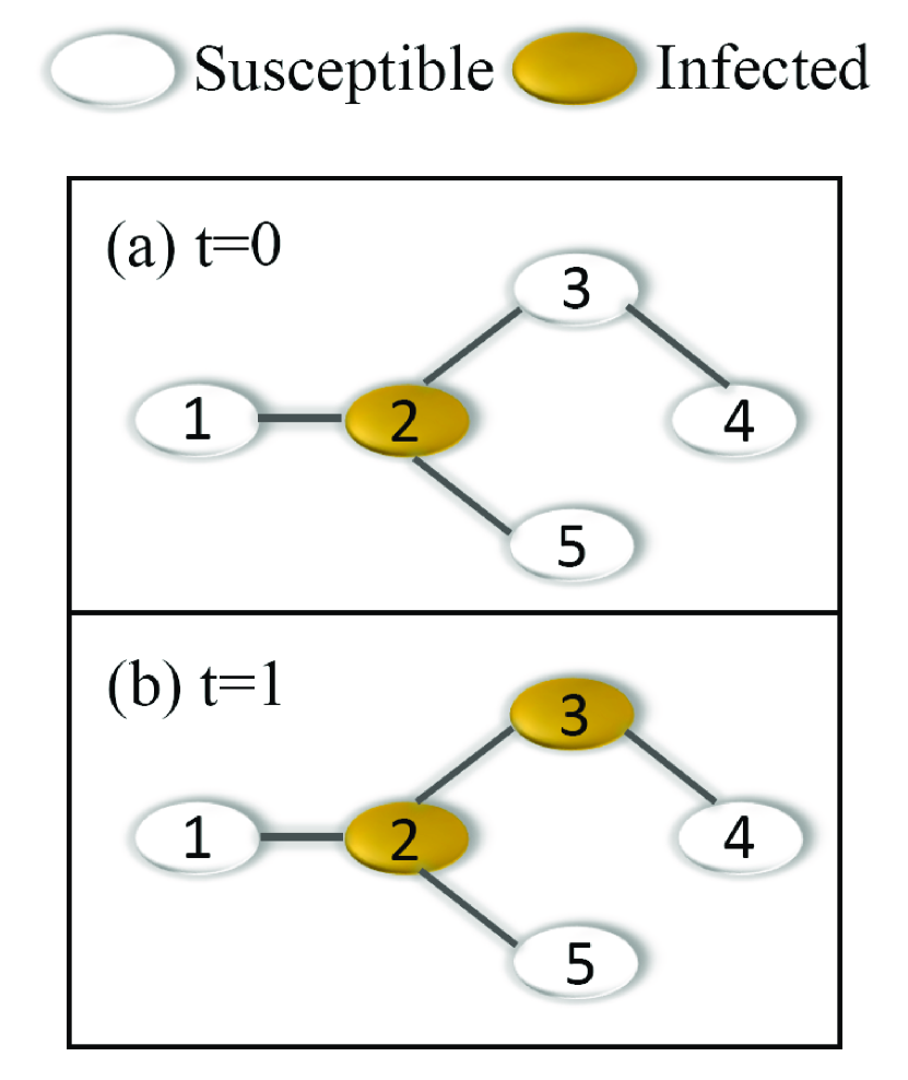
Figure 1: (Color online) Illustration of synergistic SIS spreading process on complex networks. (a) Initially (at $t=0$), node 2 is the seed and the remaining nodes are susceptible. Since there are no infected neighbors connected to node 2, it transmits the disease to one of its susceptible neighbors with probability $p(0,\alpha)=\beta$. (b) Node 3 is infected by node 2 which has not recovered. In this case, both nodes 2 and 3 have an infected neighbor and, at the next time step, they will infect one of their susceptible neighbors with a larger probability $p(1,\alpha)\simeq(1+\alpha)\beta$ due to the synergistic effect.

III Theory

We consider large and sparse networks with negligible degree-degree correlation. We first establish the master equations to describe the synergistic SIS spreading process quantitatively. We then provide an an intuitive understanding of the role of synergy in the spreading dynamics through a mean-filed analysis.

III.1 Master equations

In general, the transmission rate $p(m,\alpha)$ between a pair of infected-susceptible nodes in the synergistic SIS spreading process is determined by the following three factors: (1) the basic transmission rate $\beta$ between the pair of nodes, i.e., the rate in the absence of any synergistic effect, (2) the number of infected neighbors connected to the infected node, and (3) the strength $\alpha$ of the synergistic effect. Because of the strong dynamical correlation among the states of the neighboring nodes leading to the synergistic effect, the approach of master equations Lindquist et al. (2011); Gleeson (2011) can be applied. For convenience, we denote $S_{k,m}$ ($I_{k,m}$) as the k-degree susceptible (infected) node with $m$ infected neighbors and use $s_{k,m}(t)$ and $i_{k,m}(t)$ to express the fractions of $S_{k,m}$ and $I_{k,m}$ nodes at time $t$, respectively. The degree distribution and the average degree of the network are $P_{k}$ and ${\langle k\rangle}=\sum_{k^{\prime}}k^{\prime}P_{k^{\prime}}$, respectively. The fraction of infected nodes with degree $k$ at time $t$ is given by

$$\rho_{k}(t)=\sum_{m=0}^{k}i_{k,m}(t)=1-\sum_{m=0}^{k}s_{k,m}(t),$$

and the total fraction of the infected nodes is $\rho(t)={\langle\rho_{k}(t)\rangle}\equiv{\sum_{k}P_{k}\rho_{k}(t)}$.

To derive the master equations, it is necessary to obtain the probability for $S_{k,m}$ to be infected. Initially, $S_{k,m}$ has $m$ infected neighbors so the probability for one of its infected neighbors to have degree $k^{\prime}$ is $k^{\prime}P_{k^{\prime}}/\langle k\rangle$. This degree $k^{\prime}$ infected neighbor of $S_{k,m}$ may have zero, one, two, or up to $k^{\prime}-1$ infected neighbors. The chance for the degree $k^{\prime}$ infected node to have $n$ infected neighbors is $i_{k^{\prime},n}(t)/i_{k^{\prime}}(t)$, so the probability that it will infect $S_{k,m}$ is

$$\sum_{n=0}^{k^{\prime}-1}\frac{i_{k^{\prime},n}(t)}{i_{k^{\prime}}(t)}p(n,\alpha).$$

Since $S_{k,m}$ has $m$ infected neighbors, the probability of its being infected during time $t+dt$, where $dt$ is an infinitesimally small time interval, can be written as $\pi_{k,m}(t)dt$ with $\pi_{k,m}(t)$ given by

$$\pi_{k,m}(t)=m\sum_{k^{\prime}}\frac{k^{\prime}P_{k^{\prime}}}{\langle k\rangle}\sum_{n=0}^{k^{\prime}-1}\frac{i_{k^{\prime},n}(t)}{i_{k^{\prime}}(t)}p(n,\alpha).$$ (2)

There are three scenarios that can lead to an increase in $s_{k,m}(t)$: (1) recovery of $I_{k,m}$ with probability $\mu$, (2) infection of a susceptible neighbor of $S_{k,m-1}$, and (3) recovery of an infected neighbor of $S_{k,m+1}$. The second (third) scenario corresponds to the situation where an S-S (S-I) edge changes into an S-I (S-S) edge, where an S-S edge connects two susceptible nodes, an S-I edge links a susceptible and an infected nodes, and so on. Denote $\beta^{s}$ as the rate that an S-S edge changes to S-I. We can approximate $\beta^{s}$ as the rate of edges that switch from being S-S to S-I in the time interval $dt$, and the probability $\beta^{s}dt$ is the ratio of the latter to the former. The rate $\beta^{s}$ can thus be approximated as

$$\beta^{s}=\frac{\sum{P_{k}}\sum_{m=0}^{k}(k-m)\pi_{k,m}(t)s_{k,m}(t)}{\sum{P_{k}}\sum_{m=0}^{k}(k-m)s_{k,m}(t)}.$$ (3)

Since the probability for the recovery of an infected node does not depend on its neighbors, the rate at which an S-I edge changes to S-S is $\mu$. Similarly, there are three cases leading to a decrease in $s_{k,m}(t)$: $S_{k,m}$ being infected with probability $\pi_{k,m}$, infection of a susceptible neighbor of $S_{k,m}$ with probability $\beta^{s}$, and recovery of an infected neighbor of $S_{k,m}$ with probability ${\mu}$. We then obtain the time evolution equation of $s_{k,m}(t)$ as

$$\frac{d}{dt}s_{k,m}(t) = {\mu}i_{k,m}(t)+{\beta^{s}}(k-m+1)s_{k,m-1}(t)$$ (4)

$$+ \mu(m+1)s_{k,m+1}(t)$$

$$- [\pi_{k,m}(t)+\beta^{s}(k-m)+{\mu}m]s_{k,m}(t),$$

Analogously, we can derive the time evolution equation of $i_{k,m}(t)$:

$$\frac{d}{dt}i_{k,m}(t) = \pi_{k,m}(t)s_{k,m}(t)+{\beta^{i}}(k-m+1)i_{k,m-1}(t)$$ (5)

$$+ \mu(m+1)i_{k,m+1}(t)$$

$$- [\mu+\beta^{i}(k-m)+{\mu}m]i_{k,m}(t),$$

where $\beta^{i}$ is the rate with which an edge S-I switches to I-I, which can be calculated as

$$\beta^{i}=\frac{\sum{P_{k}}\sum_{m=0}^{k}m\pi_{k,m}(t)s_{k,m}(t)}{\sum{P_{k}}\sum_{m=0}^{k}m{s_{k,m}(t)}}.$$ (6)

If the initially infected nodes are distributed uniformly on the network, the initial conditions of Eqs. (2)-(6) are

$$s_{k,m}(0) = [1-\rho(0)]B_{k,m}[\rho(0)]~{}and$$

$$i_{k,m}(0) = \rho(0)B_{k,m}[\rho(0)],$$

where $B_{k,m}(p)=\binom{k}{m}{p}^{m}{(1-p)}^{k-m}$. Numerically solving Eqs. (2)-(6), we obtain the quantities $i_{k,m}$ and $s_{k,m}$ at any time $t$. The quantity $\rho(\infty)$ can be calculated as $\rho(\infty)=\sum_{k}{P_{k}}\sum_{m=0}^{m=k}i_{k,m}(\infty)$, and we have $s(\infty)=1-\rho(\infty)$. For simplicity, we denote $\rho(\infty)=\rho$.

III.2 Mean-field approximation

To gain physical insights into the role of synergistic effects in spreading dynamics, we develop a mean-field analysis. In particular, we assume that nodes with the same degree exhibit approximately identical dynamical behaviors. The time evolution of the fraction of the degree $k$ infected nodes is then given by

$$\frac{d}{dt}\rho_{k}(t) = [1-\rho_{k}(t)]k$$ (7)

$$\times \sum_{k^{\prime}}\frac{k^{\prime}P_{k^{\prime}}\rho_{k^{\prime}}}{\langle k\rangle}\sum_{m=0}^{k^{\prime}-1}B_{{k^{\prime}-1},m}(w)p(m,\alpha)$$

$$- \mu\rho_{k}(t),$$

where $w=\sum{k{P_{k}}{\rho_{k}}}/{\langle k\rangle}$ is the probability that one end of a randomly chosen edge is infected, $\rho(t)={\sum}P_{k}\rho_{k}(t)$, and the fraction of susceptible nodes at time $t$ is $s(t)=1-\rho(t)$. The steady state of synergistic SIS process in Eq. (7) corresponds to the condition $\frac{d}{dt}\rho_{k}(t)=0$. For degree $k$ we have

$$\rho_{k}(\infty) = \frac{[1-\rho_{k}(\infty)]k}{\mu}$$ (8)

$$\times \sum_{k^{\prime}}\frac{k^{\prime}P_{k^{\prime}}\rho_{k^{\prime}}(\infty)}{\langle k\rangle}\sum_{m=0}^{k^{\prime}-1}B_{{k^{\prime}-1},m}(w)p(m,\alpha),$$

which can be solved analytically for RRNs by approximating $1-{(1-\beta)}^{(1+{\alpha}m)}$ as $\beta(1+{\alpha}m)$ for small $\beta$. We get

$$\rho(\infty) = -\frac{{\alpha}{\beta}k(k-1)}{\mu}{\rho(\infty)}^{3}+\frac{[\alpha{\beta}k(k-1)-{\beta}k]}{\mu}{\rho(\infty)}^{2}$$ (9)

$$+ \frac{{\beta}k}{\mu}{\rho(\infty)},$$

for $t\rightarrow\infty$. Solving Eq. (9), we get the infected density $\rho(\infty)$.

The epidemic threshold is a critical parameter value above which a global epidemic occurs but below which there is no epidemic. Similar to the analysis of the classic SIS spreading dynamics, we can obtain the critical condition from the nontrivial solution of Eq. (9). In particular, the function

$$g[\rho(\infty),\beta,\mu,\alpha] = -\frac{{\alpha}{\beta}k(k-1)}{u}{\rho(\infty)}^{3}$$ (10)

$$+ \frac{[\alpha{\beta}k(k-1)-{\beta}k]}{\mu}{\rho(\infty)}^{2}$$

$$+ \frac{{\beta}k}{\mu}{\rho(\infty)}-{\rho(\infty)},$$

becomes tangent to the horizontal axis at $\rho_{c}(\infty)$, which is the critical infected density in the limit $t\to\infty$. The critical condition is given by

$$\frac{dg[\rho(\infty),\beta,\mu,\alpha]}{d\rho_{\infty}}\rvert_{\rho_{c}(\infty)}=0.$$ (11)

Furthermore, the basic critical transmission rate can be calculated as:

$$\beta_{c}=\frac{\mu}{\Gamma},$$ (12)

where

$$\Gamma=k[1-2(1-(k-1)\alpha)\rho_{c}(\infty)-3(k-1)\alpha{\rho_{c}(\infty)}^{2}].$$

Numerically solving Eqs. (9) and (12), we get the critical transmission rate $\beta_{c}$. For $\alpha=0$, our synergistic SIS spreading model reduces to the classic SIS spreading model, and Eq. (9) has a trivial solution $\rho(\infty)=0$. For $\alpha=0$, Eq. (9) has only one nontrivial solution. We thus see that $\rho(\infty)$ increases with $\beta$ continuously. As shown in Fig. 2(a), the function $g[\rho(\infty),\beta,\mu,\alpha]$ is tangent to the horizontal axis at $\rho(\infty)=0$. Combining Eqs. (9) and (12), we obtain the continuous critical transmission rate $\beta_{c}=\mu/k$ for $\alpha=0$.

For $\alpha>0$ so synergistic effects exist, $\rho({\infty})=0$ is a trivial solution since Eq. (9) is a cubic equation for the variable $\rho(\infty)$ without any constant term. As shown in Fig. 2(b), for a fixed $\alpha>0$ (e.g., $\alpha=0.9$), the number of solutions of Eq. (9) is dependent upon $\beta$, and there exists a critical value of $\beta$ at which Eq. (9) has three roots (fixed points), indicating the occurrence of a saddle-node bifurcation Ott (2002); Strogatz et al. (1994). The bifurcation analysis of Eq. (9) reveals the physically meaningful stable solution of $\theta(\infty)$ will suddenly increase to an alternate outcome. In this case, an explosive growth pattern of $\rho(\infty)$ with $\beta$ emerges. And whether the unstable state stabilizes to an outbreak state [$\rho(\infty)>0$] or an extinct state [$\rho(\infty)=0$] depends on the initial fraction of the infected seeds. As a result, a hysteresis loop emerges Gross et al. (2006); Yang et al. (2015). To distinguish the two thresholds of the hysteresis loop, we denote $\beta_{inv}$ as the invasion threshold corresponding to the trivial solution [$\rho(\infty)=0$] of Eq. (9), associated with which the disease starts with a small initial fraction of the infected seeds, and let $\beta_{per}$ be the persistence threshold corresponding to the nontrivial solution [$\rho_{c}(\infty)>0$] of Eq. (9), at which the disease starts with a higher initial fraction of the infected seeds Gross et al. (2006); Yang et al. (2015). Substituting the trivial solution [$\rho(\infty)=0$] into Eq. (12), we obtain the invasion threshold as

$$\beta_{inv}=\frac{\mu}{k}.$$ (13)

Note that the classic SIS spreading process has the same invasion threshold. We can also solve Eqs. (9) and (12) simultaneously to get the persistence threshold $\beta_{per}$ with $\rho_{c}(\infty)>0$.

We now present an explicit example to understand the relationship between $\rho(\infty)$ and $\beta$. As shown in Fig. 2(b) for $\alpha=0.9$, numerically solving Eqs. (9) and (12) gives the function $g[\rho(\infty),\beta,\gamma,\alpha]$, which becomes tangent to the horizontal axis for $\beta_{inv}=0.01$ or $\beta_{per}\approx 0.0039$. From Fig. 2(b), we see that Eq. (9) has $3$ fixed points when $\beta$ is in the range of ($\beta_{inv},\beta_{per})$. As a result, the steady state infection density depends on $\rho_{0}$. If the disease starts with a small initial fraction of infected seeds, the root with the smallest value [$\rho(\infty)=0$] of Eq. (9) corresponds to the steady state. However, if the disease starts with a large initial fraction of infected seeds, the root with the largest value is the infected density in the steady state. When $\beta$ is smaller than $\beta_{per}$ or larger than $\beta_{inv}$, the initial fraction of infected seeds has no effect on the steady state.

Next, by solving the condition of the saddle-node bifurcation Ott (2002); Strogatz et al. (1994), we can determine the critical value of infected neighbors’ synergy effects $\alpha_{c}$, for $\alpha<\alpha_{c}$, $\rho(\infty)$ increases with $\beta$ continuous, while $\rho(\infty)$ will increase with $\beta$ explosively and the hysteresis appears when $\alpha>\alpha_{c}$. Combing Eqs. (9) and (11) together with the condition

$$\frac{d^{2}g[\rho(\infty),\beta,\mu,\alpha]}{d\rho_{\infty}^{2}}\rvert_{\rho_{c}(\infty)}=0,$$ (14)

we obtain

$$\alpha_{c}=\frac{1}{k-1-3(k-1)\rho_{c}{(\infty)}}.$$ (15)

Combining Eqs. (9), (11) and (15), we get $\alpha_{c}=1/(k-1)$, which is dependent only on the degree of the RRNs.

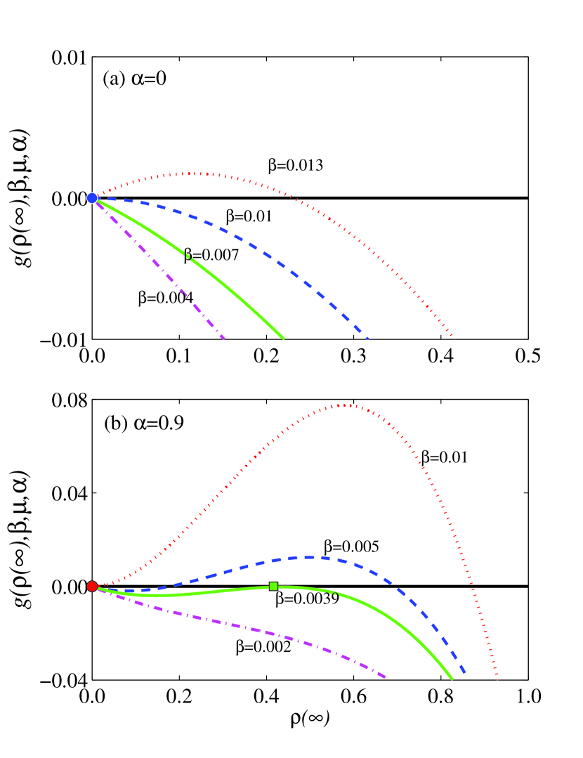
Figure 2: (Color online) Illustration of graphical solution of Eq. (10). For random regular networks with $k=10$, (a) continuously increasing behavior of $\rho(\infty)$ with $\beta$ for $\alpha=0$, (b) explosive change in $\rho(\infty)$ for $\alpha=0.9$. The blue dashed line is tangent to the horizontal axis at $\rho(\infty)=0$ (i.e., the blue circle) in (a). The red circle and green square respectively represent the points of tangency for the red dotted line and green solid line in (b). The recovery rate is $\mu=0.1$.

IV Numerical verification

We perform extensive simulations of synergistic SIS spreading processes on RRNs of size $N=10^{4}$ and degree $k=10$. To calculate the pertinent statistical averages we use 30 network realizations and at least $10^{3}$ independent dynamical realizations for each parameter setting. To be concrete, we take synchronous updating processes Pastor-Satorras et al. (2015) and set the recovery rate as $\mu=0.1$ in all simulations (unless otherwise specified). To obtain the numerical thresholds $\beta_{inv}$ and $\beta_{per}$, we adopt the susceptibility measure Ferreira et al. (2012); Shu et al. (2015):

$$\chi=N\frac{\langle\rho(\infty)^{2}\rangle-{\langle\rho(\infty)\rangle}^{2}}{\langle\rho(\infty)\rangle},$$ (16)

where $\rho(\infty)$ is the steady-state density of infected nodes. In general, $\chi$ exhibits a maximum value at $\beta_{inv}$ and $\beta_{per}$ when the initial fraction of the infected seeds is relatively small and large, respectively. We define $\beta_{inv}^{s}$ ($\beta_{per}^{s}$) as the numerical predictions of invasive (persist) threshold.

Figure 3(a) shows $\rho(\infty)$ versus $\beta$ for $\alpha=0.9$, where the surprising phenomenon of explosive spreading, i.e., $\rho(\infty)$ exhibits an explosive increase as $\beta$ passes through a critical point, can be seen, as predicted [Eqs. (2)-(6), and Eq. (9)]. In fact, there exists a range in $\beta$: [$\beta_{inv}$, $\beta_{per}$], in which the steady state depends on the value of $\rho_{0}$. In particular, the two different steady states correspond to the spreader-free state [$\rho(\infty)=0$] for initially small fraction of infected seeds and the endemic state [$\rho(\infty)>0$] with initially larger fraction of infected nodes, respectively. The coexistence of endemic and spreader-free states, in the form of a hysteresis loop with explosive transitions between the states, is predicted by both theoretical approaches (i.e., the master equations and the mean-field theory), and is observed numerically. Figure 3(b) shows the susceptibility measure $\chi$ versus $\beta$ for the two cases of $\rho_{0}=0.01$ and $\rho_{0}=0.9$. We see that the numerical thresholds $\beta_{inv}^{s}$ and $\beta_{per}^{s}$ determined through $\chi$ match well with the predictions from the master equations, but the mean-field approximation gives only the value of $\beta_{per}^{s}$ correctly. Letting $\triangle\beta$ be the difference between $\beta_{inv}^{s}$ and $\beta_{per}^{s}$ (the width of the hysteresis loop), we find that $\triangle\beta$ increases with $\alpha$, as shown in the inset of Fig. 3(b), indicating that $\beta_{inv}^{s}$ decreases faster than $\beta_{per}^{s}$ as $\alpha$ is increased.

To explain why mean-field approximation can’t accurately predict $\beta_{inv}^{s}$, and to give a qualitative explanation for the explosively increasing behavior of $\rho(\infty)$ with $\beta$, we consider the case where the spreading process starts from a small fraction of infected seeds. Initially, for an infected seed [e.g., node $2$ in Fig. 1(a)], all its neighbors are in the susceptible state. Thus, there is no synergistic effect when this infected node attempts to infect its susceptible neighbors. Once the infected node ($I_{k,0}$) has infected one of its susceptible neighbors [e.g., node $3$ in Fig. 1(a)] successfully, both the originally and newly infected nodes become $I_{k,1}$, leading to a synergistic effect. In this case, if the average number of nodes infected by one seed is larger than 1, an epidemic will occur. In discrete time steps, this average number can be approximately calculated as Shu et al. (2016)

$$R = k\sum_{t=1}^{\infty}[(1-\mu)(1-p(0,\alpha))]^{t-1}p(0,\alpha)$$ (17)

$$+ (k-1)\sum_{t=2}^{\infty}[(1-\mu)(1-p(0,\alpha))]^{t-2}$$

$$\times p(0,\alpha)(1-\mu)[p(1,\alpha)-p(0,\alpha)],$$

where the first term of Eq. (17) represents the basic reproduction number without any synergistic effect, the second term denotes the increment in the basic reproduction number as a result of the synergistic effect due to the newly infected neighbor, if the seed indeed successfully infects a neighbor before its recovery. Letting $R=1$ in Eq. (17), we can approximately calculate the critical invasion threshold as

$$\beta_{inv}^{{}^{\prime}}=\frac{\mu}{k+(k-1)(1-\mu)\alpha+\mu-1}.$$ (18)

As shown in Fig. 4(a), the value of $\beta_{inv}^{{}^{\prime}}$ agrees well with the value of $\beta^{s}_{inv}$. For the case of small initial infected density, the mean-field approximation fails to capture the dynamical correlation. Due to the synergistic effect, even only one end of the I-I edge transmits the disease to its susceptible neighbors, the $I_{k,1}$ node becomes $I_{k,2}$, which has a larger transmission rate than that from the original $I_{k,1}$ node. As the spreading process continues, more susceptible nodes in the neighborhood of the infected node are infected so the $I_{k,2}$ nodes become $I_{k,3}$, $I_{k,3}$ becomes $I_{k,4}$, and so on, leading to a cascading process that results in explosive spreading.

To gain further insights into the cascading phenomenon and the explosive increase of $\rho(\infty)$ with $\beta$ for $\alpha>\alpha_{c}$, we calculate the fraction $i_{m}$ of infected nodes with $m$ ($m=0,1,...,k$) infected neighbors versus time for $\beta$ slightly larger than $\beta_{inv}$ (for $\alpha=0.9$) and $\beta_{c}$ (for $\alpha=0$). For $\alpha<\alpha_{c}$ (e.g., $\alpha=0$), the synergistic SIS spreading is reduced to the classic SIS dynamics. As shown in the inset of Fig. 4(b), for $\beta=0.0114\gtrsim\beta_{c}=0.0112$, $i_{m}$ increases with $t$ slowly and tends to a constant for large time. However, for $\alpha=0.9$, if $\beta=0.0064\gtrsim\beta_{inv}^{s}=0.0062$, $i_{m}$ increases fast initially, reaches a peak at some small value of $m$ (e.g., $m=0,1$), and then decreases rapidly. For larger $m$ values (e.g., $m=3,5$), $i_{m}$ increases later and faster in reaching the peak. These provide an explanation for the continuously and relatively slowly increasing behavior of $\rho(\infty)$ for $\alpha<\alpha_{c}$ and, more importantly, the explosively increasing behavior of $\rho(\infty)$ with $\beta$ for $\alpha>\alpha_{c}$.

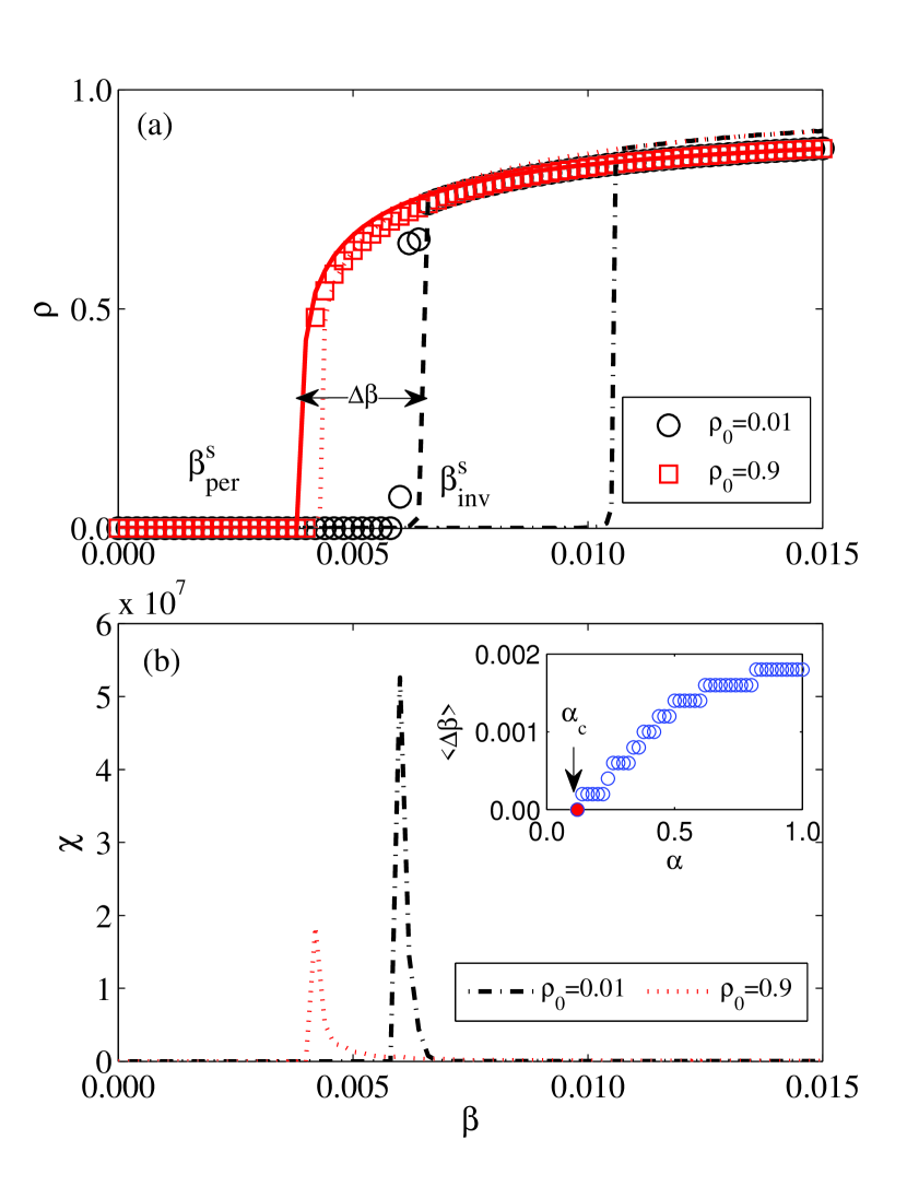
Figure 3: (Color online) Steady state infected density $\rho(\infty)$ and susceptibility measure $\chi$ for random regular networks. (a) The density $\rho(\infty)$ versus $\beta$ for $\alpha=0.9$, where the red squares and black circles are simulation results with initial infected density $\rho_{0}=0.9$ and $\rho_{0}=0.01$, respectively. The red solid and black dashed lines are the results of master equations Eqs. (3)-(6) with the same respective initial seed fractions. The red dotted and black dotted dashed lines are results from the mean-field approximation [Eq. (11)] with the same respective initial seed fractions. The quantities $\beta_{inv}^{s}$ and $\beta_{per}^{s}$ are, respectively, the simulated invasion and persistence thresholds determined via the susceptibility measure. (b) Susceptibility measure $\chi$ versus $\beta$ with the same parameters as in (a). To discern the extremely small value of $\chi$ for $\rho_{0}=0.9$, we plot the dotted line in (b) one thousand times larger than the original values. The inset in (b) shows the width of the hysteresis loop versus $\alpha$. Other parameters are $\mu=0.1$ and $k=10$.

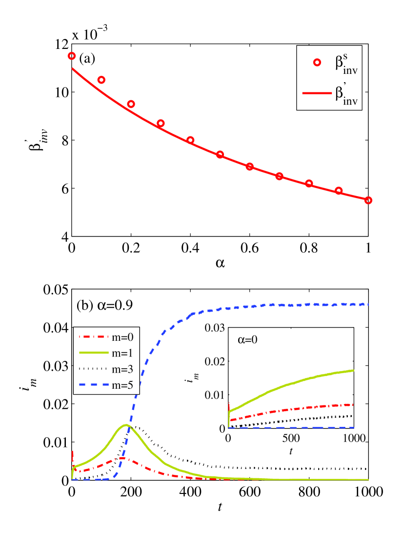
Figure 4: (Color online) Illustration the regime of explosive spreading. (a) Circles indicate the numerical predictions of invasive threshold $\beta^{{}^{\prime}}_{inv}$ in $\alpha$. The solid line shows the transmission rate $\beta$ in Eq. (18). (b) The fraction $i_{m}$ of infected nodes for different numbers of infected neighbors ($m=0,1,3,5$) versus time $t$ when the transmission rate is slightly larger than $\beta_{inv}^{s}$. Panel (b) shows $i_{m}$ versus $t$ for $\alpha=0.9$ and $\beta=0.0064$ ($\beta_{inv}^{s}=0.0062$), where the inset shows the same plot for the classic SIS spreading dynamics for $\beta=0.0114$ ($\beta_{c}=0.0112$). Other parameters are $\rho_{0}=0.01$, $\mu=0.1$ and $k=10$.

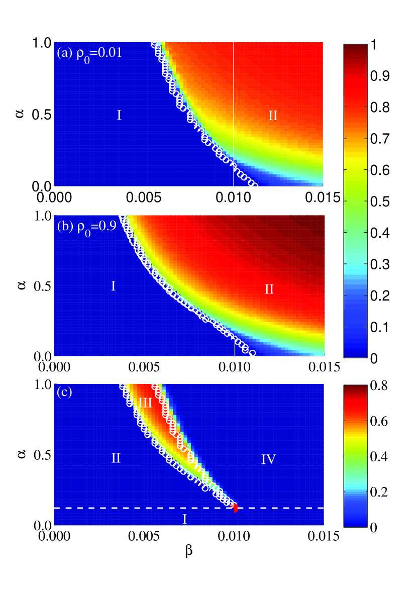
Figure 5: (Color online) Steady state infected density $\rho(\infty)$ and region of hysteresis in the parameter plane ($\beta$, $\alpha$). (a,b) For synergistic SIS spreading dynamics on random regular networks, color-coded values of $\rho(\infty)$ in the parameter plane ($\beta$,$\alpha$) for $\rho_{0}=0.01$ and $\rho_{0}=0.9$, respectively. The numerically obtained invasion threshold $\beta_{inv}^{s}$ and persistence threshold $\beta_{per}^{s}$ (white circles) in (a) and (b), respectively, are determined by the susceptible measure $\chi$, and the corresponding theoretical values (white sold line) are from Eqs. (9) and (12). The persistence threshold predicted by the mean-filed theory matches well with that from simulations, but there is disagreement for the invasion threshold, as shown in (a,b), where I and II denote the parameter regions where the disease becomes extinct and an outbreak occurs, respectively. In (c), the color-coded values represent the difference between the values of $\rho(\infty)$ in (b) and (a). There are four regions: in region I there is no hysteresis loop ($\alpha<\alpha_{c}$), in region III there is a hysteresis behavior, and regines II and IV specify the borders of the hysteresis loop. Other parameters are $\mu=0.1$ and $k=10$.

We further examine the impact of parameters $\beta$ and $\alpha$ on the synergistic SIS spreading dynamics. Figures 5(a) and (b) show the value of $\rho(\infty)$ in the ($\beta$, $\alpha$) plane for $\rho_{0}=0.01$ and $\rho_{0}=0.9$, respectively. In (a), the solid curves represent the analytical predictions of $\beta_{inv}$ versus $\alpha$ obtained from Eq. (13), and the circles display the numerical predictions of $\beta_{inv}^{s}$ determined by the susceptible measure, which increases with $\alpha$. The results in (b) show that the persistence threshold decreases as $\alpha$ is increased. A heuristic explanation for these results is that, due to the synergistic effect, there is an increase in the infection probability $p(m,\alpha)$ between the infected nodes and their susceptible neighbors, thereby reducing the epidemic threshold (e.g., $\beta_{inv}$ and $\beta_{per}$). In Figs. 5(a) and (b), depending on whether the disease becomes extinct or there is an outbreak, we can divide the parameter plane into regions I and II, respectively. For $\beta>\beta_{inv}$ (or $\beta>\beta_{per}$), $\rho(\infty)$ increases with $\alpha$ due to the enhancement in the transmission rate between the infected node and its susceptible neighbors. Since the initial fraction of infected seeds impacts only the steady state associated with the region of the hysteresis loop, we can determine this region by computing the difference between the values of every point ($\beta$,$\alpha$) in Figs. 5(b) and 5(a). As shown in Fig. 5(c), there are four regions. Only when $\alpha$ is larger than a critical value $\alpha_{c}$ [obtained from Eqs. (9), (11) and (15)] will the final density $\rho(\infty)$ increase with $\beta$ explosively (regions II, III, and IV) and a hysteresis loop appears (region III). Otherwise there is no hysteresis (region I). In region II, the disease becomes extinct, but there is an outbreak in region IV.

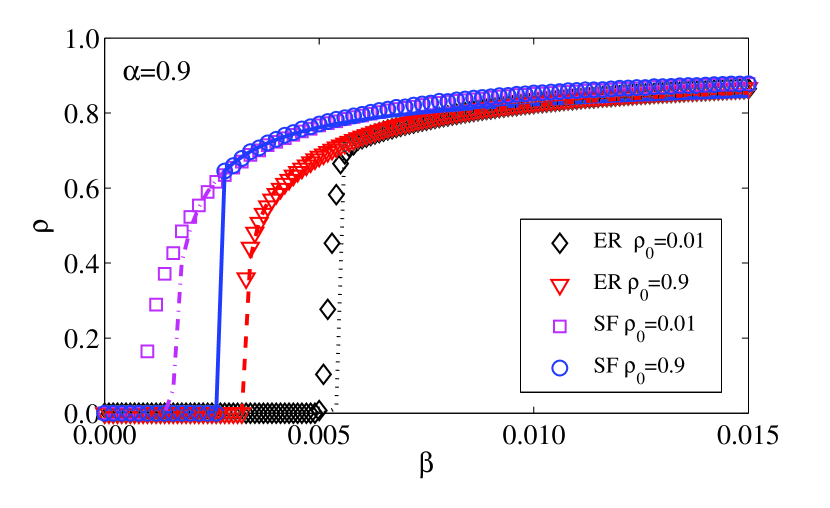
Figure 6: (Color online) Synergistic SIS spreading processes on random and scale-free networks. Steady state density of infected nodes versus $\beta$: where symbols are results from simulation and the corresponding lines are predictions of the master equations Eqs. (3)-(6). The network parameters are $N=10^{4}$ and $\langle k\rangle=10$.

While we focus our study on RRNs for the reason that an understanding of explosive spreading can be obtained, the phenomenon can arise in general complex networks. To demonstrate this, we simulate synergistic spreading dynamics on Erdös-Rényi (ER) random and scale-free networks. Figure 6 shows, for ER networks, an explosive increase in the steady state infection density and a hysteresis loop with the parameter $\beta$. We also investigate the spreading dynamics on scale-free networks Newman (2002) constructed according to the standard configuration model Catanzaro et al. (2005). The degree distribution is $P(k)={\Gamma}k^{-\gamma}$, where $\gamma$ is degree exponent and the coefficient is $\Gamma=1/\sum_{k_{min}}^{k_{max}}k^{-\gamma}$ with the minimum degree $k_{min}=3$, maximum degree $k_{max}{\sim}N^{1/(\gamma-1)}$ and $\gamma=3.0$. The phenomena of explosive spreading and hysteresis loop are presented, as shown in Fig. 6.

V Discussion

Synergy is a ubiquitous phenomenon in biological and social systems, and one is naturally curious about its effect on spreading dynamics on networks. There were previous works on synergistic irreversible spreading dynamics, and the goals of this paper are to construct and analyze a generic model for synergistic reversible spreading, where the effect of synergy is taken into account through enhancement in the transmission rate between an infected node and its susceptible neighbors. There are two factors determining the synergistic effect: the number of infected neighbors connected to the infected node that is to transmit the disease to one of its susceptible neighbors and the strength of the synergistic reinforcement effect. For RRNs, the synergistic reversible spreading dynamics can be treated analytically by using the approach of master equations, as well as a mean field approximation. Qualitatively, we find that synergy promotes spreading. The manner by which spreading is enhanced is, however, quite striking. In particular, if the strength is above a critical value that is solely determined by the degree of the network, there is an explosive outbreak of the disease in that the steady state infection density increases abruptly and drastically as the basic transmission rate passes through a critical value. Associated with the explosive behavior is a hysteresis loop whereas, if the transmission rate is reduced through a different threshold, the final infected population collapses to zero. All these results have been obtained both analytically and numerically. While the analysis is feasible for RRNs, numerically we find that a similar explosive behavior occurs for general complex networks with a random or a scale-free topology.

The main contributions of our work are thus the discovery of synergy induced explosive outbreak for reversible spreading dynamics, and a qualitative and quantitative understanding of the phenomenon. A number of questions still remain. For example, the effects of network structural characteristics such as clustering Serrano and Boguñá (2006); Newman (2009); Cui et al. (2012), community Girvan and Newman (2002); Fortunato (2010); Gong et al. (2013), and core-periphery Borgatti and Everett (2000); Holme (2005); Liu et al. (2015); Verma et al. (2016) on synergistic spreading dynamics need to be studied. The approach of master equations needs to be improved beyond random regular networks. Finally, the study needs to be extended to more realistic networks such as multiplex networks Boccaletti et al. (2014); Wang et al. (2014); Liu et al. (2016); Kivelä et al. (2014), or temporal networks Holme and Saramäki (2012); Barrat et al. (2013); Moinet et al. (2015).