Analysis of the Lepton Mixing Matrix in the Two Higgs Doublet Model

Abstract

In the theoretical framework of Two Higgs Doublet Model (2HDM) plus three right-handed neutrinos we consider a universal treatment for the mass matrices, aside from that the active neutrinos acquire their small mass through the type-I seesaw mechanism. Then, as long as a matrix with four-zero texture is used to represent the right-handed neutrinos and Yukawa matrices, we obtain a unified treatment where all fermion mass matrices have four-zero texture. We obtain analytical and explicit expressions for the lepton flavour mixing matrix PMNS in terms of fermion masses and parameters associated with the 2HDM-III. Further, we compare these expressions of the PMNS matrix with the most up to date values of masses and mixing in the lepton sector, via a likelihood test $\chi^{2}$. We find that the analytical expressions that we derived reproduce remarkably well the most recent experimental data of neutrino oscillations.

Keywords: Neutrinos, Seesaw, PMNS matrix, 2HDM-III.

I Introduction                                                                                                                      

Although highly successful in terms of its phenomenological predictions, the Standard Model (SM) of electroweak interactions seems incomplete from a theoretical view. In its present form, it is unable to predict the masses of fermions (leptons and quarks), or explain why there are several families of such particles. One of the most interesting phenomena is presented by the neutrino mixing, a phenomenon known as neutrino oscillation. In concordance with the recent work focus on neutrino physics Capozzi et al. (2016), neutrino mass scale, corresponding Dirac or Majorana kind of fermion, and the source of Charge-Parity (CP) violation are unsolved questions. For that, see the experimental results concerning KamLAND (KL) reactor neutrinos Gando et al. (2011, 2013); Seo (2015), with respect to the expectations from reference Huber-Müller (HM) spectra Gando et al. (2011, 2013). In each of the current high-statistics short-baseline(SBL) reactor experiments RENO Seo (2015); Choi et al. (2015), Double Chooz Abe et al. (2014) and Daya Bay An et al. (2015). In general, if neutrinos are massive particles and their masses are non-degenerate, it is impossible to find a flavour basis in which the coincidence between flavour and mass eigenstates holds both for charged leptons and for neutrinos. Hence, the phenomenon of leptonic flavour mixing is naturally appear between three charged leptons and three massive neutrinos. If there exist irremovable phase factors in the Yukawa interactions, the CP violation will naturally appear both in the quark and lepton sector.

In this context, the flavour and mass generation are two concepts strongly intertwined. To know the flavour dynamic in models beyond the SM, we need to understand the flavour mechanism and mass generation arising in the standard theory. In this theory, the Yukawa matrices are of great interest because the values of its elements define to the fermion masses, as well as its phases factors are related with the CP violation through the mixing matrix.

Moreover, the flavour changing currents arise from the not simultaneous diagonalization of Higgs and Yukawa matrices. Particularly, we will study the flavour dynamics through Yukawa matrices in the 2HDM-III (see therein references related with this model in Ref. Félix-Beltrán et al. (2015)), which into the processes comes with flavour violation through Higgs states, that is, it allows to appear the Flavour Changing Neutral Currents (FCNC) mediated by Higgs fields.

Other models like the 2HDM-III allow the FCNC Atwood, Reina, and Soni (1997); Krawczyk and Sokolowska (2007). The difference between these models is in the Yukawa structure and symmetries of the Higgs sector as well as the possible appearance of new sources of CP violation. In this work, the Higgs potential preserves the CP symmetry with the Hermitian Yukawa matrices. 2HDM-III predicts three neutral states and a pair of charged states: $H^{0}_{1,2,3}$ and $H^{\pm}_{1,2}$ Krawczyk (2006).

In 2HDM-III, FCNC are kept under control by imposing some texture of Yukawa matrices that reproduce the observed fermion masses and mixing angles Deppisch (2013). Using texture forms allows for a direct relation between the Yukawa matrix elements and the parameters related with the decay widths and cross section without losing the terms proportional to the light fermions masses. Specifically, considering a four-zero texture Yukawa matrix, one obtains in a natural way the Cheng-Sher ansatz for couplings flavour mix, which is widely used in the literature, where flavoured couplings are considered proportional to the involved fermion masses Félix-Beltrán et al. (2015); Dorsner and Barr (2002).

This work is realized in the frame of 2HDM-III, considering a hybrid treatment of the neutral leptonic sector through type-I seesaw mechanism. Moreover, a four-zero texture ansatz for Dirac and Majorana neutrino mass matrices, left and right-handed neutrinos respectively. We perform a statistical analysis of neutrino mixing angles using the likelihood test $\chi^{2}$.

II  The 2HDM and seesaw mechanism                                                                                   

In order to make a minimal extension of 2HDM by introducing right-handed neutrinos, we need to consider six neutrino fields; three left-handed neutrinos $\nu_{L}=\left(\nu_{eL},\nu_{\mu L},\nu_{\tau L}\right)^{\top}$ and three right-handed neutrinos $N_{R}=\left(N_{1R},N_{2R},N_{3R}\right)$. Where only the left-handed fields take part in the electroweak interactions. In context of Two Higgs Doublet Model plus massive neutrinos, 2HDM+3$\nu$, for Dirac leptons the Lagrangian of Yukawa interactions has the form:

$${\cal L}_{Y}=\sum_{k=1}^{2}\left(\,\mathbf{Y}_{k}^{\nu}\,\bar{L}\,\tilde{\Phi}_{k}\,N_{R}+\mathbf{Y}_{k}^{l}\,\bar{L}\,\Phi_{k}\,l_{R}\,\right)+\textrm{H.c.}\,,$$ (1)

where $L=(\nu_{l},l^{-})^{\top}_{L}$ is the left-handed doublet of $SU(2)$, the index $l$ represents the charged leptons. The $\Phi_{k}=(\phi_{k}^{+},\phi_{k}^{0})^{\top}$ denotes the Higgs doublets with $\tilde{\Phi}_{k}=i\sigma_{2}\Phi_{k}^{*}$. Finally, the $\mathbf{Y}_{k}^{j}$ with $j=l,\nu$, are the complex Yukawa $3\times 3$ matrices. In flavour space, the Dirac fermion mass matrix can be written as:

$$\mathbf{M}_{j}=\frac{1}{\sqrt{2}}\left(\,v_{1}\,\mathbf{Y}_{1}^{j}+v_{2}\,\mathbf{Y}_{2}^{j}\,\right),$$ (2)

where $v_{1,2}$ are the vacuum expectation values (vev) associated with each of the Higgs doublets. In addition, these matrices can be diagonalized through a unitary transformation $\mathbf{U}$, such that:

$$\mathbf{U}_{j\,L}\,\mathbf{M}_{j}\,\mathbf{U}_{j\,R}^{\dagger}=\frac{1}{\sqrt{2}}\left(v_{1}\,\mathbf{\tilde{Y}}_{1}^{j}+v_{2}\,\mathbf{\tilde{Y}}_{2}^{j}\right)=\textrm{diag}\{\,m_{j1},\,m_{j2},\,m_{j3}\}$$ (3)

where $\tilde{\bf Y}_{k}^{f}={\bf U}_{jL}{\bf Y}_{k}^{j}{\bf U}_{jR}^{\dagger}$ are the Yukawa matrices in the mass basis, which give us the shape of Fermion-Fermion-Higgs couplings.

Here we consider that active neutrinos acquire their small mass through some seesaw mechanism. Hence, it is possible to write out the following hybrid mass term which involves both Dirac and Majorana neutrinos

$${\cal L}^{D+M}=-\overline{\nu}_{L}\,{\bf M}_{D}\,N_{R}-\frac{1}{2}\overline{\nu}_{L}\,{\bf M}_{L}\,\left(\nu_{L}\right)^{c}-\frac{1}{2}\overline{\left(N_{R}\right)^{c}}{\bf M}_{R}N_{R}+\textrm{H.c.}\;.$$ (4)

In the above expression $M_{D}$ is the Dirac neutrino mass matrix, while $M_{L}$ and $M_{R}$ are symmetric mass matrices because the corresponding mass terms are of the Majorana type. In this case the lepton number $L$ is not conserved. In order to diagonalize the hybrid Lagrangian, Eq. (4), we can begin by rewriting to ${\cal L}^{D+M}$ as follows:

$${\cal L}^{D+M}=-\frac{1}{2}\bar{n}_{L}{\bf M}^{D+M}\left(n_{L}\right)^{c}+\textrm{H.c.}\;,$$ (5)

where $n_{L}=\left(\,\nu_{L}\,,\,\left(N_{R}\right)^{c}\,\right)$ and

$${\bf M}^{D+M}=\left(\begin{array}[]{ccc}\mathbf{M}_{L}&\mathbf{M}_{D}\\ \\ \mathbf{M}_{D}^{\top}&\mathbf{M}_{R}\end{array}\right)$$ (6)

is a $6\times 6$ complex symmetric matrix and can be presented in its diagonal form as:

$$\mathbf{m}={\mathbf{U}}^{\top}{\mathbf{M}}^{D+M}\mathbf{U}=\textrm{diag}\{\lambda_{1},\lambda_{2}\},$$ (7)

where $\mathbf{U}$ is a $6\times 6$ unitary matrix. In the case that neutrino mass matrices satisfy the following hierarchy condition $\mathbf{M}_{R}\gg\mathbf{M}_{D}\gg\mathbf{M}_{L}$, we obtain that eigenvalues of ${\mathbf{M}}^{D+M}$ matrix take the form:

$$\lambda_{1}\approx{\bf M}_{R}\quad\textrm{and}\quad\lambda_{2}\approx{\bf M}_{L}-\mathbf{M}_{D}{\bf M}_{R}^{-1}\mathbf{M}_{D}^{\top}.$$ (8)

The previous expression is known as type-(I+II) seesaw mechanism, and it is just the effective mass matrix of three active neutrinos.

III  Fermion mass matrices                                                                                                     

In general, the Dirac fermion mass matrix has an arbitrary shape, while the right-handed neutrino mass matrix must be symmetric, since these latter are Majorana particles. In particular, in this work we consider that, respectively, the Dirac fermion and right-handed neutrino mass matrices are represented with an Hermitian and complex symmetric matrix with a four-zero texture shape. The explicit form of these matrices are the following

$$\mathbf{M}_{j}={\bf P}_{j}^{\dagger}\,\overline{\bf M}_{j}\,{\bf P}_{j}=\begin{pmatrix}\vspace{2mm}1&0&0\\ \vspace{2mm}0&e^{-i\theta_{C}}&0\\ \vspace{2mm}0&0&e^{-i\left(\theta_{B}+\theta_{C}\right)}\end{pmatrix}\begin{pmatrix}\vspace{2mm}0&\left|C_{j}\right|&0\\ \vspace{2mm}\left|C_{j}\right|&\widetilde{B}_{j}&\left|B_{j}\right|\\ \vspace{2mm}0&\left|B_{j}\right|&A_{j}\end{pmatrix}\begin{pmatrix}\vspace{2mm}1&0&0\\ \vspace{2mm}0&e^{i\theta_{C}}&0\\ \vspace{2mm}0&0&e^{i\left(\theta_{B}+\theta_{C}\right)}\end{pmatrix}\qquad\textrm{and}\qquad\mathbf{M}_{R}=\begin{pmatrix}0&c&0\\ c&\widetilde{b}&b\\ 0&b&a\end{pmatrix},$$ (9)

where $\theta_{B}\equiv\arg\left\{B_{j}\right\}$ and $\theta_{C}\equiv\arg\left\{C_{j}\right\}$. From the expressions for the Dirac fermion mass matrix given in Eqs. (2) and (9), we obtain that $\mathbf{Y}_{k}^{j}$ Yukawa matrices also have a shape with four-zero texture, as shown below

$$\mathbf{M}_{j}=\begin{pmatrix}\vspace{1mm}0&C_{j}&0\\ \vspace{1mm}C_{j}^{\ast}&\widetilde{B}_{j}&B_{j}\\ 0&B_{j}^{\ast}&A_{j}\end{pmatrix}=\frac{v\cos{\beta}}{\sqrt{2}}\left[\begin{pmatrix}\vspace{2mm}0&C^{j}_{1}&0\\ \vspace{2mm}C^{j\,\ast}_{1}&\widetilde{B}^{j}_{1}&B^{j}_{1}\\ \vspace{2mm}0&B^{j\,\ast}_{1}&A^{j}_{1}\end{pmatrix}+\tan{\beta}\begin{pmatrix}\vspace{2mm}0&C^{j}_{2}&0\\ \vspace{2mm}C^{j\,\ast}_{2}&\widetilde{B}^{j}_{2}&B^{j}_{2}\\ \vspace{2mm}0&B^{j\,\ast}_{2}&A^{j}_{2}\end{pmatrix}\right]\,,$$ (10)

where $\tan\beta=v_{2}/v_{1}$ and $v^{2}=v_{1}^{2}+v_{2}^{2}=(246.22~{}\textrm{GeV})^{2}$.

Additionally, here we consider that the left-handed neutrinos acquire their small mass through the type-I seesaw mechanism, which is defined as: ${\bf M}_{\nu_{L}}={\bf M}_{D}\;{\bf M}_{R}^{-1}\;{\bf M}_{D}^{\top}$. So, from the mass matrices given in Eq. (9) the $\mathbf{M}_{\nu_{L}}$ matrix takes the following explicit form

$$\mathbf{M}_{\nu_{L}}=\mathbf{K}\,\overline{\mathbf{M}}_{\nu_{L}}\,\mathbf{K}=\begin{pmatrix}\vspace{2mm}1&0&0\\ \vspace{2mm}0&e^{i\varphi_{B}/2}&0\\ \vspace{2mm}0&0&e^{i\varphi_{A}/2}\end{pmatrix}\begin{pmatrix}\vspace{2mm}0&\left|C_{\nu_{L}}\right|&0\\ \vspace{2mm}\left|C_{\nu_{L}}\right|&\left|\widetilde{B}_{\nu_{L}}\right|&\left|B_{\nu_{L}}\right|\\ \vspace{2mm}0&\left|B_{\nu_{L}}\right|&\left|A_{\nu_{L}}\right|\end{pmatrix}\begin{pmatrix}\vspace{2mm}1&0&0\\ \vspace{2mm}0&e^{i\varphi_{B}/2}&0\\ \vspace{2mm}0&0&e^{i\varphi_{A}/2}\end{pmatrix},$$ (11)

where

$$\begin{array}[]{l}\vspace{2mm}A_{\nu_{L}}=\frac{A_{D}^{2}}{a},\quad B_{\nu_{L}}=\frac{B_{D}^{\ast}C_{D}^{\ast}}{c}+A_{D}\left(\frac{B_{D}}{a}-\frac{bC_{D}^{\ast}}{ac}\right),\quad C_{\nu_{L}}=\frac{\left|C_{D}\right|^{2}}{c},\\ \widetilde{B}_{\nu_{L}}=\left(-\frac{bB_{D}}{ac}-\frac{(a\widetilde{b}-b^{2})C_{D}^{\ast}}{ac^{2}}+\frac{\widetilde{B}_{D}}{c}\right)C_{D}^{\ast}+\frac{\widetilde{B}_{D}C_{D}^{\ast}}{c}+B_{D}\left(\frac{B_{D}}{a}-\frac{bC_{D}^{\ast}}{ac}\right).\end{array}$$ (12)

The elements of diagonal phase matrix $\mathbf{K}$ are defined as $\varphi_{A}\equiv\arg\left\{A_{\nu_{L}}\right\}$ and $\varphi_{B}\equiv\arg\left\{\widetilde{B}_{\nu_{L}}\right\}$. Also, the phase factors of $\mathbf{M}_{\nu_{L}}$ matrix must satisfy the conditions $2\arg\left\{C_{\nu_{L}}\right\}=\arg\left\{\widetilde{B}_{\nu_{L}}\right\}$ and $2\arg\left\{B_{\nu_{L}}\right\}=\arg\left\{A_{\nu_{L}}\right\}+\arg\left\{\widetilde{B}_{\nu_{L}}\right\}$.

The real symmetric mass matrix $\overline{\bf M}_{f}$, with $f=u,d,l,\nu_{L}$, may be brought to diagonal form by means of an orthogonal transformation,

$$\overline{\bf M}_{f}={\bf O}_{f}\;\textrm{diag}\left(\lambda_{f1}\;,\lambda_{f2}\;,\lambda_{f3}\;\right)\;{\bf O}_{f}^{\top}$$ (13)

where the $\lambda_{f}$’s are the eigenvalues of ${\bf M}_{f}$ matrix and ${\bf O}_{f}$ is a real orthogonal matrix. Hence, the invariants of $\overline{\bf M}_{f}$ matrix are

$$\begin{array}[]{l}\vspace{2mm}\textrm{Tr}\left\{\overline{\mathbf{M}}_{f}\right\}=A_{f}+\widetilde{B}_{f}=\lambda_{f1}+\lambda_{f2}+\lambda_{f3},\\ \vspace{2mm}\textrm{Det}\left\{\overline{\mathbf{M}}_{f}\right\}=-A_{f}\left|C_{f}\right|^{2}=\lambda_{f1}\lambda_{f2}\lambda_{f3},\\ \vspace{2mm}\chi\left\{\overline{\mathbf{M}}_{f}\right\}=\frac{1}{2}\left(\textrm{Tr}\left\{\overline{\mathbf{M}}_{f}^{2}\right\}-\textrm{Tr}\left\{\overline{\mathbf{M}}_{f}\right\}^{2}\right)=-A_{f}\widetilde{B}_{f}+|B_{f}|^{2}+|C_{f}|^{2}=-\lambda_{f1}\lambda_{f2}-\lambda_{f1}\lambda_{f3}-\lambda_{f2}\lambda_{f3}.\end{array}$$ (14)

From the above expressions we may express the elements of $\overline{\bf M}_{f}$ matrices in terms of its mass eigenvalues. However, they are unable to give us information about the possible hierarchy in the mass spectrum. Therefore, a matrix with the four-zero texture shape allows to have a normal or inverted hierarchy in the fermionic masses. This latter hierarchy only is possible for the left-handed neutrino masses.

III.1  The mixing matrix as function of fermion masses                                                                

After obtaining the neutrino mass matrix through the type-I seesaw mechanism, let this matrix diagonalize in the context of two different scenarios, which depend on the mass hierarchy imposed on the neutrino mass matrix: Normal Hierarchy (NH) and Inverted Hierarchy (IH).

Normal hierarchy

The NH in the eigenvalues of $\mathbf{M}_{f}$ matrix is defined as $\lambda_{i3}>\lambda_{i2}>\lambda_{i1}$. Hence, the mass matrix parameters in terms of mass eigenvalues and the $(3,3)$ mass matrix entry, take the form

$$\widetilde{B}_{f} = \lambda_{f1}+\lambda_{f2}+\lambda_{f3}-A_{f},$$ (15)

$$\left|C_{f}\right|^{2} = -\frac{\lambda_{f1}\lambda_{f2}\lambda_{f3}}{A_{f}},$$ (16)

$$\left|B_{f}\right|^{2} = \frac{(\lambda_{f3}-A_{f})(A_{f}-\lambda_{f1})(A_{f}-\lambda_{f2})}{A_{f}}.$$ (17)

According with the results, we have to take $\lambda_{fj}=-\left|\lambda_{fj}\right|$ with $j=1,2,3$ such that

$$\begin{array}[]{lcl}\vspace{2mm}\lambda_{f3}>A_{i}>\lambda_{f2}&\textrm{for}&\lambda_{f1}=-\left|\lambda_{f1}\right|,\\ \vspace{2mm}\lambda_{f3}>A_{i}>\lambda_{f1}&\textrm{for}&\lambda_{f2}=-\left|\lambda_{f2}\right|,\\ \vspace{2mm}\lambda_{f2}>A_{i}>\lambda_{f1}&\textrm{for}&\lambda_{f3}=-\left|\lambda_{f3}\right|.\end{array}$$ (18)

In case of the charged leptons: $\lambda_{l1}=m_{e},\;\lambda_{l2}=m_{\mu},\;\lambda_{l3}=m_{\tau}$. The NH is evident by defining the adimensional parameters $\widetilde{M}_{f}\equiv M_{f}/\lambda_{f3}$. Also, assuming this hierarchical ansatz, the heaviest particle is placed in the $(3,3)$ mass matrix entry. Then, it is assumed that the parameter $a_{f}=A_{f}/\lambda_{f3}$ is very close to 1, therefore one can define $a_{f}\equiv 1-\delta_{f}$, and the mass matrix takes the expression

$$\widetilde{M}_{f} = \begin{pmatrix}0&\sqrt{\frac{\widetilde{\lambda}_{f1}\,\widetilde{\lambda}_{f2}}{1-\delta_{f}}}&0\\ \sqrt{\frac{\widetilde{\lambda}_{f1}\,\widetilde{\lambda}_{f2}}{1-\delta_{f}}}&\widetilde{\lambda}_{f1}-\widetilde{\lambda}_{f2}+\delta_{i}&\sqrt{\frac{\delta_{f}}{1-\delta_{f}}\xi_{f1}\xi_{f2}}\\ 0&\sqrt{\frac{\delta_{f}}{1-\delta_{f}}\xi_{f1}\xi_{f2}}&1-\delta_{f}\end{pmatrix},$$ (19)

where

$$\xi_{f1}=\left(1-\delta_{i}-\widetilde{\lambda}_{f1}\right)\quad\textrm{and}\quad\xi_{f2}=\left(1-\delta_{i}+\widetilde{\lambda}_{f2}\right),$$ (20)

with $\widetilde{\lambda}_{f1}=\lambda_{f1}/\lambda_{f3}$ and $\widetilde{\lambda}_{f2}=\left|\lambda_{f2}\right|/\lambda_{f3}$.

Inverted hierarchy

For an inverted hierarchy (IH), the relation between the eigenvalues is $\lambda_{f2}>\lambda_{f1}>\lambda_{f3}$. Analogous to NH, the mass matrix parameters are expressed in terms of eigenvalues as

$$\widetilde{B}_{f} = \lambda_{f1}+\lambda_{f2}+\lambda_{f3}-A_{f},$$ (21)

$$\left|C_{f}\right|^{2} = -\frac{\lambda_{f1}\lambda_{f2}\lambda_{f3}}{A_{f}},$$ (22)

$$\left|B_{f}\right|^{2} = \frac{(A_{f}-\lambda_{f3})(A_{f}-\lambda_{f1})(\lambda_{f2}-A_{f})}{A_{f}}.$$ (23)

According with the results, we have to take $\lambda_{fj}=-|\lambda_{fj}|$ with $j=1,2,3$ such that

$$\begin{array}[]{lcl}\vspace{2mm}\lambda_{f2}>A_{i}>\lambda_{f3}&\textrm{for}&\lambda_{f1}=-\left|\lambda_{f1}\right|,\\ \vspace{2mm}\lambda_{f1}>A_{i}>\lambda_{f3}&\textrm{for}&\lambda_{f2}=-\left|\lambda_{f2}\right|,\\ \vspace{2mm}\lambda_{f2}>A_{i}>\lambda_{f1}&\textrm{for}&\lambda_{f3}=-\left|\lambda_{f3}\right|.\end{array}$$ (24)

For neutrinos: $\lambda_{\nu_{L1}}=m_{\nu{{}_{1}}}$, $\lambda_{\nu_{L2}}=m_{\nu{{}_{2}}}$, $\lambda_{\nu_{L3}}=m_{\nu{{}_{3}}}$; and for the charged leptons: $\lambda_{l1}=m_{e}$, $\lambda_{l2}=m_{\mu}$, $\lambda_{l3}=m_{\tau}$. For this hierarchy, the mass matrix is

$$\widetilde{M}_{i}=\begin{pmatrix}0&\sqrt{\frac{\widetilde{\lambda}_{f1}\,\widetilde{\lambda}_{f3}}{1-\delta_{f}}}&0\\ \sqrt{\frac{\widetilde{\lambda}_{f1}\,\widetilde{\lambda}_{f3}}{1-\delta_{f}}}&-\widetilde{\lambda}_{f1}+\widetilde{\lambda}_{f3}+\delta_{f}&\sqrt{\frac{\delta_{f}}{1-\delta_{f}}\xi_{f1}\xi_{f3}}\\ 0&\sqrt{\frac{\delta_{f}}{1-\delta_{f}}\xi_{f1}\xi_{f3}}&1-\delta_{f}\end{pmatrix}$$ (25)

where

$$\xi_{f1}=\left(1-\delta_{f}+\widetilde{\lambda}_{f1}\right),\quad\textrm{and}\quad\xi_{f3}=\left(1-\delta_{f}-\widetilde{\lambda}_{f3}\right),$$ (26)

with $\widetilde{\lambda}_{f3}=\lambda_{f3}/\lambda_{f2}$ and $\widetilde{\lambda}_{f1}=\left|\lambda_{f1}\right|/\lambda_{f2}$.

For a normal [inverted] hierarchy in the neutrino mass spectrum the real orthogonal matrix that diagonalized the fermion mass matrix with four-zero texture, in terms of fermion masses has the form:

$${\bf O}_{f}=\left(\begin{array}[]{ccc}\vspace{2mm}\sqrt{\frac{\widetilde{m}_{f2[1]}\,\xi_{f1[3]}}{{\cal D}_{f1[3]}}}&-\sqrt{\frac{\widetilde{m}_{f1[3]}\,\xi_{f2[1]}}{{\cal D}_{f2[1]}}}&\sqrt{\frac{\widetilde{m}_{f1[3]}\,\widetilde{m}_{f2[1]}\,\delta_{f}}{{\cal D}_{f3[2]}}}\\ \vspace{2mm}\sqrt{\frac{\widetilde{m}_{f1[3]}\,\left(1-\delta_{f}\right)\,\xi_{f1[3]}}{{\cal D}_{f1[3]}}}&\sqrt{\frac{\widetilde{m}_{f2[1]}\,\left(1-\delta_{f}\right)\,\xi_{f2[1]}}{{\cal D}_{f2[1]}}}&\sqrt{\frac{\delta_{f}\,\left(1-\delta_{f}\right)}{{\cal D}_{f3[2]}}}\\ \vspace{2mm}-\sqrt{\frac{\widetilde{m}_{f1[3]}\,\delta_{f}\,\xi_{f2[1]}}{{\cal D}_{f1[3]}}}&-\sqrt{\frac{\widetilde{m}_{f2[1]}\,\delta_{f}\,\xi_{f1[3]}}{{\cal D}_{f2[1]}}}&\sqrt{\frac{\xi_{f1[3]}\,\xi_{f2[1]}}{{\cal D}_{f3[2]}}}\end{array}\right).$$ (27)

In this matrix we have

$$\begin{array}[]{l}\vspace{2mm}\xi_{f1[3]}=1-\widetilde{m}_{f1[3]}-\delta_{f},\quad\xi_{f2[1]}=1+\widetilde{m}_{f2[1]}-\delta_{f},\\ \vspace{2mm}{\cal D}_{f1[3]}=\left(1-\delta_{f}\right)\left(\widetilde{m}_{f1[3]}+\widetilde{m}_{f2[1]}\right)\left(1-\widetilde{m}_{f1[3]}\right),\\ \vspace{2mm}{\cal D}_{f2[1]}=\left(1-\delta_{f}\right)\left(\widetilde{m}_{f1[3]}+\widetilde{m}_{f2[1]}\right)\left(1+\widetilde{m}_{f2[1]}\right),\\ \vspace{2mm}{\cal D}_{f3[2]}=\left(1-\delta_{f}\right)\left(1-\widehat{m}_{f1[3]}\right)\left(1+\widehat{m}_{f2[1]}\right).\end{array}$$ (28)

Now the subindex $f$ is considering as $f=u,d,\nu,l$. From Eqs. (10) and (27) we obtain that the elements of the Yukawa matrices in the base of the mass $\widetilde{\bf Y}_{k}^{f}$ obey the called Cheng and Sher relation Félix-Beltrán et al. (2015)

$$\left(\widetilde{\bf Y}_{k}^{j}\right)_{\texttt{kl}}=\frac{\sqrt{m_{j\texttt{k}}\;m_{j\texttt{l}}}}{v}\left(\widetilde{\bf\chi}_{k}^{j}\right)_{\texttt{kl}},$$ (29)

where $\texttt{k,l}=1,2,3$ and $\left(\widetilde{\bf\chi}_{k}^{j}\right)_{\texttt{kl}}$ are complex functions of the Yukawa matrix parameters and the mass matrix parameter $\delta_{j}$ which is associated with the 2HDM.

The flavour mixing matrix

The flavour mixing matrix of leptons, ${\mathbf{V}}_{\rm PMNS}$ arises from the lack of correspondence between the diagonalization of the mass matrices of the charged leptons and left-handed neutrinos, and this is defined as:

$${\mathbf{V}}_{\rm PMNS}={\mathbf{U}_{l}}^{\dagger}\mathbf{U}_{\nu}\qquad\textrm{with}\qquad{\mathbf{U}}_{\nu,l}={\mathbf{P}}_{\nu,l}{\mathbf{O}}_{\nu,l}.$$ (30)

Also, the lepton mixing matrix can be written as:

$${\mathbf{V}}_{\rm PMNS}={\bf O}_{l}^{\top}{\bf P}^{\nu-l}{\bf O}_{\nu},$$ (31)

where ${\bf P}^{\nu-l}=\textrm{diag}\left(1,e^{i\Phi_{1}},e^{i\Phi_{2}}\right)$ with the phases factors $\Phi_{1}=\varphi_{B}/2-\theta_{C}$ and $\Phi_{2}=\varphi_{A}/2-\theta_{B}-\theta_{C}$. Finally, the theoretical entries of the matrix ${\mathbf{V}}_{\rm PMNS}$ for the NH [IH] are given as:

$$V^{th}_{e1}= \sqrt{\frac{\widetilde{m}_{\mu}\,\widetilde{m}_{\nu 2[1]}\,\xi_{l1}\,\xi_{\nu 1[3]}}{D_{l1}\,D_{\nu 1[3]}}}+\sqrt{\frac{\widetilde{m}_{e}\,\widetilde{m}_{\nu 1[3]}}{D_{l1}\,D_{\nu 1[3]}}}\left(\sqrt{\left(1-\delta_{\nu}\right)\left(1-\delta_{l}\right)\xi_{l1}\,\xi_{\nu 1[3]}}\,e^{i\Phi_{1}}+\sqrt{\delta_{\nu}\,\delta_{l}\,\xi_{l2}\,\xi_{\nu 2[1]}}\,e^{i\Phi_{2}}\right),$$

$$V^{th}_{e2}= -\sqrt{\frac{\widetilde{m}_{\mu}\,\widetilde{m}_{\nu 1[3]}\,\xi_{l1}\,\xi_{\nu 2[1]}}{D_{l1}\,D_{\nu 2[1]}}}+\sqrt{\frac{\widetilde{m}_{e}\,\widetilde{m}_{\nu 2[1]}}{D_{l1}\,D_{\nu 2[1]}}}\left(\sqrt{\left(1-\delta_{\nu}\right)\left(1-\delta_{l}\right)\xi_{l1}\,\xi_{\nu 2[1]}}e^{i\Phi_{1}}+\sqrt{\delta_{\nu}\,\delta_{l}\,\xi_{l2}\,\xi_{\nu 1[3]}}e^{i\Phi_{2}}\right),$$

$$V^{th}_{e3}= \sqrt{\frac{\widetilde{m}_{\mu}\,\widetilde{m}_{\nu 1[3]}\,\widetilde{m}_{\nu 2[1]}\,\delta_{\nu}\,\xi_{l1}}{D_{l1}\,D_{\nu 3[2]}}}+\sqrt{\frac{\widetilde{m}_{e}}{D_{l1}\,D_{\nu 3[2]}}}\left(\sqrt{\delta_{\nu}\left(1-\delta_{\nu}\right)\left(1-\delta_{l}\right)\xi_{l1}}e^{i\Phi_{1}}-\sqrt{\delta_{l}\,\xi_{l2}\,\xi_{\nu 1[3]}\,\xi_{\nu 2[1]}}e^{i\Phi_{2}}\right),$$

$$V^{th}_{\mu 1}= -\sqrt{\frac{\widetilde{m}_{e}\,\widetilde{m}_{\nu 2[1]}\,\xi_{l2}\,\xi_{\nu 1[3]}}{D_{l2}\,D_{\nu 1[3]}}}+\sqrt{\frac{\widetilde{m}_{\mu}\,\widetilde{m}_{\nu 1[3]}}{D_{l2}\,D_{\nu 1[3]}}}\left(\sqrt{\left(1-\delta_{\nu}\right)\left(1-\delta_{l}\right)\xi_{l2}\,\xi_{\nu 1[3]}}\,e^{i\Phi_{1}}+\sqrt{\delta_{\nu}\,\delta_{l}\,\xi_{l1}\,\xi_{\nu 2[1]}}\,e^{i\Phi_{2}}\right),$$

$$V^{th}_{\mu 2}= \sqrt{\frac{\widetilde{m}_{e}\,\widetilde{m}_{\nu 1[3]}\,\xi_{l2}\,\xi_{\nu 2[1]}}{D_{l2}\,D_{\nu 2[1]}}}+\sqrt{\frac{\widetilde{m}_{\mu}\,\widetilde{m}_{\nu 2[1]}}{D_{l2}\,D_{\nu 2[1]}}}\left(\sqrt{\left(1-\delta_{\nu}\right)\left(1-\delta_{l}\right)\xi_{l2}\,\xi_{\nu 2[1]}}e^{i\Phi_{1}}+\sqrt{\delta_{\nu}\,\delta_{l}\,\xi_{l1}\,\xi_{\nu 1[3]}}e^{i\Phi_{2}}\right),$$ (32)

$$V^{th}_{\mu 3}= -\sqrt{\frac{\widetilde{m}_{e}\,\widetilde{m}_{\nu 1[3]}\,\widetilde{m}_{\nu 2[1]}\,\delta_{\nu}\,\xi_{l2}}{D_{l2}\,D_{\nu 3[2]}}}+\sqrt{\frac{\widetilde{m}_{\mu}}{D_{l2}\,D_{\nu 3[2]}}}\left(\sqrt{\delta_{\nu}\left(1-\delta_{\nu}\right)\left(1-\delta_{l}\right)\xi_{l2}}e^{i\Phi_{1}}-\sqrt{\delta_{l}\,\xi_{l1}\,\xi_{\nu 1[3]}\,\xi_{\nu 2[1]}}e^{i\Phi_{2}}\right),$$

$$V^{th}_{\tau 1}= \sqrt{\frac{\widetilde{m}_{e}\,\widetilde{m}_{\mu}\,\widetilde{m}_{\nu 2[1]}\,\delta_{l}\,\xi_{\nu 1[3]}}{D_{l3}\,D_{\nu 1[3]}}}+\sqrt{\frac{\widetilde{m}_{\nu 1[3]}}{D_{l3}\,D_{\nu 1[3]}}}\left(\sqrt{\delta_{l}\left(1-\delta_{\nu}\right)\left(1-\delta_{l}\right)\xi_{\nu 1[3]}}e^{i\Phi_{1}}-\sqrt{\delta_{\nu}\,\xi_{l1}\,\xi_{l2}\,\xi_{\nu 2[1]}}e^{i\Phi_{2}}\right),$$

$$V^{th}_{\tau 2}= -\sqrt{\frac{\widetilde{m}_{e}\,\widetilde{m}_{\mu}\,\widetilde{m}_{\nu 1[3]}\,\delta_{l}\,\xi_{\nu 2[1]}}{D_{l3}\,D_{\nu 2[1]}}}+\sqrt{\frac{\widetilde{m}_{\nu 2[1]}}{D_{l3}\,D_{\nu 2[1]}}}\left(\sqrt{\delta_{l}\left(1-\delta_{\nu}\right)\left(1-\delta_{l}\right)\xi_{\nu 2[1]}}e^{i\Phi_{1}}-\sqrt{\delta_{\nu}\,\xi_{l1}\,\xi_{l2}\,\xi_{\nu 1[3]}}e^{i\Phi_{2}}\right),$$

$$V^{th}_{\tau 3}= \sqrt{\frac{\widetilde{m}_{e}\,\widetilde{m}_{\mu}\,\widetilde{m}_{\nu 1[3]}\,\widetilde{m}_{\nu 2[1]}\,\delta_{l}\,\delta_{\nu}}{D_{l3}\,D_{\nu 3[2]}}}+\frac{1}{\sqrt{D_{l3}\,D_{\nu 3[2]}}}\left(\sqrt{\delta_{l}\,\delta_{\nu}\left(1-\delta_{\nu}\right)\left(1-\delta_{l}\right)}e^{i\Phi_{1}}-\sqrt{\xi_{l1}\,\xi_{l2}\,\xi_{\nu 1[3]}\xi_{\nu 2[1]}}e^{i\Phi_{2}}\right).$$

III.2  The symmetric parameterization                                                                                        

In the basis where flavour eigenstates of three charged leptons are identified with their mass eigenstates, the flavour eigenstates of three neutrinos can be written as

$$\begin{pmatrix}\nu_{e}\\ \nu_{\mu}\\ \nu_{\tau}\end{pmatrix}=\begin{pmatrix}V_{e1}&V_{e2}&V_{e3}\\ V_{\mu 1}&V_{\mu 2}&V_{\mu 3}\\ V_{\tau 1}&V_{\tau 2}&V_{\tau 3}\end{pmatrix}\begin{pmatrix}\nu_{1}\\ \nu_{2}\\ \nu_{3}\end{pmatrix}.$$ (33)

As neutrinos are Majorana particles, the nine elements of PMNS lepton mixing matrix can be parameterized by using three rotation angles and three CP-violating phases Fritzsch and zhong Xing (2000). In the so called symmetrical parametrization, the mixing matrix has the shape Schechter and Valle (1980); Rodejohann and Valle (2011):

$${\mathbf{V}}_{\rm PMNS}=\left(\begin{array}[]{ccc}\text{c}_{12}\text{c}_{13}&\text{s}_{12}\text{c}_{13}e^{-i\phi_{12}}&\text{s}_{13}e^{-i\phi_{13}}\\ -\text{s}_{12}\text{c}_{23}e^{i\phi_{12}}-\text{c}_{12}\text{s}_{13}\text{s}_{23}e^{-i(\phi_{23}-\phi_{13})}&\text{c}_{12}\text{c}_{23}-\text{s}_{12}\text{s}_{13}\text{s}_{23}e^{-i(\phi_{23}+\phi_{12}-\phi_{13})}&\text{c}_{13}\text{s}_{23}e^{-i\phi_{23}}\\ \text{s}_{12}\text{s}_{23}e^{i(\phi_{23}+\phi_{12})}-\text{c}_{12}\text{s}_{13}\text{c}_{23}e^{i\phi_{13}}&-\text{c}_{12}\text{s}_{23}e^{i\phi_{23}}-\text{s}_{12}\text{s}_{13}\text{c}_{23}e^{-i(\phi_{12}-\phi_{13})}&\text{c}_{13}\text{c}_{23}\end{array}\right),$$ (34)

where $\textrm{c}_{ij}=\cos\theta_{ij}$ and $\textrm{s}_{ij}=\sin\theta_{ij}$. In this parametrization, the relation between flavour mixing angles and the entries of ${\bf V}_{\rm PMNS}$ matrix is

$$\sin^{2}\theta_{13}\equiv\left|V_{e3}\right|^{2},\quad\sin^{2}\theta_{12}\equiv\frac{\left|V_{e2}\right|^{2}}{1-\left|V_{e3}\right|^{2}},\quad\sin^{2}\theta_{23}\equiv\frac{\left|V_{\mu 3}\right|^{2}}{1-\left|V_{e3}\right|^{2}}.$$ (35)

From the above expressions for the mixing angles, we can conclude that these are exactly the same expressions that are obtained in the Standard parametrization Olive et al. (2014). In fact, the difference between the symmetric and standard parametrization is explicitly manifest in the CP invariants. The Jarlskog invariant which is used for describing the CP violation in conventional neutrino oscillations is defined as: $J_{\rm CP}={\cal I}m\left\{V_{e1}^{*}V_{\mu 3}^{*}V_{e3}V_{\mu 1}\right\}$.

IV Numerical analysis                                                                                                          

In this section we make a likelihood test $\chi^{2}$ with the purpose of obtaining the best fit point (BFP), which allows us to get the numerical values of some free parameters in the $\chi^{2}$ function. But before, we can take advantage of the last exprimental data reported by Planck collaboration Ade et al. (2015) and global fits of neutrino oscillations data Forero, Tortola, and Valle (2014). All this in order to reduce the degrees of freedom in the analysis.

IV.1 Neutrino mass bounds                                                                                                      

In the three flavour context there are six independent parameters which govern the behaviour of neutrino oscillations: the differences of the squared neutrino masses, flavour mixing angles and the Dirac CP-violating phase. The definition of first one is $\Delta m_{ij}^{2}\equiv m^{2}_{\nu_{i}}-m^{2}_{\nu_{j}}$. For an normal [inverted] hierarchy in the neutrino mass spectrum, we can express two of the neutrino masses in terms of the heaviest neutrino mass, as well as $\Delta m_{ij}^{2}$ parameter, as:

$$\begin{array}[]{l}\vspace{2mm}m_{\nu_{1[3]}}=\sqrt{m^{2}_{\nu_{3[2]}}-\Delta m^{2}_{31[23]}}\quad~{}\textrm{and}~{}\quad m_{\nu_{2[1]}}=\sqrt{m^{2}_{\nu_{3[2]}}-\Delta m^{2}_{32[21]}}.\end{array}$$ (36)

The heavy neutrino mass must satisfy the relation $m_{\nu_{3}}^{2}\geq\Delta m^{2}_{31[23]}$, and can be considered like the only one free parameter in the above relations, since the oscillation parameters $\Delta m_{ij}^{2}$ are experimentally determined. The values for the parameters $\Delta m_{ij}^{2}$ at BFP$\pm 1\sigma$, $2\sigma$ and $3\sigma$ reported in Ref. Forero, Tortola, and Valle (2014) are:

$$\begin{array}[]{rl}\vspace{2mm}\Delta m_{21}^{2}\;\left(10^{-5}\textrm{eV}^{2}\right)=&7.60_{-0.18}^{+0.19},\;7.26-7.99,\;7.11-8.18,\\ \vspace{2mm}\left|\Delta m_{31}^{2}\right|\;\left(10^{-3}\textrm{eV}^{2}\right)=&\left\{\begin{array}[]{l}\vspace{2mm}2.48_{-0.07}^{+0.05},\;2.35-2.59,\;2.30-2.65,\\ 2.38_{-0.06}^{+0.05},\;2.26-2.48,\;2.20-2.54.\end{array}\right.\end{array}$$ (37)

In the above expressions for the parameter $\Delta m_{31}^{2}$ the upper [lower] row correspond to the values for a normal [inverted] hierarchy in the mass spectrum. Moreover, the sum of the mass of the active neutrinos must comply with inequality; $\sum m_{\nu_{i}}<0.23$, for the following actual number of active neutrinos $N_{\textrm{e}ff}=3.15\pm 0.23$ Ade et al. (2015). These results are independent of the hierarchy of the neutrino mass spectrum. From Eqs. (36) and (37) the allowed ranges for the neutrino masses are obtained and given in the Table 1. Also it is easy to conclude that for both hierarchies, there is the possibility that the lightest neutrino could be a massless particle.

Hierarchy	$m_{\nu_{1}}~{}(10^{-2}$eV)	$m_{\nu_{2}}~{}(10^{-2}$eV)	$m_{\nu_{3}}~{}(10^{-2}$eV)	$\Delta m_{ij}^{2}$ (eV)
Normal	$[0,7.12]$	$[8.72\times 10^{-1},7.18]$	$[4.98,8.69]$	BFP
	$[0,7.18]$	$[8.61\times 10^{-1},7.23]$	$[4.91,8.71]$	BFP$\pm 1\sigma$
	$[0,7.25]$	$[8.51\times 10^{-1},7.30]$	$[4.84,8.74]$	BFP$\pm 2\sigma$
	$[0,7.32]$	$[8.40\times 10^{-1},7.37]$	$[4.76,8.76]$	BFP$\pm 3\sigma$
Inverted	$[4.87,8.19]$	$[4.96,8.23]$	$[0,6.58]$	BFP
	$[4.81,8.21]$	$[4.89,8.24]$	$[0,6.64]$	BFP$\pm 1\sigma$
	$[4.75,8.22]$	$[4.83,8.26]$	$[0,6.70]$	BFP$\pm 2\sigma$
	$[4.69,8.23]$	$[4.76,8.27]$	$[0,6.76]$	BFP$\pm 3\sigma$

Table 1: Value ranges of neutrino masses, which are obtained from Eqs. (36) and (37). In addition to considering the mass constraint on heavier neutrino $m_{\nu_{3[2]}}^{2}\geqslant\Delta m^{2}_{31[23]}$, and the relation $\sum m_{\nu_{i}}<0.23$ Ade et al. (2015).

IV.2  The likelihood test $\chi^{2}$                                                                                                        

In order to verify the viability of our hypothesis of assert that all fermion mass matrices have the same generic shape, namely an four-zero texture, we make a likelihood test $\chi^{2}$ in which the estimator function is defined as:

$$\chi^{2}=\sum_{i<j}^{3}\frac{\left(\sin^{2}\theta_{ij}^{{}^{\text{exp}}}-\sin^{2}\theta_{ij}^{{}^{\text{th}}}\right)^{2}}{\sigma_{\theta_{ij}}^{2}}.$$ (38)

Here, the superscript $th$ states the theoretical expressions of mixing angles obtained from the Eqs. (33) and (35), while the terms with superscript exp states the experimental data with uncertainty $\sigma_{\theta_{ij}}$. The experimental data for mixing angles considered in this analysis are given in Table 2 Forero, Tortola, and Valle (2014).

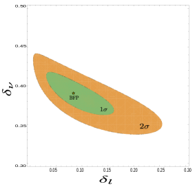
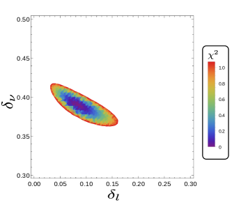
Figure 1: For normal hierarchy. In the left graph, we show the allowed region of the parameters $\delta_{l}$ and $\delta_{\nu}$.

From expressions in Eqs. (33), (35) and (36), we can see that in general the $\chi^{2}$ function depends on five free parameters $\chi^{2}=\chi^{2}\left(\Phi_{1},\Phi_{2},\delta_{l},\delta_{\nu},m_{\nu_{3[2]}}\right)$. But with help of the analysis performed in the previous section, the heaviest neutrino mass is not considered like a free parameter because its numerical values are determined from the experimental data. Hence, the $\chi^{2}$ function has only four free parameters.

Parameter	BFP$\pm 1\sigma$	2$\sigma$	$3\sigma$
$\sin^{2}\theta_{12}(10^{-1})$	$3.26\pm 0.16$	$2.92-3.57$	$2.78-3.75$
$\sin^{2}\theta_{23}(10^{-1})$ [NH]	$5.67_{-1.24}^{+0.32}$	$4.14-6.23$	$3.93-6.43$
$\sin^{2}\theta_{23}(10^{-1})$ [IH]	$5.73_{-0.39}^{+0.25}$	$4.35-6.21$	$4.03-6.40$
$\sin^{2}(\theta_{13})(10^{-2})$ [NH]	$2.26\pm 0.12$	$2.02-5.20$	$1.90-2.60$
$\sin^{2}(\theta_{13})(10^{-2})$ [IH]	$2.29\pm 0.12$	$2.05-2.52$	$1.93-2.65$

Table 2: Experimental results of neutrino mixing angles in the ranges $1\sigma,\,2\sigma$ and $3\sigma$ Forero, Tortola, and Valle (2014).

Now to perform the likelihood test $\chi^{2}$, we consider that the neutrino masses, given in the Table 1, run into the range of $2\sigma$. The values for lepton masses in MeV’s are Olive et al. (2014)

$$\begin{array}[]{l}m_{e}=0.5109998928\pm 0.000000011,\;m_{\mu}=105.6583715\pm 0.0000035,\;\textrm{and}\;m_{\tau}=1776.82\pm 0.16.\end{array}$$ (39)

Then, as result of the minimizing procedure of the $\chi^{2}$ function, for normal hierarchy in neutrino masses we obtain that the values of free parameters in the best fit point (BFP) are the following:

$$\begin{array}[]{ll}\Phi_{1}=-6.789\times 10^{-1}\,\textrm{rad},&\Phi_{2}=2.815\,\textrm{rad},\\ \delta_{l}=8.355\times 10^{-2},&\delta_{\nu}=3.90\times 10^{-1},\\ m_{\nu_{3}}=5.00\times 10^{-2}\,\textrm{eV},&\chi_{\min}^{2}=1.643\times 10^{-9}.\end{array}$$ (40)

As mentioned above the $\chi^{2}$ function depends on four free parameters and three physical observables. Therefore, this function has minus one degrees of freedom, whereby we only can obtain the BFP. However, from Eq. (40) we know the numerical values for the free parameters in the BFP. So, a new analysis is performance fixing the CP violation phase, since this is the parameter less known from the experimental point of view. But, nowadays there are several experiments focussed on its measurement. Then, for a normal hierarchy in leptonic mass spectrum, we fix the value of phases $\Phi_{1}$ and $\Phi_{2}$, as well as the heaviest neutrino mass $m_{\nu_{3[2]}}$ to the values given in Eq. (40). So, the $\chi^{2}=\chi^{2}(\delta_{l},\delta_{\nu})$ function implies one degree of freedom. This last choice allows us to obtain the parameter regions at different confidential levels. The results related to these regions are shown in Figure 1.

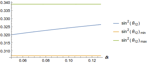
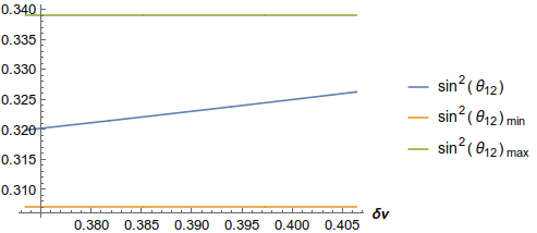
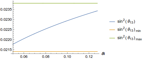
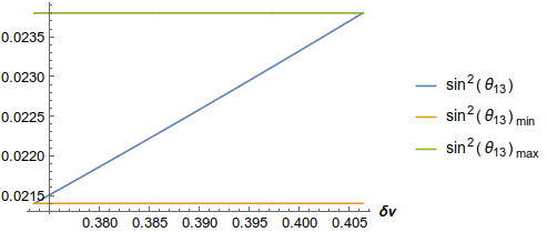
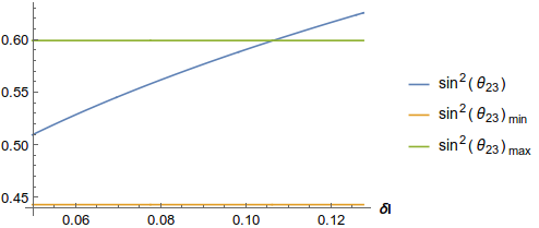
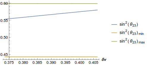
Figure 2: For normal hierarchy. In the left graph, we show the allowed region of the parameters $\delta_{l}$ and $\delta_{\nu}$ to $95\%$ C. L..

IV.3 The lepton mixing angles                                                                                                  

Here, considering the results of the above likelihood test we study the sine of flavour mixing angles given by Eq. (35), as well as the PMNS matrix. In Figure 2, we show the range of theoretical values obtained at $\pm 1\sigma$ as the experimental edge values given in Table 2. One can note that for both $\delta_{l}\&\sin(\theta_{12,13,23})$, and for the $\delta_{\nu}\&\sin(\theta_{12,13,23})$, results are inside the region of $1\sigma$.

As an immediate result of the above likelihood test $\chi^{2}$, the flavour mixing matrix ${\bf V}_{\rm PMNS}$ is numerically computed, at $1\sigma$ C.L.

$${\bf V}_{\rm PMNS}=\begin{pmatrix}8.13\times 10^{-1}\pm 6.06\times 10^{-3}&5.62\times 10^{-1}\pm 6.38\times 10^{-3}&1.50\times 10^{-1}\pm 9.16\times 10^{-3}\\ 2.40\times 10^{-1}\pm 3.91\times 10^{-2}&5.25\times 10^{-1}\pm 4.23\times 10^{-2}&7.44\times 10^{-1}\pm 4.21\times 10^{-2}\\ 4.94\times 10^{-1}\pm 2.68\times 10^{-2}&5.75\times 10^{-1}\pm 3.36\times 10^{-2}&5.60\times 10^{-1}\pm 5.81\times 10^{-2}\end{pmatrix}.$$ (41)

In the above section we have seen that in our theoretical framework, 2HDM+$3\nu$, where the fermion mass matrix have a four-zero texture shape. We can reproduce the values of oscillation parameters in a very good agreement with the last experimental data. The next step in this study shall be to investigate the phenomenological implications of these results for the neutrinoless double beta decay ($0\nu\beta\beta$) and the CP violation in neutrino oscillations in matter.

V  Conclusions                                                                                                                      

In the theoretical framework of Two Higgs Doublet Model type III plus massive neutrinos (2HDM-III+$3\nu$), we shown that can be done we outlined a unified treatment for the fermion mass matrices in the theory. The active neutrinos are considered as Majorana particles and their masses are computed through the type-I seesaw mechanism, where the right-handed neutrinos are introduced in the model as a singlet under the action of the gauge group of the Standard Model. In such a treatment, the mass matrices of Dirac and right-handed neutrinos are represented with a four-zero texture ansatz, which implies that the mass matrix of left-handed neutrinos have also this shape with four-zero texture. In fact, all Dirac fermion mass matrices are represented with the same generic Hermitian matrix with four-zero texture and a normal hierarchy in the mass spectrum. Theoretical expressions were derived for the elements of ${\mathbf{V}}_{\rm PMNS}$ matrix in function of lepton masses, two phases $\Phi_{1}$ and $\Phi_{2}$ associated with the CP violation, and two parameters $\delta_{\nu}$ and $\delta_{\nu}$ which are related with the Yukawa matrices of 2HDM-III. From the theoretical relations of the differences of the squared neutrino masses, and the experimental results reported by the Planck Collaboration and neutrino oscillation experiments, we obtain the allowed values for the neutrino masses. The parameter space exploration is done by means of likelihood test $\chi^{2}$; this allowed us to find the allowed regions of the parameters $\delta_{\nu}$ and $\delta_{l}$ at 70% and 95% C.L. for a normal hierarchy, as well as, the best fit point (BFP), and the mixing matrix ${\mathbf{V}}_{\rm PMNS}$ at 70% C.L. Finally, it is observed that the mixing angle as function of $\delta_{\nu}$ and $\delta_{l}$ are in very good agreement with experimental data.

VI Acknowledgments                                                                                                                

This work has been partially supported by CONACYT-SNI (Mexico). ERJ acknowledges the financial support received from PROFOCIE (Mexico). F.G.C. acknowledges the financial support received from Mexican grants CONACYT 236394, 132059, and PAPIIT IN111115.

References

- Capozzi et al. (2016) Capozzi, F., Lisi, E., Marrone, A., Montanino, D. and Palazzo, A.. “ Neutrino masses and mixings: Status of known and unknown parameters”, (2016) arXiv:1601.07777 [hep-ph] .
- Gando et al. (2011) Gando, A., et al. (KamLAND), “ Constraints on from A Three-Flavor Oscillation Analysis of Reactor Antineutrinos at KamLAND ”, Phys. Rev. D83, p. 052002 (2011), arXiv:1009.4771 [hep-ex] .
- Gando et al. (2013) Gando, A., et al. (KamLAND), “ Reactor On-Off Antineutrino Measurement with KamLAND ”, Phys. Rev. D88, p. 033001 (2013), arXiv:1303.4667 [hep-ex] .
- Seo (2015) Seo, S.-H., (RENO), Proceedings, 26th International Conference on Neutrino Physics and Astrophysics (Neutrino 2014), AIP Conf. Proc. 1666, p. 080002 (2015), arXiv:1410.7987 [hep-ex] .
- Choi et al. (2015) Choi, J. H., et al. (RENO), “ Observation of Energy and Baseline Dependent Reactor Antineutrino Disappearance in the RENO Experiment ”, (2015), arXiv:1511.05849 [hep-ex] .
- Abe et al. (2014) Abe, Y., et al. (Double Chooz), “ Improved measurements of the neutrino mixing angle with the Double Chooz detector ”, JHEP 10, p. 086 (2014), [Erratum: JHEP02,074(2015)], arXiv:1406.7763 [hep-ex] .
- An et al. (2015) An, F. P., et al. (Daya Bay), “ Measurement of the Reactor Antineutrino Flux and Spectrum at Daya Bay ”, Phys. Rev. Lett. 116, p. 061801 (2015), arXiv:1508.04233 [hep-ex] .
- Félix-Beltrán et al. (2015) Félix-Beltrán, O., González-Canales, F., Hernández-Sánchez, J., Moretti, S., Noriega-Papaqui, R., and Rosado, A., “Analysis of the quark sector in the 2HDM with a four-zero Yukawa texture using the most recent data on the CKM matrix ”, Phys. Lett. B742, 347–352 (2015), arXiv:1311.5210 [hep-ph] .
- Atwood, Reina, and Soni (1997) Atwood, D., Reina, L., and Soni, A., “ Phenomenology of two Higgs doublet models with flavor changing neutral currents ”, Phys. Rev. D55, 3156–3176 (1997), arXiv:hep-ph/9609279 [hep-ph] .
- Krawczyk and Sokolowska (2007) Krawczyk, M., and Sokolowska, D., 2007 International Linear Collider Workshop (LCWS07 and ILC07) Hamburg, Germany, May 30-June 3, 2007, eConf C0705302, p. HIG09 (2007), [141(2007)], arXiv:0711.4900 [hep-ph] .
- Krawczyk (2006) Krawczyk, M., Proceedings, 2005 Europhysics Conference on High Energy Physics (EPS-HEP 2005), PoS HEP2005, p. 335 (2006), arXiv:hep-ph/0512371 [hep-ph] .
- Deppisch (2013) Deppisch, F. F., “ Lepton Flavour Violation and Flavour Symmetries ”, Fortsch. Phys. 61, 622–644 (2013), arXiv:1206.5212 [hep-ph] .
- Dorsner and Barr (2002) Dorsner, I., and Barr S. M., “ Flavor exchange effects in models with Abelian flavor symmetry ”, Phys. Rev. D65, p. 095004 (2002), arXiv:hep-ph/0201207 [hep-ph] .
- Fritzsch and zhong Xing (2000) Fritzsch, H., and Zhong Xing, Z., “ Mass and flavor mixing schemes of quarks and leptons ”, Prog. Part. Nucl. Phys. 45, 1–81 (2000), arXiv:hep-ph/9912358 [hep-ph] .
- Schechter and Valle (1980) Schechter, J., and Valle, J. W. F., “ Neutrino Masses in Theories ”, Phys.Rev. D22, p. 2227 (1980) .
- Rodejohann and Valle (2011) Rodejohann, W., and Valle, J. W. F., “Symmetrical Parametrizations of the Lepton Mixing Matrix”, Phys. Rev. D84, p. 073011 (2011), arXiv:1108.3484 [hep-ph] .
- Olive et al. (2014) Olive, K. A., et al. (Particle Data Group), Chin. Phys. C38, p. 090001 (2014) .
- Ade et al. (2015) Ade, P. A. R., et al. (Planck), “Planck 2015 results. XIII. Cosmological parameters”, (2015), arXiv:1502.01589 [astro-ph.CO] .
- Forero, Tortola, and Valle (2014) Forero, D., Tortola, M., and Valle, J., “Neutrino oscillations refitted”, Phys.Rev. D90, p. 093006 (2014), arXiv:1405.7540 [hep-ph] .