Sampling Method for Fast Training of Support Vector Data Description

Abstract

Support Vector Data Description (SVDD) is a popular outlier detection technique which constructs a flexible description of the input data. SVDD computation time is high for large training datasets which limits its use in big-data process-monitoring applications. We propose a new iterative sampling-based method for SVDD training. The method incrementally learns the training data description at each iteration by computing SVDD on an independent random sample selected with replacement from the training data set. The experimental results indicate that the proposed method is extremely fast and provides good data description.

I Introduction

Support Vector Data Description (SVDD) is a machine learning technique used for single class classification and outlier detection. SVDD technique is similar to Support Vector Machines and was first introduced by Tax and Duin [12]. It can be used to build a flexible boundary around single class data. Data boundary is characterized by observations designated as support vectors. SVDD is used in domains where majority of data belongs to a single class. Several researchers have proposed use of SVDD for multivariate process control [11]. Other applications of SVDD involve machine condition monitoring [13, 14] and image classification [10].

I-A Mathematical Formulation of SVDD

Normal Data Description

The SVDD model for normal data description builds a minimum radius hypersphere around the data.

Primal Form

Objective Function:

$$\min R^{2}+C\sum_{i=1}^{n}\xi_{i},$$ (1)

subject to:

$$\|x_{i}-a\|^{2}\leq R^{2}+\xi_{i},\forall i=1,\dots,n,$$ (2)

$$\xi_{i}\geq 0,\forall i=1,...n.$$ (3)

where:
$x_{i}\in{\mathbb{R}}^{m},i=1,\dots,n$ represents the training data,
$R:$ radius, represents the decision variable,
$\xi_{i}:$ is the slack for each variable,
$a$: is the center, a decision variable,
$C=\frac{1}{nf}:$ is the penalty constant that controls the trade-off between the volume and the errors, and,
$f:$ is the expected outlier fraction.

Dual Form

The dual formulation is obtained using the Lagrange multipliers.
Objective Function:

$$\max\ \sum_{i=1}^{n}\alpha_{i}(x_{i}.x_{i})-\sum_{i,j}\alpha_{i}\alpha_{j}(x_{i}.x_{j}),$$ (4)

subject to:

$$\sum_{i=1}^{n}\alpha_{i}=1,$$ (5)

$$0\leq\alpha_{i}\leq C,\forall i=1,\dots,n.$$ (6)

where:
$\alpha_{i}\in\mathbb{R}$: are the Lagrange constants,
$C=\frac{1}{nf}:$ is the penalty constant.

Duality Information

Depending upon the position of the observation, the following results hold: Center Position:

$$\sum_{i=1}^{n}\alpha_{i}x_{i}=a.$$ (7)

Inside Position:

$$\left\|x_{i}-a\right\|<R\rightarrow\alpha_{i}=0.$$ (8)

Boundary Position:

$$\left\|x_{i}-a\right\|=R\rightarrow 0<\alpha_{i}<C.$$ (9)

Outside Position:

$$\left\|x_{i}-a\right\|>R\rightarrow\alpha_{i}=C.$$ (10)

The radius of the hypersphere is calculated as follows:

$$R^{2}=(x_{k}.x_{k})-2\sum_{i}\alpha_{i}(x_{i}.x_{k})+\sum_{i,j}\alpha_{i}\alpha_{j}(x_{i}.x_{j}).$$ (11)

using any $x_{k}\in SV_{<C}$ , where $SV_{<C}$ is the set of support vectors that have $\alpha_{k}<C$.

Scoring

For each observation $z$ in the scoring data set, the distance $\textrm{dist}^{2}(z)$ is calculated as:

$$dist^{2}(z)=(z.z)-2\sum_{i}\alpha_{i}(x_{i}.z)+\sum_{i,j}\alpha_{i}\alpha_{j}(x_{i}.x_{j})$$ (12)

and observations with $dist^{2}(z)>R^{2}$ are designated as outliers.

The spherical data boundary can include a significant amount of space with a very sparse distribution of training observations which leads to a large number of falses positives. The use of kernel functions leads to better compact representation of the training data.

Flexible Data Description

The Support Vector Data Description is made flexible by replacing the inner product $(x_{i}.x_{j})$ in equation (11) with a suitable kernel function $K(x_{i},x_{j})$. The Gaussian kernel function used in this paper is defined as:

$$K(x_{i},x_{j})=\exp\dfrac{-\|x_{i}-x_{j}\|^{2}}{2s^{2}}$$ (13)

where $s$: Gaussian bandwidth parameter.

The modified mathematical formulation of SVDD with kernel function is:

Objective function:

$$\max\ \sum_{i=1}^{n}\alpha_{i}K(x_{i},x_{i})-\sum_{i,j}\alpha_{i}\alpha_{j}K(x_{i},x_{j}),$$ (14)

Subject to:

$$\sum_{i=1}^{n}\alpha_{i}=1,$$ (15)

$$0\leq\alpha_{i}\leq C=\frac{1}{nf},\forall i=1,\dots,n.$$ (16)

Conditions similar to (7) to (10) continue to hold even when the kernel function is used.
The threshold $R^{2}$ is calculated as :

$$R^{2}=K(x_{k},x_{k})-2\sum_{i}\alpha_{i}K(x_{i},x_{k})+\sum_{i,j}\alpha_{i}\alpha_{j}K(x_{i},x_{j})$$ (17)

using any $x_{k}\in SV_{<C}$ , where $SV_{<C}$ is the set of support vectors that have $\alpha_{k}<C$.

Scoring

For each observation $z$ in the scoring dataset, the distance $dist^{2}(z)$ is calculated as:

$$dist^{2}(z)=K(z,z)-2\sum_{i}\alpha_{i}K(x_{i},z)+\sum_{i,j}\alpha_{i}\alpha_{j}K(x_{i},x_{j}),$$ (18)

and the observations with $dist^{2}(z)>R^{2}$ are designated as outliers.

II Need for a Sampling-based Approach

As outlined in Section I-A, SVDD of a data set is obtained by solving a quadratic programming problem. The time required to solve the quadratic programming problem is directly related to the number of observations in the training data set. The actual time complexity depends upon the implementation of the underlying Quadratic Programming solver. We used LIBSVM to evaluate SVDD training time as a function of the training data set size. We have used C++ code that uses LIBSVM  [2] implementation of SVDD the examples in this paper, we have also provided a Python implmentation which uses Scikit-learn [8] at [1]. Figure 1 shows processing time as a function of training data set size for the two donut data set (see Figure 3c for a scatterplot of the two donut data). In Figure 1 the x-axis indicates the training data set size and the y-axis indicates processing time in minutes. As indicated in Figure 1, the SVDD training time is low for small or moderately sized training data but gets prohibitively high for large datasets.

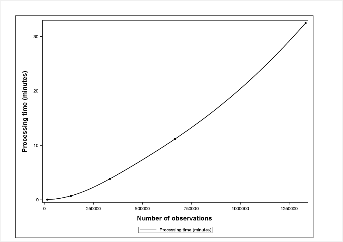
Figure 1: SVDD Training Time: Two Donut data

There are applications of SVDD in areas such as process control and equipment health monitoring where size of training data set can be very large, consisting of few million observations. The training data set consists of sensors readings measuring multiple key health or process parameters at a very high frequency. For example, a typical airplane currently has $\approx$7,000 sensors measuring critical health parameters and creates 2.5 terabytes of data per day. By 2020, this number is expected to triple or quadruple to over 7.5 terabytes [4]. In such applications, multiple SVDD training models are developed, each representing separate operating mode of the equipment or process settings. The success of SVDD in these applications require algorithms which can train using huge amounts of training data in an efficient manner.

To improve performance of SVDD training on large data sets, we propose a new sampling based method. Instead of using all observations from the training data set, the algorithm computes the training data SVDD by iteratively computing SVDD on independent random samples obtained from the training data set and combining them. The method works well even when the random samples have few observations. We also provide a criteria for detecting convergence. At convergence the our method provides a data description that compares favorably with result obtained by using all the training data set observations.

The rest of this document is organized as follows: Section III provides details of the proposed sampling-based iterative method. Results of training with the proposed method are provided in section IV; the analysis of high dimensional data is provided in section V; the results of a simulation study on random polygons is provided in section Section VI and we provide our conclusions in section VII.

Note: In the remainder of this paper, we refer to the training method using all observations in one iteration as the full SVDD method.

III Sampling-based Method

The Decomposition and Combination method of Luo et.al.[7] and K-means Clustering Method of Kim et.al.[5], both use sampling for fast SVDD training, but are computationally expensive. The first method by Lou et.al. uses an iterative approach and requires one scoring action on the entire training data set per iteration. The second method by Kim et.al. is a classic divide and conquer algorithm. It uses each observation from the training data set to arrive at the final solution.

In this section we describe our sampling-based method for fast SVDD training. The method iteratively samples from the training data set with the objective of updating a set of support vectors called as the master set of support vectors ($SV^{*}$). During each iteration, the method updates $SV^{*}$ and corresponding threshold $R^{2}$ value and center $a$. As the threshold value $R^{2}$ increases, the volume enclosed by the $SV^{*}$ increases. The method stops iterating and provides a solution when the threshold value $R^{2}$ and the center $a$ converge. At convergence, the members of the master set of support vectors $SV^{*}$, characterize the description of the training data set. For all test cases, our method provided a good approximation to the solution that can be obtained by using all observations in the training data set.

Our method addresses drawbacks of existing sampling based methods proposed by Luo et.al.[7] and Kim et.al.[5]. In each iteration, our method learns using very a small sample from the training data set during each step and typically uses a very small subset of the training data set. The method does not require any scoring actions while it trains.

The sampling method works well for different sample sizes for the random draws in the iterations. It also provides a better alternative to training SVDD on one large random sample from the training data set, since establishing a right size, especially with high dimensional data, is a challenge.

The important steps in this algorithm are outlined below:
Step 1: The algorithm is initialized by selecting a random sample $S_{0}$ of size $n$ from the training data set of $M$ observations ($n\ll M$). SVDD of $S_{0}$ is computed to obtain the corresponding set of support vectors $SV_{0}$. The set $SV_{0}$ initializes the master set of support vectors $SV^{*}$. The iteration number $i$ is set to 1.
Step 2: During this step, the algorithm updates the master set of support vectors, $SV^{*}$ until the convergence criteria is satisfied. In each iteration $i$, following steps are executed: Step 2.1: A random sample $S_{i}$ of size $n$ is selected and its SVDD is computed. The corresponding support vectors are designated as $SV_{i}$.
Step 2.2: A union of $SV_{i}$ with the current master set of support vectors, $SV^{*}$ is taken to obtain a set $S_{i}^{{}^{\prime}}$ ($S_{i}^{{}^{\prime}}=SV_{i}\bigcup SV^{*}$).
Step 2.3: SVDD of $S_{i}^{{}^{\prime}}$ is computed to obtain corresponding support vectors $SV_{i}^{{}^{\prime}}$, threshold value $R_{i}^{2}$ and “center” $a_{i}$ (which we define as $\sum_{i}\alpha_{i}x_{i}$ even when a Kernel is used). The set $SV_{i}^{{}^{\prime}}$, is designated as the new master set of support vectors $SV^{*}$. Convergence Criteria: At the end of each iteration $i$, the following conditions are checked to determine convergence.

1. $i$ = $maxiter$, where $maxiter$ is the maximum number of iteration; or
   

2. $\|a_{i}-a_{i-1}\|\leq\epsilon_{1}\|a_{i-1}\|$, and $\left\|R_{i}^{2}-R_{i-1}^{2}\right\|\leq\epsilon_{2}R_{i-1}^{2}$ where $\epsilon_{1},\epsilon_{2}$ are appropriately chosen tolerance parameters.

If the maximum number of iterations is reached or the second condition satisfied for $t$ consecutive iterations, convergence is declared. In many cases checking the convergence of just $R_{i}^{2}$ suffices.

The pseudo-code for this method is provided in algorithm 1. The pseudo-code uses following notations:

1. $S_{i}\leftarrow SAMPLE(T,n)$ denotes the data set $S_{i}$ obtained by selecting random sample of size $n$ from data set $T$.

2. $\delta S_{i}$ denotes SVDD computation on data set $S_{i}$.

3. $\langle SV_{i},R_{i}^{2},a_{i}\rangle\leftarrow\delta S_{i}$ denotes the set of support vectors $SV_{i}$, threshold value $R_{i}^{2}$ and center $a_{i}$ obtained by performing SVDD computations on data set $S_{i}$.

Algorithm 1 Sampling-based iterative method

1:$T$ (training data set) , $n$ (sample size), convergence criteria, $s$ (Gaussian bandwidth parameter), $f$ (fraction of outliers) and $t$ (required number of consecutive observations satisfying convergence criteria ).

2:$S_{0}\leftarrow SAMPLE(T,n)$

3:$\langle SV_{0},R_{0}^{2},a_{0}\rangle\leftarrow\delta S_{0}$

4:$SV^{*}\leftarrow SV_{0}$

5:$i=1$

6:while (Convergence criteria not satisfied for $t$ consecutive obs) do

7:     $S_{i}\leftarrow SAMPLE(T,n)$

8:     $\langle SV_{i},R_{i}^{2},a_{i}\rangle\leftarrow\delta S_{i}$

9:     $S_{i}^{{}^{\prime}}\leftarrow SV_{i}\bigcup SV^{*}$.

10:     $\langle SV_{i}^{{}^{\prime}},R_{i}^{2^{\prime}},a_{i}^{{}^{\prime}}\rangle\leftarrow\delta S_{i}^{{}^{\prime}}$

11:     Test for convergence

12:     $SV^{*}\leftarrow SV_{i}^{{}^{\prime}}$

13:     $i=i+1$

14:end while

15:return $SV^{*}$

As outlined in steps 1 and 2, the algorithm obtains the final training data description by incrementally updating the master set of support vectors $SV^{*}$. During each iteration, the algorithm first selects a small random sample $S_{i}$, computes its SVDD and obtains corresponding set of support vectors, $SV_{i}$. The support vectors of set $SV_{i}$ are included in the master set of support vectors $SV^{*}$ to obtain $S_{i}^{{}^{\prime}}$ ($S_{i}^{{}^{\prime}}=SV_{i}\bigcup SV^{*}$). The set $S_{i}^{{}^{\prime}}$ thus represents an incremental expansion of the current master set of support vectors $SV^{*}$. Some members of $SV_{i}$ can be potentially “inside” the data boundary characterized by $SV^{*}$ the next SVDD computation on $S_{i}^{{}^{\prime}}$ eliminates such “inside” points. During initial iterations as $SV^{*}$ gets updated, its threshold value $R_{i}^{2^{\prime}}$ typically increases and the master set of support vectors expands to describe the entire data set.

Each iteration of our algorithm involves two small SVDD computations and one union operation. The first SVDD computation is fast since it is perfomed on a small sample of training data set. For the remaining two operations, our method exploits the fact that for most data sets support vectors obtained from SVDD are a tiny fraction of the input data set and both the union operation and the second SVDD computation are fast. So our method consists of three fast operations per iteration. For most large datasets we have experimented on the time to convergence is fast and we achieve a reasonable approximation to full SVDD in a fraction to time needed compute SVDD with the full dataset.

III-1 Distributed Implementation

For extremely large training datasets, efficiency gains using distributed implementation are possible. Figure 2 describes SVDD solution using the sampling method outlined in section III utilizing a distributed architecture. The training data set with $M$ observations is first distributed over $p$ worker nodes. Each worker node computes SVDD of its $\dfrac{M}{p}$ observations using the sampling method to obtain its own master set of support vectors $SV_{i}^{*}$. Once SVDD computations are completed, each worker node promotes its own master set of support vectors $SV_{i}^{*}$, to the controller node. The controller node takes a union of all worker node master sets of support vectors, $SV_{i}^{*}$ to create data set $S^{{}^{\prime}}$. Finally, solution is obtained by performing SVDD computation on $S^{{}^{\prime}}$. The corresponding set of support vectors $SV^{*}$ are used to approximate the original training data set description.

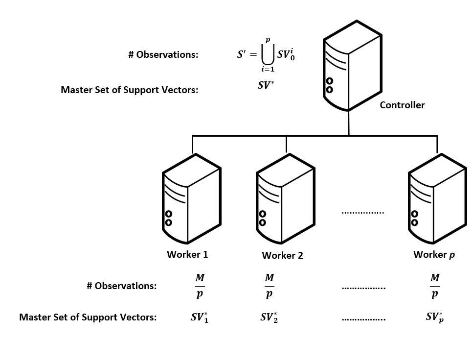
Figure 2: Distributed Implementation

IV Results

To test our method we experimented with three data sets of known geometry which we call the Banana-shaped, Star-shaped, and Two-Donut-shaped data. The figures 3a-3c illustrate these three data sets.

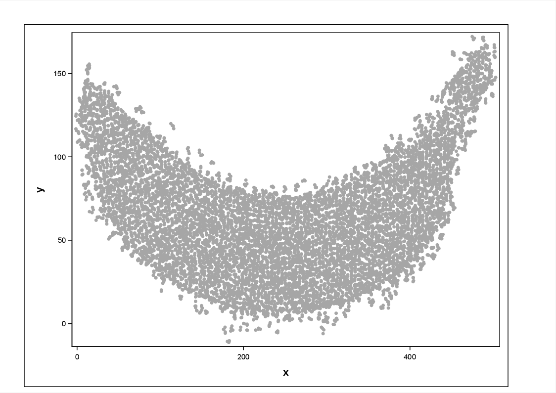
(a) Banana-shaped data

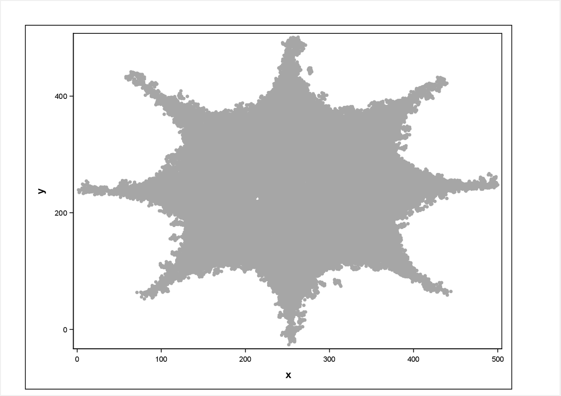
(b) Star-shaped data

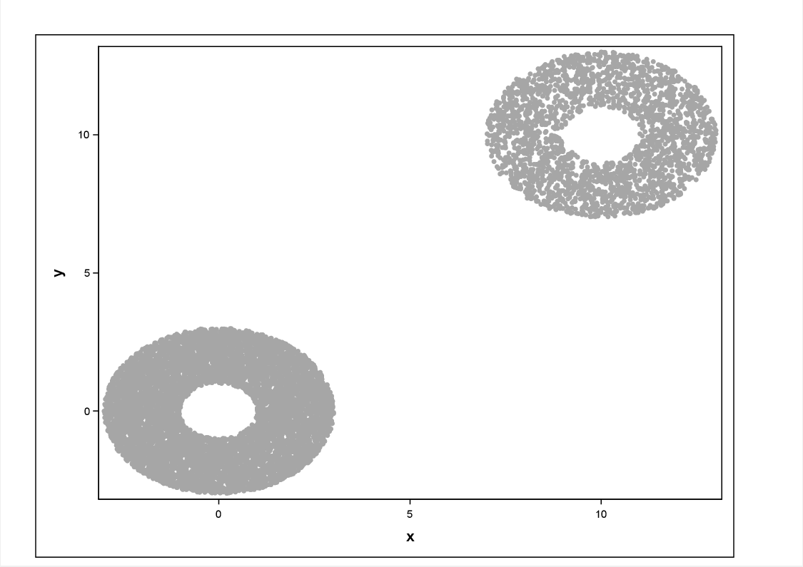
(c) Two-donut-shaped data

Figure 3: Scatter plots

For each data set, we first obtained SVDD using all observations. Table II summarizes the results.
For each data set, we varied the value of the sample size $n$ from 3 to 20 and obtained multiple SVDD using the sampling method. For each sample size value, the total processing time and number of iterations till convergence was noted. Figures 4a to 6 illustrate the results. The vertical reference line indicates the sample size corresponding to the minimum processing time. Table II provides the minimum processing time, corresponding sample size and other details for all three data sets. Figure 7 shows the convergence of threshold $R^{2}$ for the Banana-shaped data trained using sampling method.

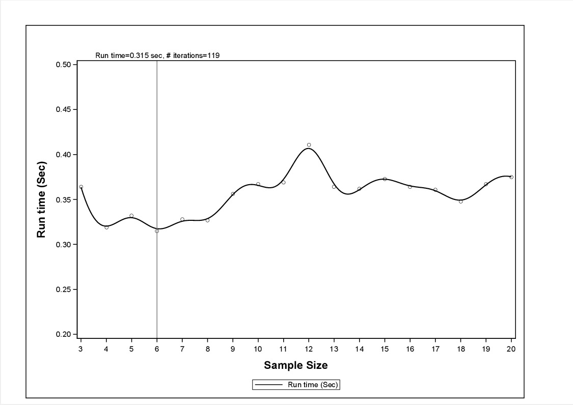
(a) Run time vs. sample size

Figure 4: Banana-shaped data

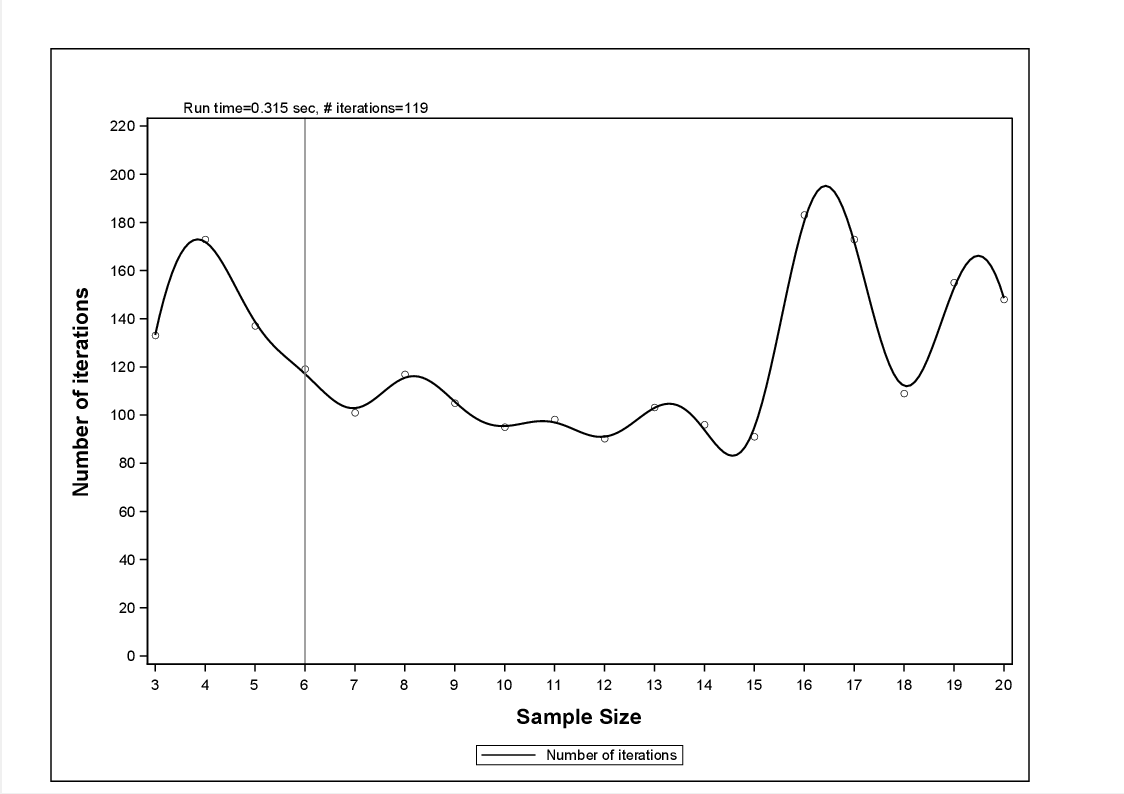
(b) # iterations vs. sample size

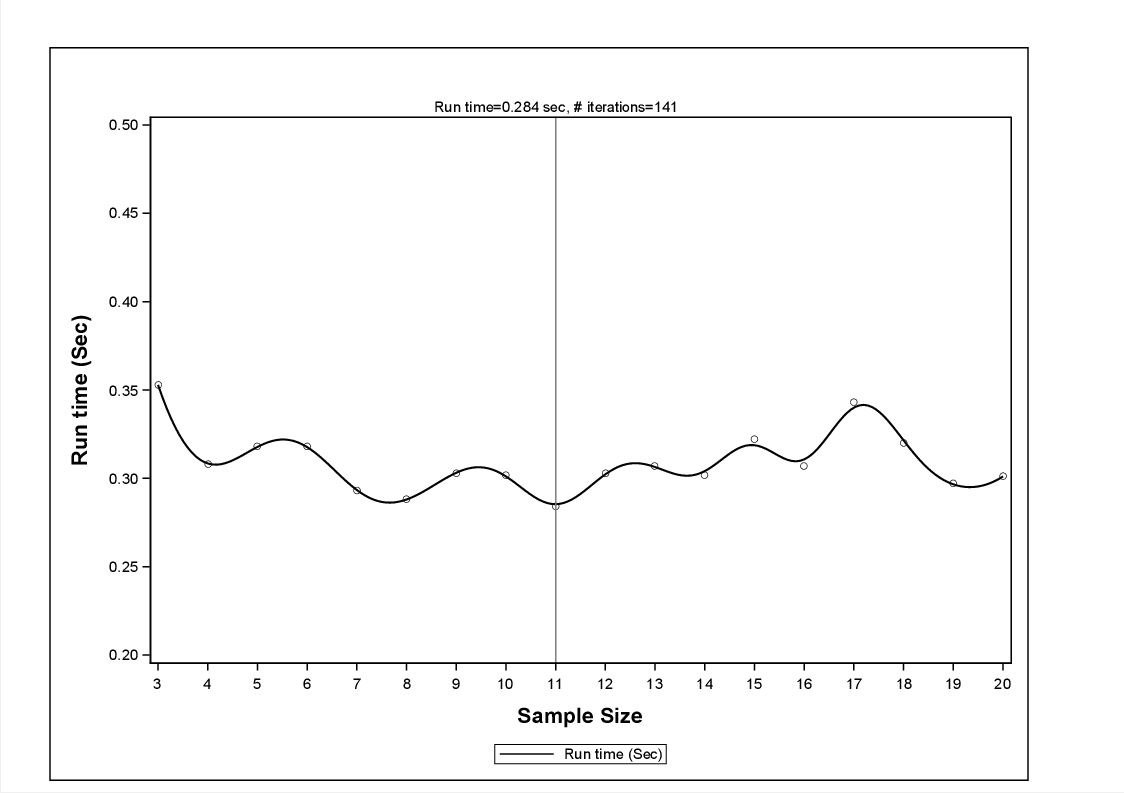
(a) Run time vs. sample size

Figure 5: Star-shaped data

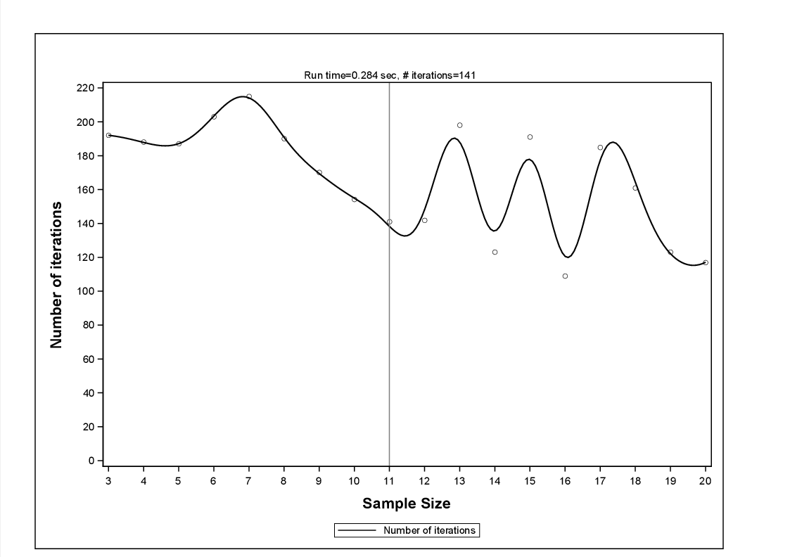
(b) # iterations vs. sample size

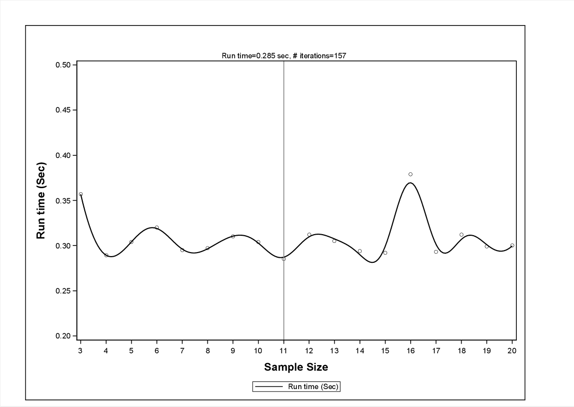
(a) Run time vs. sample size

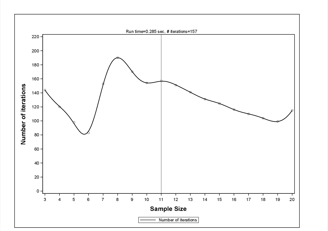
(b) # iterations vs. sample size

Figure 6: Two Donut data

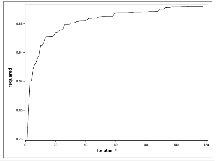
Figure 7: Plot of threshold $R^{2}$ - Banana shaped data (Sample size = 6)

Data	#Obs	$R^{2}$	#SV	Time
Banana	11,016	0.8789	21	1.98 sec
TwoDonut	1,333,334	0.8982	178	32 min
Star	64,000	0.9362	76	11.55 sec

TABLE I: SVDD Training using full SVDD method

Data Iterations $R^{2}$ #SV Time Banana(6) 119 0.872 19 0.32 sec TwoDonut(11) 157 0.897 37 0.29 sec Star(11) 141 0.932 44 0.28 sec TABLE II: SVDD Results using Sampling Method (sample size in parenthesis)

Results provided in Table II and Table II indicate that our method provides an order of magnitude performance improvement as compared to training using all observations in a single iteration. The threshold $R^{2}$ values obtained using the sampling-based method are approximately equal to the values that can be obtained by training using all observations in a single iteration. Although the radius values are same, to confirm if the data boundary defined using support vectors is similar, we performed scoring on a $200\times 200$ data grid. Figure 8 provides the scoring results for all data sets. The scoring results for the Banana-shaped and the Two-Donut-shaped are very similar for both the method, the scoring results for the Star-shaped shaped data for the two methods are also similar except for a region near the center.

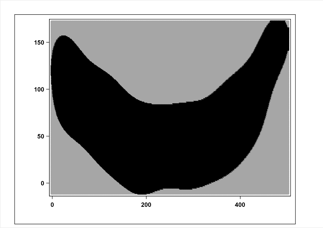
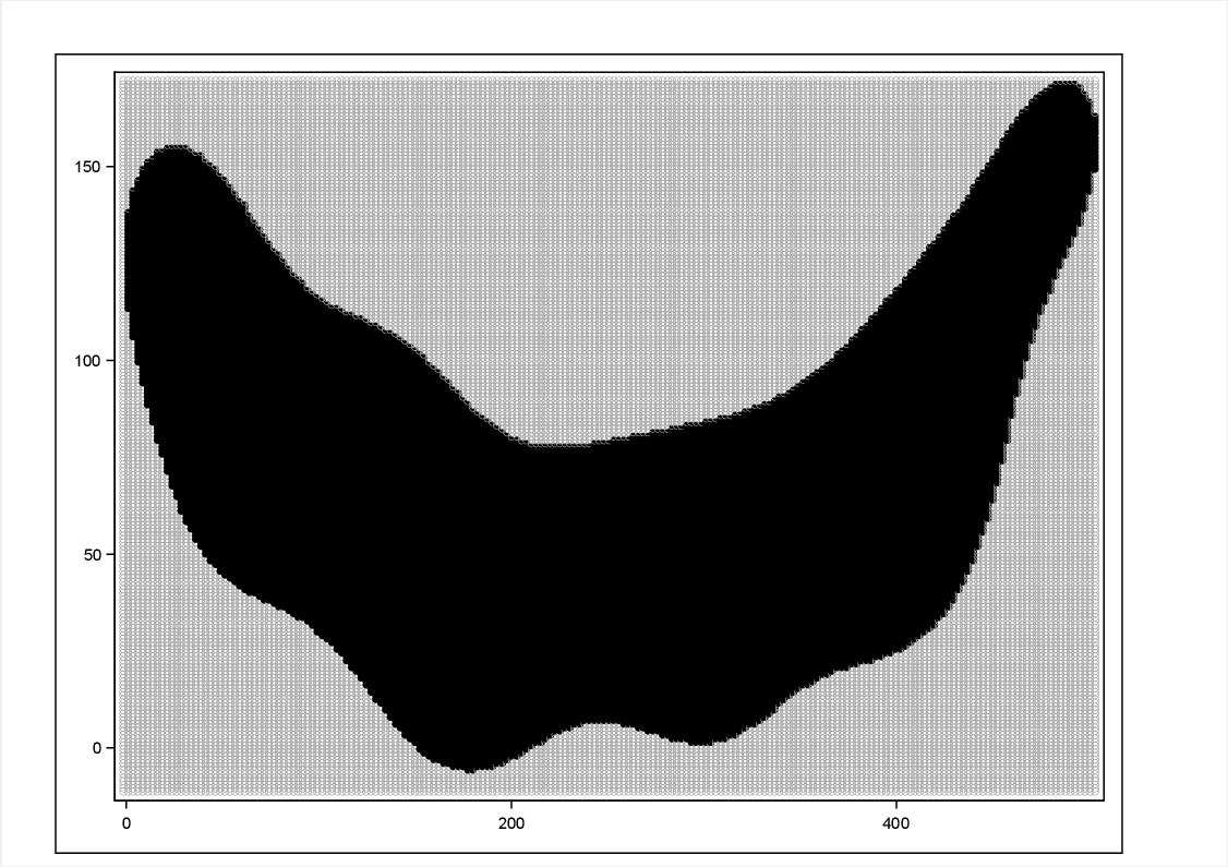
(a)	(b)
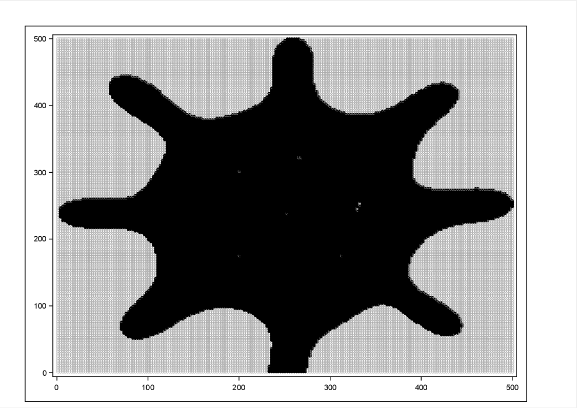
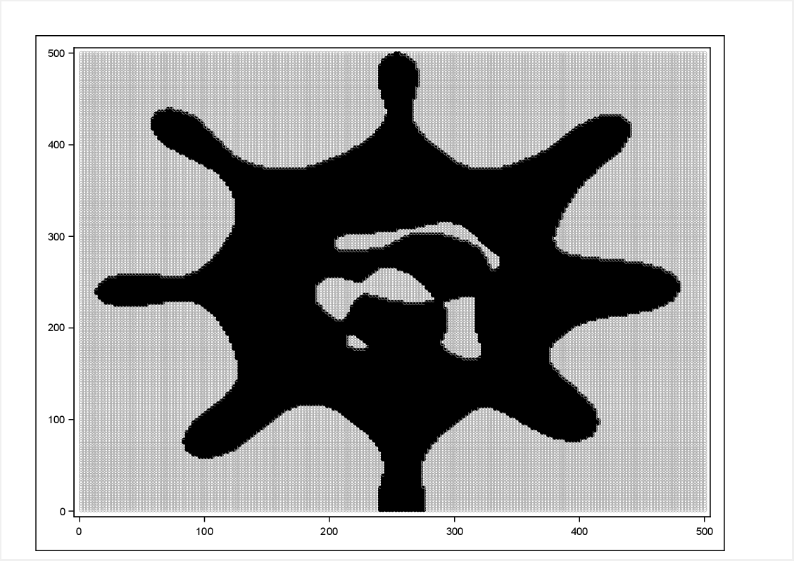
(a)	(b)
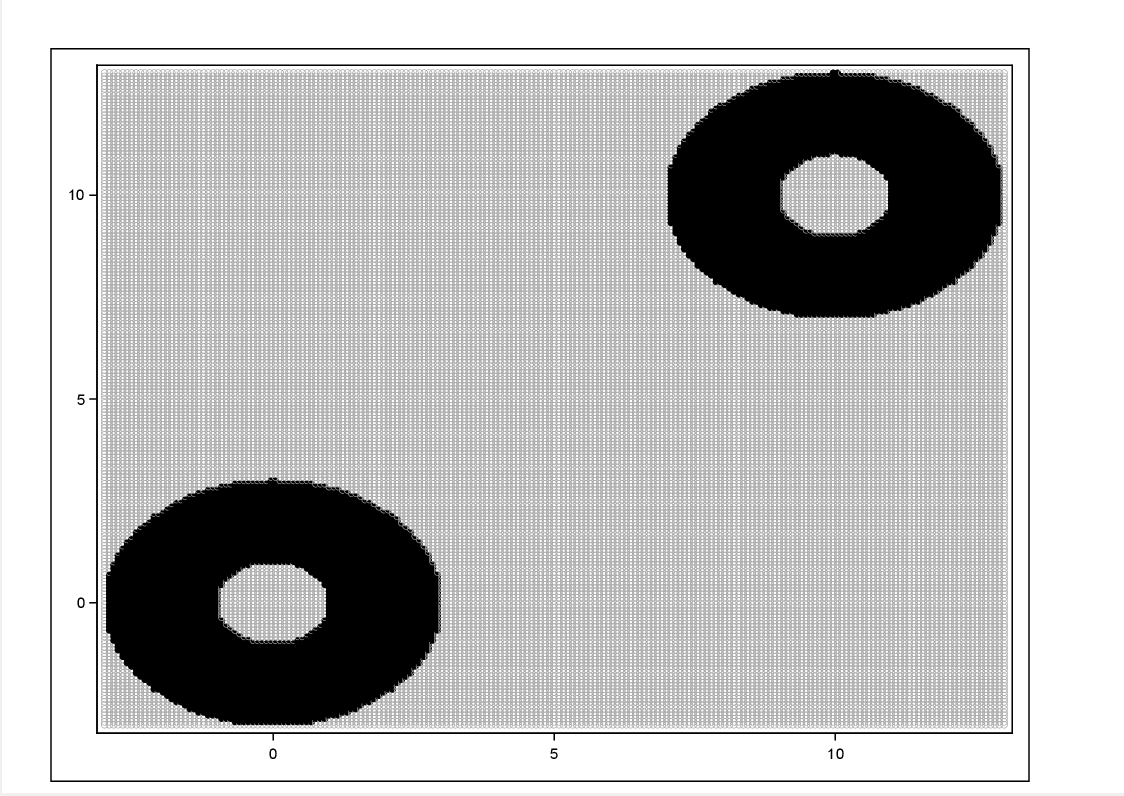
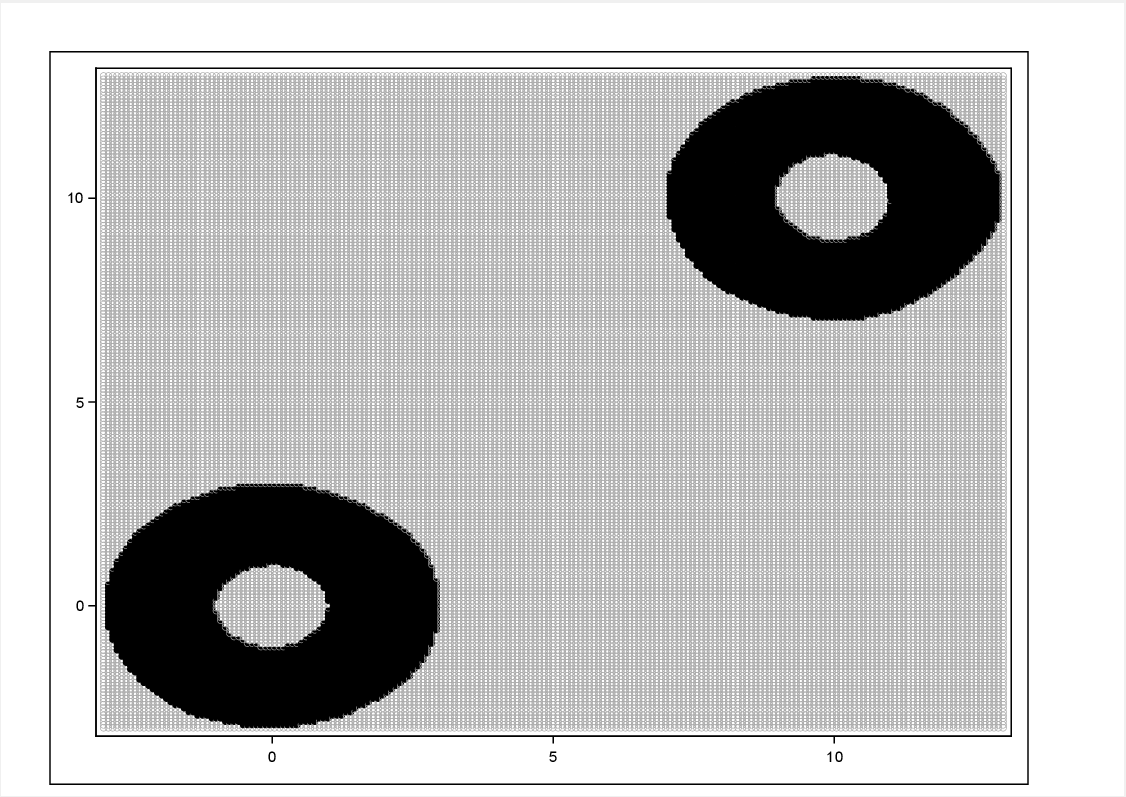
(a)	(b)
Full SVDD Method	Sampling method

Figure 8: Scoring results. Above figures show results of scoring on a 200x200 data grid. Light gray color indicates outside points and black color indicates inside points. Figure (a) used full SVDD method for training. Figure (b) used sampling method for training.

V Analysis of High Dimensional Data

Section IV provided comparison of our sampling method with full SVDD method. For two-dimensional data sets the performance of sampling method can be visually judged using the scoring results. We tested the sampling method with high dimensional datasets, where such visual feedback about classification accuracy of sampling method is not available. We compared classification accuracy of the sampling method with the accuracy of training with full SVDD method. We use the $F_{1}$-measure to quantify the classification accuracy [15]. The $F_{1}$-measure is defined as follows:

$$F_{1}=\dfrac{2\times\text{Precision}\times\text{Recall}}{\text{Precision}+\text{Recall}},$$ (19)

where:

$$\text{Precision}=\dfrac{\text{true positives}}{\text{true positives}+\text{false positives}}$$ (20)

$$\text{Recall}=\dfrac{\text{true positives}}{\text{true positives}+\text{false negatives}}.$$ (21)

Thus high precision relates to a low false positive rate, and high recall relates to a low false negative rate. We chose the $F_{1}$-measure because it is a composite measure that takes into account both the Precision and the Recall. Models with higher values of $F_{1}$-measure provide a better fit.

V-A Analysis of Shuttle Data

In this section we provide results of our experiments with Statlog (shuttle) dataset [6]. This is a high dimensional data consists of nine numeric attributes and one class attribute. Out of 58,000 total observations, 80% of the observations belong to class one. We created a training data set of randomly selected 2,000 observations belonging to class one. The remaining 56,000 observations were used to create a scoring data set. SVDD model was first trained using all observations in the training data set. The training results were used to score the observations in the scoring data set to determine if the model could accurately classify an observation as belonging to class one and the accuracy of scoring was measured using the $F_{1}$-measure. We then trained using the sampling-based method, followed by scoring to compute the $F_{1}$-measure again. The sample size for the sampling-based method was set to 10 (number of variables + 1). We measured the performance of the sampling method using the $F_{1}$-measure ratio defined as $F_{\text{Sampling}}/F_{\text{Allobs}}$ where $F_{\text{Sampling}}$ is the $F_{1}$-measure obtained when the value obtained using the sampling method for training, and $F_{\text{Allobs}}$ is the value of $F_{1}$-measure computed when all observations were used for training. A value close to 1 indicate that sampling method is competitive with full SVDD method. We repeated the above steps varying the training data set of size from 3,000 to 40,000 in the increments of 1,000. The corresponding scoring data set size changed from 55,000 to 18,000. Figure 9 provides the plot of $F_{1}$-measure ratio. The plot of $F_{1}$-measure ratio is constant, very close to 1 for all training data set sizes, provides the evidence that our sampling method provides near identical classification accuracy as compared to full SVDD method. Figure 10 provides the plot of the processing time for the sampling method and training using all obsrvations. As the training data set size increased, the processing time for full SVDD method increased almost linearly to a value of about 5 seconds for training data set of 40,000 observations. In comparison, the processing time of the sampling based method was in the range of 0.24 to 0.35 sec. The results prove that the sampling-based method is efficient and it provides near identical results to full SVDD method.

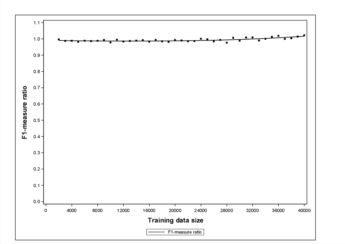
Figure 9: $F_{1}$-measure plot: Shuttle data. Sample size for sampling method=10

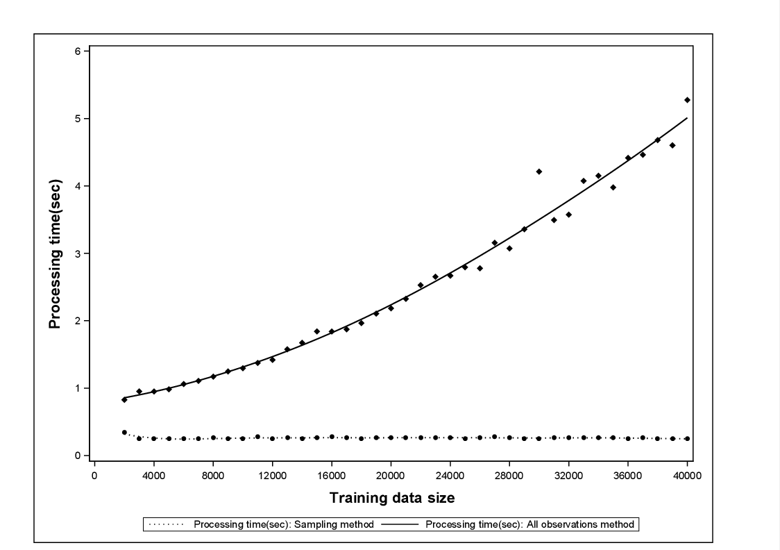
Figure 10: Processing time plot: Shuttle data. Sample size for sampling method=10

V-B Analysis of Tennessee Eastman Data

In this section we provide results of our experiments with high dimensional Tennessee Eastman data. The data was generated using the MATLAB simulation code [9] which provides a model of an industrial chemical process [3]. The data was generated for normal operations of the process and twenty faulty processes. Each observation consists of 41 variables, out of which 22 are measured continuously, on an average, every 6 seconds and remaining 19 sampled at a specified interval either every 0.1 or 0.25 hours. We interpolated the 22 observations which are measured continuously using SAS^® EXPAND procedure. The interpolation increased the observation frequency and generated 20 observations per second. The interpolation ensured that we have adequate data volume to compare performance our sampling method with full SVDD method.

We created a training data set of 5,000 randomly selected observations belonging to the normal operations of the process. From the remaining observations, we created a scoring data of 228,000 observations by randomly selecting 108,000 observations belonging to the normal operations and 120,000 observations belonging to the faulty processes. A SVDD model was first trained using all observations in the training data set. The training results were used to score the observations in the scoring data set to determine if the model could accurately classify an observation as belonging to the normal operations. The accuracy of scoring was measured using the $F_{1}$-measure. We then trained using the sampling method, followed by scoring to compute the $F_{1}$-measure again. The sample size for the sampling based method was set to 42 (number of variables + 1). Similar to the Shuttle data analysis, we measured the performance of the sampling method using the $F_{1}$-measure ratio defined as $F_{\text{Sampling}}/F_{\text{Allobs}}$ where $F_{\text{Sampling}}$ is the $F_{1}$-measure obtained when the value obtained using the sampling method for training, and $F_{\text{Allobs}}$ is the value of $F_{1}$-measure computed when all observations were used for training. A value close to 1 indicate that sampling method is competitive with full SVDD method.

We repeated the above steps varying the training data set of size from 10,000 to 100,000 in the increments of 5,000. The scoring data set was kept unchanged during each iteration. Figure 11 provides the plot of $F_{1}$-measure ratio. The plot of $F_{1}$-measure ratio was constant, very close to 1 for all training data set sizes, provides the evidence that the sampling method provides near identical classification accuracy as compared to full SVDD method. Figure 12 provides the plot of the processing time for the sampling-based method and the all obsrvation method. As the training data set size increased, the processing time for full SVDD method increased almost linearly to a value of about one minute for training data set of 100,000 observations. In comparison, the processing time of the sampling based method was in the range of 0.5 to 2.0 sec. The results prove that the sampling-based method is efficient and it provides and closely approximates the results obtained from full SVDD method.

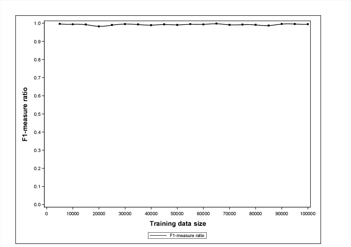
Figure 11: $F_{1}$-measure ratio plot: Tennessee Eastman data. Sample size for sampling method=42

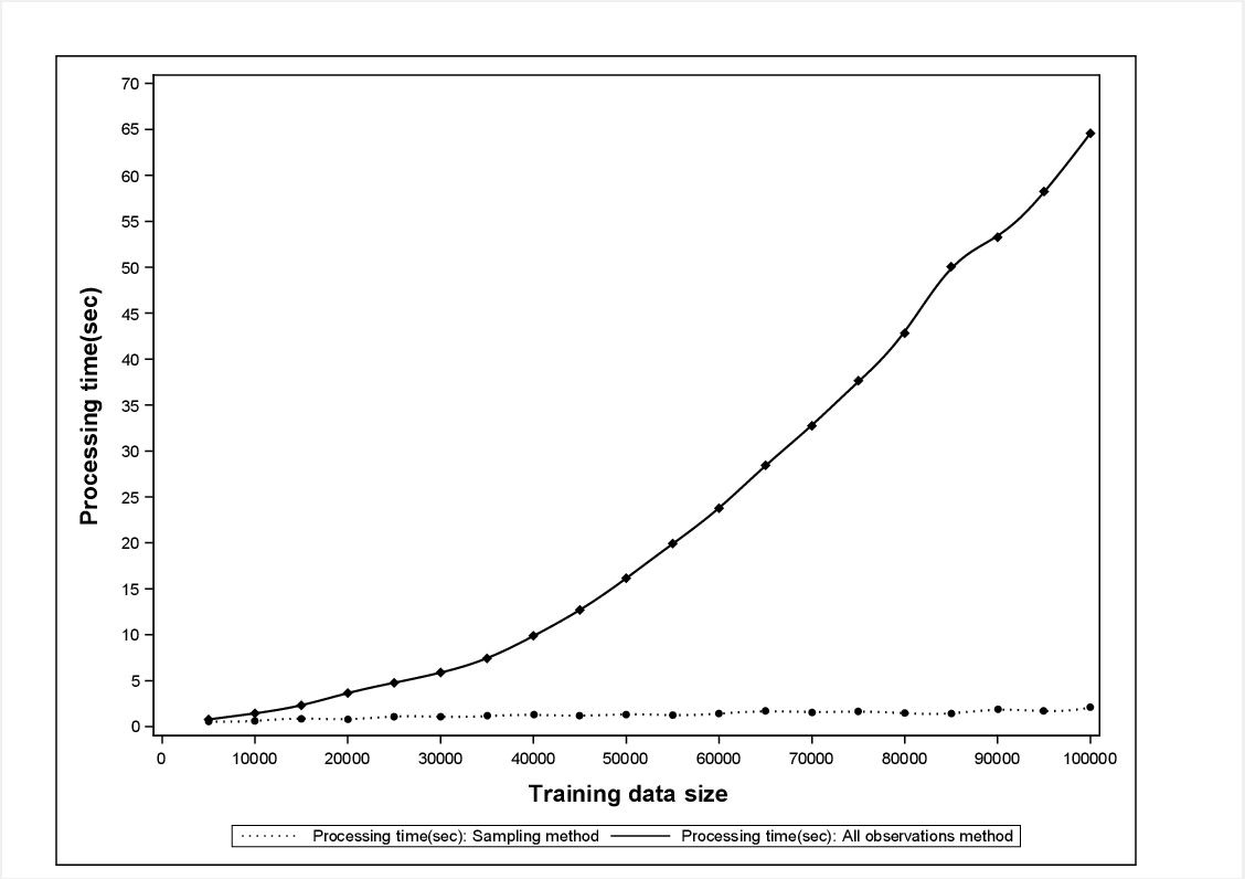
Figure 12: Processing time plot: Tennessee Eastman data. Sample size for sampling method=42

VI Simulation Study

In this section we measure the accuracy of Sampling method when it is applied to randomly generated polygons. Given the number of vertices, $k$,we generate the vertices of a randomly generated polygon in the anticlockwise sense as $r_{1}\exp i\theta_{(1)},\dots,r_{k}\exp i\theta_{(k)}.$ Here $\theta_{(i)}$’s are the order statistics of an i.i.d sample uniformly drawn from $(0,2\pi)$ and $r_{i}$’s are uniformly drawn from an interval $[\text{r}_{\text{min}},\text{r}_{\text{max}}].$ For this simulation we chose $\text{r}_{\text{min}}=3$ and $\text{r}_{\text{max}}=5$ and varied the number of vertices from $5$ to $30$. We generated $20$ random polygons for each vertex size. Figure 13a shows two random polygons. Having determined a polygon we randomly selected $600$ points uniformly from the interior of the polygon to construct a training data set.

To create the scoring data set we the divided the bounding rectangle of each polygon into a $200\times 200$ grid. We labeled each point on this grid as an “inside” or an “outside” point. We then fit SVDD on the training data set and scored the corresponding scoring data set and calculated the $F_{1}$-measure. The process of training and scoring was first performed using the full SVDD method, followed by the sampling method. For sampling method we used sample size of 5. We trained and scored each instance of a polygon 10 times by changing the value of the Gaussian bandwidth parameter, $s$. We used $s$ values from the following set:$s=[1,1.44,1.88,2.33,2.77,3.22,3.66,4.11,4.55,5].$

As in previous examples we used the $F_{!}$ measure ratio to judge the accuracy of the sampling method.

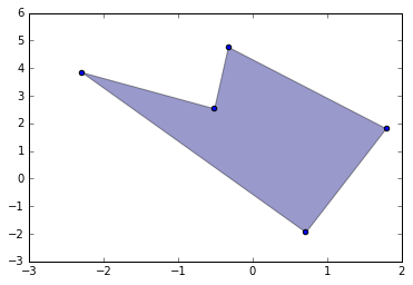
(a) Number of Vertices = 5

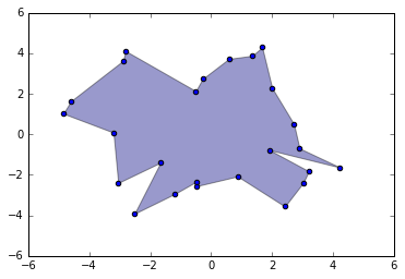
(b) Number of Vertices = 25

Figure 13: Random Polygons

The Box-whisker plots in figures 14 to 15 summarize the simulation study results. The x- axis shows the number of vertices of the ploygon and y-axis shows the $F_{1}$-measure ratio. The bottom and the top of the box shows the first and the third quartile values. The ends of the whiskers represent the minimum and the maximum value of the $F_{1}$-measure ratio. The diamond shape indicates the mean value and the horizontal line in the box indicates the second quartile.

VI-A Comparison of the best fit across $s$

For each instance of a polygon we looked at $s$ value which provides the best fit in terms of the $F_{1}$-ratio for each of the methods. The plot in Figure 14 shows the plot of $F_{1}$ measure ratio computed using the maximum values of $F_{1}$ measures. The plot shows that $F_{1}$-measure ratio is greater than $\approx 0.92$ across all values of number of vertices. The $F_{1}$ measure ratio in the top three quartiles is greater than $\approx$ 0.97 across all values of the number of vertices. Using best possible value of s, the sampling method provides comparable results with full SVDD method.

Figure 14: Box-whisker plot: Number of vertices vs. Ratio of max $F_{1}$ measures

VI-B Results Using Same Value of $s$

We evaluated sampling method against full SVDD method, for the same value of $s$. The plots in Figure 14 illustrate the results for different six different values of $s$. The plot shows that except for one outlier result in Figure 14 (d), $F_{1}$-measure ratio is greater than 0.9 across number of vertices and $s$. In Figures 14 (c) to (f), the top three quartiles of $F_{1}$ measure ratio was consistently greater than $\approx 0.95$. Training using sampling method and full SVDD method, using same $s$ value, provide similar results.

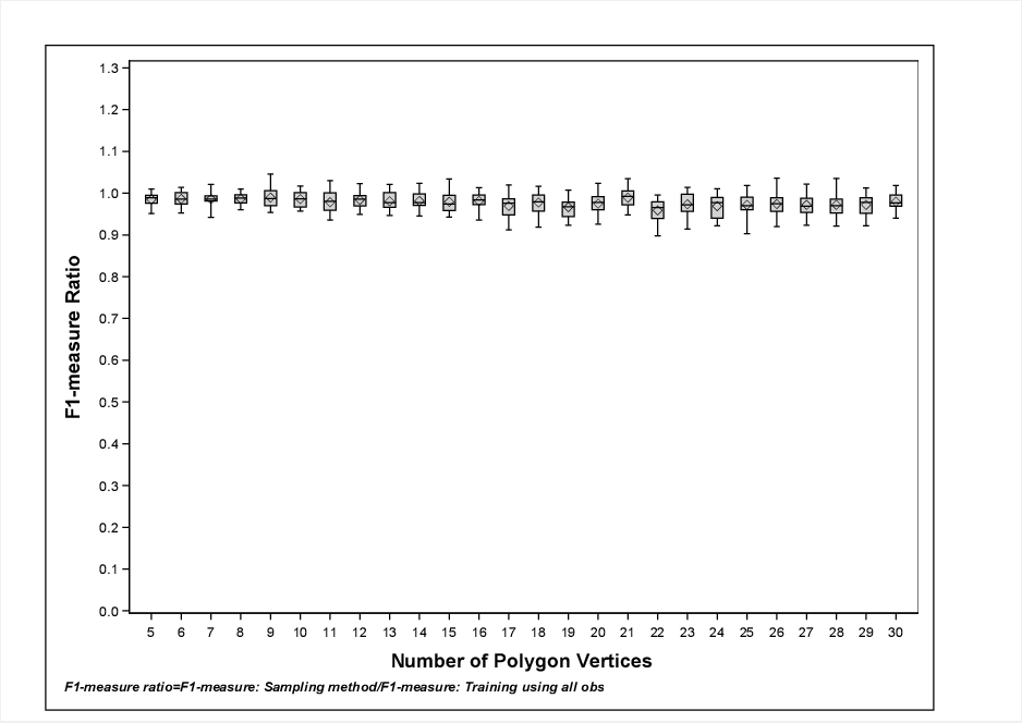
(a) $s$=1

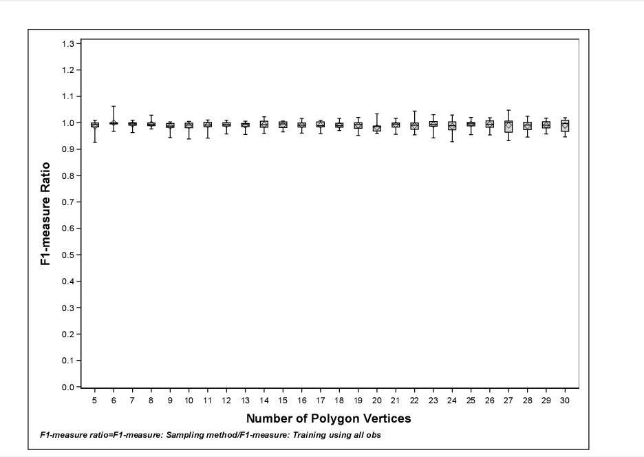
(b) $s$=1.4

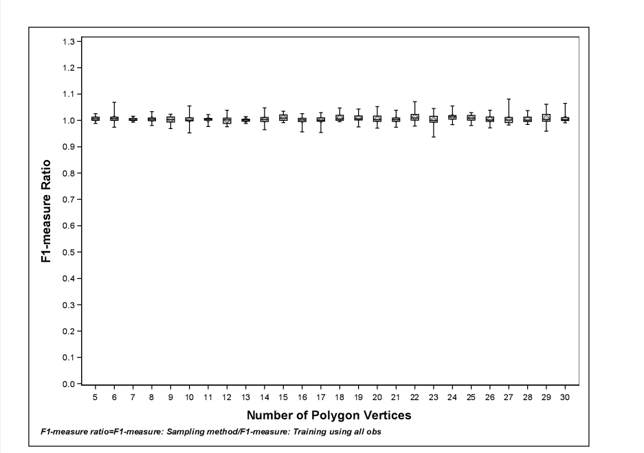
(c) $s$=2.3

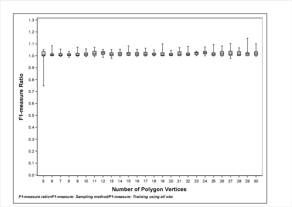
(d) $s$=3.4

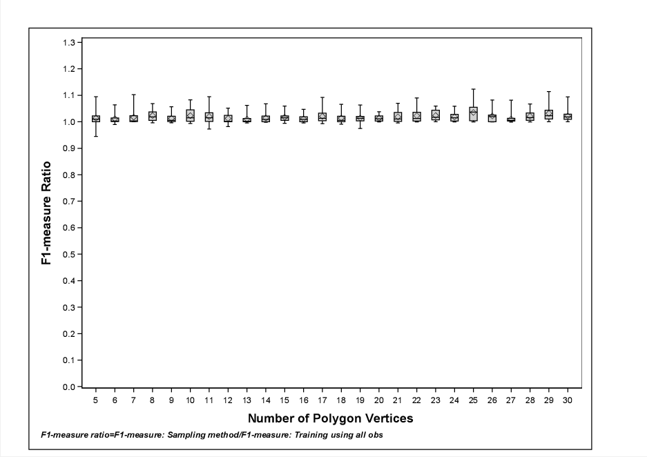
(e) $s$=4.1

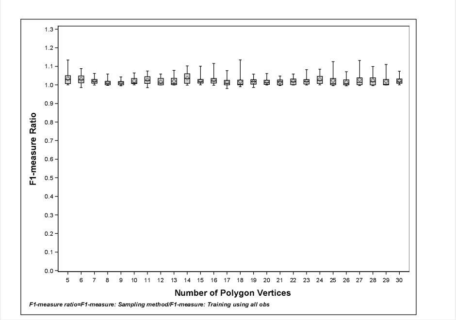
(f) $s$=5.0

Figure 14: Box-whisker plot: Number of vertices vs. $F_{1}$ measure ratio for different s values

VI-C Overall Results

Figure 15 provides summary of all simulation performed for different polygon instances and varying values of $s$. The plot shows that except for one outlier result, $F_{1}$-measure ratio is greater than 0.9 across number of vertice. The $F_{1}$ measure ratio in the top three quartiles is greater than $\approx 0.98$ across all values of the number of vertices. The accuracy of sampling method is comaprable to full SVDD method.

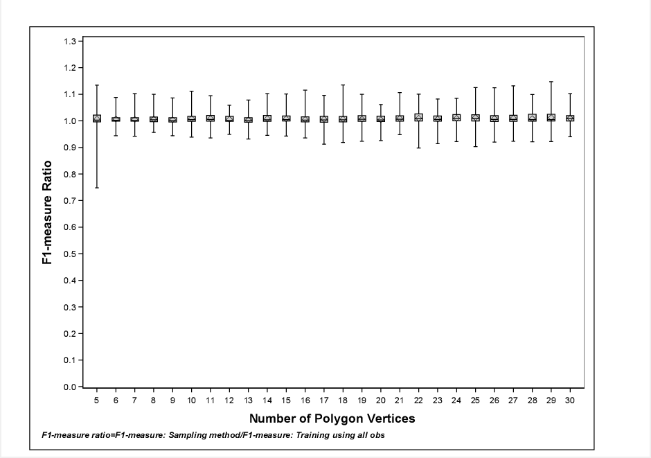
Figure 15: Box-whisker plot: Number of vertices vs. $F_{1}$ measure ratio

VII Conclusion

We propose a simple sampling-based iterative method for training SVDD. The method incrementally learns during each iteration by utilizing information contained in the current master set of support vectors and new information provided by the random sample. After a certain number of iterations, the threshold $R^{2}$ value and the center $a$ start to converge. At this point, the SVDD of the master set of support vectors is close to the SVDD of training data set. We provide a mechanism to detect convergence and establish a stopping criteria. The simplicity of proposed method ensures ease of implementation. The implementation involves writing additional code for calling SVDD training code iteratively, maintaining a master set of support vectors and implementing convergence criteria based on threshold $R^{2}$ and center $a$. We do not propose any changes to the core SVDD training algorithm as outlined in section I-A. The method is fast. The number of observations used for finding the SVDD in each iteration can be a very small fraction of the number of observations in the training data set. The algorithm provides good results in many cases with sample size as small as $m+1$, where $m$ is the number of variables in the training data set. The small sample size ensures that each iteration of the algorithm is extremely fast. The proposed method provides a fast alternative to traditional SVDD training method which uses information from all observations in one iteration. Even though the sampling based method provides an approximation of the data description but in applications where training data set is large, fast approximation is often preferred to an exact description which takes more time to determine. Within the broader realm of Internet of Things (IoT) we expect to see multiple applications of SVDD especially to monitor industrial processes and equipment health and many of these applications will require fast periodic training using large data sets. This can be done very efficiently with our method.

References

- [1] Anonymous github account with a sample based svdd implementation in python. https://github.com/samplesvdd/sample_svdd.
- [2] Chih-Chung Chang and Chih-Jen Lin. Libsvm: a library for support vector machines. ACM Transactions on Intelligent Systems and Technology (TIST), 2(3):27, 2011.
- [3] James J Downs and Ernest F Vogel. A plant-wide industrial process control problem. Computers & chemical engineering, 17(3):245–255, 1993.
- [4] Gul Ege. Multi-stage modeling delivers the roi for internet of things. http://blogs.sas.com/content/subconsciousmusings/2015/10/09/multi-stage-modeling-delivers-the-roi-for-internet-of-things/-…-is-epub/, 2015.
- [5] Pyo Kim, Hyung Chang, Dong Song, and Jin Choi. Fast support vector data description using k-means clustering. Advances in Neural Networks–ISNN 2007, pages 506–514, 2007.
- [6] M. Lichman. UCI machine learning repository, 2013.
- [7] Jian Luo, Bo Li, Chang-qing Wu, and Yinghui Pan. A fast svdd algorithm based on decomposition and combination for fault detection. In Control and Automation (ICCA), 2010 8th IEEE International Conference on, pages 1924–1928. IEEE, 2010.
- [8] F. Pedregosa, G. Varoquaux, A. Gramfort, V. Michel, B. Thirion, O. Grisel, M. Blondel, P. Prettenhofer, R. Weiss, V. Dubourg, J. Vanderplas, A. Passos, D. Cournapeau, M. Brucher, M. Perrot, and E. Duchesnay. Scikit-learn: Machine learning in Python. Journal of Machine Learning Research, 12:2825–2830, 2011.
- [9] N. Lawrence Ricker. Tennessee eastman challenge archive, matlab 7.x code, 2002. [Online; accessed 4-April-2016].
- [10] Carolina Sanchez-Hernandez, Doreen S Boyd, and Giles M Foody. One-class classification for mapping a specific land-cover class: Svdd classification of fenland. Geoscience and Remote Sensing, IEEE Transactions on, 45(4):1061–1073, 2007.
- [11] Thuntee Sukchotrat, Seoung Bum Kim, and Fugee Tsung. One-class classification-based control charts for multivariate process monitoring. IIE transactions, 42(2):107–120, 2009.
- [12] David MJ Tax and Robert PW Duin. Support vector data description. Machine learning, 54(1):45–66, 2004.
- [13] Achmad Widodo and Bo-Suk Yang. Support vector machine in machine condition monitoring and fault diagnosis. Mechanical Systems and Signal Processing, 21(6):2560–2574, 2007.
- [14] Alexander Ypma, David MJ Tax, and Robert PW Duin. Robust machine fault detection with independent component analysis and support vector data description. In Neural Networks for Signal Processing IX, 1999. Proceedings of the 1999 IEEE Signal Processing Society Workshop., pages 67–76. IEEE, 1999.
- [15] Ling Zhuang and Honghua Dai. Parameter optimization of kernel-based one-class classifier on imbalance learning. Journal of Computers, 1(7):32–40, 2006.