Improved sampling and validation of frozen Gaussian approximation with surface hopping algorithm for nonadiabatic dynamics

Abstract

In the spirit of the fewest switches surface hopping, the frozen Gaussian approximation with surface hopping (FGA-SH) method samples a path integral representation of the non-adiabatic dynamics in the semiclassical regime. An improved sampling scheme is developed in this work for FGA-SH based on birth and death branching processes. The algorithm is validated for the standard test examples of non-adiabatic dynamics.

I Introduction

The surface hopping algorithms, pioneered in Tully and Preston (1971) and revamped as the fewest switches surface hopping (FSSH) algorithm in Tully (1990), are widely used for mixed quantum-classical dynamics in the non-adiabatic regime. The surface hopping algorithms have been successfully applied to various scenarios where non-adiabatic effect is important Hammes-Schiffer and Tully (1994); Barbara et al. (1996); Tully (1998); Kapral (2006); Shenvi et al. (2009); Barbatti (2011); Subotnik et al. (2016). Due to the huge popularity, the development of surface hopping algorithms, which focuses on improving the approximation to the exact quantum dynamics, further reducing the computational cost, or taking into account the interaction with environment, just to name a few, has been a very active research area Hammes-Schiffer and Tully (1994); Barbara et al. (1996); Prezhdo and Rossky (1997); Tully (1998); Horenko et al. (2002); Jasper et al. (2002); Wu and Herman (2005); Bedard-Hearn et al. (2005); Hanna and Kapral (2005); Kapral (2006); Wu and Herman (2006, 2007); Hanna et al. (2007); Schmidt et al. (2008); Shenvi et al. (2009); Barbatti (2011); Subotnik and Shenvi (2011); Landry and Subotnik (2011); Gorshkov et al. (2013); Subotnik et al. (2013); Landry et al. (2013); Hanna and Kapral (2013); Jain et al. (2015); Jain and Subotnik (2015); Subotnik et al. (2016); Kapral (ress).

The underlying idea of the surface hopping algorithms is to use classical trajectories with hopping between adiabatic energy surfaces to approximate the exact Schrödinger dynamics, which is impractical to solve directly due to the curse of dimensionality. While the intuition behind the FSSH type algorithm is quite convincing, the understanding of its systematic derivation from the exact Schrödinger dynamics remains rather poor, despite huge progress in recent years Herman (1984); Kapral and Ciccotti (1999); Horenko et al. (2002); Hanna and Kapral (2005); Wu and Herman (2005, 2006); Kapral (2006); Gorshkov et al. (2013); Subotnik et al. (2013, 2016); Kapral (ress)

In our previous work Lu and Zhou (2016), we gave a mathematically rigorous derivation of a surface hopping type algorithm, called frozen Gaussian approximation with surface hopping (FGA-SH), starting from the nuclei-electron Schrödinger equation in the non-adiabatic regime. The algorithm can be viewed as a natural extension of the Herman-Kluk propagator Herman and Kluk (1984); Kay (1994, 2006), which is a consistent approximation to the single surface Schrödinger equation in the semiclassical regime, to the non-adiabatic dynamics and hence takes into account hopping between different energy surfaces.

The key observation behind the FGA-SH method is that the idea of surface hopping leads to a path integral representation of the semiclassical Schrödinger equations for multiple adiabatic surfaces (referred to as the matrix Schrödinger equation in the sequel), for which the path is given by the classical paths with hops between adiabatic surfaces, in the same spirit of those used in FSSH. To prevent any possible confusion, we emphasize that this is rather different from the Feynman path integral, in particular, the paths are similar to those trajectories of nuclei in FSSH and paths may carry different weights. This path integral representation not only provides a clear interpretation of the FSSH type algorithms in terms of a Monte Carlo sampling scheme of the path integral, but also naturally leads to further improvement of numerical schemes to approximate the path integral, which the current work is devoted to.

The main new ingredient of the improved algorithm in this work is that instead of using independent trajectories (as a direct Monte Carlo sampling scheme), we reduce the sampling variance by adopting the birth-death branching processes, which is typically used in other context of path integral sampling, e.g., the diffusion Monte Carlo algorithms Grimm and Storer (1969, 1971); Anderson (1975). As far as we know, this is the first time such strategy is used for surface hopping type algorithms, thanks to the novel path integral interpretation. In fact, we expect the connection of the view point of surface hopping algorithms with the path integral based methods (see e.g., Cao and Voth (1994); Sun and Miller (1997); Jang and Voth (1999); Makri (1999); Miller (2001); Craig and Manolopoulos (2004); Lambert and Makri (2012); Habershon et al. (2013)) would be quite fruitful and would fertilize better algorithms for non-adiabatic dynamics. The birth-death branching processes result in an adaptive pruning and splitting of surface hopping trajectories, which bears some similarity with the multiple spawning method Martinez et al. (1996); Ben-Nun and Martinez (1998) in the context of non-adiabatic dynamics, while the latter spawns Gaussian as a set of basis functions for a wave function approach, rather than semiclassical trajectories.

Besides the improved sampling scheme of FGA-SH, in this work we also further elaborate the initial sampling of trajectories in the FGA-SH method and also the calculation of observables based on averaging of trajectories. We validate the improved FGA-SH method by various numerical tests, which explore the dependence of the numerical error on the semiclassical parameter $\varepsilon$, the long time accuracy and conservation of energy, the impact of the weighting factor, etc. for the model test problems by Tully Tully (1990) for nonadiabatic dynamics.

The rest of the paper is organized as follows. In Section II, we review the path integral representation for matrix Schrödinger equation in the semiclassical regime which leads to the FGA-SH method introduced in Lu and Zhou (2016). The improved sampling algorithm for FGA-SH is discussed in Section III. We validate the method by numerical tests in Section IV. The paper is concluded in Section V.

II Theory

II.1 Path integral representation for semiclassical matrix Schrödinger equations

We consider the matrix Schrödinger equation with two electronic levels in the adiabatic basis:

$$i\varepsilon\partial_{t}\begin{pmatrix}u_{0}\\ u_{1}\end{pmatrix}=-\frac{\varepsilon^{2}}{2}\Delta_{x}\begin{pmatrix}u_{0}\\ u_{1}\end{pmatrix}+\begin{pmatrix}E_{0}\\ &E_{1}\end{pmatrix}\begin{pmatrix}u_{0}\\ u_{1}\end{pmatrix}\\ -\frac{\varepsilon^{2}}{2}\begin{pmatrix}D_{00}&D_{01}\\ D_{10}&D_{11}\end{pmatrix}\begin{pmatrix}u_{0}\\ u_{1}\end{pmatrix}-\varepsilon^{2}\sum_{j=1}^{m}\begin{pmatrix}d_{00}&d_{01}\\ d_{10}&d_{11}\end{pmatrix}_{j}\partial_{x_{j}}\begin{pmatrix}u_{0}\\ u_{1}\end{pmatrix},$$ (1)

where for $k,l=0,1,\;j=1,\ldots,m$,

$$D_{kl}(x)=\langle\Psi_{k}(r;x),\Delta_{x}\Psi_{l}(r;x)\rangle_{r},$$ (2)

$$\left(d_{kl}(x)\right)_{j}=\langle\Psi_{k}(r;x),\partial_{x_{j}}\Psi_{l}(r;x)\rangle_{r}.$$ (3)

Here $m$ is the spatial dimension of the nuclei degree of freedom $x$ and $\Psi_{k}(r;x)$ are adiabatic states where $r$ denotes the electronic degree of freedom. Note that our index convention of $D_{kl}$ and $d_{kl}$ is flipped from that of Tully Tully (1990), we choose the current convention so that the terms in (1) follows the usual index convention of matrix-vector product.

The matrix Schrödinger equation is obtained from the nuclei-electron Schrödinger equation by expanding the total wave function in the adiabatic basis. After rescaling, the semiclassical nuclei-electron Schrödinger equation reads (see e.g., Hagedorn (1986); Panati et al. (2007))

$$i\varepsilon\partial_{t}\Phi(t,x,r)=-\frac{\varepsilon^{2}}{2}\Delta_{x}\Phi(t,x,r)+H_{e}(r,x)\Phi(t,x,r),$$ (4)

where $\Phi(t,x,r)$ denotes the nuclei-electron wave function and $H_{e}(r,x)$ denotes electronic Hamiltonian (in a diabatic representation). The parameter $\varepsilon$ is proportional to the square root of the ratio of the electron mass to that of nuclei and is thus a small parameter (for simplicity of notation, we have assumed that all nuclei share the same mass). The adiabatic states $\Psi_{k}(r;x)$ are the eigenstates of $H_{e}(r,x)$ with eigenvalues $E_{k}(x)$. Assume the first two adiabatic states are well isolated from the rest of the states, we thus take the following ansatz for the total wave function

$$\Phi(t,x,r)=u_{0}(t,x)\Psi_{0}(r;x)+u_{1}(t,x)\Psi_{1}(r;x).$$ (5)

We obtain (1) by inserting (5) into (4) and writing the equations in terms of $u_{0}$ and $u_{1}$. While it is possible to generalize the method to take into account of more than two adiabatic surfaces, we restrict to the case of two for simplicity.

Solving the matrix Schödinger equations (1) using conventional numerical methods is impractical due to the potential high dimensionality of the nuclei degree of freedom, and hence we resort to semiclassical methods which exploit the limiting behavior of $\varepsilon\to 0$. In previous work Lu and Zhou (2016), we derived the frozen Gaussian approximation with surface hopping (FGA-SH) from the matrix Schrödinger equation with rigorous error bounds of the approximate nuclei wave function. The algorithm follows the same spirit as the Tully’s fewest switches surface hopping (FSSH) method Tully (1990), except that the hopping rule is different from FSSH, as will be explained in subsection II.2.

The FGA-SH method can be understood as a path integral formulation of the matrix Schrödinger equation in the spirit of surface hopping. It approximates the solution $u=\bigl{(}\begin{smallmatrix}u_{0}\\ u_{1}\end{smallmatrix}\bigr{)}$ as

$$u(T,x) =u_{\text{FGA-SH}}(T,x)+\mathcal{O}(\varepsilon)$$ (6)

$$=\mathbb{E}_{\widetilde{z}}\mathcal{F}\bigl{(}x;\{\widetilde{z}(s)\}_{0\leq s\leq T}\bigr{)}+\mathcal{O}(\varepsilon),$$

where the average is taken over an ensemble of trajectories we describe below in Section II.2 and the functional $\mathcal{F}$ (expression given below in Section II.3) depends on the trajectory $\widetilde{z}$ up to time $T$. Our surface hopping algorithm can be viewed as a Monte Carlo sampling scheme for this path integral. As proved in Lu and Zhou (2016), $u_{\text{FGA-SH}}$ gives an approximation to the exact solution with error $\mathcal{O}(\varepsilon)$ (in $L^{2}$ metric) for any finite $T$. For completeness, we provide in the Appendix a brief discussion of the derivation of (6). The readers may refer to Lu and Zhou (2016) for detailed asymptotic derivation.

II.2 Surface hopping trajectories

Let us first specify the ensemble of trajectories used in (6), which largely follows the spirit of surface hopping trajectories. The trajectory $\widetilde{z}(t)$ in (6) evolves on the extended phase space which consists of the classical phase space on two energy surfaces: we write $\widetilde{z}(t)=(z(t),l(t))\in{\mathbb{R}}^{2m}\times\{0,1\}$, where $l(t)\in\{0,1\}$ indicates the energy surface that the trajectory lies on at time $t$. The position and momentum $z(t)=(p(t),q(t))$ evolves by a Hamiltonian flow on the energy surface $l(t)$:

$$\begin{cases}&\dot{q}(t)=p(t);\\ &\dot{p}(t)=-\nabla_{q}E_{l(t)}(q(t)).\end{cases}$$ (7)

The trajectory hops between surfaces according to a Markov jump process, with infinitesimal transition rate over the time period $(t,t+\delta t)$:

$$\mathbb{P}\bigl{(}l(t+\delta t)=m\mid l(t)=n,\,z(t)=z\bigr{)}=\delta_{nm}+\lambda_{nm}(z)\delta t+o(\delta t)$$ (8)

for $m,n\in\{0,1\}$, where the rate matrix is given by

$$\begin{pmatrix}\lambda_{00}(z)&\lambda_{01}(z)\\ \lambda_{10}(z)&\lambda_{11}(z)\end{pmatrix}=\begin{pmatrix}-\left\lvert p\cdot d_{10}(q)\right\rvert&\left\lvert p\cdot d_{10}(q)\right\rvert\\ \left\lvert p\cdot d_{01}(q)\right\rvert&-\left\lvert p\cdot d_{01}(q)\right\rvert\end{pmatrix}.$$ (9)

That is, if the trajectory is on the surface $0$ at time $t$, then during the time interval $(t,t+\delta t)$, the probability that the trajectory hops to the surface $1$ is given by $\lvert p(t)\cdot d_{10}(q(t))\rvert\delta t$ for sufficiently small $\delta t$. We remark that $p\cdot d_{10}(q)$ is in general complex, and hence we take its modulus in the rate matrix; also note that the rate is state dependent (on $z(t)$). The trajectory $\widetilde{z}(t)$ thus follows a Markov switching process, which is piecewise deterministic. The sampled trajectories follow the Hamiltonian dynamics on each energy surface, with random hops to the other energy surfaces, and thus are very similar in spirit to those trajectories used in the FSSH method (though with different hopping rules).

According to (7), the position and momentum part $z(t)=(p(t),q(t)$) of the trajectory $\widetilde{z}(t)$ is continuous and piecewise differentiable, while $l(t)$ is piecewise constant with almost surely finite many jumps during any finite time interval. Given a realization of the trajectory $\widetilde{z}(t)=(z(t),l(t))$ starting from initial condition $\widetilde{z}(0)=(z(0),l(0))$, we denote by $n$ the number of jumps $l(t)$ has in the time interval $[0,T]$ (thus $n$ is a random variable) and also the discontinuity set of $l(t)$ as $\bigl{\{}t_{1},\cdots,t_{n}\bigr{\}}$, which is an increasingly ordered random sequence. At each of those time, the trajectory switches from one energy surface to the other; and thus $t_{k}$, $k=1,\ldots,n$, are referred to as hopping times in the sequel.

The starting point of the trajectory $\widetilde{z}(0)=(z(0),l(0))$ is sampled according to a distribution on the extended phase space determined by the initial condition of the matrix Schrödinger equation. Given the initial wave function $u_{k}(0,x)$ for $k=0,1$, we denote the Gaussian packet transform of $u$ as

$$A_{0}(z,l)=2^{\frac{m}{2}}\int_{{\mathbb{R}}^{m}}u_{l}(0,y)e^{\frac{i}{\varepsilon}(-p_{0}\cdot(y-q)+\frac{i}{2}|y-q|^{2})}\,\mathrm{d}y.$$ (10)

Then the $\widetilde{z}(0)=(z(0),l(0))$ is sampled from the measure $\mathbb{P}_{0}(z(0),l(0))$ with probability density on ${\mathbb{R}}^{2m}\times\{0,1\}$ proportional to $\lvert A_{0}(z(0),l(0))\rvert$. Here we assume that $A_{0}(\cdot,k)$ is integrable on ${\mathbb{R}}^{2m}$ for each $k=0,1$ and we denote the normalizing factor as

$$\mathcal{Z}_{0}=\frac{1}{(2\pi\varepsilon)^{3m/2}}\sum_{k=0,1}\int_{{\mathbb{R}}^{2m}}\left\lvert A_{0}(z,k)\right\rvert\,\mathrm{d}z.$$ (11)

Thus, the initial point of the trajectory $\widetilde{z}(t)$ follows the distribution

$$\mathbb{P}_{0}(z,l)=\mathcal{Z}_{0}^{-1}\frac{1}{(2\pi\varepsilon)^{3m/2}}\lvert A_{0}(z,l)\rvert.$$ (12)

We will discuss the numerical sampling of initial points in Section III.2.

II.3 Ensemble average of surface hopping trajectories

Given the description of the ensemble of paths $\widetilde{z}(t)$, $t\in[0,T]$, we now specify the functional $\mathcal{F}$ in the path integral (6). Recall that we denote $n$ the number of hops of the trajectory and $\bigl{\{}t_{1},\cdots,t_{n}\bigr{\}}$ the sequence of hopping times. For convenience, we also denote $t_{0}=0$ and $t_{n+1}=T$, the starting and final time of the trajectory. The functional $\mathcal{F}$ is then given by

$$\mathcal{F}\bigl{(}x;\{\widetilde{z}(t)\}_{0\leq t\leq T}\bigr{)}=\lvert l(T)\rangle\,\frac{\mathcal{Z}_{0}}{\left\lvert A_{0}(\widetilde{z}(0))\right\rvert}A(T)\times\\ \times\exp\Bigl{(}\frac{i}{\varepsilon}\Theta(T,x)\Bigr{)}\exp\Bigl{(}w(T)\Bigr{)}\prod_{k=1}^{n}\frac{\tau^{(k)}}{\left\lvert\tau^{(k)}\right\rvert}\,,$$ (13)

where $\lvert 0\rangle=\bigl{(}\begin{smallmatrix}1\\ 0\end{smallmatrix}\bigr{)}$ and $\lvert 1\rangle=\bigl{(}\begin{smallmatrix}0\\ 1\end{smallmatrix}\bigr{)}$ denotes the electronic state associated with each surface, $\mathcal{Z}_{0}$ is defined in (11), $A_{0}(\widetilde{z}(0))=A_{0}(z(0),l(0))$ is given in (10), and all the other terms depend on the trajectory, in particular, the sequence of hopping times (we suppress the dependence in the notation for simplicity). An outline of the argument leading to (13) is provided in the Appendix, with the detailed asymptotic derivation provided in Lu and Zhou (2016). It comes from a stochastic representation of a high dimensional integral involving all possible hopping times of a surface hopping trajectory.

Let us explain the terms appeared in (13). $\lvert l(T)\rangle$ gives the electronic state of the trajectory at time $T$, and the factor $\mathcal{Z}_{0}/\lvert A_{0}(\widetilde{z}(0))\rvert$ results from the initial sampling. The term

$$A(T)\exp\Bigl{(}\frac{i}{\varepsilon}\Theta(T,x)\Bigr{)}$$

resembles the familiar amplitude $(A(T))$ and phase $(\Theta(T,x))$ expression from the Herman-Kluk propagator Herman and Kluk (1984); Kay (1994, 2006); Swart and Rousse (2009), in particular, the phase term $\Theta$ takes the following form

$$\Theta(t,x)=S(t)+\frac{i}{2}\lvert x-q(t)\rvert^{2}+p(t)\cdot(x-q(t)),$$ (14)

where $S(t)$ is the classical action associated with the trajectory and recall that $z(t)=(p(t),q(t))$ is the momentum and position of the trajectory. The amplitude $A$ and action $S$ solve the ODEs

$$\dot{S}(t) =\frac{1}{2}p(t)^{2}-E_{l(t)}(q(t)),$$ (15)

$$\dot{A}(t) =\frac{1}{2}A\operatorname{tr}\Bigl{(}Z(t)^{-1}\bigl{(}\partial_{z}p(t)-i\partial_{z}q(t)\nabla^{2}_{q}E_{l(t)}(q(t))\bigr{)}\Bigr{)}$$

$$\quad-A\,d_{l(t)l(t)}(q(t))\cdot p(t).$$ (16)

with initial conditions $S(0;\widetilde{z}(0))=0$ and $A(0;\widetilde{z}(0))=A_{0}(\widetilde{z}(0))$. Here $\partial_{z}$ is short for $\partial_{z}=\partial_{q(0)}-i\partial_{p(0)}$ and $Z(t)=\partial_{z}(q(t)+ip(t))$. Those equations are similar to the evolution equations in Herman-Kluk propagator, except that similar to the evolution equations for $(p(t),q(t))$, the above ODEs also depend on the current surface $l(t)$ of the trajectory. Also note that it is clear for the ODEs that the value $S(t)$ and $A(t)$ are determined by the trajectory up to time $t$.

The last term in (13) involves the hopping coefficients $\tau^{(k)}$ at each hopping, given by

$$\tau^{(k)}=-p(t_{k})\cdot d_{l(t_{k}^{+})l(t_{k}^{-})}(q(t_{k})),$$ (17)

where $l(t_{k}^{-})$ and $l(t_{k}^{+})$ give the energy surface index before and after the hop at hopping time $t_{k}$ (so that $l(t_{k}^{-})\neq l(t_{k}^{+})$). Recall that this is exactly related to the jumping intensity used for surface hopping of the trajectories. Since $\tau^{(k)}$ is complex valued in general, we have chosen its modulus as the jumping intensity $\lambda$ in the surface hopping trajectory, the term $\tau^{(k)}/\left\lvert\tau^{(k)}\right\rvert$ in (13) is used to correct the phase factor due to the complex value.

Finally, the weighting factor $w$ in (13) solves the ODE

$$\dot{w}(t)=\left\lvert p(t)\cdot d_{(1-l(t))l(t)}(q(t))\right\rvert,$$ (18)

with initial condition $w(0)=0$. Thus, it is the accumulated jumping intensity of the trajectory. The appearance of the weighting term in (13) is due to the fact that the infinitesimal transition rate (8) of the trajectory $\widetilde{z}$ is non-homogeneous and depends on the current position and momentum. Therefore, we need to reweight the terms in the path-integral representation such that the average gives the correct wave function. Without the weighting term, the path integral formulation is no longer an accurate approximation Lu and Zhou (2016); we also show in Section IV.4 the crucial role of such weighting terms for calculating observables associated to the non-adiabatic dynamics.

For the algorithmic purpose, we remark that we can combine $A$ with the weighting factor $w$ as

$$\Gamma(t)=\frac{A(t)}{|A(0)|}\exp\bigl{(}w(t)\bigr{)},$$ (19)

which solves the ODE

$$\dot{\Gamma}(t)=\frac{1}{2}\Gamma\operatorname{tr}\Bigl{(}Z(t)^{-1}\bigl{(}\partial_{z}p(t)-i\partial_{z}q(t)\nabla^{2}_{q}E_{l(t)}(q(t))\bigr{)}\Bigr{)}\\ +\Gamma\Bigl{(}\left\lvert p(t)\cdot d_{(1-l(t))l(t)}(q(t))\right\rvert-p(t)\cdot d_{l(t)l(t)}(q(t))\Bigr{)}$$ (20)

with initial condition $\Gamma(0;\widetilde{z}(0))=A_{0}(\widetilde{z}(0))/|A_{0}(\widetilde{z}(0))|$. The quantity $\left\lvert\Gamma(t)\right\rvert$ will be treated as the weight of the trajectory in our algorithm. Thus we will prune trajectories with small weight, and branch trajectories with larger weights to reduce the variance of the stochastic sampling algorithm.

III Algorithm

III.1 FGA-SH sampling based on birth/death branching process

As discussed before, the path integral representation readily suggests a direct Monte Carlo sampling strategy: An ensemble of independent trajectories are generated as in section II.2 and then the average of $\mathcal{F}$ is calculated as in section II.3 to approximate the time-dependent wave function or the associated observables. This is the algorithm used in our previous work Lu and Zhou (2016). Here we present an improved sampling strategy based on birth/death branching process to reduce the sampling variance of the ensemble average, borrowing a familiar variance reduction method in the context of diffusion Monte Carlo algorithms. The basic idea is to prune the trajectories with small weights, while duplicate those with larger weights ($\lvert\Gamma(t)\rvert$), in a consistent way that the mean is preserved, while avoiding few trajectories carry huge weights so to reduce the variance of the sampling. Note that the trajectories are no longer independent, the dependence comes in due to the branching step.

The algorithm starts by sampling a collection of initial points for the trajectories and estimate $\mathcal{Z}_{0}$ defined in (11), which will be discussed in more details in section III.2. We denote by $M(0)$ the number of trajectories initially. Each trajectory carries the information of position $q_{\alpha}$, momentum $p_{\alpha}$, the index of energy surface $l_{\alpha}$, classical action $S_{\alpha}$, and a weight $\gamma_{\alpha}$; initially we set $S_{\alpha}=0$ and $\gamma_{\alpha}=A_{0}(\widetilde{z}_{\alpha}(0))/|A(\widetilde{z}_{\alpha}(0))|$ for each trajectory. We use $\gamma_{\alpha}$ here to distinguish with $\Gamma$ since during the branching process, the weight $\gamma_{\alpha}$ of a trajectory will be redistributed among the offspring and hence differ from $\Gamma$, as will be discussed in the algorithm below.

The propagation of the trajectories are carried out as follows: For each time step of size $\Delta t$, the following steps are performed in order:

1. Evolve the position and momentum $p(t),q(t)$ by the Hamiltonian dynamics (7) on the current surface $l(t)$ for time interval $\Delta t$ for each trajectory (we omit the index of trajectory in the algorithm description for simplicity of notation).

2. Evolve the quantities $S$ and $\gamma$ following (15) and (20) respectively according to the current surface of the trajectory $l(t)$. Note that as discussed in section II.3, the quantities $S$ and $\gamma$ at time $t$ only depend on the portion of the trajectory $\widetilde{z}$ up to time $t$. Therefore we may calculate them for each trajectory on the fly. These ODEs can be numerically solved by standard ODE integrators, for example, a $4$-th order Runge-Kutta scheme is chosen in our implementation.

3. Hopping attempts. The probability that a surface hop occurs within the time interval $(t,t+\Delta t)$ is given by $\Delta t\lvert\lambda_{(1-l(t))l(t)}\rvert$. For $\Delta t$ sufficiently small, we can neglect the event that two hops happen within the time interval. With this probability, the trajectory is hopped to the other surface, so that the label of the energy surface is changed: $l(t+\Delta t)=1-l(t)$ and the phase change $\tau/\lvert\tau\rvert$ is recorded.

4. Birth/death branching. For every $N_{\text{branch}}$ steps we do the branching according to the weight that the trajectories carry at time $t+\Delta t$: $\gamma=\gamma(t+\Delta t)$. For each trajectory, we generate a random number $\xi$ uniformly distributed on $[0,1]$. Denoting $[\lvert\gamma\rvert]$ as the integer part of $\lvert\gamma\rvert$, the birth/death is given by

   • If $\xi>\lvert\gamma\rvert-[\lvert\gamma\rvert]$, we replace the current trajectory with $[\lvert\gamma\rvert]+1$ trajectories identical to the parent trajectory except that the weight is reset to be $\gamma/|\gamma|$;

   • If $\xi\leq\lvert\gamma\rvert-[\lvert\gamma\rvert]$, we replace the current trajectory with $[\lvert\gamma\rvert]$ trajectories identical to the parent trajectory except that the weight is reset to be $\gamma/|\gamma|$. If $[\lvert\gamma\rvert]=0$, this means that we kill the parent trajectory without any offsprings.

   Note that the branching rule is designed so that on average the total weight of the offsprings is equal to the weight of the parent trajectory, whereas the weight of each offspring is of order $1$.

After propagating the trajectories till $t=T$, the wave function can be reconstructed following (6) with the modification to take into account the birth/death branching process. The path integral is approximated by

$$u_{\text{FGA-SH}}(T,x)=\frac{\mathcal{Z}_{0}}{M(0)}\sum_{\alpha=1}^{M(T)}\lvert l_{\alpha}(T)\rangle\,\gamma_{\alpha}(T)\times\\ \times\exp\Bigl{(}\frac{i}{\varepsilon}\Theta_{\alpha}(T,x)\Bigr{)}\prod_{k=1}^{n_{\alpha}}\frac{\tau_{\alpha}^{(k)}}{\left\lvert\tau_{\alpha}^{(k)}\right\rvert},$$ (21)

where $M(T)$ denotes the number of trajectory at time $T$ and we use subscript $\alpha$ explicitly to emphasize the dependence of these quantities on the right hand side on each trajectory. We also remark that $|\gamma_{\alpha}|\approx 1$ due to the branching process, so it mainly contributes to a phase factor in the summation.

We emphasize that, except for the step of birth/death branching, these is no exchange of information between the trajectories, and moreover, the branching history does not contribute to the modified average of trajectories (21), and is hence not necessary to be stored. Therefore, the computational cost to generate one trajectory in the current algorithm is almost the same as those with fully independent trajectories, e.g., the direct Monte Carlo sampling of the path integral Lu and Zhou (2016).

III.2 Initial sampling

We now further elaborate the initial sampling of the trajectories. For simplicity, let us assume that initially, the wave function is only non-zero on surface $0$, so that the trajectories will all initiate on that surface. Recall that we aim to sample $z(0)$ according to the probability distribution

$$\mathbb{P}_{0}(q,p,0)=\frac{1}{\mathcal{Z}_{0}}\frac{1}{(2\pi\varepsilon)^{3m/2}}\left|A_{0}(z(0),0)\right|,$$ (22)

where $A_{0}$ is defined in (10) and $\mathcal{Z}_{0}$ in (11). We assume that $A_{0}(z(0),0)$ can be obtained with some accuracy. Explicit calculation is unfortunately only possible in low dimensions for general initial data, due to the curse of dimension in numerical quadrature. A special case is if we assume $u_{0}(y)$ is a Gaussian wave packet, for which $A_{0}$ and $\mathcal{Z}_{0}$ can be obtained explicitly. We now give the expression of $\mathbb{P}_{0}$ for Gaussian initial data, as this is used in our numerical tests. For example, if we consider a semiclassical wave packet centered at $y=\tilde{q}$ with momentum $\tilde{p}$,

$$u_{0}(y)=\exp\left(\frac{i}{\varepsilon}\tilde{p}\cdot(y-\tilde{q})\right)\exp\left(-\sum_{j=1}^{m}\frac{a_{j}}{2\varepsilon}(y_{j}-\tilde{q}_{j})^{2}\right),$$

where $a_{j}$ are positive constants. By direct calculation, we have

$$A_{0}(q,p,0)=2^{m}(\pi\varepsilon)^{\frac{m}{2}}\prod_{j=1}^{m}(1+a_{j})^{-\frac{1}{2}}\exp\left(-\frac{(\tilde{p}_{j}-p_{j})^{2}+a_{j}(\tilde{q}_{j}-q_{j})^{2}}{2(1+a_{j})\varepsilon}\right)\exp\left(\frac{i(a_{j}\tilde{q}_{j}+q_{j})(\tilde{p}_{j}-p_{j})}{(1+a_{j})\varepsilon}+\frac{i\left(p_{j}q_{j}-\tilde{p}_{j}\tilde{q}_{j}\right)}{\varepsilon}\right),$$ (23)

and thus

$$\left\lvert A_{0}(q,p,0)\right\rvert=2^{m}(\pi\varepsilon)^{\frac{m}{2}}\prod_{j=1}^{m}(1+a_{j})^{-\frac{1}{2}}\\ \times\exp\left(-\frac{(\tilde{p}_{j}-p_{j})^{2}+a_{j}(\tilde{q}_{j}-q_{j})^{2}}{2(1+a_{j})\varepsilon}\right).$$ (24)

The resulting probability distribution for the initial position and momentum is a multivariate normal distribution centered at $q=\tilde{q}$ and $p=\tilde{p}$ with standard derivation $\mathcal{O}(\sqrt{\varepsilon})$. The normalizing constant $\mathcal{Z}_{0}$ can be also calculated analytically as

$$\mathcal{Z}_{0}=\frac{1}{(2\pi\varepsilon)^{3m/2}}\int_{{\mathbb{R}}^{2m}}\left\lvert A_{0}(z,0)\right\rvert\,\mathrm{d}z=2^{\frac{m}{2}}\prod_{j=1}^{m}\left(\frac{1+a_{j}}{a_{j}}\right).$$

Therefore, the probability distribution (22) is obtained explicitly. In the special case that $a_{j}=1$, $\forall\,j$, we have $\mathcal{Z}_{0}=2^{m}$ and the initial probabilistic measure is given by

$$\mathbb{P}(p,q,0)=2^{-2m}(\varepsilon\pi)^{-m}\exp\left(-\frac{|\tilde{p}-p|^{2}+|\tilde{q}-q|^{2}}{4\varepsilon}\right).$$

The initial momentum and position of the trajectories $(p_{\alpha}(0),q_{\alpha}(0))$ are sampled independently from the distribution and we set $l_{\alpha}=0$, $S_{\alpha}=0$ and the initial weight

$$\gamma_{\alpha}=\frac{A_{0}(z_{\alpha}(0),0)}{|A_{0}(z_{\alpha}(0),0)|}.$$

For the Gaussian initial data, we can directly sample $(p,q)$ from $\mathbb{P}_{0}$, which is a Gaussian distribution on the phase space. For more general $\mathbb{P}_{0}$, some importance sampling might be needed, which we will not go into details here.

III.3 Computing observables

For many applications, the goal is not to approximate the wave function itself, but rather the time evolution of certain observable. For the purpose of calculating an observable, it is often the case that we do not need to reconstruct the wave function on a mesh, which is not feasible in high dimensions anyway.

We take the mass on each energy surface as an example, denoted by

$$m_{k}=\int_{{\mathbb{R}}^{m}}\left|{u_{k}}(T,x)\right|^{2}\,\mathrm{d}x,\quad k=0,1,$$ (25)

other macroscopic quantities can be treated in a similar fashion. From the approximation of the wave function in FGA-SH, we have

$$\left|{u_{k}}(T,x)\right|^{2}={u_{k}}(T,x)\bar{u}_{k}(T,x).$$

Using (21) for both $u_{k}$ and the complex conjugate $\bar{u}_{k}$, we arrive at

$$\left|{u_{k}}(T,x)\right|^{2} \approx\frac{\mathcal{Z}_{0}^{2}}{(M(0))^{2}}\sum_{\alpha,\beta=1}^{M(T)}\Biggl{[}\delta_{k,l_{\alpha}(T)}\delta_{k,l_{\beta}(T)}\gamma_{\alpha}\overline{\gamma_{\beta}}\times$$

$$\quad\times g_{\alpha,\beta}(x)\prod_{k=1}^{n_{\alpha}}\frac{\tau_{\alpha}^{(k)}}{\left\lvert\tau_{\alpha}^{(k)}\right\rvert}\prod_{k=1}^{n_{\beta}}\frac{\bar{\tau}_{\beta}^{(k)}}{\left\lvert\tau_{\beta}^{(k)}\right\rvert}\Biggr{]},$$ (26)

where $\alpha$ and $\beta$ are indices for two trajectories (for $u_{k}$ and $\bar{u}_{k}$ respectively), and we have use the short-hand notation

$$g_{\alpha,\beta}(x) =\exp\Bigl{(}\frac{i}{\varepsilon}\Theta_{\alpha}-\frac{i}{\varepsilon}\bar{\Theta}_{\beta}\Bigr{)}.$$

We remark that while the formula (26) appears to complex, the resulting $m_{k}$ is in fact real due to the symmetry of interchanging indices $\alpha$ and $\beta$.

We observe that the only dependence on $x$ of the right hand side of (26) is through $g_{\alpha,\beta}(x)$, and since it is a Gaussian function, the integration in $x$ can be carried out analytically:

$$\int_{{\mathbb{R}}^{m}}g_{\alpha,\beta}(x)\,\mathrm{d}x=(\pi\varepsilon)^{\frac{m}{2}}e^{\frac{i}{\varepsilon}(S_{\alpha}(t)-S_{\beta}(t))}\times\\ \times e^{-\frac{i}{2\varepsilon}(q_{\alpha}(t)-q_{\beta}(t))\cdot(p_{\alpha}(t)+p_{\beta}(t))}\times\\ \times e^{-\frac{1}{4\varepsilon}\lvert q_{\alpha}(t)-q_{\beta}(t)\rvert^{2}-\frac{1}{4\varepsilon}\lvert p_{\alpha}(t)-p_{\beta}(t)\rvert^{2}},$$

Therefore, given the sampled FGA-SH trajectories (and hence $p_{\alpha}(t),q_{\alpha}(t)$ etc.), we can estimate $m_{k}$ without reconstruction and numerical quadrature of the wave functions.

IV Results and discussions

IV.1 Tully’s three examples

We now revisit the standard models examples similar to those of Tully’s Tully (1990), which are test cases widely used for non-adiabatic dynamics. The algorithm is not limited to one dimension, the comparison for higher dimensional systems (for instance the spin-boson system) will be considered in future works. All the examples below have two adiabatic states, which means that the Hilbert space corresponding to the electronic degree of freedom is equivalent to ${\mathbb{C}}^{2}$, and hence the electronic Hamiltonian $H_{e}$ (in a diabatic representation) is equivalent to a $2\times 2$ matrix.

Example 1. Simple avoided crossing.

For the simple avoided crossing example, we will vary the energy gap (controlled by the small parameter $\delta$) between the two surfaces as $\varepsilon\to 0$, which is a more interesting scenario. For this, we consider a class of electronic Hamiltonian given by a product of a scalar function $F^{\delta}(x)$ and a $2\times 2$ matrix $M(x)$ independent of $\delta$, namely

$$H_{e}^{\delta}(x)=F^{\delta}(x)M(x).$$

Since $F^{\delta}$ is a scalar, $H_{e}^{\delta}$ and $M$ share the same eigenfunctions. Denoting the eigenvalues of $M$ by $\lambda_{k}$, we have

$$E_{k}^{\delta}(x)=F^{\delta}(x)\lambda_{k}(x).$$ (27)

Then, we obtain that, for $k\neq l$,

$$d^{\delta}_{lk}=\frac{\langle\Psi_{l},\nabla_{x}H_{e}^{\delta}\Psi_{k}\rangle}{E_{k}^{\delta}-E_{l}^{\delta}}=\frac{\langle\Psi_{l},\nabla_{x}M\Psi_{k}\rangle}{\lambda_{k}-\lambda_{l}},$$

and similarly,

$$D^{\delta}_{lk}=\langle\Psi_{l},\Delta_{x}\Psi_{k}\rangle=\frac{\langle\Psi_{l},\Delta_{x}M\Psi_{k}\rangle-2\nabla_{x}\lambda_{k}\cdot d_{kl}}{\lambda_{k}-\lambda_{l}}.$$

Therefore, $d^{\delta}_{lk}$ and $D^{\delta}_{lk}$ are independent of $F^{\delta}$ (and of $\delta$ in particular), so we thereby suppress the superscript $\delta$. While we can take $F^{\delta}$ such that energy surfaces become close and even touch each other as $\delta\to 0$.

For the simple avoided crossing, we choose $M$ to be

$$M=\begin{pmatrix}\frac{\tanh(wx)}{2\pi}&0.1\\ 0.1&-\frac{\tanh(wx)}{2\pi}\end{pmatrix},$$

where $w$ is a stretching parameter. The eigenvalues of $M$ are

$$\pm\sqrt{\frac{\tanh^{2}(wx)}{4\pi^{2}}+0.01},$$

plotted in Figure 1. We observe that the two eigenvalue surfaces are close around $x=0$. By the plots of $d_{10}$ and $D_{10}$ in Figure 1, we see the coupling is significant around $x=0$ as well. To control the energy gap, we introduce the following $F^{\delta}$ function,

$$F^{\delta}(x)=C_{g}(1+(\delta-1)e^{-x^{2}}),$$

such that $F^{\delta}(x)=\mathcal{O}(\delta)$ around $x=0$ and $F^{\delta}(0)=\delta$, so that the energy gap vanishes at $x=0$ as $\delta\to 0$. Here $C_{g}$ is a parameter we will use to adjust the global energy gap of the adiabatic surfaces. We introduce $F^{\delta}$ to get a family of examples for different $\varepsilon$, which facilitates the study of the algorithm for different semiclassical parameter $\varepsilon$, as in Section IV.2. We will focus on the most interesting regime of parameter choice $\delta=\mathcal{O}(\varepsilon)$, so that the energy gap is comparable to the semiclassical parameter.

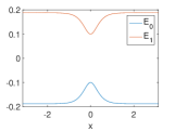
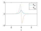
Figure 1: Example 1. Left: Eigenvalues of $M$ (related to the eigenvalues of $H_{e}^{\delta}$ by $F^{\delta}$). Right: the coupling vectors of $H_{e}^{\delta}$, which are invariant with respect to $\delta$ (see text for further discussion).

Example 2. Dual avoided crossing. We choose $H_{e}$ to be

$$H_{e}=\frac{1}{20}\begin{pmatrix}0&0.1e^{-0.06{x^{2}}}\\ 0.1e^{-0.06x^{2}}&-0.5e^{-{x^{2}}}+0.25\end{pmatrix}.$$

Observe that, the two eigenvalues are closest to each other when $x=\pm 1$. The coupling vectors around these points $x=\pm 1$ are significantly larger than their values elsewhere as shown in Figure 2. This explains why the model is often referred to as the dual avoided crossing. The energy surfaces and coupling vector are illustrated in Figure 2.

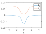
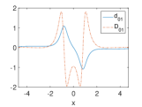
Figure 2: Example 2. Left: Eigenvalues of $H_{e}$. Right: the coupling vectors of $H_{e}$.

Example 3. Extended coupling with reflection. In this example, $H_{e}$ is set to be

$$H_{e}=F\begin{pmatrix}\frac{1}{20}&\frac{1}{20}\left(\arctan(2x)+\frac{\pi}{2}\right)\\ \frac{1}{20}\left(\arctan(2x)+\frac{\pi}{2}\right)&-\frac{1}{20}\end{pmatrix},$$

where

$$F=\frac{1}{20}\left(\arctan(5x)+\frac{\pi}{2}+\delta\right).$$

Hence, as $x\rightarrow\infty$, the eigenvalues of $H_{e}$, $E_{0/1}(x)\rightarrow\mp\pi^{2}/400$, and as $x\rightarrow-\infty$, the eigenvalues of $H_{e}$, $E_{0/1}(x)\rightarrow\mp 0$. As shown in Figure 3, this model involves an extended region of strong nonadiabatic coupling when $x<0$. Moreover, as $x>0$, the upper energy surface is repulsive so that it is likely that trajectories moving from left to right on the excited energy surface will be reflected while those on the ground energy surface will be transmitted. The energy surfaces and coupling vectors are illustrated in Figure 3.

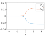
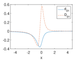
Figure 3: Example 3. Left: Eigenvalues of $H_{e}$. Right: the coupling vectors of $H_{e}$.

Compared to Tully’s extended coupling example in Tully (1990), we slightly modify the potential energy surface so that the eigenvalues $E_{0/1}(x)$ as functions of $x$ become smooth.

IV.2 Convergence test with various $\varepsilon$

In this test, we test the algorithm on Example 1 for $\varepsilon=\frac{1}{32}$, $\frac{1}{64}$ and $\frac{1}{128}$ with $w=2$, $\delta=5\varepsilon$ and $C_{g}=1$. The purpose is to understand the performance of the algorithm for systems with different semiclassical parameter $\varepsilon$. The corresponding energy surfaces are plotted in Figure 4, while the coupling vectors stay unchanged. The initial condition is chosen concentrated on the lower surface only, and assumed to be the Gaussian wave packet

$$u_{0}(0,x)=(32\varepsilon)^{-1/4}e^{\frac{i}{\varepsilon}k_{0}\cdot(x-y_{0})}e^{-\frac{1}{2\varepsilon}(x-y_{0})^{2}},$$ (28)

where $y_{0}$ and $k_{0}$ denote the initial position and momentum of the semiclassical wave packet respectively, the packet is normalzied so that the $L^{2}$ norm is $1$. In the set of tests, we fix $y_{0}=-1.5$ and $k_{0}=1.5$. For the initial trajectory number $M=25$, $50$, $100$, $200$, $400$, $800$, $1600$ and $3200$, the numerical test is repeated for $100$ times in each case, and empirical average of the $L^{2}$ errors of the wave functions with confidence intervals are plotted in Figure 4. We observe that, the numerical error is dominated by the stochastic sampling error which is of order $\mathcal{O}(M^{-1/2})$, which is consistent with the Monte Carlo nature of the algorithm. The stochastic sampling error also appears to be rather independent of the small parameter $\varepsilon$.

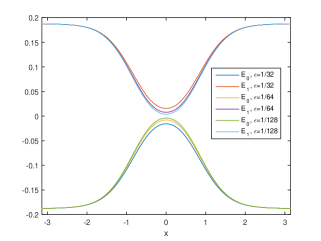
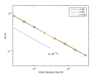
Figure 4: Top: Eigenvalues of $H_{e}$ for $\varepsilon=\frac{1}{32}$, $\frac{1}{64}$ and $\frac{1}{128}$. Bottom: Empirical average of the error in the wave functions with confidence intervals.

IV.3 Error growth in time and conservation of energy in a bouncing back test

We now study the performance of the FGA-SH algorithm in a bouncing back test, to validate the long time accuracy especially when the wave propagation switches direction (bounces back by the energy surface). We choose to focus on Example 1 for the test. We fix $\varepsilon=\frac{1}{32}$, $w=2$, $\delta=\varepsilon$ and $C_{g}=5$. The potential is steeper compared to that of the previous subsection, and therefore the wave packet tends to be bounced back by the steep potential. The initial condition is chosen concentrated on the lower surface only, and takes the same form as (28) with $k_{0}=1.7$ and $y_{0}=-1.5$. We choose these parameters so that the transmitted wave packet will switch direction when propagating on the top energy surface and experience the second significant non-adiabatic transition when it goes through $x=0$ again. We compare the numerical results with initial number of trajectory $M=3200$ to the reference solution till $T=4$. The wave functions obtained by the FGA-SH method with reference solutions are plotted in Figure 5, from which we observe very nice agreement.

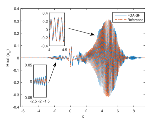
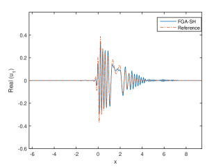
Figure 5: Snapshot of the numerical solutions at $t=4$ (two components of the solution are plotted), note in particular that part of the wave function has bounced back and propagates to the left.

We plot the error in the wave function versus time in Figure 6 (the error is empirically averaged for independent run of $100$ times). It seems that the error grows roughly linearly in time, so the growth is mild. Also, we plot the discrepancy of the total energy between the FGA-SH solutions and the reference solutions. In this test, the initial energy of the wave packet is given by $0.1935$. Besides the averaged error shown in Figure 6, we also note that among the $100$ runs, the largest deviation in energy is $0.0115$. Therefore, the total energy is roughly conserved even in the worst scenario (relative error $5.94\%$). Also, we report the average number of trajectories versus time in Figure 6, which suggests a mild linear growth as the simulation proceeds. This is a good indication that the variance of the algorithm does not grow rapidly in time, while rigorous variance bound is beyond the scope of the current work, and will be leaved for future works.

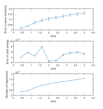
Figure 6: From top to bottom: The error in the wave functions measured in $L^{2}$ metric, the error in total energy, and the number of trajectories as a function of time. The averages and confidence intervals are estimated empirically using $100$ runs.

Let us remark that a major difference between FGA-SH and other FSSH type algorithms is that the trajectory $\widetilde{z}(t)$ is continuous in time on the phase space ${\mathbb{R}}^{2m}$, while in FSSH and other versions of surface hopping, a momentum shift is usually introduced to conserve the classical energy along the trajectory when hopping occurs (if hopping occurs from energy surface $0$ to $1$, it is required that $E_{0}(p,q)=E_{1}(p^{\prime},q)$ where $p^{\prime}$ is the momentum after hopping). Note that as in the FGA for single surface Schrödinger equation, each Gaussian evolved in the FGA-SH does not solve the matrix Schrödinger equation, and only the average of trajectories gives an approximation to the solution. Therefore, it is not necessary for each trajectory to conserve the classical energy. As we have shown, the ensemble average of the trajectories gives good conservation of the energy of the wave packet.

IV.4 Effect of weighting factor $w$

We now numerically demonstrate the role of the weighting factor $\exp(w)$, which is important to get the correct ensemble average of the wave function, since the hopping is driven by a non-homogenous Poisson process (the jumping rate depends on the position and momentum of the trajectory). We choose to focus on Example 1 for the test. We fix $\varepsilon=\frac{1}{32}$, $w=1$, $\delta=\varepsilon$ and $C_{g}=1$. The initial condition is chosen concentrated on the lower surface only, and takes the same form as (28) with $k_{0}=1.5$ and $y_{0}=-1.5$. We run the algorithm with and without the weighting factor $w$ (meaning setting always $w=0$) for $100$ times each, some snapshots of the numerical solutions are plotted in Figure 7, from which we observe that, weighting factors are crucial for accurate approximations of the wave functions.

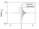
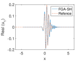
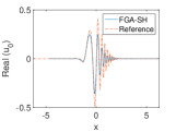
Figure 7: Top: FGA-SH solutions with the weighting factor. Bottom: FGA-SH solutions without the weighting factor.

Also, we summarize the empirical averages and the corresponding variances of the wave functions error and the transition rates (abbreviated by TR) in Table 1. We observe that the weighting factor $w$ is also crucial to get good approximations of the transition rates.

	avg. error	Variance	TR mean	Variance
w/o w.f.	0.2695	9.5780e-03	0.1772	1.0339e-02
with w.f.	0.0678	7.5759e-03	0.2386	1.2106e-02

Table 1: Numerical error in the wave functions, and average transition rates with and without the weighting factor. The reference transition rate is given by $0.2443$; the inclusion of the weighting factor reduces the relative error from $27.5\%$ to $2.33\%$.

IV.5 Initial condition with different momentum

Finally, we test all three examples in Section IV.1 with initial conditions of different momentum, we aim to compare the FGA-SH method with reference solutions in terms of transition rates. We fixed $\varepsilon=\frac{1}{64}$ and initial sample size $M=1600$. The initial condition is chosen concentrated on the lower surface only, and takes the following wave packet form

$$u_{0}(0,x)=(32\varepsilon)^{-1/4}e^{\frac{i}{\varepsilon}K\cdot(x-y_{0})}e^{-\frac{1}{2\varepsilon}(x-y_{0})^{2}},$$

where $y_{0}=-1.5$ and various $K$ are used so that different momentum is considered for the initial wave packet.

For Example 1, we choose $\delta=5\varepsilon$ and test two cases: the small global gap scenario $C_{g}=\frac{1}{20}$ and the large gap scenario $C_{g}=1$. Note that, when $C_{g}=1$, many classically forbidden hops will happen. The FGA-SH algorithm is repeated for $100$ independent trials in each case, and empirical averages of the hopping rates with confidence intervals are plotted in Figure 8, together with the typical number of trajectories at the end of the simulation time. The corresponding results for Example 2 and Example 3 are plotted in Figure 9. We observe that, the FGA-SH results give accurate approximation in the tests. It is also worth pointing out that the error seems to be rather uniform for different values of the initial momentum $K$. We also remark that the birth/death processes adaptively choose the number of trajectories needed, which helps to maintain the uniform accuracy over different initial momentum. From the numerical results, it can be seen that a smaller initial momentum ends up requiring more trajectories.

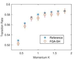
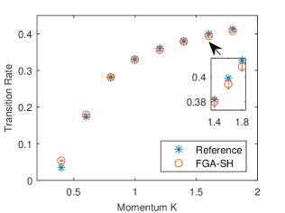
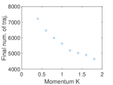
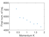
Figure 8: Numerical results of the transition rate of FGA-SH method compared with the reference solution for Example 1. Top: Transition rates for Example 1 with $C_{g}=\frac{1}{20}$ (smaller gap); middle: Transition rates for Example 1 with $C_{g}=1$ (larger gap); bottom left: typical number of trajectories at final time for Example 1 with small $C_{g}$; bottom right: typical number of trajectories at final time for Example 1 with large $C_{g}$.

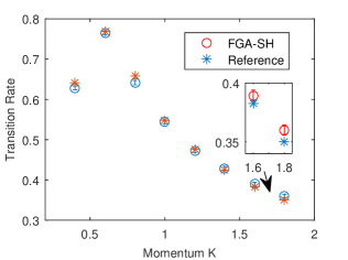
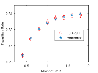
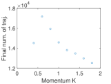
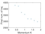
Figure 9: Numerical results of the transition rate of FGA-SH method compared with the reference solution for Example 2 and Example 3. Top: Transition rates for Example 2; middle: Transition rates for Example 3; bottom left: typical number of trajectories at final time for Example 2; bottom right: typical number of trajectories at final time for Example 3.

V Conclusion

In this work we further develop the FGA-SH method, introduced in Lu and Zhou (2016), by proposing an improved sampling algorithm using birth / death branching processes. The algorithm is validated in various numerical tests for the standard test cases for non-adiabatic dynamics.

The path integral interpretation of the fewest switches surface hopping type of algorithm leads to potentially further development for algorithms for non-adiabatic dynamics. Some interesting future directions include validation of the algorithm for higher dimensional problems, non-adiabatic thermal sampling using surface hopping dynamics and also the calculation time-correlation function in the non-adiabatic regime.

Appendix A Asymptotic derivation of the path integral semiclassical approximation

For completeness, we provide a brief explanation of the path integral approximation (6). Please refer to Lu and Zhou (2016) for the detailed asymptotic derivation and mathematical proofs. For simplicity of notation, we assume the initial condition is on the energy surface $E_{0}$, and hence the trajectory starts from that energy surface.

We assume the following deterministic ansatz, referred as surface hopping ansatz, for the solution to (1).

$$u_{\text{FGA}}(T,x)=\lvert 0\rangle\left(u^{(0)}(T,x)+u^{(2)}(T,x)+\cdots\right)\\ +\lvert 1\rangle\left(u^{(1)}(T,x)+u^{(3)}(T,x)+\cdots\right).$$ (29)

This ansatz is similar to that of proposed by Wu and Herman Wu and Herman (2007, 2006, 2005), which is also based on the Herman-Kluk propagators. The two approaches are different however in several essential ways, as elaborated in Lu and Zhou (2016).

The wave function $u^{(n)}$ stands for the contribution with $n$ surface hops before time $t$, starting from surface $E_{0}$. In particular, for trajectories with even number of hops, the electronic state ends at $\lvert 0\rangle$, and trajectories with odd number of hops contribute to $\lvert 1\rangle$. This explains the linear combination in (29). We denote a sequence $\{t_{k}\}_{k=1}^{n}$ for the hopping times satisfying

$$0\leqslant t_{1}\leqslant t_{2}\leqslant\cdots\leqslant t_{n}\leqslant T,$$

at which time the trajectory switches from one energy surface to the other. The ansatz for $u^{(n)}$ is given by

$$u^{(n)}(T,x)=\frac{1}{(2\pi\varepsilon)^{3m/2}}\int\,\mathrm{d}z_{0}\int_{0\leqslant t_{1}\leqslant\cdots\leqslant t_{n}\leqslant T}\\ \tau^{(1)}\cdots\tau^{(n)}\;A^{(n)}\;\exp\left(\frac{i}{\varepsilon}\Theta^{(n)}\right)\,\mathrm{d}T_{n:1},$$ (30)

where $\tau^{(k)}$ is defined in (17) and $\,\mathrm{d}T_{n:1}=\,\mathrm{d}t_{1}\cdots\,\mathrm{d}t_{n}$. Note that in (30), we integrate over all possible hopping times for $n$ hops in the time interval $[0,T]$. Given $\{t_{k}\}_{k=1}^{n}$ and $z_{0}$, the trajectory $\widetilde{z}(t)$ for $0\leqslant t\leqslant T$ is specified.

Substitute the ansatz into the matrix Schrödinger equations and carry out asymptotic calculations as in Lu and Zhou (2016), we arrive at the conclusion that the evolution of $A^{(n)}$ and $\Theta^{(n)}$ should be exactly as that described in Section II.3, such that $u_{\text{FGA}}(T,x)$ is a good approximation to the true solution. Indeed, the asymptotic analysis can be turned into rigorous error analysis Lu and Zhou (2016) that, $u_{\text{FGA}}(T,x)$ is an approximation of the exact solution with $\mathcal{O}(\varepsilon)$ error in $L^{2}$ metric.

Let us now link the deterministic ansatz to the path integral representation. As we discussed in Section II.2, given $T>0$, the number of jumps $n$ of the stochastic trajectory $\widetilde{z}(t)$ for $0\leqslant t\leqslant T$ is a random variable. In particular, by the properties of the associated counting process, the probability that there is no jump $(n=0)$ is given by

$$\mathbb{P}(n=0)=e^{-\int_{0}^{T}\left\lvert\tau^{(1)}\right\rvert\,\mathrm{d}s}.$$ (31)

And, more generally, we have

$$\mathbb{P}(n=k)=\int_{0<t_{1}<\cdots<t_{k}<T}\,\mathrm{d}T_{k:1}\;\prod_{j=1}^{k}\left\lvert\tau^{(j)}\right\rvert\\ \times e^{-\int_{t_{k}}^{t}\left\lvert\tau^{(k+1)}\right\rvert\,\mathrm{d}s}\prod_{j=1}^{k}e^{-\int_{t_{j-1}}^{t_{j}}\left\lvert\tau^{(j)}\right\rvert\,\mathrm{d}s},$$ (32)

and the probability density of $(t_{1},\cdots,t_{k})$ given there are $k$ jumps in total is

$$\varrho_{k}(t_{1},\cdots,t_{k})\propto e^{-\int_{t_{k}}^{t}\left\lvert\tau^{(k+1)}\right\rvert\,\mathrm{d}s}\prod_{j=1}^{k}\left\lvert\tau^{(j)}\right\rvert\times\\ \times\prod_{j=1}^{k}e^{-\int_{t_{j-1}}^{t_{j}}\left\lvert\tau^{(j)}\right\rvert\,\mathrm{d}s},$$ (33)

for $t_{1}\leqslant t_{2}\leqslant\cdots\leqslant t_{n}$, and $0$ otherwise.

Using the above probabilities, we may calculate explicitly the expectation with respect to the trajectory $\widetilde{z}$. We verify that (6) is exactly a stochastic representation of the FGA ansatz given in (29)–(30), where the integrals with respect to $t_{1},\ldots,t_{n}$ are replaced by the averaging of trajectories. In particular, for the functional $\mathcal{F}$ (13), we observe that the term $A(T)\exp\Bigl{(}\frac{i}{\varepsilon}\Theta(T,x)\Bigr{)}$ comes from the integrand in (30). The weight factor $\exp\bigl{(}w(T)\bigr{)}$ comes from the probability of $k$ hops as in (33). The appearance of ratios like $\tau^{(k)}/\lvert\tau^{(k)}\rvert$ in (13) is to match $\tau^{(k)}$ in the integrand (30) with the use of $\lvert\tau^{(k)}\rvert$ in the hopping probability and hence in the expression (33).