Impact of storage competition on energy markets

Abstract

We study how storage, operating as a price maker within a market environment, may be optimally operated over an extended period of time. The optimality criterion may be the maximisation of the profit of the storage itself, where this profit results from the exploitation of the differences in market clearing prices at different times. Alternatively it may be the minimisation of the cost of generation, or the maximisation of consumer surplus or social welfare. In all cases there is calculated for each successive time-step the cost function measuring the total impact of whatever action is taken by the storage. The succession of such cost functions provides the information for the storage to determine how to behave over time, forming the basis of the appropriate optimisation problem. Further, optimal decision making, even over a very long or indefinite time period, usually depends on a knowledge of costs over a relatively short running time horizon—for storage of electrical energy typically of the order of a day or so.

We study particularly competition between multiple stores, where the objective of each store is to maximise its own income given the activities of the remainder. We show that, at the Cournot Nash equilibrium, multiple large stores collectively erode their own abilities to make profits: essentially each store attempts to increase its own profit over time by overcompeting at the expense of the remainder. We quantify this for linear price functions

We give examples throughout based on Great Britain spot-price market data.

1 Introduction

There has been much discussion in recent years on the role of storage in future energy networks. It can be used to buffer the highly variable output of renewable generation such as wind and solar power, and it further has the potential to smooth fluctuations in demand, thereby reducing the need for expensive and carbon-emitting peaking plants. For a discussion of the use of storage in providing multiple buffering and smoothing capabilities, including the ability to integrate renewable generation into energy networks see, for example, the fairly recent review by Denholm et al (2010) [7], and the many references therein. Within an economic framework much of the value of energy storage may be realised by allowing it to operate in a market environment, provided that the latter is structured in such a way as to allow this to happen. Thus the smoothing of variations in demand between, for example, nighttime when demand is low and daytime when demand in high may be achieved by allowing a store to buy energy at night when the low demand typically means that it is relatively cheap, and to sell it again in the day when it is expensive. Similarly, the use of storage for buffering against shortfalls in renewable generation may—at least in part—be effected by allowing storage to operate in a responsive spot-price market when prices will rise at the times of such shortfall. We remark though that if it is intended that the use of storage should facilitate, for example, a reduction in carbon emissions, then there is of course no guarantee that a market environment will in itself permit this to happen; it may be necessary that the market itself, and the rules under which it operates, are correctly structured so as to penalise or prohibit environmentally damaging generation or to reward clean energy production—for some recent insights into the possible unexpected side effects of storage operating in a market, see Virasjoki et al [21].

A small store may be expected to function as a price-taker, buying and selling so as, for example, to maximise its own profit over time. However, a larger store will act as a price-maker, perhaps significantly affecting the market in which it operates, and thus also affecting quantities such as generator costs, consumer surplus and social welfare. Further a number of larger stores, by competing with each other, may smooth prices to the point where they are unable to make sufficient profits as to be economically viable.

Aspects of many of these issues have been explored in the literature. Recent work on the use of storage in a specifically market environment is given by Gast et al [10, 9], Graves et al [11], Hu et al [14] and Secomandi [18]. Sioshansi et at [20] study the effects of storage on producer and consumer surplus and on social welfare. Sioshansi [19] gives an example where storage may may reduce social welfare. Gast et el [9] show how in appropriate circumstances storage may be used to minimise generation costs and thus maximise consumer welfare.

In the present paper we aim to develop a more comprehensive mathematical theory of the way in which storage interacts with the market in which it operates. Our fundamental assumption is that each individual store operates over an extended period of time in such a way as to optimise its “profit”—or equivalently minimise its costs—with respect to time-varying cost functions presented to it. These may represent either the prevailing costs within a free market, as may be natural when the store is independently owned, or adjusted costs which take into account the wider impact of the stores activities, as would be appropriate when the store was owned, for example, by the generators or by society—see Section 5. Thus if it is desirable that a store should function in a particular way—for example, to minimise generation costs—it may be fed the appropriate cost signals and, given those signals, left to perform as an autonomous agent. Such an approach is notably desirable in facilitating distributed control and optimisation within a possibly complex environment. In this paper are particularly interested in studying the economic effects of competition between multiple stores, not least on the viability of the stores themselves. The typically high capital costs of storage, in relation to operating costs, mean that competition between stores may reduce price differentials across time to the extent that stores are unable to make sufficient operating profit as to permit the recovery of their capital costs.

Within our analysis we therefore treat storage as generating its revenue by arbitrage within a market in which prices are low at times of energy surplus and high at times of scarcity. While, within an appropriately structured and responsive market, this may allow storage to operate so as to realise many of its economic benefits, we acknowledge that there are many other uses of storage whose benefits may not be so easily captured. Notably this is the case where storage needs to react on a very short time scale, for example to compensate for sudden shortfalls of generation, or to provide stability within a system, and where there is insufficient time for the value of such actions to be captured within a spot market environment. For some work on the simultaneous use of storage for both arbitrage and buffering against the effects of sudden events see Cruise and Zachary [6], while for work on a whole systems assessment of the value of energy storage see Pudjianto et al [17].

We outline in Section 2 the model for the market in which storage operates. In particular this allows for supply and demand which are sensitive to price, and hence also for an impact on price of the market activities of the storage itself (so that the storage may be considered as a price maker). We assume for the moment (but see also below) that a single store wishes to optimise its own profit, or minimise its own costs, by trading in the market, we formulate the corresponding optimisation problem faced by the store and we state how it may be solved. Formally the environment is deterministic, but we discuss also the extent to which it is possible to proceed similarly in a stochastic environment.

In Section 3 we study the effect of a single profit-maximising store in a market. We look at its effect on both market prices and on consumer surplus and give sensitivity results for the variation of the size of the store. We give examples based on Great Britain market data.

In Section 4 we study a number of competing stores operating in a market. We consider possible models of competition, whereby the stores make bids and clearing prices in the market are determined. We identify Nash equilibria for the model of competition in which stores bid quantities—a generalisation of Cournot competition—give existence and uniqueness results, and show how equilibria may be determined. We further show that, even for this arguably most favourable model of competition (from the point of view of the stores) an oversupply of storage capacity leads to a situation in which, with linear price functions, the total profit made by all the stores is approximately inversely proportional to their number. Essentially what happens here is that, relative to a cooperative solution, each store over-trades in order to acquire a larger share of total profit, thereby impacting on the market in such a way as to reduce price differentials over time and thus also the profits to be made by other stores. Thus a sufficiently large number of stores are unable to make profits, and so—presumably—recoup their capital costs. In this section we also give examples again based on GB market data and relating to such competition between stores.

Finally, in Section 5 we consider variant problems in which storage (instead of consisting of independent profit-maximising entities) is managed, for example, for the optimal benefit of consumers, or for the optimal benefit of generators. We show that, by suitable redefinition of cost functions, these variant problems may be reduced mathematically to those already studied.

2 Model

We now formulate our model for a set of $n\geq 1$ stores operating in an energy market. Formally we treat prices and costs as deterministic. However, in a stochastic environment it may be reasonable, at each successive point in time, to replace future prices and costs by their expected values and to then proceed as in the deterministic case. That this can, in many cases, lead to optimal or near optimal behaviour for a single store is shown in Cruise et al [5]. It is further the case that, for many applications—notably electricity storage—optimal decision making over long or even indefinite time horizons nevertheless only requires a real-time knowledge of future costs over a short running time horizon, something which is again shown formally in [5]. Thus electricity storage may make its profits by exploiting differences between daytime and nighttime prices and if these are sufficiently different that the storage typically fills and empties on a daily—or almost daily basis—then ongoing optimal management may never require a knowledge of future prices for more than a few days ahead.

We assume that each store $j$ has an energy capacity $E_{j}$ and input and output rate constraints $P_{Ij}$ and $P_{Oj}$ respectively (the maximum amount of energy which can enter or leave the store per unit time). Each such store $j$ also has an efficiency $\epsilon_{j}\in(0,1],$ where $\epsilon_{j}$ is the number of units of energy output which the store can achieve for each unit of energy input. We assume without loss of generality that any loss of energy due to inefficiency occurs immediately after leaving the store (so that the above capacity and rate constraints—both input and output—apply to volume of energy input). For simplicity we also assume that there is no time-dependent leakage of energy from the stores; the simple adjustments required to deal with any such leakage are analogous to those described in [5].

We work in discrete time $t=1,\dots,T$ for some finite time horizon $T$. Associated with each such time $t$ is a price function $p_{t}$ such that $p_{t}(x)$ is the market price per unit of energy when $x$ is the total amount (positive or negative) of energy bought from the market by all the stores, i.e. $xp_{t}(x)$ is the total cost to the stores of buying this energy. (Each of the functions $p_{t}$ is of course influenced by everything else that is happening in the market at time $t$; it explicitly measures only the further effect on price of the activity of the stores.) We assume throughout that, over the range of possible values of its argument (i.e. the interval $[-\sum_{j=1}^{n}\epsilon_{j}P_{Oj},\sum_{j=1}^{n}P_{Ij}]$), each of the functions $p_{t}$ is positive and increasing and is such that, for any constant $k$, the function of $x$ given by $xp_{t}(x+k)$ is convex and increasing. (The quantity $xp_{t}(x+k)$ is the total cost to a store of buying $x$ units of energy—again positive or negative—at time $t$ when the total amount bought by the remaining stores at that time is $k$.) An important case in which these conditions are satisfied, and which we consider in detail later, is that where the prices are linearised so that

$$p_{t}(x)=\bar{p}_{t}+p^{\prime}_{t}x$$ (1)

where $\bar{p}_{t}>0$ and where $p^{\prime}_{t}\geq 0$ is such that the function $p_{t}$ remains positive for all possible values of its argument as above. This should, for example, be a good approximation whenever the total storage capacity is not too large in relation to the total size of the market in which the stores operate. In such a case, we may take $\bar{p}_{t}=p_{t}(0)$ (i.e. the price at time $t$ without storage on the system) and $p_{t}^{\prime}=p_{t}^{\prime}(0)$. More generally, the above conditions on the functions $p_{t}$ seem likely to be satisfied in many cases, for example when they do not differ too much from the above linear case, and are in all cases readily checkable.

In particular if $s_{t}(p)$ is the amount externally supplied to the market at time $t$ and price $p$ and $d_{t}(p)$ is the corresponding total demand at that time and price—and if the functions $s_{t}$ and $d_{t}$ are given independently of the activities of any stores—then we may define the residual supply function $R_{t}$ at that time by $R_{t}(p)=s_{t}(p)-d_{t}(p)$; if $R_{t}$ is continuous and strictly increasing then we have that $p_{t}$ is the inverse of the function $R_{t}$ and is similarly continuous and strictly increasing. If, furthermore, each of the functions $R_{t}$ is differentiable and prices take the form (1), with $\bar{p}_{t}=p_{t}(0)$ and $p_{t}^{\prime}=p_{t}^{\prime}(0),$ then we may relate $p_{t}^{\prime}$ to the point elasticities of supply and demand at price $\bar{p}_{t}$, denoted $e_{s}$ and $e_{d}$ respectively, in the following way:

$$p_{t}^{\prime}=\frac{\bar{p}_{t}}{e_{s}s_{t}(\bar{p}_{t})-e_{d}d_{t}(\bar{p}_{t})}.$$ (2)

This method of determining the price functions $p_{t}$ is especially relevant when the other players in the market make their decisions without taking the stores’ actions into account, perhaps due to the relatively small level of storage capacity in relation to the rest of the market. With sufficient information, more complex price functions $p_{t}$ could be derived, for example by considering games between the stores and the rest of the energy system.

We denote the successive levels of each store $j$ by a vector $S_{j}=(S_{j0},\dots,S_{jT})$ where each $S_{jt}$ is the energy level of the store at time $t$. It is convenient to assume that the initial and final levels of the store are constrained to fixed values $S^{*}_{j0}$ and $S^{*}_{jT}$ respectively. For each such vector $S_{j}$ and for each $t=1,\dots,T$, define also $x_{t}(S_{j})=S_{jt}-S_{j,t-1}$ to be the amount (positive or negative) by which the level of the store is increased at time $t$.

In order to incorporate efficiency, it is helpful to define, for each store $j$, the function $h_{j}$ on $\mathbb{R}$ by $h_{j}(x)=x$ for $x\geq 0$ and $h_{j}(x)=\epsilon_{j}x$ for $x<0$. For each time $t$ such that $x_{t}(S_{j})\geq 0$, store $j$ buys $x_{t}(S_{j})$ units of energy from the market, while for $t$ such that $x_{t}(S_{j})<0$, it sells $-\epsilon_{j}x_{t}(S_{j})$ units of energy to the market. For each store $j$ and time $t$, and given the changes $x_{it}$, $j\neq i$, (positive or negative) in the levels of the remaining stores at that time, define now the cost function $C_{jt}(\,\cdot\,;\,x_{it},j\neq i)$ by

$$C_{jt}(x_{jt};\,x_{it},j\neq i)=h_{j}(x_{jt})p_{t}\bigg{(}\sum_{i=1}^{n}h_{i}(x_{it})\bigg{)};$$ (3)

this represents the cost to store $j$ of increasing its level by $x_{jt}$ (again positive or negative) at time $t$, given the corresponding activities of the remaining stores at that time. Note that the conditions on the function $p_{t}$ ensure that $C_{jt}(x_{jt};\,x_{it},j\neq i)$ is an increasing convex function of its principal argument $x_{jt}$ and takes the value zero when this argument is zero.

In particular if the objective of store $j$ is to optimise its profit, given the policy over time $S_{i}=(S_{i0},\dots,S_{iT})$ of every other store $i\neq j$, then it faces the following optimisation problem:

1. $\mathbf{P}_{j}$: Choose $S_{j}=(S_{j0},\dots,S_{jT})$ so as to minimise the function of $S_{j}$ given by

   $$\sum_{t=1}^{T}C_{jt}(x_{t}(S_{j});\,x_{t}(S_{i}),j\neq i)$$ (4)

   subject to the capacity constraints

   $$S_{j0}=S^{*}_{j0},\qquad S_{jT}=S^{*}_{jT},\qquad 0\leq S_{jt}\leq E_{j},\quad 1\leq t\leq T-1.$$ (5)

   and the rate constraints

   $$x_{t}(S_{j})\in X_{j},\qquad 1\leq t\leq T,$$ (6)

   where $X_{j}=\{x:-P_{Oj}\leq x\leq P_{Ij}\}$.

Note that the observed convexity of the cost functions $C_{jt}(\,\cdot\,;\,x_{it},j\neq i)$ ensures that a solution to the optimisation problem $\mathbf{P}_{j}$ always exists.

At various points we make use of the following result, taken from [5], and in which each of the vectors $\mu^{*}_{j}$ is essentially a vector of (cumulative) Lagrange multipliers.

Proposition 1.

For any store $j=1,\dots,n$, and for any fixed policies $S_{i}$ of every other store $i\neq j$, suppose that there exists a vector $\mu_{j}^{*}=(\mu^{*}_{j1},\dots,\mu^{*}_{jT})$ and a value $S_{j}^{*}=(S^{*}_{j0},\dots,S^{*}_{jT})$ of $S_{j}$ such that

1. $S_{j}^{*}$ is feasible for the stated problem $\mathbf{P}_{j}$;

2. for each $t$ with $1\leq t\leq T$, $x_{t}(S_{j}^{*})$ minimises

   $$C_{jt}(x_{jt};\,x_{t}(S_{i}),j\neq i)-\mu^{*}_{jt}x_{jt}$$

   in $x_{jt}\in X_{j}$; and

3. the pair $(S_{j}^{*},\mu_{j}^{*})$ satisfies the complementary slackness conditions, for $1\leq t\leq T-1$,

   $$\begin{cases}\mu^{*}_{j,t+1}=\mu^{*}_{jt}&\quad\text{if $0<S^{*}_{jt}<E_{j}$,}\\ \mu^{*}_{j,t+1}\leq\mu^{*}_{jt}&\quad\text{if $S^{*}_{jt}=0$,}\\ \mu^{*}_{j,t+1}\geq\mu^{*}_{jt}&\quad\text{if $S^{*}_{jt}=E_{j}$.}\end{cases}$$ (7)

Then $S_{j}^{*}$ solves the above optimisation problem $\mathbf{P}_{j}$. Further, the given convexity of the cost functions $C_{jt}(\,\cdot\,;\,x_{t}(S_{i}),j\neq i)$ guarantees the existence of such a pair $(S^{*}_{j},\mu^{*}_{j})$.

In the case of a single store, [5] provides an algorithm which determines a suitable pair $(S_{1}^{*},\mu_{1}^{*})$ satisfying the conditions (i)–(iii) above. A key advantage of the algorithm is its exploitation of the result that the optimal decision of a store at any each successive time $t$ typically depends only on the price information associated with a relatively short interval of time subsequent to $t$. The convexity of the cost functions is required only to guarantee the existence of such a pair, but as long as such a pair exists, the algorithm could be implemented (with some obvious adjustments) to determine the optimal policy of the store under more general cost functions—see Flatley et al [8] for a discussion of this. In Section 4 we adapt the algorithm in [5] to the case of $n$ competing stores.

Remark 1.

In cases where the stores are not independent profit maximising entities but are instead owned by, for example, the generators or by society, the above cost functions $C_{jt}$ may be appropriately modified so that the problems $\mathbf{P}_{j}$ continue to define optimal behaviour for the stores; see Section 5 for a discussion of how this may be done.

3 The single store in a market

In the case $n=1$ of a single store it is convenient to drop the subscript $j$ and to write $S$ for $S_{j}$, etc. The single-store optimisation problem is then to choose $S=(S_{0},\dots,S_{T})$ so as to minimise

$$\sum_{t=1}^{T}C_{t}(x_{t}(S))$$

(where the $C_{t}$ are the cost functions defined by (3)) subject to the capacity constraints (5) and rate constraints (6).

For simplicity we assume the strict convexity of the cost functions $C_{t}$—as, for example, will be the case when the linear approximation (1) holds with $p^{\prime}_{t}>0$ for each $t$. This strict convexity is sufficient to guarantee the uniqueness of the solution $S^{*}$ of the optimisation problem $\mathbf{P}$.

3.1 Sensitivity of store activity to capacity and rate constraints

Let $(S^{*},\mu^{*})$ be the pair identified in Proposition 1, defining the solution $S^{*}$ of the above optimisation problem $\mathbf{P}$. Then the market clearing price at each time $t$ is $p_{t}(h(x_{t}(S^{*}))$. The successive clearing prices then determine such quantities as consumer surplus—in the way we describe later.

As a measure of the sensitivity of the market to variation of the size of the store, we use Proposition 1 to describe briefly how variation of either the capacity or the rate constraints of the store impacts on the solution $S^{*}$ of $\mathbf{P}$. Proposition 1 continues to hold when we allow either the capacity or the rate constraints of the store to depend on the time $t$. Therefore it is sufficient to consider the effect of variation of these constraints at any single time $t_{0}$.

Consider first the effect of an arbitrarily small increase (positive or negative) $\delta E_{t_{0}}$ in the capacity of the store at time $t_{0}$; since the initial and final levels $S_{0}^{*}$ and $S^{*}_{T}$ are fixed we assume $0<t_{0}<T$. It is clear from Proposition 1 that this infinitesimal change has no effect on $S^{*}$ unless $S^{*}_{t_{0}}=E$; further if $\delta E_{t_{0}}>0$ we also require the strict inequality $\mu^{*}_{t_{0}+1}>\mu^{*}_{t_{0}}$. Under these conditions there exist times $t_{1}<t_{0}<t_{2}$, such that the effect of the increment $\delta{}E_{t_{0}}$—provided it is indeed sufficiently small—is to change $\mu^{*}_{t}$, and so also $x_{t}(S^{*})$ (via the condition (ii) of Proposition 1), for $t$ such that $t_{1}<t\leq t_{0}$, both the original and the new values of $\mu^{*}_{t}$ being constant over this interval, and to similarly change $\mu^{*}_{t}$ and $x_{t}(S^{*})$ for $t$ such that $t_{0}<t\leq t_{2}$, again both the original and the new values of $\mu^{*}_{t}$ being constant over this interval; all changes within the second of the above intervals have the opposite sign to those within the first; for all remaining values of $t$, the parameter $\mu^{*}_{t}$ remains unchanged. The change in $\mu^{*}_{t}$ over each of the above intervals is readily determined by the requirement that now $S^{*}_{t_{0}}=E+\delta E_{t_{0}}$. (Thus, for example, for a perfectly efficient store and twice differentiable cost functions $C_{t}$, the effect of an increment $\delta E_{t_{0}}>0$—where $t_{0}$ is such that $\mu^{*}_{t_{0}+1}>\mu^{*}_{t_{0}}$—will be to increase $x_{t}(S^{*})$ in proportion to $1/C_{t}^{\prime\prime}(x_{t}(S^{*}))$ for times $t$ such that $t_{1}<t\leq t_{0}$ and at which the input rate constraint is nonbinding, and to similarly decrease $x_{t}(S^{*})$ in proportion to $1/C_{t}^{\prime\prime}(x_{t}(S^{*}))$ for times $t$ such that $t_{0}<t\leq t_{2}$ and at which the output rate constraint is nonbinding.)

Similarly an arbitrarily small change at time $t_{0}$ in either the input or the output rate constraint has no effect on $(S^{*},\mu^{*})$ unless $\mu^{*}_{t_{0}}$ and $x_{t_{0}}(S^{*})$ are such that that constraint is binding in the solution of the minimisation problem of (ii) of Proposition 1. The effect is then again to change $\mu^{*}_{t}$ and $x_{t}(S^{*})$ for those $t$ in an interval which includes $t_{0}$; both this interval and the required changes are again readily identifiable from that proposition.

3.2 Impact of a store on prices and consumer surplus

Impact on prices.

In general we may expect the impact of the store on the market to be that of smoothing prices over time: the store will in general buy at times when prices are low, thereby competing in the market and increasing prices at those times, and similarly sell at times when prices are high, thereby decreasing them at those times. Relaxing the power rates or capacity constraints of the store may then be expected to result in further smoothing of the prices, as the store is able to buy and sell more at times of low and high prices, thereby augmenting the above effect. We might also expect that increasing the efficiency of the store will further smooth prices, but this is not so clear-cut, as we illustrate in the following example.

Example 1.

Consider price functions of the linear form (1) and a store which operates over just two time steps ($T=2$), starting and finishing empty but not otherwise subject to capacity or rate constraints. Suppose further that $p_{2}=ap_{1}>0$ for some $a>1$. Then, for efficiency $\epsilon$, the store buys $x(\epsilon)$ units of energy at time $1$ and sells $\epsilon x(\epsilon)$ units at time $2$, where

$$x(\epsilon)=\begin{cases}0&\text{if}\quad\epsilon a<1\\ \dfrac{\epsilon p_{2}-p_{1}}{2(p_{1}^{\prime}+\epsilon^{2}p_{2}^{\prime})}&\text{otherwise}.\end{cases}$$ (8)

In the presence of the store the difference between the market clearing price at time $t_{2}$ and that at time $t_{1}$ is given by $p_{2}(\epsilon x(\epsilon))-p_{1}(x(\epsilon))$, and it is easy to check that for suitable values of the parameters $\bar{p}_{t}$, $p^{\prime}_{t}$, $t=1,2$, this expression is an increasing function of $\epsilon$ for $\epsilon$ sufficiently close to $1$—contrary to the expectation mentioned above.

Impact on consumer surplus.

The consumer surplus associated with a demand function $d$ and clearing price $p_{0}$ is usually defined as $\int_{p_{0}}^{\infty}d(p)\,dp$, and so the consumer surplus of the store’s optimal strategy $S^{*}$ is given by

$$\sum_{t=1}^{T}\int_{p_{t}(h(x_{t}(S^{*})))}^{\infty}d_{t}(p)\ dp,$$ (9)

where $d_{t}(p)$ is the consumer demand associated with price $p$ at time $t$. If the size or activity level of the store is such that the price changes caused by its introduction are relatively small, and we additionally make the linear approximation (1), then the change in consumer surplus due to the introduction of the store is well approximated by

$$-\sum_{t=1}^{T}h(x_{t}(S^{*}))p^{\prime}_{t}d_{t}(\bar{p}_{t}).$$ (10)

It might reasonably be expected that, if the store is reasonably efficient ($\epsilon$ is close to one) and if prices are well-correlated with demand, then the store will buy ($x_{t}>0$) at times of low consumer demand and sell ($x_{t}<0$) at times of high consumer demand, and that this will have a beneficial effect on consumer surplus—as suggested by (10) whenever the price sensitivities $p^{\prime}_{t}$ are sufficiently similar to each other. However, these price sensitivities $p_{t}^{\prime}$ do need to be taken into account. Again we give an example.

Example 2.

Consider again a store with linear prices of the form (1), which starts and finishes empty and which operates over just two time steps, i.e. $T=2$. Assume that the power ratings of the store exceed its capacity and that demand is completely inelastic, so that, for $t=1,2,$ there exists $d_{t}^{*}\geq 0$ such that $d_{t}(p)=d_{t}^{*}$ for all prices $p$. Then, from (10), as long as $p_{1}<\epsilon p_{2}$, the change in consumer surplus on introducing the store to the electricity network is

$$\min\left(\frac{\epsilon p_{2}-p_{1}}{2(p_{1}^{\prime}+\epsilon^{2}p_{2}^{\prime})},E\right)\left(\epsilon p_{2}^{\prime}d_{2}^{*}-p_{1}^{\prime}d_{1}^{*}\right),$$

which is clearly negative whenever $\epsilon p_{2}^{\prime}d_{2}^{*}<p_{1}^{\prime}d_{1}^{*}$. In the latter case the price sensitivity $p^{\prime}_{1}$ at time $1$ is sufficiently high that the decrease in consumer surplus at this time as a result the store buying outweighs the increase in consumer surplus at time $2$ as a result of the store selling. Sioshanshi [19] gives similar examples of cases where storage reduces social welfare, defined as a sum of consumer surplus, producer surplus and the store’s profit.

Remark 2.

In the case of linearised prices of the form (1)—so that the cost functions $C_{t}$ are quadratic with a discontinuity of slope at $0$—we can deduce some further results. In particular, both the market clearing price at each time $t$, given by $p_{t}+p^{\prime}_{t}h(x_{t}(S^{*}))$, and the consumer surplus, given by the approximation (10), are then piecewise linear functions of the capacity of the store. This follows from the observations of Section 3.1, in particular from the condition (ii) of Proposition 1, which shows that the vector of optimised levels $S^{*}$ is a piecewise linear function of the vector $\mu^{*}.$ As the capacity $E$ is varied at a single time $t_{0},$ the discussion of Section 3.1 therefore implies that $\mu^{*}$ must vary piecewise linearly with respect to this variation, between the times $t_{1}$ and $t_{2}$ identified above.

3.3 Example

We consider an example based on half-hourly market electricity prices in Great Britain throughout the year 2014. These are the so-called Market Index Prices as supplied by Elexon [1], who are responsible for operating the Balancing and Settlement Code for the Great Britain wholesale electricity market. These are considered to form a good approximation to real-time spot prices.

These prices, given in units of pounds per megawatt-hour, exhibit an approximately cyclical behaviour, being high by day and low by night and, apart from this, are reasonably consistent throughout the year except for some mild seasonal variation, notably that prices are slightly lower during the summer months.

We take the price functions $p_{t}$ to be given by

$$p_{t}(x)=\bar{p}_{t}\left(1+\lambda x\right),$$ (11)

where the $\bar{p}_{t}$, $t=1,\dots T$, are proportional to the spot market prices referred to above. These price functions are a special case of the linear functions (1), in which the price sensitivity $p^{\prime}_{t}$ is proportional to $\bar{p}_{t}$, an assumption which is in many circumstances very plausible; the constant of proportionality $\lambda\geq 0$ may then be considered a market impact factor. The relation (11) also implies that $\lambda$ should be chosen in proportion to the physical size of the unit of energy: for any $k>0$, the substitution of $x/k$ for $x$ and $k\lambda$ for $\lambda$ leaves (11) unchanged. We therefore find it convenient to consider a store whose nominal dimensions are generally held constant, and to allow $\lambda$ to vary: the market impact as $\lambda$ is increased is equivalent to that which occurs when $\lambda$ is held constant and the dimensions of the store are allowed to increase instead. The case $\lambda=0$ corresponds to no market impact (appropriate to a relatively small store). Clearly also there exists $\lambda_{\max}$ such that, for $\lambda\geq\lambda_{\max}$ both the rate and capacity constraints of the store cease to be binding, so that for all $\lambda\geq\lambda_{\max}$ the market impact of the store is the same, and—again by the above scaling argument—may be regarded as that of an unconstrained store.

We take a storage facility with common input and output rate constraints and, without loss of generality, we choose units of energy such that, on the half-hourly timescale of the spot-price data, this common rate constraint is equal to $1$ unit per half-hour. For the numerical example, we in general take the capacity of the store to be given by $E=10$ units; this corresponds to the assumption that the store empties or fills in a total time of $5$ hours. This capacity to rate ratio is fairly typical, being in particular close to that for the Dinorwig pumped storage facility in Snowdonia [2] (though the charge time and discharge times for Dinorwig are approximately 7 hours and 5 hours respectively). We in general take the round-trip efficiency as $\epsilon=0.75$, which is again comparable to that of Dinorwig. Thus the effect on market prices given by varying $\lambda$, which we discuss below, corresponds to that considering the effect on the market of rescaled versions of a facility not too dissimilar from Dinorwig. We also investigate briefly the effect of varying the capacity constraint $E$ relative to the unit rate constraint, and the effect of varying the round-trip efficiency $\epsilon$.

Figure 1 shows, for $E=10$ and $\epsilon=0.75$, the effect of varying the market impact $\lambda$. The control of the store is optimised, as previously discussed, over the entire one-year period for which price data are available (with the store starting and finishing empty). For relatively small values of $\lambda$ the store fills and empties (or nearly so) on a daily cycle, as it takes advantage of low nighttime and high daytime prices. For significantly larger values of the market impact factor $\lambda$, the store no longer fills and empties on a daily basis (as this factor now erodes the day-night price differential as the volume traded increases); however, the level of the store may gradually vary on a much longer time scale as the store remains able to take advantage of even modest seasonal price variations. The first six panels of panels of Figure 1 show plots of the time-varying levels of the store against selected values of $\lambda$. For $\lambda=0$, $\lambda=0.1$ and $\lambda=0.5$ the level of the store is plotted against time for the first two weeks of the year, while for $\lambda=1$, $\lambda=5$ and $\lambda=10$ the level of the store is plotted against time for the entire year. The final panel of Figure 1 shows a plot against time—for the first two weeks of the year—of the market clearing price corresponding to $\lambda=0$, $\lambda=0.5$, and $\lambda=10$. The erosion of the day/night price differential as $\lambda$ increases is clearly seen.

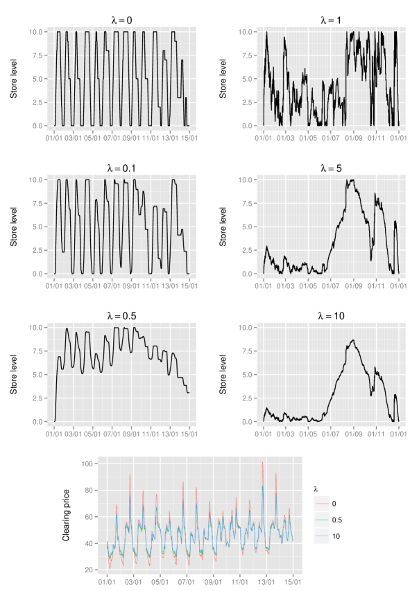
Figure 1: Single store: behaviour of store level and market clearing price (see text for a discussion of units) as the market impact factor $\lambda$ is varied—equivalently the size of the store is varied.

For values of $\lambda$ greater than $\lambda_{\max}\approx 23$ the volumes traded are such that neither the rate nor the capacity constraints of the store are binding, so that for $\lambda>\lambda_{\max}$ volumes traded are simply proportional to $1/\lambda$.

The left panels of Figure 2 show the effect on store level—over the entire year—of decreasing the efficiency of the store from $\epsilon=0.75$ (for which the store level is shown in red) to $\epsilon=0.65$ (for which the store level is shown in blue), for each of the larger values of $\lambda$ considered above, i.e. for $\lambda=1$, $\lambda=5$ and $\lambda=10$. The capacity of the store is here kept at our base level of $E=10$. Decreasing the efficiency of the store reduces its ability to exploit the daily cycle of price variation in a manner not dissimilar from that of increasing the market impact $\lambda$, so that again the volumes of daily trading are reduced, while the store may continue to exploit its full capacity on a seasonal basis—again for a very modest further gain. We remark also that reducing the efficiency of the store reduces the extent to which it is able to smooth prices.

The right panels of Figure 2 similarly show the effect—again over the entire year and for the same three values of $\lambda$—of increasing the capacity of the store from $E=10$ (for which the store level is shown in red) to $E=20$ (for which the store level is shown in blue). The round trip efficiency of the store is kept at $\epsilon=0.75$. In each case it is seen that the daily variation in the level of the store remains much the same as $E$ is increased (since for these levels of $\lambda$ there is too much market impact to make profitable greater volumes of daily trading, except on occasions in the case $\lambda=1$). However, for $\lambda=1$ and for $\lambda=5$, as $E$ is increased the store is able to make some (very modest) additional profit by varying slowly throughout the year the general level at which it operates. For $\lambda=10$ the market impact is so great that the capacity constraint $E=10$—and so also the capacity constraint $E=20$—is never binding, so that in this case the increase in the capacity has no effect.

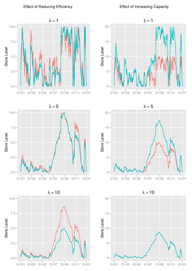
Figure 2: Single store: behaviour of the store level as the round-trip efficiency $\epsilon$ is varied from $0.75$ to $0.65$ (left panels) and as the capacity $E$ is varied from $10$ to $20$ (right panels), in each case for $\lambda=1$, $\lambda=5$ and $\lambda=10$.

4 Competing stores in a market

In this section we discuss $n$ competing stores in a market, where it is assumed that the objective of each store is to maximise its own profit. The optimal strategy of each store in general depends on the activities of the remainder, and what happens depends on the extent to which there is cooperation between the stores. In the absence of any such cooperation we might reasonably expect some form of convergence over time to a Nash equilibrium, in which each store’s strategy is optimal given those of the others. We first discuss briefly the cooperative solution, primarily for the purpose of reference, before considering the effect of market competition.

4.1 The cooperative solution

Here the stores behave cooperatively so as to minimise their combined cost

$$\sum_{i=1}^{n}\sum_{t=1}^{T}h_{i}(x_{t}(S_{i}))p_{t}\bigg{(}\sum_{k=1}^{n}h_{k}(x_{t}(S_{k}))\bigg{)},$$ (12)

subject to the capacity constraints (5) and rate constraints (6). This is a generalisation to higher dimensions of the single-store problem, and we do not discuss a detailed solution here. Note, however, that an iterative approach to the determination of a solution may be possible. Under our assumptions on the price functions, the function of $S_{1},\dots,S_{n}$ given by (12) is convex. For any store $j$, given the levels $S_{i}$ of the remaining stores $i\neq j$, the minimisation of (12) in $S_{j}$ (subject to the above constraints) is an instance of the single-store problem discussed in Section 3—with cost functions modified so as reflect the overall cost to all the stores of the actions of the store $j$. This leads to the obvious iterative algorithm in which (12) is minimised in $S_{j}$ for successive stores $j$ until convergence is achieved. However, the limiting value of $(S_{1},\dots,S_{n})$, while frequently a global minimum, is not guaranteed to be so.

In the case where the stores have identical efficiencies one might also consider the simplified single-store problem in which the individual capacity constraints are summed and individual rate constraints are summed. If the solution to this, suitably divided between the stores (i.e. with a fraction $\kappa_{i}$ of the optimal flow assigned to each store $i$, where $\sum_{i=1}^{n}\kappa_{i}=1$), is feasible for the original problem then it solves that problem. One case where this is true is where additionally the ratios $E_{j}/P_{Ij}$ and $E_{j}/P_{Oj}$ are the same for all stores $j$; the solution to the simplified single-store problem is then just divided among the stores in proportion to their capacities to give the cooperative solution to the $n$-store problem.

The impact of the stores on market prices and consumer surplus is determined in a manner entirely analogous to that of Section 3.2.

4.2 The competitive solution

When stores compete there needs to be a mechanism whereby a clearing price in the market is determined. Here there are in principle various possibilities according to the rules under which the market is to operate. We discuss some of these in Section 4.2.1, making a formal link with the various classical modes of competition in simple “single shot in time” markets for balancing supply and demand in situations where storage does not operate. In the succeeding sections we look in particular at what happens when stores bid quantities, i.e. at Cournot models of competition.

4.2.1 Possible models of competition

Consider first the case $T=2$, and assume for simplicity that the stores are perfectly efficient. Suppose that each store $k$ buys and then sells $q_{k}$ (positive or negative), and that this results in a price differential of $p$ (the clearing price at time 2 less that at time 1) so that each store $k$ makes a profit $pq_{k}$. We might consider the situation where, in a precise analogue of the supply function bidding of Klemperer and Meyer [16], each store $k$ declares, for each possible value of $p$, a value $S_{k}(p)$ which it contracts to buy at time 1 and then sell at time 2 if the clearing prices at those times are set such that the price differential is $p$. If each “supply function” $S_{k}$ is a nondecreasing function of $p$, the auctioneer then chooses the clearing prices $p_{1}$ and $p_{2}$ such that

$$R_{1}(p_{1}) =\sum_{k}S_{k}(p)$$ (13)

$$R_{2}(p_{2}) =-\sum_{k}S_{k}(p)$$ (14)

$$p_{2}-p_{1} =p,$$ (15)

where, for $t=1,2$, $R_{t}$ is the residual supply function defined in Section 2.

Assume that the residual supply functions $R_{t}$ are strictly increasing. The system of equations (13)–(15) is easily seen to have a unique solution (provided the supply functions $S_{k}$ are such that one exists at all): suppose that, as $p$ varies, $p_{1}$ and $p_{2}$ are chosen as functions of $p$ such that $p_{2}-p_{1}=p$ and $R_{2}(p_{2})=-R_{1}(p_{1})$; then, as $p$ increases, $\sum_{k}S_{k}(p)$ increases while $R_{1}(p_{1})$ decreases, and at the unique value of $p$ such that we have equality between these two quantities the above system of equations (13)–(15) is satisfied.

Mathematically, this situation is no different from that of the classical “one-shot” supply function bidding of Klemperer and Meyer [16]. This was further studied in applications to energy markets by Green and Newbery [12] and by Bolle [4], and subsequently by many others—see in particular Anderson and Philpott [3], and the very comprehensive review by Holmberg and Newbery [13]. In such supply function bidding suppliers (for example, electricity generators) submit nondecreasing supply functions to a market in which there is also a nonincreasing demand function, the market clearing price being that at which the total supply equals the total demand. The behaviour of such supply function bidding is considered in [16], in particular the existence and uniqueness of Nash equilibria. In practice one might well wish to restrict the allowable sets of supply functions which suppliers are permitted to bid (see Johari and Tsitsiklis [15]) so as to achieve economically acceptable solutions. Two extreme cases are the classical situations where either suppliers may bid prices at which they are prepared to supply any amount of the commodity to be traded—corresponding to “vertical” supply functions and leading to a Bertrand equilibrium, or else suppliers may bid quantities which they are prepared to supply at whatever price clears the market—corresponding to horizontal supply functions and leading to a Cournot equilibrium. In the former case, at the Nash equilibrium, the one supplier who is able to offer the lowest price corners the market (and, in the case of symmetric suppliers, makes zero profit). In the latter case, modest profits are to be made, but the total profit of all the suppliers decreases rapidly as their number increases—as is seen also in our results for storage models below.

It is difficult to find a sensible and realistic way of extending the concept of general supply function bidding to competition amongst stores operating over more than two time periods—the dimensionality of the space in which the supply functions would then live is too high, and the set of possibilities for market clearing mechanisms is too complex. Nor is it realistic to consider the situation where stores bids prices, since as indicated above, profits are then typically too small for stores to be able to recover their set-up costs. We therefore restrict our attention to the case where stores bid quantities—as seems to be the case where elsewhere in the literature market competition between stores is considered (see, for example, Sioshansi [19]). Here the Nash equilibria are Cournot equilibria and the profits made by the stores at such equilibria may be expected to provide reasonable upper bounds on such profits as might be made in practice—for a review in the context of “one-shot in time” markets again see Holmberg and Newbery [13].

4.2.2 General convex cost functions

We consider stores bidding quantities as above and look for Nash (Cournot) equilibria. A (pure strategy) Nash equilibrium is then a set of vectors $(S_{1},\dots,S_{n})$ such that the strategy $S_{j}$ of each store $j$ (i.e. the vector of quantities traded over time by that store) is optimal given the strategies $S_{i}$, $i\neq j$, of the remaining stores; thus the vector $S_{j}$ solves the optimisation problem $\mathbf{P}_{j}$ (defined by the remaining vectors $S_{i}$, $i\neq j$) of Section 2. Equivalently, at a Nash equilibrium, the vector $S_{j}$ minimises the function (12) subject to the constraints (5) and (6) and with the values of the vectors $S_{i}$, $i\neq j$, held constant.

Broadly what happens at such an equilibrium is that stores will buy and sell more than at the cooperative solution, since each store gains for itself the benefits of so doing, while the corresponding costs are shared out among all stores. In particular consider $n$ identical competing stores with nonbinding capacity and rate constraints, but with common given starting and finishing levels; for the moment assume further that they have round-trip efficiencies $\epsilon=1$, and that the price functions $p_{t}$ are differentiable. For each store $k$ and for each time $t$, write $x_{kt}=x_{t}(S_{k})$. At the symmetric Nash equilibrium, and for each store $j$, there are equalised over time $t$ the partial derivatives with respect to $x_{jt}$ of the functions $x_{jt}p_{t}\bigl{(}\sum_{k=1}^{n}x_{kt}\bigr{)}$. (For $n=1$ these are just the derivatives of the cost functions seen by the store.) It is straightforward to show that the convexity of these functions ensures that in general unit prices received by the store at those times when it is selling are higher than unit prices paid by the store at those times when it is buying, and so the store is able to make a strictly positive profit. However, as $n$ becomes large the above partial derivatives tend to the price functions $p_{t}\bigl{(}\sum_{k=1}^{n}x_{kt}\bigr{)}$ so that, in the limit as $n\to\infty$, prices become equalised over time and the stores no longer make any profit. As earlier, the intuitive explanation is that in the limit the stores become price takers and any individual store is able to exploit any inequality over time in market clearing prices so as to increase its profit. Thus at the Nash equilibrium market clearing prices are equalised over time and stores are unable to make any profit. It is easy to see that essentially the same result holds when round-trip efficiencies are less than one. In the case of linearised price functions we quantify this result further in Theorem 5.

More generally the impact on prices of competition between stores, in comparison to the cooperative solution, is to further reduce the price variation between the different times over which the stores operate. Arguing as in Section 3.2, one would typically expect such increased competition to lead to a further increase in consumer surplus. However, again this need not always be the case.

Existence and uniqueness of Nash equilibria.

The following result shows the existence of a (pure strategy) Nash equilibrium.

Theorem 1.

Under the given assumptions on the price functions $p_{t}$, there exists at least one Nash equilibrium.

Proof.

The assumptions on the price functions $p_{t}$ guarantee convexity of the cost functions defined by (4). We assume first that the price functions are such that these cost functions are strictly convex. Write $S=(S_{1},...,S_{n})$ where each $S_{j}$ is the strategy over time of store $j$. Let $\mathcal{S}$ be the set of all possible $S$; note that $\mathcal{S}$ is convex and compact. Define a function $f:\mathcal{S}\rightarrow\mathcal{S}$ by $f(S)=(f_{1}(S),\dots,f_{n}(S))$ where each $f_{j}(S)$ minimises the function $G_{j}(\,\cdot\,;\,S_{1},\dots,S_{j-1},S_{j+1},\dots,S_{n})$ given by (4) subject to the constraints (5) and (6), i.e. $f_{j}(S)$ is the best response of store $j$ to $(S_{1},\dots,S_{j-1},S_{j+1},\dots,S_{n})$. It follows from the strict convexity assumption that each $f_{j}(S)$ is uniquely defined.

Now suppose that a sequence $(S^{(n)})$ in $\mathcal{S}$ is such that $S^{(n)}\to S$ as $n\to\infty$. Then, for each $j$, the functions $G_{j}(\,\cdot\,;\,S^{(n)}_{1},\dots,S^{(n)}_{j-1},S^{(n)}_{j+1},\dots,S^{(n)}_{n})$ (of $S_{j}$) converge uniformly to the continuous and strictly convex function $G_{j}(\,\cdot\,;\,S_{1},\dots,S_{j-1},S_{j+1},\dots,S_{n})$, so that also $f_{j}(S^{(n)})\rightarrow f_{j}(S)$. Hence the function $f$ is itself continuous. Thus by the Brouwer fixed point theorem there exists $S=f(S)$, which by definition is a (Cournot) Nash equilibrium.

In the case where the price functions $p_{t}$ are such that the cost functions given by (4) are convex but not strictly so, we may consider a sequence of modifications to the former, tending to zero and such that we do have strict convexity of the corresponding cost functions. Compactness ensures that the corresponding Nash equilibria converge, at least in a subsequence, to a limit which straightforward continuity arguments show to be a Nash equilibrium for the problem defined by the unmodified price functions. ∎

In general the uniqueness of any Nash equilibrium is unclear. However, we show in Section 4.2.3 that, under a linear approximation to the price functions, the Nash equilibrium is unique.

The proof of Theorem 1 also suggests an iterative algorithm to identify possible Nash equilibria—analogous to the algorithm suggested in Section 4.1. Given any $S$ the determination of each $f_{j}(S)$ introduced in the above proof requires only the solution of single-store optimisation problem, which may be achieved as described in, for example, [5]). Hence, starting with any $S^{(0)}$, we may construct a sequence $\{S^{(n)}\}_{n\geq 0}$ such that $S^{(n)}=f(S^{(n-1)})$. Then, as in the above proof, any limit $S$ of the sequence $\{S^{(n)}\}$ satisfies $S=f(S)$ and hence constitutes a Nash equilibrium. Different starting points $S^{(0)}$ may be tried, but, in the case of nonuniqueness, there is of course no guarantee that all Nash equilibria will be found.

Even under our given assumptions on the price functions $p_{t}$ the general characterisation of Nash equilibria seems difficult. The following theorem gives a monotonicity result.

Theorem 2.

Consider $n$ competing stores with identical rate constraints and efficiencies and whose starting levels and finishing levels are ordered by their capacity constraints. Then, at any Nash equilibrium $S^{*}=(S^{*}_{1},\dots,S^{*}_{n})$, the levels of the stores are at all times ordered by their capacity constraints.

Proof.

Let $(\mu^{*}_{1},\dots,\mu^{*}_{n})$ be the set of vectors (Lagrange multipliers) associated with the Nash equilibrium $S^{*}=(S^{*}_{1},\dots,S^{*}_{n})$ as defined by Proposition 1. It follows from (ii) of that proposition that, for any $t$, and any $i$, $j$,

$$\mu^{*}_{it}\geq\mu^{*}_{jt}\quad\Longleftrightarrow\quad x_{t}(S^{*}_{i})\geq x_{t}(S^{*}_{j}).$$ (16)

Suppose now that the assertion of the theorem is false. Then there exist $i$, $j$ with $E_{i}<E_{j}$ and some $t_{0}$ such that

$$x_{t_{0}}(S^{*}_{i})>x_{t_{0}}(S^{*}_{j}),\qquad S^{*}_{it_{0}}>S^{*}_{jt_{0}}.$$ (17)

It now follows by induction that, for all $t^{\prime}\geq t_{0}$,

$$x_{t^{\prime}}(S^{*}_{i})\geq x_{t^{\prime}}(S^{*}_{j}),\qquad S^{*}_{it^{\prime}}>S^{*}_{jt^{\prime}},\qquad\mu^{*}_{it^{\prime}}\geq\mu^{*}_{jt^{\prime}}.$$ (18)

That (18) is true for $t^{\prime}=t_{0}$ follows from (16) and (17). Suppose now that (18) is true for some particular $t^{\prime}\geq t_{0}$. It then follows from Proposition 1 that the condition $S^{*}_{it^{\prime}}>S^{*}_{jt^{\prime}}$ implies $\mu^{*}_{i,t^{\prime}+1}\geq\mu^{*}_{j,t^{\prime}+1}$; hence, by (16), $x_{t^{\prime}+1}(S^{*}_{i})\geq x_{t^{\prime}+1}(S^{*}_{j})$ and so finally $S^{*}_{i,t^{\prime}+1}>S^{*}_{j,t^{\prime}+1}$. However, this contradicts the assumption $S^{*}_{iT}\leq S^{*}_{jT}$. ∎

4.2.3 Quadratic cost functions (i.e. linearised price functions)

We can make considerably more progress in the case of the linear approximation to the price functions given by equation (1), where we again assume that, for each $t$, we have $\bar{p}_{t}=p_{t}(0)>0$, $p_{t}^{\prime}=p_{t}^{\prime}(0)\geq 0$, and that the function $p_{t}$ remains positive over the range of possible values of its argument (so that our standing assumptions on the functions $p_{t}$ are satisfied). This linearisation (1) is a reasonable approximation when storage facilities are sufficiently large as to have an impact on market prices, but are not so very large as to require a more sophisticated price function. The main reason for greater analytical tractability in this case is that for a set of vectors $(S_{1},\dots,S_{n})$ to a be Nash equilibrium is then equivalent to the requirement that they minimise a given convex function. In particular we have the following result.

Theorem 3.

Given the price functions (1), there always exists a unique Nash equilibrium.

Proof.

It follows from (1) and (4) that the requirement that a set of vectors $(S_{1},\dots,S_{n})$ be a Nash equilibrium is equivalent to the requirement that, for each store $j$, given the policies $S_{i}$, $i\neq j$, being operated by the remaining stores, the vector $S_{j}$ minimises the total cost

$$\sum_{t=1}^{T}h(x_{t}(S_{j}))\bigg{(}\bar{p}_{t}+p^{\prime}_{t}\sum_{i=1}^{n}h(x_{t}(S_{i}))\bigg{)},$$ (19)

subject to the capacity and rate constraints on store $j$ given by (5) and (6). Now note that this is further equivalent to the requirement that the set of vectors $(S_{1},\dots,S_{n})$ minimises the strictly convex function

$$\sum_{t=1}^{T}\left[\bar{p}_{t}\sum_{i=1}^{n}h_{i}(x_{t}(S_{i}))+\frac{1}{2}p^{\prime}_{t}\left(\sum_{i=1}^{n}h_{i}(x_{t}(S_{i}))^{2}+\bigg{(}\sum_{i=1}^{n}h_{i}(x_{t}(S_{i}))\bigg{)}^{2}\right)\right]$$ (20)

subject to the constraints (5) and (6) being satisfied for all $j$. Further since this minimum is also to be taken over a compact set, its existence and uniqueness—and hence that of the Nash equilibrium—follows. ∎

Theorem 4 below, which is a scaling result, reduces the optimisation problem (the determination of the Nash equilibrium) for $n$ identical competing stores to that of the corresponding problem for an appropriately redimensioned single store.

Theorem 4.

Given the price functions (1) and a common efficiency $\epsilon$, for each $n\geq 1$, consider $n$ identical competing stores with common capacity $E^{(n)}$, common rate input and output constraints $P^{(n)}_{I}$ and $P^{(n)}_{O}$, and common starting and finishing levels $S^{(n)}_{0}$ and $S^{(n)}_{T}$ respectively, where we have

$$E^{(n)}=2E^{(1)}/(n+1),$$

$$P^{(n)}_{I}=2P_{I}^{(1)}/(n+1),\qquad P^{(n)}_{O}=2P_{O}^{(1)}/(n+1),$$

$$S^{(n)}_{0}=2S_{0}^{(1)}/(n+1),\qquad S^{(n)}_{T}=2S_{T}^{(1)}/(n+1).$$

For each $n$, let $S^{(n)}=(S^{(n)}_{1},\dots,S^{(n)}_{T})$ be the common policy over time of each of the stores at the unique and necessarily symmetric competitive Nash equilibrium. Then, at this equilibrium and at each time $t$, the quantity traded by each store in the $n$-store problem is $2/(n+1)$ times the quantity traded in the single store problem, i.e. $h(x_{t}(S^{(n)}))=2h(x_{t}(S^{(1)}))/(n+1)$.

Proof.

It follows from Theorem 3 that, for each $n$, $S^{(n)}$ minimises the strictly convex function

$$n\sum_{t=1}^{T}\left(\bar{p}_{t}h(x_{t}(S^{(n)}))+\frac{1}{2}(n+1)p^{\prime}_{t}h(x_{t}(S^{(n)}))^{2}\right)$$ (21)

subject to the capacity constraints

$$S^{(n)}_{0}=S^{*}_{0}/(n+1),\quad S^{(n)}_{T}=S^{*}_{T}/(n+1),\quad 0\leq S^{(n)}_{t}\leq E/(n+1),\ \,1\leq t\leq T-1,$$

and the rate constraints

$$-P_{I}/(n+1)\leq x_{t}(S^{(n)})\leq P_{O}/(n+1),\quad 1\leq t\leq T.$$

The substitution $z_{t}=2(n+1)x_{t}(S^{(n)})$, for $t=1,\dots,T$, yields a single store minimisation problem which is independent of $n$ (apart from a factor $2n/(n+1)$ in the objective (21)) so that, for each $t$, $x_{t}(S^{(n)})$ (and so also $h(x_{t}(S^{(n)}))$) is proportional to $1/(n+1)$, so that the required result is now immediate. ∎

Remark 3.

The reduction in Theorem 4 (for linear price functions) of the problem for $n$ identical stores to a single store problem, allows also the application of the various sensitivity results of Sections 3.1 and 3.2.

Theorem 5 below shows that $n$ unconstrained stores (with identical efficiencies) in competition make very much less profit in total than a single unconstrained store operating in the same market.

Theorem 5.

Given the price functions (1) and a common efficiency $\epsilon$, consider $n$ stores subject to neither capacity nor rate constraints. Suppose further that the stores have a common starting level $S^{*}_{0}$ and the same common finishing level $S^{*}_{T}=S^{*}_{0}$, and that this level is sufficiently large that, at the (unique and necessarily symmetric) Nash equilibrium, the stores never empty. Then, at this equilibrium, the quantity traded per store is proportional to $1/(n+1)$ and the profit per store is proportional to $1/(n+1)^{2}$.

Proof.

The first assertion of the theorem may be deduced from the scaling result of Theorem 4, and that theorem might be extended to enable also the second assertion of the present theorem to be deduced. However, we use instead the argument below, which also explicitly identifies the behaviour of the stores.

Write $\bar{S}=(\bar{S}_{0},\dots,\bar{S}_{T})$ (where $\bar{S}_{T}=\bar{S}_{0}=S^{*}_{0}$) for the common policy over time of each of the stores at the Nash equilibrium. It now follows from Theorem 3 and the minimisation of the function (20) subject to the constraint

$$\bar{S}_{T}=\bar{S}_{0},$$ (22)

that this equilibrium is given by

$$x_{t}(\bar{S})=\begin{cases}\dfrac{\lambda-\bar{p}_{t}}{(n+1)p^{\prime}_{t}},&\quad\bar{p}_{t}<\lambda\\ 0,&\quad\lambda\leq\bar{p}_{t}\leq\dfrac{\lambda}{\epsilon}\\ \dfrac{\lambda-\epsilon\bar{p}_{t}}{(n+1)\epsilon^{2}p^{\prime}_{t}},&\quad\bar{p}_{t}\geq\dfrac{\lambda}{\epsilon}.\end{cases}$$ (23)

for some Lagrange multiplier $\lambda$ such that (22) is satisfied. Note, in particular, that $\lambda$ is independent of $n$. Thus, as $n$ varies, we have again that $(x_{1}(\bar{S}),\dots,x_{T}(\bar{S}))$ is proportional to $1/(n+1)$ as required. It follows also from (23) (by checking separately each of the three cases there) that, for all $t$,

$$h(x_{t}(\bar{S}))(\bar{p}_{t}+(n+1)p^{\prime}_{t}h(x_{t}(\bar{S})))=\lambda x_{t}(\bar{S}).$$ (24)

It follows from (19) and from (24) that, at the Nash equilibrium, each store $j$ incurs a total cost (the negative of its profit) equal to

$$\sum_{t=1}^{T}h(x_{t}(\bar{S}))(\bar{p}_{t}+np^{\prime}_{t}h(x_{t}(\bar{S}))) =\sum_{t=1}^{T}\lambda x_{t}(\bar{S})-p^{\prime}_{t}h(x_{t}(\bar{S}))^{2}$$

$$=-\sum_{t=1}^{T}p^{\prime}_{t}h(x_{t}(\bar{S}))^{2},$$

where the first equality above follows from (24) and the second from (22). Since, as $n$ varies, $(h(x_{1}(\bar{S})),\dots h(x_{T}(\bar{S})))$ is proportional to $1/(n+1)$, the required result for the profit of each store follows. ∎

Note that, under the conditions of the above theorem, the total quantity traded by the $n$ stores (at each instant in time) is $2n/(n+1)$ times that traded by a single store, while the total profit made by the $n$ stores is $4n/(n+1)^{2}$ times that made by a single store. Thus we here quantify our earlier assertion of the Introduction that competing stores overtrade (for the reasons already discussed there) in comparison to the cooperative solution; as $n\to\infty$ their combined profit decreases towards zero. Clearly also, were the stores subject to capacity or rate constraints, their ability to negatively impact on each other would be less—as in the example below.

4.3 Example

We consider again the half-hourly Market Index Price data for Great Britain throughout 2014, as introduced in the example of Section 3.3. We again let the price function be as given by (11) and (without loss of generality as explained in Section 3.3) take the market impact factor $\lambda=1$. We consider $n=1,2,3$ identical stores in competition, each with a round-trip efficiency $\epsilon=0.75$. For the single-store case $n=1$, we take $E=10$ and common input and output rate constraint $P=1$; for $n=2$ we take $E=5$ and $P=1/2$ for each of the two stores, and for $n=3$ we take $E=10/3$ and $P=1/3$ for each of the three stores. Thus the total storage available in each case is the same. The values of $E$ and $P$ are chosen so that the constraints on the stores are not so severe as to force essentially identical combined behaviour of the stores for each of the three values of $n$ considered; nor are they so lax that the stores behave as if they were unconstrained as considered in Theorem 5. For each $n$, we consider the unique Nash equilibrium in which each of the $n$ stores optimises its behaviour (minimises its cost) over the entire year subject to the constraints of starting and finishing empty, and (for $n>1$) given the behaviour of the remaining store(s).

In the units of the example—for a discussion of which again see Section 3.3—the total profits made throughout the year by the $n$ stores are 4096 for $n=1$, 3733 for $n=2$ and 3267 for $n=3$. For each of the latter two cases, if the stores were to cooperate instead of competing, they would make the same total profit as in the single store case. Thus the decrease in total profit is again due to the effects of competition. However, note that as $n$ increases through the above three values the total profit decreases at a rate which is slower than that in the case of unconstrained stores, as given by Theorem 5.

Figure 3 shows the total level of the $n=1,2,3$ stores and the corresponding market clearing prices (again in the units of the example) over the first two weeks of the year. The upper panel of the figure clearly shows that $n=2$ and $n=3$ competing stores consistently overtrade in relation to the case $n=1$ (corresponding to the cooperative solution). The lower panel shows the extent to which competition between multiple stores smooths market clearing prices, which is of course associated with the reduction in overall profits. The times of maximum store activity correspond to the peaks and troughs of the market clearing price and it is these peaks and troughs which are smoothed by the competition. Note also that, because the round-trip efficiency $\epsilon=0.75$ is significantly less than $1$, there are significant periods of during which the stores neither buy nor sell.

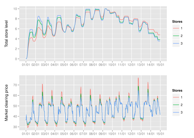
Figure 3: Total store level and market clearing price for each of $n=1,2,3$ stores in competition.

5 Variant problems

Heretofore we have considered the optimal control of stores where the objective of each has in general been to maximise its own profit, obtained through price arbitrage over time. Such behaviour has a variable effect on both producers (in the case of energy the generators) and consumers. However, a store may alternatively be used to maximise the benefit either to the consumers (i.e. to society, if the generators are excluded from the latter), or to the generators, or to society as a whole. We consider briefly each of these possibilities, so as to show that in each case essentially the same mathematical model applies—and hence also both the form of its solution and insights into the effects of competitive behaviour.

One or more stores owned by the consumers.

Suppose that a single store is notionally owned by the consumers (i.e. by society if the latter excludes the generators). Here the problem is to use it so as to maximise the benefit to society. If at each time $t$ an amount $x_{t}$ (positive or negative) is placed in the store, then this has a total consumer cost (again positive or negative) which is the sum of the extra payment to the generator plus the reduction in consumer surplus due to the market impact of the activity of the store (the reduction in consumer surplus being zero in the case where the generator has a flat supply function). The vector $x=(x_{1},\dots,x_{T})$ should then be chosen so as to minimise this total cost, and that is just an instance of the mathematical problem considered in Section 3 and for which Proposition 1 describes the form of the optimal solution. Note that in the case where the generator’s prices are constant over both volume and time, the store, even if perfectly efficient, is of zero value.

One or more stores owned by the generator.

Now suppose that a store is owned by a generator, and is used by the latter with the intention of maximising its own total profit. Thus if, at each time $t$, an amount $x_{t}$ (positive or negative) is placed in the store, then this has a cost to the generator which is simply that of producing it; further, if (at that time) the generator’s production costs are nonlinear, the generator will re-optimise the amount supplied to the market, thereby affecting its profit from that activity; hence we may determine the total cost to the generator of the action $x_{t}$. The vector $x=(x_{1},\dots,x_{T})$ may then be chosen so as to minimise this total cost (i.e. to maximise profit), and this is again just an instance of the problem considered in Section 3. Again in the case where the generator’s production costs are linear and constant over time, the store, even if perfectly efficient, is of zero value.

Both generators and stores owned by society.

Finally suppose that both the generator(s) and any store are owned by the consumers, i.e. by society, and managed jointly so as to maximise the benefit to society. In the absence of the store, the generator’s supply function may be replaced by its (inverse) cost function i.e. that function which gives the amount which may be (just) economically supplied as a (generally increasing) function of unit price; the point of intersection of this function with the demand function gives the optimal price, and the (optimised) benefit to society is the consumer surplus at that price. The introduction of the store now modifies this theory in a manner entirely analogous to that in the earlier case where just the store is owned by society.

6 Conclusions

In the present paper we have considered how storage, operating as a price maker within a market environment, may be optimally operated over an extended or indefinite period of time. The optimality criterion may be that of maximising the profit over time of the storage itself, where this profit results from the ability of the storage to exploit differences in market clearing prices at different times. Alternatively it may be that of minimising over time the cost of generation, or of maximising consumer surplus or social welfare. In all cases there is calculated for each successive step in time the cost function measuring the total impact of whatever action (amount to buy or sell) is taken by the storage. The succession of such cost functions provides the appropriate information to the storage as to how to behave over time, forming the basis of the appropriate mathematical optimisation problem. Further optimal decision making, even over a very long time period, usually depends on a knowledge of costs over a relatively short running time horizon—in the case of the storage of electrical energy typically of the order of a day or so. We have also studied the various economic impacts—on market clearing prices, consumer surplus and social welfare—of the activities of the storage. Where these impacts are considered undesirable, the remedy is again the modification of the successive cost signals supplied to the storage. We have given examples based on real Great Britain market data.

We have be particularly concerned to study competition between multiple stores, where the objective of each store is to maximise its own income given the activities of the remainder. We have shown that at the Nash equilibrium—with respect to Cournot competition—multiple stores of sufficient size collectively erode their own abilities to make profits: essentially each store attempts to increase its own profit over time by overcompeting at the expense of the remainder. We have quantified this in the case of linear price functions, and again given examples based on market data.

References

- [1] https://www.elexon.co.uk/.
- [2] https://en.wikipedia.org/wiki/Dinorwig_Power_Station.
- [3] E. Anderson and A. Philpott. Using supply functions for offering generation into an electricity market. Operations Research, 50(3):477–489, 2002.
- [4] F. Bolle. Supply function equilibria and the danger of tacit collusion. Energy Economics, 14(2):94–102, 1992.
- [5] J.R. Cruise, L.C. Flatley, R.J. Gibbens, and S. Zachary. Optimal control of storage incorporating market impact and with energy applications. http://arxiv.org/abs/1406.3653, 2015.
- [6] J.R. Cruise and S. Zachary. The optimal control of storage for arbitrage and buffering, with energy applications. http://arxiv.org/abs/1509.05788, 2015.
- [7] P. Denholm, E. Ela, B. Kirby, and M.R. Milligan. The role of energy storage with renewable electricity generation. Technical Report NREL/TP-6A2-47187, National Renewable Energy Laboratory, 2010.
- [8] L. Flatley, R.S. MacKay, and M. Waterson. Optimal strategies for operating energy storage in an arbitrage market. http://arxiv.org/abs/1412.0829, 2014.
- [9] N.G. Gast, J-Y. Le Boudec, A. Proutiere, and D.C. Tomozei. Impact of storage on the efficiency and prices in real-time electricity markets. In Proceedings of the fourth international conference on Future energy systems, 2013.
- [10] N.G. Gast, D.C. Tomozei, and J-Y. Le Boudec. Optimal storage policies with wind forecast uncertainties. In Greenmetrics 2012. Imperial College, London, UK, 2012.
- [11] F. Graves, T. Jenkin, and D. Murphy. Opportunities for electricity storage in deregulating markets. The Electricity Journal, 12(8):46–56, 1999.
- [12] R.J. Green and D.M. Newbery. Competition in the british electricity spot market. Journal of Political Economy, 100(25):929–953, 1992.
- [13] P. Holmberg and D. Newbery. The supply function equilibrium and its policy implications for wholesale electricity auctions. Utilities Policy, 18(4):209–226, 2010.
- [14] W. Hu, Z. Chen, and B. Bak-Jensen. Optimal operation strategy of battery energy storage system to real-time electricity price in denmark. In Proc. IEEE Power Energy Soc. Gen. Meet., 2010.
- [15] R. Johari and J.N. Tsitsiklis. Parameterized supply function bidding: Equilibrium and efficiency. Operations Research, 59(5):1079–1089, 2011.
- [16] P.D. Klemperer and M.A. Meyer. Supply function equilibria in oligopoly under uncertainty. Econometrica, 57(6):1243–1277, 1989.
- [17] D. Pudjianto, M. Aunedi, P. Djapic, and G. Strbac. Whole-systems assessment of the value of energy storage in low-carbon electricity systems. IEEE Transactions on Smart Grid, 5:1098–1109, 2014.
- [18] N. Secomandi. Optimal commodity trading with a capacitated storage asset. Management Science, 56(3):449–467, 2010.
- [19] R. Sioshansi. When energy storage reduces social welfare. Energy Economics, 41:106–116, 2014.
- [20] R. Sioshansi, P. Denholm, T. Jenkin, and J. Weiss. Estimating the value of electricity storage in pjm: Arbitrage and some welfare effects. Energy Economics, 31(2):269–277, 2009.
- [21] V. Virasjoki, P. Rocha, A.S. Siddiqui, and A. Salo. Market impacts of energy storage in a transmission-constrained power system. IEEE Transactions on Power Systems, 2015.