Participant number fluctuations for higher moments of a multiplicity distribution

Abstract

The independent participant model is generalized for skewness and kurtosis. The obtained relations allow to calculate the fluctuations of an arbitrarily high order. From the comparison with the SPS and the LHC data it is found that the participants are not nucleons. The contribution of the participant fluctuations increases with the order of fluctuations. The 5% centrality bins selected for the analysis at the LHC by ALICE seems to be too large. The fluctuations measures are dominated by the fluctuations of participants there. The method to quantify the value of participant number fluctuations experimentally is proposed.

Many observables in high energy collisions scale with the number of participants - $N_{\rm P}$ - the nucleons that interacted inelastically during a collision. The total number of charged particles is proportional to $N_{\rm P}$ in the measured energy range Elias:1978ft ; Back:2005hs ; Abbas:2013bpa . This effect was addressed first in Ref. Bialas:1976ed within the wounded nucleon model. It is based on the optical limit of the famous Glauber model Glauber-Notes ; Glauber:2006gd , which physically means that the wounded nucleons emit particles independently from each other. The latter is more general requirement the same as in the independent source model or independent participant model. The term participants is the most commonly used now, therefore it is used later on in this paper.

It was found that the behavior of the scaled variance of a multiplicity distribution as the function of $N_{\rm P}$ can be also qualitatively explained by the fluctuations of participants Konchakovski:2005hq ; Konchakovski:2007zza . The scaled variance is proportional to the second moment of a multiplicity distribution. The ratio of the fourth to the square of the second moment is called kurtosis. The STAR collaboration observes the non-monotonous behavior of the normalized kurtosis for the net-proton distribution Adamczyk:2013dal ; Luo:2015ewa . This might be an indication of the critical point of strongly interacting matter, as higher moments of fluctuations are more sensitive to the proximity of the QCD critical point Stephanov:2008qz . It is quite intriguing that the kurtosis has a minimum in the vicinity of the collision energy where the NA49 and the STAR collaborations see the famous $K^{+}/\pi^{+}$ horn Gazdzicki:1998vd ; Alt:2007aa ; Aggarwal:2010cw ; Das:2014qca . A significant effort of the NA61/SHINE collaboration, the successor of the NA49, is going to be devoted to the study of high order fluctuations. A most challenging background for these studies seems to be the fluctuations of nucleon participants, similar to the case with the scaled variance. These fluctuations are experimentally unavoidable and, therefore, should be reliably estimated. One can derive the necessary formulas for the third moment from the Ref. Olszewski:2015xba , see also Mrowczynski:1999un . However, it seems that, in spite of the practical importance, the influence of the fluctuations of nucleon participants for higher moments was not considered yet.

In the present paper the expressions for the third and the fourth moments are written explicitly for arbitrary distributions of both measured particles and the participants. The only assumptions are that the participants are identical and independent. The proposed method of calculation allows to derive straightforwardly the influence of the participant fluctuations for arbitrarily high moments.

The multiplicity of some particles $N$ created in a collision is the sum of the contributions from $N_{\rm P}$ participants

$$N ~{}=~{}n_{1}~{}+~{}n_{2}~{}+~{}\ldots~{}+~{}n_{{}_{N_{\rm P}}}.$$ (1)

The number of particles $n_{i}$ from a participant $i$ fluctuates. If the participants are identical, then the average $\langle n_{i}\rangle=\langle n_{j}\rangle=\langle n_{1}\rangle$ and

$$\langle N\rangle~{}=\sum_{N_{\rm P}}P(N_{\rm P})~{}\langle~{}\sum_{i=1}^{N_{\rm P}}n_{i}~{}\rangle~{}=\sum_{N_{\rm P}}P(N_{\rm P})~{}N_{\rm P}~{}\langle n_{1}\rangle~{}=~{}\langle N_{\rm P}\rangle~{}\langle n_{1}\rangle~{},$$ (2)

where $P(N_{\rm P})$ is the probability distribution of the participants number. Similarly

$$\langle N^{2}\rangle ~{}=\sum_{N_{\rm P}}P(N_{\rm P})~{}\langle\left(~{}\sum_{i=1}^{N_{\rm P}}n_{i}\right)^{2}\rangle$$

$$~{}=\sum_{N_{\rm P}}P(N_{\rm P})\left(\sum_{i=1}^{N_{\rm P}}\langle n_{i}^{2}\rangle~{}+~{}\sum_{i\neq j=1}^{N_{\rm P}}\langle n_{i}n_{j}\rangle\right)$$

$$~{}=~{}\langle N_{\rm P}\rangle~{}\langle n_{1}^{2}\rangle~{}+~{}\langle N_{\rm P}(N_{\rm P}-1)\rangle~{}\langle n_{1}\rangle^{2}~{},$$ (3)

where the assumption that the participants are independent $\langle n_{i}n_{j}\rangle=\langle n_{i}\rangle\langle n_{j}\rangle=\langle n_{1}\rangle^{2}$ is used. Equations (2) and (Participant number fluctuations for higher moments of a multiplicity distribution) give the famous formula for the scaled variance,

$$\omega~{}=~{}\frac{\langle N^{2}\rangle-\langle N\rangle^{2}}{\langle N\rangle}~{}=~{}\omega_{1}~{}+~{}\langle n_{1}\rangle~{}\omega_{\rm P}~{},$$ (4)

which is present already in Bialas:1976ed . It is the sum of the fluctuations from one participant $\omega_{1}$ and the fluctuations of participant number $\omega_{\rm P}$ times the mean multiplicity of particles of interest from one participant $\langle n_{1}\rangle$. Using the multinomial theorem,

$$\left(n_{1}+n_{2}+\ldots+n_{{}_{N_{\rm P}}}\right)^{k}~{}=~{}\sum_{k_{1},k_{2},\ldots k_{{}_{N_{\rm P}}}}\frac{k!}{k_{1}!k_{2}!\ldots k_{{}_{N_{\rm P}}}!}~{}n_{1}^{k_{1}}n_{2}^{k_{2}}\ldots n_{{}_{N_{\rm P}}}^{k_{{}_{N_{\rm P}}}}~{}\delta\left(k-\sum_{i=1}^{N_{\rm P}}k_{i}\right)~{},$$ (5)

where $\delta$ is the Kronecker delta function, one can obtain arbitrarily high moment in the model of independent participants. For the third and the fourth moments one has:

$$\langle N^{3}\rangle ~{}=~{}~{}\,\,\langle N_{\rm P}\rangle~{}\langle n_{1}^{3}\rangle$$

$$~{}+~{}3\,\langle N_{\rm P}(N_{\rm P}-1)\rangle~{}\langle n_{1}^{2}\rangle\langle n_{1}\rangle$$

$$~{}+~{}~{}\,\,\langle N_{\rm P}(N_{\rm P}-1)(N_{\rm P}-2)\rangle~{}\langle n_{1}\rangle^{3}~{},$$ (6)

$$\langle N^{4}\rangle ~{}=~{}~{}\,\langle N_{\rm P}\rangle~{}\langle n_{1}^{4}\rangle$$

$$~{}+~{}4\,\langle N_{\rm P}(N_{\rm P}-1)\rangle~{}\langle n_{1}^{3}\rangle\langle n_{1}\rangle$$

$$~{}+~{}3\,\langle N_{\rm P}(N_{\rm P}-1)\rangle~{}\langle n_{1}^{2}\rangle^{2}$$

$$~{}+~{}6\,\langle N_{\rm P}(N_{\rm P}-1)(N_{\rm P}-2)\rangle~{}\langle n_{1}^{2}\rangle~{}\langle n_{1}\rangle^{2}$$

$$~{}+~{}~{}\,\,\langle N_{\rm P}(N_{\rm P}-1)(N_{\rm P}-2)(N_{\rm P}-3)\rangle~{}\langle n_{1}\rangle^{4}~{}.$$ (7)

The coefficients in front of the $\langle n_{1}^{k_{i}}\rangle^{k_{j}}$ terms are given by the product of the multinomial coefficient, the number of permutations $\frac{N_{\rm P}!}{(N_{\rm P}-k_{i})!}$, and the additional degeneracy factor that appears due to the fact that the emitted particles are indistinguishable. For example, the factor before $\langle n_{1}\rangle^{4}$ in (7) is equal to the multinomial coefficient $\frac{4!}{1!1!1!1!}=4!$ times the number of ways to pick up four different participants $\frac{N_{\rm P}!}{(N_{\rm P}-4)!}$, divided by the degeneracy factor $4!$ due to the replacement $\langle n_{i}\rangle\langle n_{j}\rangle\langle n_{k}\rangle\langle n_{l}\rangle=\langle n_{1}\rangle^{4}$. The coefficient in front of $\langle n_{1}^{2}\rangle\langle n_{1}\rangle^{2}$ in (7) is equal to $\frac{4!}{2!1!1!0!}=12$ times $\frac{N_{\rm P}!}{(N_{\rm P}-3)!}$, divided by $2!$ due to $\langle n_{i}\rangle\langle n_{j}\rangle=\langle n_{1}\rangle^{2}$, etc.. The sum of all the coefficients for $\langle n_{1}^{k_{i}}\rangle^{k_{j}}=1$ before the averaging over participants gives $N_{\rm P}^{k}$, which can be used for a quick check. The formulas for higher moments can be derived in the similar way. The raw moments $\langle N^{k}\rangle$ are directly related to central moments of a distribution $P(N)$

$$m_{k}~{}=~{}\sum(N-\langle N\rangle)^{k}P(N)~{}.$$ (8)

The second, the third, and the fourth moments in the model of independent participants equal to:

$$m_{2} ~{}=~{}\langle N_{\rm P}\rangle\,m_{2}^{1}~{}+~{}\langle n_{1}\rangle^{2}\,m_{2}^{\rm P}~{},$$ (9)

$$m_{3} ~{}=~{}\langle N_{\rm P}\rangle\,m_{3}^{1}~{}+~{}\langle n_{1}\rangle^{3}\,m_{3}^{\rm P}~{}+~{}3\,\langle n_{1}\rangle\,m_{2}^{\rm P}\,m_{2}^{1}~{},$$ (10)

$$m_{4} ~{}=~{}\langle N_{\rm P}\rangle\,(m_{4}^{1}-3(m_{2}^{1})^{2})~{}+~{}3\,m_{2}^{\rm P}(m_{2}^{1})^{2}~{}+~{}4\,\langle n_{1}\rangle\,m_{2}^{\rm P}\,m_{3}^{1}~{}+~{}6\,\langle n_{1}\rangle^{2}\,m_{3}^{\rm P}\,m_{2}^{1}$$

$$~{}+~{}\langle n_{1}\rangle^{4}\,\left[\,m_{4}^{\rm P}-3(m_{2}^{\rm P})^{2}\,\right]\,+~{}3\,(m_{2})^{2}~{},$$ (11)

where $m_{k}^{1}$ and $m_{k}^{\rm P}$ are defined the same as $m_{k}$ (8) for the distribution of particles produced by one source $P(n_{1})$ and for the distribution of participants $P(N_{\rm P})$.

The combination of central moments gives the scaled variance, the normalized skewness, and the normalized kurtosis:

$$\omega~{}=~{}\frac{m_{2}}{\langle N\rangle}~{}, S\,\sigma~{}=~{}\frac{m_{3}}{m_{2}}~{}, \kappa\,\sigma^{2}~{}=~{}\frac{m_{4}}{m_{2}}~{}-~{}3\,m_{2}~{}, \text{where}~{}~{}\sigma^{2}=m_{2}~{}.$$ (12)

They describe the width, the asymmetry, and the sharpness of a distribution with a single maximum, correspondingly. Skewness and kurtosis are much more sensitive to the properties of a multiplicity distribution. A Poisson distribution has $\omega=S\sigma=\kappa\sigma^{2}=1$ for the same mean multiplicity, while $\omega$ is a free parameter and $S\sigma=\kappa\sigma^{2}=0$ for Normal (Gauss) distribution. In the independent participant model the normalized skewness equals

$$S\,\sigma~{}=~{}\frac{\omega_{1}~{}S_{1}\sigma_{1}~{}+~{}\langle n_{1}\rangle~{}\omega_{\rm P}\left[~{}3\,\omega_{1}~{}+~{}\langle n_{1}\rangle\,S_{\rm P}\,\sigma_{\rm P}~{}\right]}{\omega_{1}~{}+~{}\langle n_{1}\rangle~{}\omega_{\rm P}}~{},$$ (13)

and normalized kurtosis:

$$\kappa\,\sigma^{2}~{}=~{}\frac{\omega_{1}~{}\kappa_{1}\sigma_{1}^{2}~{}+~{}\omega_{\rm P}~{}\left[~{}\langle n_{1}\rangle^{3}~{}\kappa_{\rm P}\,\sigma_{\rm P}^{2}~{}+~{}\langle n_{1}\rangle~{}\omega_{1}\left(~{}3\,\omega_{1}~{}+~{}4\,S_{1}\sigma_{1}~{}+~{}6\,\langle n_{1}\rangle\,S_{\rm P}\,\sigma_{\rm P}~{}\right)~{}\right]}{\omega_{1}~{}+~{}\langle n_{1}\rangle~{}\omega_{\rm P}}~{}.$$ (14)

Scaled variance, skewness and kurtosis depend crucially on the strength of participant fluctuation $\omega_{\rm P}$. If it is zero, then the information about participants is left in the mean multiplicity, but is cancelled in fluctuations:

$$\langle N\rangle~{}=~{}\langle N_{\rm P}\rangle\,\langle n_{1}\rangle~{}, \omega~{}=~{}\omega_{1}~{}, S\,\sigma~{}=~{}S_{1}\,\sigma_{1}~{}, \kappa\,\sigma^{2}~{}=~{}\kappa_{1}\,\sigma_{1}^{2}~{}, \text{for}~{}~{}\omega_{\rm P}~{}=~{}0~{},$$ (15)

so that one observes the fluctuations from one source. It is a desired situation, because participant fluctuations are mainly driven by the uncertainty of the centrality determination. They may mimic or hide the QCD critical point and any other signal. The fluctuations of participants seem to be unavoidable, because one always has a finite centrality window in experiment. If this window is too narrow, then one may cut also the fluctuations from one source. Therefore, one should find the balance between fluctuations of participants $\omega_{\rm P}$, the number and fluctuations of particles from one participant $\omega_{1}/\langle n_{1}\rangle$.

For small fluctuations of the participants, $\omega_{\rm P},\,S_{\rm P}\sigma_{\rm P}\ll\omega_{1}/\langle n_{1}\rangle$ and $\kappa_{\rm P}\sigma_{\rm P}^{2}\ll\omega_{1}^{2}/\langle n_{1}\rangle^{2}$, one obtains:

$$\omega~{}\simeq~{}\omega_{1}~{}, S\,\sigma~{}\simeq~{}S_{1}\,\sigma_{1}~{}+~{}3\,\langle n_{1}\rangle~{}\omega_{\rm P}~{}, \kappa\,\sigma^{2}~{}\simeq~{}\kappa_{1}\,\sigma_{1}^{2}~{}+~{}\langle n_{1}\rangle~{}\omega_{\rm P}\,(3\,\omega_{1}+4\,S_{1}\,\sigma_{1})~{},$$ (16)

i.e., the scaled variance is determined by the fluctuations from one participant, however skewness and kurtosis further depend on how large is the product $\langle n_{1}\rangle~{}\omega_{\rm P}$ compared to the skewness and kurtosis for one source. The fluctuations from one source should be large close to critical point or phase transition. For example, all moments higher than $k>2$ diverge at Bose-Einstein condensation Begun:2016cva , which is the third order phase transition.

For large enough fluctuations of the participants, $\omega_{\rm P}\gg\omega_{1}/\langle n_{1}\rangle$, $\omega_{\rm P}\gg\kappa_{1}\sigma_{1}^{2}/(\langle n_{1}\rangle\,\omega_{1})$, and $S_{\rm P}\sigma_{\rm P}\gg\omega_{1}/\langle n_{1}\rangle$, $S_{\rm P}\sigma_{\rm P}\gg S_{1}\sigma_{1}/\langle n_{1}\rangle$ one finds:

$$\omega~{}\simeq~{}\langle n_{1}\rangle\,\omega_{\rm P}~{}, S\,\sigma~{}\simeq~{}\langle n_{1}\rangle~{}S_{\rm P}\,\sigma_{\rm P}~{}+~{}3\,\omega_{1}~{}, \kappa\,\sigma^{2}~{}\simeq~{}\langle n_{1}\rangle^{2}\,\kappa_{\rm P}\,\sigma_{\rm P}^{2}~{}+~{}6\,\langle n_{1}\rangle\,\omega_{1}\,S_{\rm P}\,\sigma_{\rm P}~{},$$ (17)

i.e., the observed fluctuations are determined mainly by the fluctuations of the participants. Note the $\langle n_{1}\rangle$ and $\langle n_{1}\rangle^{2}$ multipliers in front of scaled variance, skewness and kurtosis from participants in (17). For large energies $\langle n_{1}\rangle$ grows fast and leads to the domination of participant fluctuations for high moments even for relatively small $\omega_{\rm P}$, $S_{\rm P}\,\sigma_{\rm P}$ and $\kappa_{\rm P}\,\sigma_{\rm P}^{2}$. The participant fluctuations are rather large in a standard centrality interval. A finer centrality selection Begun:2006uu or(and) special variables should be used to cancel the fluctuations of participants Gorenstein:2011vq ; Begun:2012wq ; Begun:2014boa .

The experimental information on participant fluctuations is quite ambiguous. The behavior of the scaled variance of a multiplicity distribution in nucleus-nucleus (A+A) collisions as the function of $N_{\rm P}$ was qualitatively explained by the fluctuations of participants both at SPS and at RHIC Konchakovski:2005hq ; Konchakovski:2007zza . However, more recent data of NA49 and NA61/SHINE Lungwitz:2006cx ; Rybczynski-ISMD2013 ; Aduszkiewicz:2015jna show that

$$\omega_{\rm Pb+Pb}^{\rm ch}~{}<~{}\omega_{\rm p+Pb}^{\rm ch}~{}<~{}\omega_{\rm p+p}^{\rm ch}\qquad\text{at SPS}~{},$$ (18)

while one would expect the opposite dependence from the participant model. Using Eq. (4) one obtains

$$\omega_{\rm Pb+Pb}^{\rm ch}~{}=~{}\omega_{1}~{}+~{}\langle n_{\rm Pb+Pb}^{\rm ch}\rangle~{}\omega_{\rm P}~{},\qquad\text{where}~{}~{}\langle n_{\rm Pb+Pb}^{\rm ch}\rangle~{}=~{}\frac{\langle N_{\rm Pb+Pb}^{\rm ch}\rangle}{\langle N_{\rm P}\rangle}~{},$$ (19)

and $\langle n_{\rm Pb+Pb}^{\rm ch}\rangle$ is the number of charged particles per participant. One can see from Eqs. (18) and (19) that the fluctuations in Pb+Pb and p+Pb can not be constructed from fluctuations of p+p. Both $\langle n_{\rm Pb+Pb}^{\rm ch}\rangle$ and $\omega_{\rm P}$ are positive, therefore, if $\omega_{1}=\omega_{\rm p+p}^{\rm ch}$ in (19), then fluctuations of participants, $\omega_{\rm P}$, must be negative in this case. It is impossible, since $\omega$ is positive by definition. However, the fluctuations in p+p and in Pb+Pb are similar at SPS, therefore the relation (18) may be attributed to a combination of some other effects.

The situation should be clear at the LHC, because p+p roughly follow the KNO scaling, which leads to $\omega_{\rm p+p}^{\rm ch}\sim\langle N^{\rm ch}_{\rm p+p}\rangle$ and a fast rise of fluctuations with increasing the energy of the collision, $\sqrt{s_{NN}}$, while for A+A a weaker dependence of fluctuations with energy is expected Heiselberg:2000fk . The ALICE collaboration has published the results for fluctuations of charged particles $\omega^{\rm ch}$ in Pb+Pb collisions within the $|\eta|<0.8$ rapidity range. Their comparison with the AMPT and HIJING string transport models shows different fluctuations and the different dependence on $\langle N_{\rm P}\rangle$ than in the experiment Mukherjee:2016hrj .

Instead of running a transport code one may solve the inverse task. Namely, determine how large should be the fluctuations of the participants in order to describe the data, assuming different fluctuations of the participants. The CMS and the ALICE collaborations have published the data for fluctuations in p+p Khachatryan:2010nk ; Adam:2015gka , as well as the rapidity distributions of charged particles, and the number of participants at different centralities in Pb+Pb at $\sqrt{s_{NN}}=2.76$ TeV Abbas:2013bpa ; Adam:2015kda . Therefore, one can check whether the fluctuations in Pb+Pb is the sum of the fluctuations in p+p and the fluctuations of participants. One should take the measured fluctuations in Pb+Pb, $\omega_{\rm Pb+Pb}^{\rm ch~{}Acc}$, from ALICE Mukherjee:2016hrj . Calculate the rate of how many charged particles are accepted within their rapidity window, $|\eta|<0.8$, with respect to the number of charged particles in the full rapidity $q=\langle N_{\rm Pb+Pb}^{\rm ch}\rangle\big{|}_{|\eta|<0.8}\,/\langle N_{\rm Pb+Pb}^{\rm ch}\rangle$. Then one should use the well known acceptance formula for scaled variance, see e.g. Ref. Begun:2004gs ,

$$\omega^{\rm Acc}~{}=~{}1\,-\,q\,+\,q\,\omega~{},$$ (20)

to reconstruct the fluctuations in the full rapidity range, $\omega=\omega_{\rm Pb+Pb}^{\rm ch}$, then use Eq. (19), and find

$$\omega_{\rm Pb+Pb}^{\rm ch~{}Acc}~{}=~{}1~{}-~{}q~{}+~{}q~{}\omega_{\rm Pb+Pb}^{\rm ch}~{}=~{}\omega_{1}^{\rm Acc}~{}+~{}\langle n_{\rm Pb+Pb}^{\rm ch~{}Acc}\rangle~{}\omega_{\rm P},$$ (21)

where $\omega_{1}^{\rm Acc}=1-q+q\,\omega_{1}$ and $\langle n_{\rm Pb+Pb}^{\rm ch~{}Acc}\rangle=q\,\langle n_{\rm Pb+Pb}^{\rm ch}\rangle$. The fluctuations in p+p equal to $\omega_{\rm p+p}^{\rm Acc}\simeq 4.6,~{}8.46,~{}11.36,~{}13.74$ in the rapidity intervals $|\Delta\eta|=0.5,~{}1.,~{}1.5,~{}2.4$, correspondingly, therefore,

$$\omega_{1}^{\rm Acc}=~{}\omega_{\rm p+p}^{\rm Acc}\big{|}_{|\Delta\eta|<0.8}~{}\simeq~{}7.~{}>~{}\omega_{\rm Pb+Pb}^{\rm ch~{}Acc}~{}\simeq~{}3.~{},$$ (22)

and the fluctuations of the participants are negative in (21), similar to that at the SPS (18). The acceptance $q\simeq 15\%$ in Pb+Pb at ALICE. It gives $\omega_{\rm p+p}=(\omega_{\rm p+p}^{\rm Acc}\big{|}_{|\Delta\eta|<0.8}-1+q)/q\simeq 41$ for the whole acceptance. One may argue that some processes may damp the fluctuations from one participant in Pb+Pb compared to p+p. Let us pick up some numbers in order to quantify a possible outcome and consider three cases.

First, the fluctuations from one source equal to the maximal measured fluctuations in p+p, $\omega_{1}=\omega_{\rm p+p}^{\rm ch}\big{|}_{|\eta|<2.4}=13.74$. Let’s call this case ’Maximal’.

Second, the fluctuations from one source are Poisson-like, $\omega_{1}=\omega_{\rm Poisson}=1$, called ’Poisson’. For these two cases we know all the terms in Eq. (21), except for $\omega_{\rm P}$, which is calculated from (21).

Third case – we do not know the fluctuations from one source, but we know that the fluctuations of participants are of the order of unity, $\omega_{\rm P}=1$, as in HIJING and AMPT in Ref. Mukherjee:2016hrj , and then calculate $\omega_{1}$ from (21). This case is called ’Transport’.

The results are shown in Figs. 1 and 2.

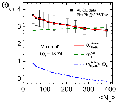
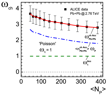
Figure 1: The decomposition of experimentally measured fluctuations of charged particles $\omega_{\rm Pb+Pb}^{\rm ch~{}Acc}$ as the function of the number of participants $\langle N_{\rm P}\rangle$ Mukherjee:2016hrj on the fluctuations due to the fluctuations of participants $\langle n_{\rm Pb+Pb}^{\rm ch~{}Acc}\rangle~{}\omega_{\rm P}$ and due to the fluctuations from one participant $\omega_{1}^{\rm Acc}$ in the measured acceptance, assuming some value of the fluctuations from one participant $\omega_{1}$ in the full acceptance.

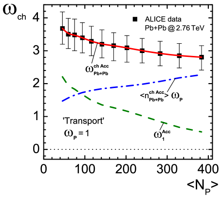
Figure 2: Left: The same as Fig. 1 for the fluctuations of participants $\omega_{\rm P}=1$. Right: The extracted fluctuations of participants, assuming some value of the fluctuations from one source $\omega_{1}$ in the full acceptance.

The continuous lines in Fig. 1 and in Fig. 2 left are the fit of the ALICE data for $\omega_{\rm Pb+Pb}^{\rm ch~{}Acc}$. They go through the data points by definition. The dashed and dash-dotted lines is the decomposition of $\omega_{\rm Pb+Pb}^{\rm ch~{}Acc}$ into two parts according to Eq. (21), right. The corresponding fluctuations of the participants are shown in Fig. 2 right.

The acceptance slowly grows with centrality in the $2.76$ TeV Pb+Pb collisions at the LHC. Therefore, the ’Maximal’ fluctuations from one source, $\omega_{1}^{\rm Acc}$, also grow, while the fluctuations of participants must decrease fast, because the total fluctuations decrease, see Eq. (21). The ’Maximal’ fluctuations from one source are above the experimental measurements for large $\langle N_{\rm P}\rangle$, therefore, the fluctuations of participants, $\omega_{\rm P}$, become negative, which is forbidden by the definition of $\omega$. The absolute value of participant fluctuations is small, so that the measures are done in the ’good’ limit (16). However, $\omega_{\rm P}$ is too small for the LHC, and even smaller than at RHIC, compare the dash-dotted line in Fig. 2 with Fig. 1 from Konchakovski:2007zza .

For ’Poisson’ fluctuations from one source the acceptance dependence is cancelled, $\omega_{1}^{\rm Acc}=\omega_{1}=1$ according to Eq. (20), and the fluctuations of participants are similar to that at RHIC. However, one expects a strong growth of the participant fluctuations with energy from transport models Begun:2012wq . Moreover, the measurements at ALICE are done in the ’bad’ limit, when all the measures are determined by the fluctuations of the participants, see Eq. (17).

The ’Transport’ case is in between the ’Maximal’ and the ’Poisson’, closer to the ’Poisson’. The measurement are done in the ’bad’ limit (17), when the fluctuations of participants determine the results.

One may conclude that the independent participant model can describe fluctuations of charged particles in Pb+Pb at the LHC only if the fluctuations from one participant, $\omega_{1}$, are much smaller than the fluctuations of charged particles in p+p reactions. Therefore, the participants are not nucleons.

If the fluctuations of participants are larger then Poisson, $\omega_{\rm P}\geq 1$, moreover, if they are as large as predicted by transport models, then the 5% centrality bins selected for the analysis at the LHC by ALICE are too large. In this case the fluctuations measures are dominated by the fluctuations of participants and by the corresponding experimental limitations, like the uncertainty in the centrality determination.

There are many ways to look for a possible solution. The participants can be quarks, then the number of particles from one source, $\langle n_{\rm Pb+Pb}^{\rm ch~{}Acc}\rangle$, reduces three times, since there are three quarks in each nucleon. It leads to the increase of the $\omega_{\rm P}$ three times, in order to keep the same value of the product $\langle n_{\rm Pb+Pb}^{\rm ch~{}Acc}\rangle\,\omega_{\rm P}$ in (21). Another possibility is that the sources are not identical and/or strongly correlated. The examination of these possibilities requires further theoretical studies and more data.

One should check experimentally whether participant model works for fluctuation, eliminate the fluctuations of participants, and obtain the fluctuations from one source. In order to do that, one should consider the most central collisions, reduce the centrality window, and check how the fluctuations change, taking, let say, $c=0-20\%$, $c=0-15\%$, $c=0-10\%$, $c=0-5\%$, $c=0-2.5\%$, $c=0-1\%$, etc.. If the participant model works, then one would expect a fast decrease of the fluctuations due to the decrease of the participant fluctuations. The decrease should slow down at some centrality, which is narrow enough, so that the participant fluctuations do not contribute. If the remaining fluctuations are not already Poisson-like due to very small acceptance, then these are the fluctuations from one source.

It seems that the amount of participant fluctuations should be determined before measurements of the higher moments, because participants fluctuations may be strong enough to mimic or hide any other effect.

References

(1)
J. E. Elias et al.,
Phys. Rev. Lett. 41, 285 (1978).
(2)
PHOBOS, B. B. Back et al.,
Phys. Rev. C74, 021901 (2006), nucl-ex/0509034.
(3)
ALICE, E. Abbas et al.,
Phys. Lett. B726, 610 (2013), 1304.0347.
(4)
A. Bialas, M. Bleszynski, and W. Czyz,
Nucl. Phys. B111, 461 (1976).
(5)
R. J. Glauber,
Lectures in theoretical physics, 1959.
(6)
R. J. Glauber,
Nucl. Phys. A774, 3 (2006), nucl-th/0604021.
(7)
V. P. Konchakovski et al.,
Phys. Rev. C73, 034902 (2006), nucl-th/0511083.
(8)
V. P. Konchakovski, M. I. Gorenstein, and E. L. Bratkovskaya,
Phys. Rev. C76, 031901 (2007), 0704.1831.
(9)
STAR, L. Adamczyk et al.,
Phys. Rev. Lett. 112, 032302 (2014), 1309.5681.
(11)
M. A. Stephanov,
Phys. Rev. Lett. 102, 032301 (2009), 0809.3450.
(12)
M. Gazdzicki and M. I. Gorenstein,
Acta Phys. Polon. B30, 2705 (1999), hep-ph/9803462.
(13)
NA49, C. Alt et al.,
Phys. Rev. C77, 024903 (2008), 0710.0118.
(14)
STAR, M. M. Aggarwal et al.,
(2010), 1007.2613.
(15)
STAR, S. Das,
(2014), 1412.0499,
[EPJ Web Conf.90,08007(2015)].
(16)
A. Olszewski and W. Broniowski,
Phys. Rev. C92, 024913 (2015), 1502.05215.
(17)
S. Mrowczynski,
Phys. Lett. B465, 8 (1999), nucl-th/9905021.
(18)
V. Begun,
(2016), 1603.02254.
(19)
V. V. Begun et al.,
Phys. Rev. C76, 024902 (2007), nucl-th/0611075.
(20)
M. I. Gorenstein and M. Gazdzicki,
Phys. Rev. C84, 014904 (2011), 1101.4865.
(21)
V. V. Begun, V. P. Konchakovski, M. I. Gorenstein, and E. Bratkovskaya,
J. Phys. G40, 045109 (2013), 1205.6809.
(22)
V. V. Begun, M. I. Gorenstein, and K. Grebieszkow,
J. Phys. G42, 075101 (2015), 1409.3023.
(23)
NA49, B. Lungwitz et al.,
PoS CFRNC2006, 024 (2006), nucl-ex/0610046.
(24)
M. Rybczynski,
Influence of target on multiparticle production in the forward
domain in p+Pb at 158 GeV,
in Proceedings, 43rd International Symposium on Multiparticle
Dynamics (ISMD 13), 2013.
(25)
NA61/SHINE, A. Aduszkiewicz et al.,
(2015), 1510.00163.
(26)
H. Heiselberg,
Phys. Rept. 351, 161 (2001), nucl-th/0003046.
(27)
ALICE, M. Mukherjee,
Event-by-event multiplicity fluctuations in Pb-Pb collisions in
ALICE,
in 11th Workshop on Particle Correlations and Femtoscopy (WPCF
2015) Warsaw, Poland, November 3-7, 2015, 2016, 1603.06824.
(28)
CMS, V. Khachatryan et al.,
JHEP 01, 079 (2011), 1011.5531.
(29)
ALICE, J. Adam et al.,
(2015), 1509.07541.
(30)
ALICE, J. Adam et al.,
Phys. Lett. B754, 373 (2016), 1509.07299.
(31)
V. V. Begun, M. Gazdzicki, M. I. Gorenstein, and O. S. Zozulya,
Phys. Rev. C70, 034901 (2004), nucl-th/0404056.