Spin dynamics of counterrotating Kitaev spirals via duality

Abstract

Incommensurate spiral order is a common occurrence in frustrated magnetic insulators. Typically, all magnetic moments rotate uniformly, through the same wavevector. However the honeycomb iridates family Li₂IrO₃ shows an incommensurate order where spirals on neighboring sublattices are counter-rotating, giving each moment a different local environment. Theoretically describing its spin dynamics has remained a challenge: the Kitaev interactions proposed to stabilize this state, which arise from strong spin-orbit effects, induce magnon umklapp scattering processes in spin-wave theory. Here we propose an approach via a (Klein) duality transformation into a conventional spiral of a frustrated Heisenberg model, allowing a direct derivation of the dynamical structure factor. We analyze both Kitaev and Dzyaloshinskii-Moriya based models, both of which can stabilize counterrotating spirals, but with different spin dynamics, and we propose experimental tests to identify the origin of counterrotation.

Quantum spin liquid phases Wen (2004) have enjoyed renewed attention in recent years, driven by candidate material platforms. Possible experimental settings in magnetic insulators include the layered kagome systems, the nearly-metallic organics, as well as iridates including the recently explored family of honeycomb iridates, (Na/Li)₂IrO₃ and the related $\alpha$-RuCl₃, distinguished by their significant spin-orbit coupling. Here Ir⁴⁺ (Ru³⁺) hosts an effective $S{=}1/2$, observed to order magnetically at low temperature. While Na₂IrO₃ and $\alpha$-RuCl₃ show collinear zigzag antiferromagnetism Singh and Gegenwart (2010); Liu et al. (2011); Ye et al. (2012); Choi et al. (2012); Singh et al. (2012); Plumb et al. (2014); Sears et al. (2015); Majumder et al. (2015); Johnson et al. (2015); Sandilands et al. (2015, 2016); Banerjee et al. (2016), the three structural polytypes of the lithium iridate, $\alpha$,$\beta$,$\gamma$-Li₂IrO₃, all order into an unconventional incommensurate magnetic phase, involving counterrotating spirals Modic et al. (2014); Takayama et al. (2015); Biffin et al. (2014a, b); Williams et al. (2016).

Recent experiments on $\beta$-Li₂IrO₃ under high pressures Takayama et al. (2015) as well as hydrogenated $\alpha$-Li₂IrO₃ Takayama (2016) under ambient pressure found no evidence for magnetic long-range order at base temperatures, raising the interesting possibility of a transition into a long-sought Kitaev quantum spin liquid. Robustly identifying the properties of such a phase is experimentally rather challenging as the defining long-range entanglement cannot be directly measured in a solid, and the expected emergent fractionalized excitations are predicted to produce only broad spectral features Knolle et al. (2014, 2015); Smith et al. (2016); Nasu et al. (2016); Song et al. (2016); Kimchi et al. (2014). A possible route to quantify proximity to spin-liquid physics is through a knowledge of the appropriate Hamiltonian in the magnetically-ordered phase, whose properties could in principle be more directly accessible experimentally. This requires detailed predictions for characteristic signatures in the spin dynamics for various Hamiltonians to be able to distinguish between competing models.

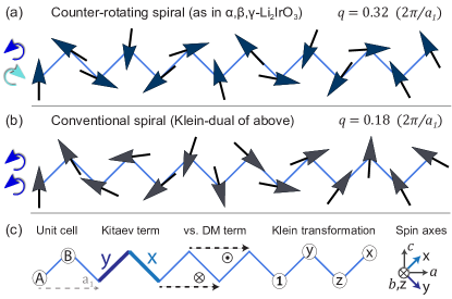
Figure 1: Counterrotating spiral order of $\alpha,\beta,\gamma$-Li₂IrO₃ as the Klein dual of a conventional (co-rotating) spiral.
(a): The counterrotating spiral on a zigzag chain is the unifying common feature of the magnetic structures of all three $\alpha,\beta,\gamma$-Li₂IrO₃ honeycomb iridates. The bottom sublattice rotates clockwise, while the top rotates counterclockwise.
(b): The co-rotating spiral, of a conventional Heisenberg $J_{1}$-$J_{2}$ model, transforms by Klein duality into a counterrotating spiral with a Kitaev-$J_{1}$-$J_{2}$ model and $\mathsf{xy}$ anisotropy.
(c): Competing models to stabilize counterrotation: Kitaev exchange ($\mathsf{x,y}$) or second-neighbor Dzyaloshinskii-Moriya (DM) exchange (out/in for top/bottom bonds). The Klein transformation $\mu\,{\in}\,\{\mathsf{1,x,y,z}\}$ acts as identity $\mathsf{1}$ or by $\pi$ rotation around a spin’s $\mathsf{x,y,z}$ axis. This exact duality for the counterrotating spiral shows its stability and circumvents the magnetic umklapp of its Kitaev exchange for computing its dynamical structure factor.

The counterrotating spiral orders in $\alpha,\beta,\gamma$-Li₂IrO₃ offer a promising avenue for such an approach. However, theoretically computing the spin dynamics has proven to be a nontrivial task. As we show below, the barrier consists of strong magnon umklapp scattering, associated both with the nonuniform spin environment of counterrotation as well as with the lack of any continuous spin rotation symmetry in the Hamiltonian. A similar issue was recently discussed for $\beta$-CaCr₂O₄ Toth and Lake (2015); Damay et al. (2010). Easy-axis and easy-plane anisotropy, as well as antisymmetric Dzyaloshinskii-Moriya (DM) exchange, which are expected to arise from spin-orbit coupling, can preserve a continuous SO(2) symmetry subgroup; in contrast, the “Kitaev” exchange of Kitaev’s honeycomb spin liquid Kitaev (2006), proposed to arise in the honeycomb iridates Jackeli and Khaliullin (2009); Chaloupka et al. (2010); Hwan Chun et al. (2015); Rau et al. (2014); Lee and Kim (2015); Kimchi and Vishwanath (2014), breaks it down to a discrete subgroup. Such a reduced symmetry in a minimal Hamiltonian implies a remarkable spin-orbit coupling effect.

In this work we theoretically analyze the spin dynamics of a minimal 1D model on a zigzag chain with coplanar $\mathsf{xy}$ spiral order with counterrotation on top/bottom sites as shown in Fig. 1(a). This captures the unifying common feature of the magnetic structures in all three Li₂IrO₃ structural polytypes; the actual structures differ in the value of the spin rotation angle, the magnitude of the tilt of the rotation plane away from the $\mathsf{xy}$ plane, and the pattern of those tilts between adjacent chains, and we consider the tilts to be secondary features left for future work. We describe the spin rotation along the zigzag chain via a magnetic ordering wavevector $q$ in units of $2\pi/a_{1}$, where $a_{1}=5.16$ Å is the repeat distance along the zigzag chain, see Fig. 1(c). In this descriptionBiffin et al. (2014a, b); Williams et al. (2016) $q=0.32$ for $\alpha$ and $0.28$ for $\beta$ and $\gamma$-Li₂IrO₃. It is important to note Sup (rial) that while for maximum generality and simplicity we focus here on the parent 1D model, ultimately we want properties that are relevant for 3D systems. Hence we are not interested in the true quantum excitations of an isolated 1D chain Lee et al. (2016), which are usual 1D spinons. Instead, using the spin-wave method we expose precisely those features which are common to the 2D and 3D ordered materials. Our goal is to capture the “semiclassical” quantum fluctuations, appropriate for the real materials, within a unified transparent setting.

The Hamiltonians we study are constructed as the Klein duals of the known parent Hamiltonians for conventional spirals. The Klein duality, a four-sublattice spin transformation whose site-dependent $\pi$ rotations connect to the Kitaev exchange via the multiplication rules of the Klein four group, was previously used to expose a fluctuation-free point in a stripy antiferromagnet Chaloupka et al. (2010) among other contexts Khaliullin and Okamoto (2002, 2003); Khaliullin (2005); Chaloupka et al. (2010, 2013); Kimchi and Vishwanath (2014); Reuther et al. (2012); Li et al. (2015). Here we find that it transforms a co-rotating spiral in a frustrated $J_{1}$-$J_{2}$ model into a counterrotating spiral in a Kitaev-based model, with additional $J_{2}$ $\mathsf{xy}$ anisotropy appropriate for the $\mathsf{xy}$-coplanar spiral mode. We compare this mechanism against a model of antisymmetric DM couplings, here required to be purely intra-sublattice and with a sublattice-dependent orientation Winter et al. (2016). We compute the dynamical spin structure factor for various models of both classes, through a rotating frame exposed by the duality transformation. The dynamics in the Kitaev-based model are found to be quite unusual, but can be interpreted via the duality to the $J_{1}$-$J_{2}$ model’s well-understood dynamics.

The general Hamiltonian consists of the following,

$$H =\sum_{\langle ij\rangle}\left[KS_{i}^{\gamma_{ij}}S_{j}^{\gamma_{ij}}+J_{1}^{\mathsf{xy}}(S_{i}^{\mathsf{x}}S_{j}^{\mathsf{x}}\,{+}\,S_{i}^{\mathsf{y}}S_{j}^{\mathsf{y}})+J_{1}^{\mathsf{z}}S_{i}^{\mathsf{z}}S_{j}^{\mathsf{z}}\right]$$ (1)

$$+\sum_{\langle\langle ij\rangle\rangle}\left[J_{2}^{\mathsf{xy}}(S_{i}^{\mathsf{x}}S_{j}^{\mathsf{x}}{+}S_{i}^{\mathsf{y}}S_{j}^{\mathsf{y}})+J_{2}^{\mathsf{z}}S_{i}^{\mathsf{z}}S_{j}^{\mathsf{z}}\pm D_{2}\,\hat{\mathsf{z}}{\cdot}\vec{S_{i}}{\times}\vec{S_{j}}\right]$$

where $\langle ij\rangle$ and $\langle\langle ij\rangle\rangle$ refer to first and second neighbor bonds, respectively, $\gamma_{ij}\in\{\mathsf{x,y}\}$ is the Kitaev bond type, and the Dzyaloshinskii-Moriya coupling $D_{2}$ is oriented as in Fig. 1c), with $j{>}i$ and $\pm$ sign for the A/B sublattice.

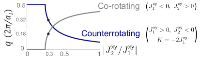
Figure 2: Duality of classical spirals. The classical Heisenberg $J_{1}$-$J_{2}$ model with ferromagnetic $J_{1}<0$ and frustrating second-neighbor $J_{2}>0$ has a (co-rotating) spiral ground state with nonzero wavevector $q$ for $|J_{2}/J_{1}|>0.25$ (gray curve). With easy-plane $\mathsf{xy}$ anisotropy, the resulting $\mathsf{xy}$-plane spiral is independent of $J_{1}^{\mathsf{z}},J_{2}^{\mathsf{z}}$ and depends only on $J_{2}^{\mathsf{xy}}/J_{1}^{\mathsf{xy}}$. The Klein transformation produces a counterrotating spiral with $q\rightarrow\pi/a_{1}-q$ (blue curve) while flipping the signs of $J_{1}^{\mathsf{xy}},J_{2}^{\mathsf{xy}},J_{1}^{\mathsf{z}}$, preserving $J_{2}^{\mathsf{z}}$ and creating a Kitaev exchange $K={-}2J_{1}^{\mathsf{xy}}$. The resulting model has the counterrotating spiral shown in Fig. 1(a) as its classical ground state.

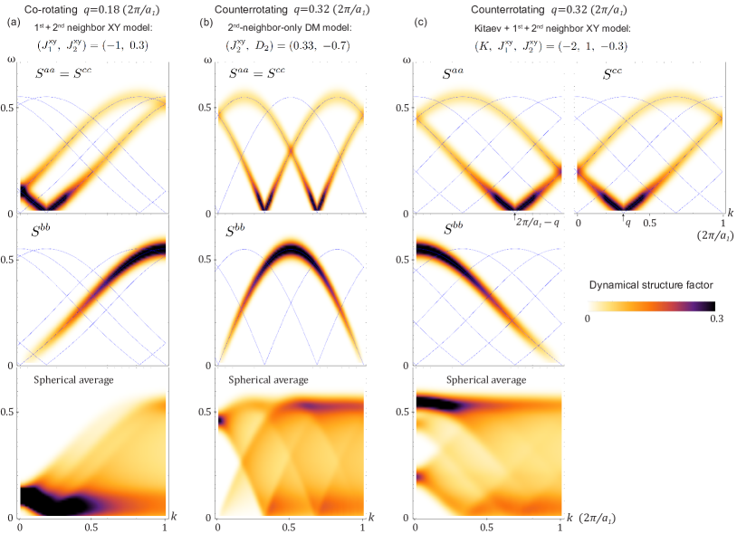
Figure 3: Dynamical structure factor signature of Kitaev exchange. The dynamical correlations of various spin polarizations ($a,b,c$ axes defined in Fig. 1c) are computed via spin wave theory for two possible models of the counterrotating spiral: decoupled sublattices with pure-second-neighbor DM exchanges of opposite signs (column b), and nearest-neighbor Kitaev exchange together with smaller easy-plane $J_{1}$-$J_{2}$ (column c). The plots shown were computed for the minimal models with $J_{1}^{\mathsf{z}},J_{2}^{\mathsf{z}}\rightarrow 0$. (Color is the dynamical spin structure factor, convolved with a $\sigma{=}0.025$ energy Gaussian; thin blue lines are underlying spin wave dispersions.) Magnetic umklapp scattering, which usually breaks down spin waves of the Kitaev exchange, was avoided by tuning to the duality with the conventional co-rotating spiral of a $J_{1}$-$J_{2}$ XY model (panel a). The Klein duality between panels (a) and (c) shifts wavevectors by $\pm\pi/a_{1}$ for $S^{a},S^{c}$ and by $2\pi/a_{1}$ for $S^{b}$, producing distinctive signatures for the Kitaev exchange; for example, the shifted $S^{bb}$ is evident in the spherical average, via the strong signal at high energy and low momentum.

Classical ground states: mechanism for stability of the counterrotating spiral. First let us consider how to stabilize the corotating and counterrotating spirals as ground states for various terms in this Hamiltonian. There are two known mechanisms for stabilizing conventional (corotating) spiral orders: (A) Frustration from competing exchanges, such as ferromagnetic nearest-neighbor and antiferromagnetic second-neighbor exchanges; and (B) DM couplings. As an example of mechanism (A), we take a $J_{1}$-$J_{2}$ ($K=0$) model with $J_{1}<0$ and $J_{2}>0$; its classical ground state is a spiral order with a rotation angle between consecutive sites $\arccos(-J_{1}/4J_{2})$ for $J_{2}>|J_{1}|/4$. For mechanism (B), the rotation angle is $\arctan(D/J_{1})$ for the usual nearest-neighbor DM model. When the zig-zag chain separates into two decoupled A/B chains with DM interaction of opposite sign the angle of rotation for each chain is $\theta_{A,B}=\pm\arctan(D_{2}/J_{2})$.

The Klein duality, which maps a conventional co-rotating spiral to a counterrotating spiral, transforms these conventional spiral Hamiltonians to produce Hamiltonians for the counterrotating spiral. It is easy to see (Fig. 1) how the classical conventional spiral order is transformed, by the rules of the Klein transformation, into the counterrotating spiral order, with $q\rightarrow\pi/a_{1}-q$. Let us then consider how the transformation acts on the Hamiltonians for mechanisms (A) and (B) above, or relatedly on the Hamiltonian Eq. 1 at $K=0$ and uniform orientation of the DM term ($-D_{2}$ rather than $\pm D_{2}$). It is easy to show the following action for the Klein transformation:

$$(J_{1}^{\mathsf{xy}},\ J_{2}^{\mathsf{xy}},\ J_{1}^{\mathsf{z}},\ J_{2}^{\mathsf{z}})\ \leftrightarrow\ (-J_{1}^{\mathsf{xy}},\ -J_{2}^{\mathsf{xy}},\ -J_{1}^{\mathsf{z}},\ +J_{2}^{\mathsf{z}})$$ (2)

$$-D_{2}\ \leftrightarrow\ \pm D_{2}$$ (3)

$$(K=0)\ \leftrightarrow\ (K=-2J_{1}^{\mathsf{xy}})$$ (4)

A Kitaev term is produced, with twice the magnitude and opposite sign relative to the $J_{1}^{\mathsf{xy}}$ term. This transformation is a duality, i.e. it maps Eq. 1 to itself with a different set of parameters.

A known Hamiltonian for a conventional spiral thus produces a Hamiltonian for the counterrotating spiral, via the mapping above. The dual of mechanism (B) is obvious – one can force counter-rotation between sublattices by giving opposite signs to pure-second-neighbor (intra-sublattice) DM terms, as in Eq. 1. The dual of mechanism (A) however produces a Kitaev-based model, with additional first and second neighbor Heisenberg-type terms, whose classical ground state is the counterrotating spiral. We note that the Klein duality necessarily introduces easy-plane anisotropy via the differing transformation of $J_{2}^{\mathsf{z}}$. Since the $J_{1}^{\mathsf{z}},J_{2}^{\mathsf{z}}$ couplings do not change the nature of the spiral order when the spin rotation plane is $\mathsf{xy}$, i.e. for sufficient easy-plane $\mathsf{xy}$ anisotropy, a minimal description is afforded by setting $J_{1}^{\mathsf{z}}{=}J_{2}^{\mathsf{z}}{=}0$. The result (Fig. 2) is a Kitaev-$J_{1}^{\mathsf{xy}}$-$J_{2}^{\mathsf{xy}}$ model whose classical ground state is the counterrotating spiral.

Spin dynamics and magnetic umklapp from spin-orbit coupling. To compute the dynamical structure factor via spin wave theory, one transforms the Hamiltonian Eq. 1 into a “rotating” (or “moving”) frame, i.e. a site-varying coordinate system which is locally aligned with the spin orientation in the ordered spiral configuration. In the following we find it convenient to use the orthorhombic axes $(a,b,c)$ instead of the Kitaev $(\mathsf{x,y,z})$ axes for the spin components, with the relation Kimchi et al. (2015) $\hat{\mathsf{x}}=(\hat{a}+\hat{c})/\sqrt{2}$, $\hat{\mathsf{y}}=(\hat{a}-\hat{c})/\sqrt{2}$ and $\hat{\mathsf{z}}=\hat{b}$ shown in Fig. 1(c), where $\hat{\mathsf{x}}$ indicates a unit vector along $\mathsf{x}$ and so on. Let $R[\theta]$ be a rotation by angle $\theta$ around the spin $\mathsf{z}\equiv b$ axis. The local spin orientation in the wavevector-$q$ spiral is expressed by $e^{3}\equiv R[{-}\eta_{s}qr]\cdot\hat{c}$. Here the sublattice sign $\eta_{s}$ is $\eta_{s}=\mp$ on the A/B sublattice for the counterrotating spiral, or is uniformly $\eta_{s}=+$ for the co-rotating spiral. The local coordinate system $e^{\pm}\equiv R[{-}\eta_{s}qr]\cdot(\hat{a}\pm i\hat{b})$ can then be used to write the spin operator as $\vec{S}=e^{3}S^{3}+(e^{-}S^{+}+e^{+}S^{-})/2$. In the $1/S$ spin wave expansion, $S^{3}\rightarrow 1/2-b^{\dagger}b$ and $S^{\pm}\rightarrow b,b^{\dagger}\equiv a^{\pm}$. The spin wave Hamiltonian is then $H_{\text{SW}}=\sum_{ij}\left[\tilde{J}_{i,j}^{\mu\rho}\,\sigma^{1}_{\rho\nu}/8-\delta_{\mu\nu}\delta_{ij}E_{\text{cl}}/2\right]\left(a^{\mu}_{i}\right)^{\dagger}a^{\nu}_{j}$ with repeated indices summed. The important ingredient is the interaction matrix in the rotating frame, $\tilde{J}_{i,j}^{\mu,\nu}\equiv e^{\mu}_{i}{\cdot}J_{i,j}{\cdot}e^{\nu}_{j}$, where $J_{i,j}$ is the spin interaction matrix between spins $i,j$ associated with Eq. 1.

We thus turn to evaluate the interactions in the rotating frame, $\tilde{J}_{i,j}^{\mu\nu}$. The rotation around $\mathsf{z}\equiv b$ leaves $\hat{b}$ invariant, $e^{\pm}=(R\cdot\hat{a})\pm i\hat{b}$, so its effects are contained in the $R\cdot\hat{a}$ component; for concreteness, we can isolate it by setting $J_{1}^{\mathsf{z}}=J_{2}^{\mathsf{z}}=0$, in which case $\tilde{J}\rightarrow\hat{a}\cdot R^{T}\cdot J\cdot R\cdot\hat{a}$. Evaluating this term on nearest-neighbor bonds $(i,j)$, which connect opposite sublattices, we findSup (rial)

$$\tilde{J}_{i,j} =\hat{a}\cdot R^{T}[-\eta_{s}qr]\cdot J_{i,j}\cdot R[\eta_{s}q(r+a_{1}/2)]\cdot\hat{a}$$ (5)

$$=-\frac{K}{2}\sin\left(\frac{qa_{1}}{2}\right)+\left[J_{1}^{\mathsf{xy}}+\frac{K}{2}\right]\cos\left(\frac{qa_{1}}{2}+2qr\right)$$

where $\eta_{s}=\mp$ is defined by the A/B sublattice of site $i$, at position $r$. The explicit dependence on coordinate $r$ in the last term — the rotated Hamiltonian is not translationally invariant — changes the spin wave physics drastically. This is exposed by Fourier transform, where the expression above produces magnetic umklapp terms such as $b^{\dagger}_{k}b_{k+2q}$. The magnons experience magnetic umklapp scattering that changes their wavevector by multiples of $q$. Even if $q$ is taken to be approximately commensurate, the wavevector quantum number $k$ is lost outside of a highly-folded magnetic Brillouin zone; for incommensurate $q$, the magnon wavevector $k$ becomes ill-defined.

One might generally expect to lose the wavevector quantum number $k$ when translation symmetry is fully broken by an incommensurate order; this is masked in conventional spirals through a rotating frame, which relies on continuous SO(2) rotation symmetry in the model Hamiltonian. The SO(2)-symmetric $J_{2}^{\mathsf{xy}}$-$D_{2}$ second-neighbor model of the counterrotating spiral can similarly preserve the magnon wavevector $k$. However the counterrotation configuration means that each spin has a different local (nearest-neighbor) environment, giving rise to magnetic umklapp processes even through the SO(2)-symmetric $J_{1}^{\mathsf{xy}}$ term, as well as through the discrete-symmetry $K$ terms. The loss of $k$ as a good quantum number is fully apparent.

Here we circumvent the magnetic umklapp scattering by tuning parameters to the duality with the co-rotating spiral. Recall from Eq. 4 that the counterrotating spiral Hamiltonian with $K=-2J_{1}^{\mathsf{xy}}$ is dual to a $J_{1}$-$J_{2}$ XY model. The continuous SO(2) symmetry group of the XY model is preserved in an altered form by the duality, allowing the Hamiltonian at $K=-2J_{1}^{\mathsf{xy}}$ to preserve the magnon quantum numbers. Indeed, Eq. 5 shows that the translation symmetry in the rotated frame is restored when $K+2J_{1}^{\mathsf{xy}}=0$. We proceed by analyzing this case. Perturbations away from this parameter point will generically open gaps in the spin wave dispersions via Bragg reflections through multiples of the spiral wavevector $q$, such as at wavevectors $k=\pm q$, as well as mix the $S^{a}$, $S^{c}$ spin polarizations.

Using the counterrotating spiral model produced by the duality, the dynamical structure factor can be computed straightforwardly by diagonalizing the spin wave Hamiltonian. The results are shown in Fig. 3, for various polarizations as well as for a spherical average relevant to powder samples. The Kitaev-based model shows unusual features, which are nevertheless transparently related, via the Klein duality, to the usual features from the conventional spiral. The duality shifts magnon wavevectors by $\pm\pi/a_{1}$ for the $S^{a}$ and $S^{c}$ spin components, respectively, and by $2\pi/a_{1}$ (corresponding to Néel correlations) for the $S^{b}$ spin component. The Bragg peaks and intensity pattern are thus found by appropriately shifting the known structure factor of the $J_{1}$-$J_{2}$ conventional spiral. Observe that the counterrotating spiral can be considered as a sum of two distinct $S^{a}$, $S^{c}$ spin density waves $\pi/2$ out-of-phase. The two sublattices have in-phase $S^{c}$ but $\pi$-out-of-phase ($2\pi/a_{1}$-modulated) $S^{a}$, producing $S^{c}$-polarized Bragg peaks at $k=0\pm q$, but $S^{a}$-polarized Bragg peaks at $k=2\pi/a_{1}\pm q$. Universal, linearly-dispersing Goldstone modes with the same polarization as the Bragg peaks emerge from $q$ and $2\pi/a_{1}\pm q$ positions. The $S^{bb}$ dynamical correlations (out-of-plane fluctuations) contain a mode with maximum energy and strong intensity at the zone center ($k=0$), as in other Kitaev-based models Chaloupka et al. (2013). We expect these generic features survive when the 1D chains are coupled together Kimchi et al. (2015) as in the actual 2D and 3D honeycomb iridates and to help distinguish between Kitaev or other exchange models.

Conclusion. We have identified a transparent theoretical mechanism for the key feature in the unconventional magnetic orders recently observed in three honeycomb iridates. These materials host different crystal structures but nonetheless their magnetism shares the unifying feature of counterrotating spirals, with opposite handedness in neighboring sublattices. This magnetic configuration, as well as a Kitaev-based parent Hamiltonian, are constructed by acting with the Klein duality on the well-understood frustrated $J_{1}$-$J_{2}$ model of a spiral order. This connection also enables us to solve for the spin dynamics in this system, and to interpret them transparently. We have identified key features in the dynamical structure factor, that could be tested via polarized and unpolarized inelastic neutron scattering or resonant inelastic x-ray scattering experiments. Our work helps build towards a full understanding of the lattice-scale model Hamiltonians for these systems, which would shed further light on the unusually similar features across these disparate materials, as well as enable a controlled identification and understanding of possible proximity to a spin liquid state.

Acknowledgements. We thank Ashvin Vishwanath, Lucile Savary, Samuel Lederer, Jonathan Ruhman, and Yong-Baek Kim for related discussions. I.K. was supported by the MIT Pappalardo postdoctoral fellowship. R.C. acknowledges support from EPSRC (U.K.) through Grant No. EP/H014934/1.

Supplementary Material

The Supplementary Material is divided into five sections. Section (1) shows additional plots of the structure factor. Section (2) gives a short note on the 1D and spin wave approximations. Section (3) gives further detail on the duality between conventional co-rotating and the unconventional counterrotating spirals. Section (4) gives further detail on the spin interactions in the spiral rotating frame, and the spin wave Hamiltonian. Section (5) gives further detail on the computations of the dynamical spin structure factors.

.1 Supplementary Material: (1) Additional plots

See Figs. 4 and  5 for plots of the structure factor for two additional models: (A) a Kitaev-based model with nonzero values of ${\mathsf{z}}$-axis couplings, away from the XY limit, in Fig. 4; and (B) a second neighbor DM model perturbed by adding small inter-sublattice couplings, in Figs. 5. The results for these models and for various other intermediate parameters maintain the features described in the main text.

.2 Supplementary Material: (2) A note on quantum vs. classical approximations in the 1D minimal model

We note that while for maximum generality and simplicity we focus here on a 1D model, ultimately we want properties that are relevant for 3D systems. Hence we are not interested in the true quantum excitation spectrum of an isolated 1D chain, as would be accessible within e.g. DMRG. Such a spectrum would contain the usual 1D spinon excitations, which do not generalize to 2D and 3D magnetic systems. For example, the quantum ground state of the XXZ $J_{1}$-$J_{2}$ model is known, and has short ranged spiral order instead of a long range spiral state, as is necessary due to the Mermin-Wagner theorem in 1D since the incommensurate spiral breaks a continuous symmetry. By treating the 1D minimal model within a spin-wave approximation, we avoid any purely-1D effects, such as spin-charge separation (which here would be manifested as spurious 1D deconfined spinons) and Mermin-Wagner destruction of long range order, which are not relevant for the actual materials. Since our 1D system serves as a minimal model for full 3D systems, which are known to exhibit long range ordering, the appropriate minimal 1D model — that captures the essential low-energy physics of the 3D quantum model relevant for the real materials — is the 1D classical, rather than quantum, model, together with its semiclassical spin wave spectrum.

It is also worth noting a sublety in applying spin-wave theory to materials which, though exhibiting an ordered ground state, are thought to be proximate to a quantum spin liquid. Proximity to a spin liquid cannot be established in the 3D quantum phase diagrams, but a pure-Kitaev Hamiltonian is exactly solvable and exhibits a spin liquid ground state in both 2D and 3D. A model where the Kitaev exchange is significantly larger than any other exchange is then, in some loosely defined sense, potentially proximate to the large-Kitaev quantum spin liquid. Such proximity might suggest that quantum fluctuations are too strong for spin wave theory. We avoid this issue by studying a model where $K$ is larger than any other term, but which nevertheless is exactly dual to a pure-Heisenberg $J_{1}$-$J_{2}$ model. The $J_{1}$-$J_{2}$ model has quantum fluctuations, but has been well studied and its low energy excitations are thought to be captured well by a spin wave approach.

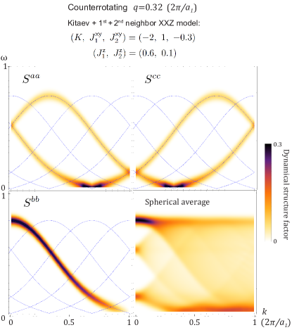
Figure 4: Dynamical structure factor signature of Kitaev exchange – plots for additional parameters. Additional structure factor plots for a model with nearest-neighbor Kitaev exchange together with smaller easy-plane $J_{1}$-$J_{2}$, with intermediate values for the easy-plane anisotropies. (Color intensity is dynamical spin structure factor, convolved with $\sigma{=}0.025$ energy Gaussian; thin blue lines are underlying spin wave dispersions.) Though the spin wave dispersions are modified, the qualitative nature of the distinctive feature remains.

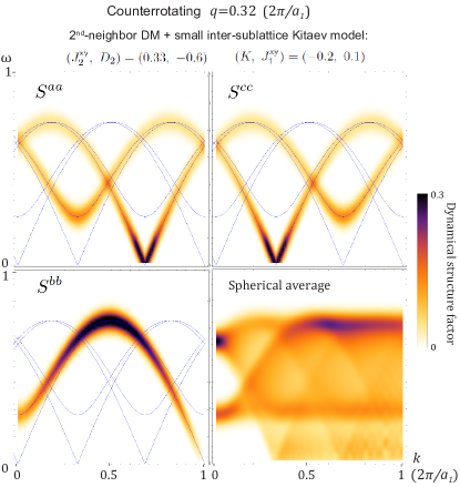
Figure 5: Dynamical structure factor for second-neighbor DM model with additional small first neighbor Kitaev-based exchange. Additional structure factor plots for a model based on the DM mechanism but with an additional perturbation. The second-neighbor DM model whose plots are shown in Fig. 3 panel (b) consists of two independent chains, the A sublattice and the B sublattice, which are fully decoupled — each sublattice has its own usual Heisenberg plus DM model, though the sublattices have opposite DM vectors. The relative phase between the two spirals is then chosen spontaneously, via spontaneous symmetry breaking of the SO(2) symmetry. Small inter-sublattice couplings will explicitly modify the ground state, but will not drastically modify the structure factor at finite energies. This can be seen explicitly by adding small coupling between the two sublattices, in the form of the Kitaev model of Fig. 3 panel (c), which fix the ground state into the Kitaev counterrotating spiral of Fig. 1 panel (a). The structure factor of the resulting model is shown here. (Color is dynamical spin structure factor, convolved with a $\sigma{=}0.025$ energy Gaussian; thin blue lines are underlying spin wave dispersions.) The $S^{aa}$ and $S^{cc}$ structure factors are no longer equal due to the presence of the Kitaev exchange. The inter-sublattice Kitaev coupling gaps out the dispersions at wavevector $q$ in $S^{aa}$ and $2\pi/a_{1}-q$ in $S^{cc}$, but as long as it is not too large, it leaves the strong intensity region of $S^{bb}$ essentially unaffected.

.3 Supplementary Material: (3) Classical solutions across the duality.

The Klein duality transforms the co-rotating spiral into the counter-rotating spiral, and vice versa, as well as exchanging wavevector $q\rightarrow 2\pi/a_{1}-q$. Here we consider these two spiral orders related by the duality in detail. In the counterrotating spiral, the spin configuration is described by the following functions, on sublattice $A$ and sublattice $B$ separately:

$$\vec{S}_{A,r} =\cos(qr)\hat{c}+\sin(qr)\hat{a}$$

$$\vec{S}_{B,r} =\cos(qr)\hat{c}-\sin(qr)\hat{a}$$ (6)

In the co-rotating spiral, the spin configuration is described by the same function on the two sublattices, i.e. the spin moment at a general site r (on either the A or B sublattice) is given by

$$\vec{S}_{r}=\cos(qr)\hat{c}-\sin(qr)\hat{a}$$ (7)

Let us consider the models with $D_{2}=0$, related by the duality. The classical energies per site of the co-rotating and counterrotating spiral models, $E_{H}$ and $E_{K}$ respectively, are given by the following (in units of $S^{2}$):

$$E_{H}=J_{1}^{\mathsf{xy}}\cos(qa_{1}/2)+J_{2}^{\mathsf{xy}}\cos(qa_{1})$$ (8)

$$E_{K}=(K/2)\sin(qa_{1}/2)+J_{2}^{\mathsf{xy}}\cos(qa_{1})$$ (9)

When parameters are taken to match under the duality relations above, the two ground state energies become identical upon the substitution $q\rightarrow\pi/a_{1}-q$.

On both sides of the duality, the incommensurate spiral with nonzero wavevector becomes the stable classical ground state for $|J_{2}^{\mathsf{xy}}|>|J_{1}^{\mathsf{xy}}|/4$. This is well known on the Heisenberg side, where this is the critical value of AF $J_{2}$ needed to frustrate the FM $J_{1}$ order. Then the spiral wavevector, determined by minimizing the energy, is as follows:

$$q_{\text{co-rot}}=\frac{2}{a_{1}}\arccos\left(\frac{|J_{1}^{\mathsf{xy}}|}{4J_{2}^{\mathsf{xy}}}\right)$$ (10)

$$q_{\text{counter-rot}}=\frac{2}{a_{1}}\arcsin\left(\frac{K}{8|J_{2}^{\mathsf{xy}}|}\right)$$ (11)

The DM-based model is straightforward; to study the effects of the duality on $D_{2}$, note that $q\rightarrow\pi/a_{1}-q$ changes the sign of the relevant quantity $\tan(qa_{1})$.

The spiral ground state of the $J_{1}$-$J_{2}$ Heisenberg model spontaneously chooses a $+q$ or $-q$ ground state, as can be seen in the $q\rightarrow-q$ symmetry of $E_{H}$ in Eq. 9. When the duality mapping is exact, this feature is preserved, though in an unusual form. The energy of the counterrotating spiral in this model, $E_{K}$ in Eq. 9, also has two solutions: wavevector $q$, as well as wavevector $2\pi/a_{1}-q$. The latter solution is the counter-rotating dual of the $-q$ co-rotating spiral. Both solutions can also be seen as allowed wavevector solutions of the right-hand-side of Eq. 11. The $q\rightarrow(2\pi/a_{1}-q)$ transformation can be enacted visually by flipping spins on one sublattice (equivalent to adding $2\pi/a_{1}$ to $q$) followed by a flip of the sense of rotation on both sublattices. In other words, the sense of the rotation in the counterrotating spiral depends on the sublattice, on the sign of the Kitaev exchange, and on whether the chosen solution involves $S^{c}$ or $S^{a}$ as the spin component which is aligned across the two sublattices. This manifestation of the $\pm q$ symmetry is a useful consistency check for the duality on these 1D models; however, it is not a robust feature on the Kitaev side of the duality, and disappears upon inclusion of inter-chain $I_{c}$ couplings which are expected to arise in certain modelsKimchi et al. (2015). These energetically favor $S^{c}$ alignment, which is equivalent to explicitly choosing one of the two solutions as the unique ground state, namely wavevector $q$ in the notation above.

.4 Supplementary Material: (4) Details of the spin wave Hamiltonian computation.

First let us recall the definition of the local coordinate system. We here write vectors in spin space using the orthorhombic axes basis $(a,b,c)$ that allows a common description of the crystal structure of all three polytypes of Li₂IrO₃. The Kitaev axes are given by $\hat{\mathsf{x}},\hat{\mathsf{y}}=(\hat{a}\pm\hat{c})/\sqrt{2}$, $\hat{\mathsf{z}}=\hat{b}$. The zigzag chains are oriented along the diagonals of the orthorhombic structural cell, with $\vec{a}_{1}=(\vec{a}\pm\vec{b})/2$, making an angle $\sim$55^∘ with the ($ac$) spin rotation plane Kimchi et al. (2015). Let site $j$ be defined by its spatial position $r$ and unit cell index $s$. The local coordinate system is written as

$$e^{3}_{r,s} =-\eta_{s}\sin(qr)\hat{a}+\cos(qr)\hat{c}$$

$$=\left\{-\eta_{s}\sin(qr),\ 0,\ \cos(qr)\right\}$$

$$e_{j}^{\pm} =\left\{\cos(qr),\ \pm i,\ \eta_{s}\sin(qr)\right\}$$ (12)

where $\eta_{s}$ is defined as follows. For the Kitaev model counterrotating spiral, $\eta_{s}=+1$ for sublattice $s=B$ and $\eta_{s}=-1$ for sublattice $s=A$. For the Heisenberg model co-rotating spiral, $\eta_{s}=+1$ independent of sublattice.

The spin wave Hamiltonian in real space is computed as follows. A useful intermediate step is the following,

$$H=\frac{1}{2}\sum_{ij}\bigg{[} \ (e^{3}_{j}{\cdot}\tilde{J}_{ij}{\cdot}e^{3}_{i})\big{(}S^{2}-S(b^{\dagger}_{j}b_{j}+b_{j}b^{\dagger}_{j}-1)\big{)}$$

$$+\frac{S}{2}\big{(}e_{j}^{-}b_{j}+e_{j}^{+}b^{\dagger}_{j}\big{)}{\cdot}\tilde{J}_{ij}{\cdot}\big{(}e_{i}^{-}b_{i}+e_{i}^{+}b^{\dagger}_{i}\big{)}\bigg{]}$$ (13)

Note that the apparent symmetry between $b$ operators left and right of $\tilde{J}$ results in the $\sigma^{1}$ term when using the $a^{\pm}$ notation. The spin wave Hamiltonian is then found within the form shown in the main text,

$$H_{\text{SW}} =\frac{1}{8}\sum_{i,j}\left[e^{\mu}_{i}{\cdot}J_{i,j}{\cdot}e^{\rho}_{j}\sigma^{1}_{\rho\nu}-4E_{\text{cl}}\delta_{\mu\nu}\delta_{ij}\right]\left(a^{\mu}_{i}\right)^{\dagger}a^{\nu}_{j}$$ (14)

where $J_{i,j}$ is the spin interaction matrix associated with Eq. 1, taken between spins $i,j$; $\sigma^{1}$ is a Pauli matrix; and summation over repeated $\mu,\nu,\rho$ indices is implied, taking values $\pm 1$. We have subtracted a total energy shift $S(S{+}1)NE_{\text{cl}}$; here $E_{\text{cl}}\equiv(1/2N_{\text{sites}})\sum_{i,j}e^{3}_{i}\cdot J_{i,j}\cdot e^{3}_{j}$ is the classical energy. Recall that in the $1/S$ spin wave expansion, $S^{3}\rightarrow 1/2-b^{\dagger}b$ and $S^{\pm}\rightarrow b,b^{\dagger}\equiv a^{\pm}$ where the $a^{\pm}$ spin wave operators are introduced for convenience.

For completeness we record the full spin interactions in the rotating frame. We write the interaction matrix in the $2\times 2$ subspace of the $\hat{a},\hat{c}$ basis, using Pauli matrices. Let us use a notation where we list the coefficients of the Identity matrix followed by the three Pauli matrices, i.e. $\sigma^{0,1,2,3}$ respectively. In this notation, the nearest neighbor lab-frame spin interactions are $(J_{1}^{\mathsf{xy}}+K/2,\eta_{s}K/2,0,0)$, while the second neighbor (intra-sublattice) lab-frame spin interactions are $(J_{2}^{\mathsf{xy}},0,i\eta_{s}D_{2},0)$. The rotating frame spin interaction matrices are then as follows. For nearest-neighbor bonds in the counterrotating spiral,

$$\tilde{J_{1}}\rightarrow\Bigg{(} \frac{K+2J_{1}^{\mathsf{xy}}}{2}\cos\left(q\frac{4r+a_{1}}{2}\right),\ \frac{1}{2}\eta_{s}K\cos\left(\frac{qa_{1}}{2}\right),$$

$$i\eta_{s}\frac{K+2J_{1}^{\mathsf{xy}}}{2}\sin\left(q\frac{4r+a_{1}}{2}\right),\ -\frac{K}{2}\sin\left(\frac{qa_{1}}{2}\right)\Bigg{)}$$ (15)

For nearest-neighbor bonds in the co-rotating spiral,

$$\tilde{J_{1}}\rightarrow\Bigg{(} \frac{K+2J_{1}^{\mathsf{xy}}}{2}\cos\left(\frac{qa_{1}}{2}\right),\ \frac{1}{2}\eta_{s}K\cos\left(q\frac{4r+a_{1}}{2}\right),$$

$$-i\eta_{s}\frac{K+2J_{1}^{\mathsf{xy}}}{2}\sin\left(\frac{qa_{1}}{2}\right),\ \frac{K}{2}\sin\left(q\frac{4r+a_{1}}{2}\right)\Bigg{)}$$ (16)

For second-neighbor bonds, which lie within a single sublattice, for either co- or counter-rotation,

$$\tilde{J_{2}}\rightarrow\bigg{(} J_{2}^{\mathsf{xy}}\cos(qa_{1})+D_{2}\sin(qa_{1}),\ 0,$$

$$i\eta_{s}(D_{2}\cos(qa_{1})-J_{2}^{\mathsf{xy}}\sin(qa_{1})),\ 0\bigg{)}$$ (17)

In each of these expressions, the diagonal matrix elements of $\tilde{J}$ with $\hat{a}$ ($\hat{c}$ ) can be read off as the sum (difference) of the identity and $\sigma^{3}$ coefficients, ie the first component plus (minus) the last component.

The momentum space spin wave Hamiltonian can be expressed as follows,

$$H_{\text{SW}}=\frac{S}{4}\sum_{k,ss^{\prime}\mu\mu^{\prime}}\ \tilde{H}^{\mu\mu^{\prime}}_{ss^{\prime}}(k)\ (a_{k,s}^{\mu})^{\dagger}\ a_{k,s^{\prime}}^{\mu^{\prime}}$$ (18)

where

$$\tilde{H}^{\mu\mu^{\prime}}_{ss^{\prime}} =-4(\hat{c}\cdot(\tilde{J_{1}}+\tilde{J_{2}})\cdot\hat{c})\nu^{0}_{\mu\mu^{\prime}}\tau^{0}_{ss^{\prime}}$$ (19)

$$+2(\hat{a}\cdot(\tilde{J_{1}}C_{1}\tau^{1}_{ss^{\prime}}+\tilde{J_{2}}C_{2}\tau^{0}_{ss^{\prime}})\cdot\hat{a})(\nu^{0}_{\mu\mu^{\prime}}+\nu^{1}_{\mu\mu^{\prime}})$$

$$+2(J_{1}^{\mathsf{z}}C_{1}\tau^{1}_{ss^{\prime}}+J_{2}^{\mathsf{z}}C_{2}\tau^{0}_{ss^{\prime}})(\nu^{0}_{\mu\mu^{\prime}}-\nu^{1}_{\mu\mu^{\prime}})$$

$$C_{\alpha} \equiv\cos\left(\frac{\alpha ka_{1}}{2}\right)$$

where $\nu$ and $\tau$ are Pauli matrices for the Bogoliubov $\mu$ and sublattice $s$ indices. The diagonal matrix elements of $\tilde{J}$ can be read off from the equations in the paragraph above, and $\tilde{J_{1}}$ and $\tilde{J_{2}}$ are the spin interactions between first and second neighbors respectively.

We may also explicitly record the matrix $\tilde{H}^{\mu\mu^{\prime}}_{ss^{\prime}}(k)$, specialized to the case of most interest, $D_{2}=0$. We define

$$L_{1}=\left(\frac{K}{2}+J_{1}^{\mathsf{xy}}\right)\cos\left(\frac{qa_{1}}{2}\right)-\frac{K}{2}\sin\left(\frac{qa_{1}}{2}\right)$$ (20)

$$L_{2}=J_{2}^{\mathsf{xy}}\cos(qa_{1})$$ (21)

With these expressions, the Hamiltonian matrix may be written as

$$\tilde{H}=A\nu^{0}\tau^{0}+B\nu^{0}\tau^{1}+C\nu^{1}\tau^{0}+D\nu^{1}\tau^{1}$$ (22)

with $A,B,C,D$ given by

$$A=-4\left(L_{2}+\zeta L_{1}\right)+2\cos(ka_{1})(L_{2}+J_{2z})$$

$$B=2\cos\left(\frac{ka_{1}}{2}\right)(L_{1}+J_{z})$$

$$C=2\cos(ka_{1})(L_{2}-J_{2z})$$

$$D=2\cos\left(\frac{ka_{1}}{2}\right)(L_{1}-J_{z})$$ (23)

The $\zeta=\pm$ sign corresponds to the Heisenberg/Kitaev cases, taking the value $\zeta=+1$ for the co-rotating spiral, and $\zeta=-1$ for the counter-rotating spiral. The sublattice indices $s,s^{\prime}$ (of the matrices $\tau$) and the Bogoliubov indices $\mu,\mu^{\prime}$ (of the matrices $\nu$) are suppressed.

.5 Supplementary Material: (5) Details of the dynamical structure factor computation.

Now we turn to computing the dynamical spin correlators. We find that the structure factor is diagonal in the $a,b,c$ basis for the spin axes, rather than the Kitaev $\mathsf{x,y,z}$ axes; only in the $a,b,c$ axes do all off-diagonal terms cancel.

The dynamical spin structure factor is expressed by the following,

$$S^{aa}(p,\omega)=\frac{S}{32}\sum_{k=\pm q}F_{(+,+)}(p+k,\omega)$$

$$S^{cc}(p,\omega)=\frac{S}{32}\sum_{k=\pm q}F_{(+,\zeta)}(p+k,\omega)$$

$$S^{bb}(p,\omega)=\frac{S}{8}F_{(-,+)}(p,\omega)$$ (24)

The differing second argument for $F$ in $S^{cc}$ for the counterrotating case arises from the product of sublattice signs $\eta_{s}\eta_{s^{\prime}}$, which arises in this case through the axis perpendicular to the local spin orientation. The function $F_{(\eta_{m},\eta_{t})}(k,\omega)$, where $\eta_{m}$ and $\eta_{t}$ are $\pm$ signs, is defined by

$$F_{(\eta_{m},\eta_{t})}(k,\omega)=\sum_{n=1,2}\delta(\omega-\omega_{n}(k))\times$$ (25)

$$\bigg{[}\sum_{ss^{\prime}\mu\mu^{\prime}}\left(T^{(-1,\mu)}_{(n,s)}(k)\right)^{\dagger}$$

$$\qquad\left(\nu^{0}{+}\eta_{m}\nu^{1}\right)_{\mu\mu^{\prime}}\left(\tau^{0}{+}\eta_{t}\tau^{1}\right)_{ss^{\prime}}\left(T^{(\mu^{\prime},-1)}_{(s^{\prime},n)}(k)\right)\bigg{]}$$

here $n$ labels the two bands of the spin wave dispersion at positive energies, and $T$ is the diagonalizing transformation matrix, defined by $a=T\cdot\alpha$, such that

$$a^{\mu}_{s,k}=\sum_{s^{\prime},\mu^{\prime}}\left(T^{(\mu,\mu^{\prime})}_{(s,s^{\prime})}(k)\right)\alpha^{\mu^{\prime}}_{s^{\prime},k}$$

where $\alpha$ are the Bogoliubov-diagonalized excitations, and $\mu^{\prime}=-1$ refers to the second component of the vector $\alpha$. The Bogoliubov transformation $T$ was computed numericallyMaestro and Gingras (2004). To compute the eigenvalues, it is sufficient to simply diagonalize $H(k)\nu^{3}$.

References

- Wen (2004) X.-G. Wen, Quantum Field Theory of Many-Body Systems (Oxford University Press, 2004).
- Note (1) For a few recent reviews see Refs. \rev@citealpBalents2014, Kee2016, LucilleReview2016, Ng2016.
- Singh and Gegenwart (2010) Y. Singh and P. Gegenwart, Phys. Rev. B 82, 064412 (2010).
- Liu et al. (2011) X. Liu, T. Berlijn, W.-G. Yin, W. Ku, A. Tsvelik, Y.-J. Kim, H. Gretarsson, Y. Singh, P. Gegenwart, and J. P. Hill, Phys. Rev. B 83, 220403 (2011).
- Ye et al. (2012) F. Ye, S. Chi, H. Cao, B. C. Chakoumakos, J. A. Fernandez-Baca, R. Custelcean, T. F. Qi, O. B. Korneta, and G. Cao, Phys. Rev. B 85, 180403 (2012).
- Choi et al. (2012) S. K. Choi, R. Coldea, A. N. Kolmogorov, T. Lancaster, I. I. Mazin, S. J. Blundell, P. G. Radaelli, Y. Singh, P. Gegenwart, K. R. Choi, S.-W. Cheong, P. J. Baker, C. Stock, and J. Taylor, Phys. Rev. Lett. 108, 127204 (2012).
- Singh et al. (2012) Y. Singh, S. Manni, J. Reuther, T. Berlijn, R. Thomale, W. Ku, S. Trebst, and P. Gegenwart, Phys. Rev. Lett. 108, 127203 (2012).
- Plumb et al. (2014) K. W. Plumb, J. P. Clancy, L. J. Sandilands, V. V. Shankar, Y. F. Hu, K. S. Burch, H.-Y. Kee, and Y.-J. Kim, Phys. Rev. B 90, 041112 (2014).
- Sears et al. (2015) J. A. Sears, M. Songvilay, K. W. Plumb, J. P. Clancy, Y. Qiu, Y. Zhao, D. Parshall, and Y.-J. Kim, Phys. Rev. B 91, 144420 (2015).
- Majumder et al. (2015) M. Majumder, M. Schmidt, H. Rosner, A. A. Tsirlin, H. Yasuoka, and M. Baenitz, Phys. Rev. B 91, 180401 (2015).
- Johnson et al. (2015) R. D. Johnson, S. C. Williams, A. A. Haghighirad, J. Singleton, V. Zapf, P. Manuel, I. I. Mazin, Y. Li, H. O. Jeschke, R. Valentí, and R. Coldea, Phys. Rev. B 92, 235119 (2015).
- Sandilands et al. (2015) L. J. Sandilands, Y. Tian, K. W. Plumb, Y.-J. Kim, and K. S. Burch, Phys. Rev. Lett. 114, 147201 (2015).
- Sandilands et al. (2016) L. J. Sandilands, Y. Tian, A. A. Reijnders, H.-S. Kim, K. W. Plumb, Y.-J. Kim, H.-Y. Kee, and K. S. Burch, Phys. Rev. B 93, 075144 (2016).
- Banerjee et al. (2016) A. Banerjee, C. A. Bridges, J.-Q. Yan, A. A. Aczel, L. Li, M. B. Stone, G. E. Granroth, M. D. Lumsden, Y. Yiu, J. Knolle, S. Bhattacharjee, D. L. Kovrizhin, R. Moessner, D. A. Tennant, D. G. Mandrus, and S. E. Nagler, Nature Materials 15, 733 (2016).
- Modic et al. (2014) K. A. Modic, T. E. Smidt, I. Kimchi, N. P. Breznay, A. Biffin, S. Choi, R. D. Johnson, R. Coldea, P. Watkins-Curry, G. T. McCandless, J. Y. Chan, F. Gandara, Z. Islam, A. Vishwanath, A. Shekhter, R. D. McDonald, and J. G. Analytis, Nat Commun 5, 4203 (2014).
- Takayama et al. (2015) T. Takayama, A. Kato, R. Dinnebier, J. Nuss, H. Kono, L. S. I. Veiga, G. Fabbris, D. Haskel, and H. Takagi, Phys. Rev. Lett. 114, 077202 (2015).
- Biffin et al. (2014a) A. Biffin, R. D. Johnson, I. Kimchi, R. Morris, A. Bombardi, J. G. Analytis, A. Vishwanath, and R. Coldea, Phys. Rev. Lett. 113, 197201 (2014a).
- Biffin et al. (2014b) A. Biffin, R. D. Johnson, S. Choi, F. Freund, S. Manni, A. Bombardi, P. Manuel, P. Gegenwart, and R. Coldea, Phys. Rev. B 90, 205116 (2014b).
- Williams et al. (2016) S. C. Williams, R. D. Johnson, F. Freund, S. Choi, A. Jesche, I. Kimchi, S. Manni, A. Bombardi, P. Manuel, P. Gegenwart, and R. Coldea, Phys. Rev. B 93, 195158 (2016).
- Takayama (2016) T. Takayama, Invited Talk, American Physical Society March Meeting (2016).
- Knolle et al. (2014) J. Knolle, D. L. Kovrizhin, J. T. Chalker, and R. Moessner, Phys. Rev. Lett. 112, 207203 (2014).
- Knolle et al. (2015) J. Knolle, D. L. Kovrizhin, J. T. Chalker, and R. Moessner, Phys. Rev. B 92, 115127 (2015).
- Smith et al. (2016) A. Smith, J. Knolle, D. L. Kovrizhin, J. T. Chalker, and R. Moessner, Phys. Rev. B 93, 235146 (2016).
- Nasu et al. (2016) J. Nasu, J. Knolle, D. L. Kovrizhin, Y. Motome, and R. Moessner, Nature Physics 12, 912 (2016), arXiv:1602.05277 [cond-mat.str-el] .
- Song et al. (2016) X.-Y. Song, Y.-Z. You, and L. Balents, Phys. Rev. Lett. 117, 037209 (2016).
- Kimchi et al. (2014) I. Kimchi, J. G. Analytis, and A. Vishwanath, Phys. Rev. B 90, 205126 (2014).
- Toth and Lake (2015) S. Toth and B. Lake, Journal of Physics Condensed Matter 27, 166002 (2015), arXiv:1402.6069 [cond-mat.str-el] .
- Damay et al. (2010) F. m. c. Damay, C. Martin, V. Hardy, A. Maignan, G. André, K. Knight, S. R. Giblin, and L. C. Chapon, Phys. Rev. B 81, 214405 (2010).
- Kitaev (2006) A. Kitaev, Annals of Physics 321, 2 (2006).
- Jackeli and Khaliullin (2009) G. Jackeli and G. Khaliullin, Phys. Rev. Lett. 102, 017205 (2009).
- Chaloupka et al. (2010) J. Chaloupka, G. Jackeli, and G. Khaliullin, Phys. Rev. Lett. 105, 027204 (2010).
- Hwan Chun et al. (2015) S. Hwan Chun, J.-W. Kim, J. Kim, H. Zheng, C. C. Stoumpos, C. D. Malliakas, J. F. Mitchell, K. Mehlawat, Y. Singh, Y. Choi, T. Gog, A. Al-Zein, M. M. Sala, M. Krisch, J. Chaloupka, G. Jackeli, G. Khaliullin, and B. J. Kim, Nat Phys 11, 462 (2015).
- Rau et al. (2014) J. G. Rau, E. K.-H. Lee, and H.-Y. Kee, Phys. Rev. Lett. 112, 077204 (2014).
- Lee and Kim (2015) E. K.-H. Lee and Y. B. Kim, Phys. Rev. B 91, 064407 (2015).
- Kimchi and Vishwanath (2014) I. Kimchi and A. Vishwanath, Phys. Rev. B 89, 014414 (2014).
- Sup (rial) See the Supplemental Material of this manuscript for details (Supplemental Material).
- Lee et al. (2016) E. K.-H. Lee, J. G. Rau, and Y. B. Kim, Phys. Rev. B 93, 184420 (2016).
- Khaliullin and Okamoto (2002) G. Khaliullin and S. Okamoto, Phys. Rev. Lett. 89, 167201 (2002).
- Khaliullin and Okamoto (2003) G. Khaliullin and S. Okamoto, Phys. Rev. B 68, 205109 (2003).
- Khaliullin (2005) G. Khaliullin, Progress of Theoretical Physics Supplement 160, 155 (2005).
- Chaloupka et al. (2013) J. Chaloupka, G. Jackeli, and G. Khaliullin, Phys. Rev. Lett. 110, 097204 (2013).
- Reuther et al. (2012) J. Reuther, R. Thomale, and S. Rachel, Phys. Rev. B 86, 155127 (2012).
- Li et al. (2015) K. Li, S.-L. Yu, and J.-X. Li, New Journal of Physics 17, 043032 (2015).
- Winter et al. (2016) S. M. Winter, Y. Li, H. O. Jeschke, and R. Valentí, Phys. Rev. B 93, 214431 (2016).
- Kimchi et al. (2015) I. Kimchi, R. Coldea, and A. Vishwanath, Phys. Rev. B 91, 245134 (2015).
- Maestro and Gingras (2004) A. G. D. Maestro and M. J. P. Gingras, Journal of Physics: Condensed Matter 16, 3339 (2004).
- Witczak-Krempa et al. (2014) W. Witczak-Krempa, G. Chen, Y. B. Kim, and L. Balents, Annual Review of Condensed Matter Physics 5, 57 (2014), http://dx.doi.org/10.1146/annurev-conmatphys-020911-125138 .
- Rau et al. (2016) J. G. Rau, E. K.-H. Lee, and H.-Y. Kee, Annual Review of Condensed Matter Physics 7, 195 (2016), arXiv:1507.06323 [cond-mat.str-el] .
- Savary and Balents (2016) L. Savary and L. Balents, ArXiv e-prints (2016), arXiv:1601.03742 [cond-mat.str-el] .
- Zhou et al. (2016) Y. Zhou, K. Kanoda, and T.-K. Ng, ArXiv e-prints (2016), arXiv:1607.03228 [cond-mat.str-el] .