Magnetic Suppression of Turbulence and the Star Formation Activity of Molecular Clouds

Abstract

We present magnetohydrodynamic simulations aimed at studying the effect of the magnetic suppression of turbulence (generated through various instabilities during the formation of molecular clouds by converging) on the subsequent star formation (SF) activity. We study four magnetically supercritical models with magnetic field strengths $B=0$, 1, 2, and 3 $\mu$G (corresponding to mass–to–flux ratios of $\infty$, 4.76, 2.38, and 1.59 times the critical value), with the magnetic field, initially being aligned with the flows. We find that, for increasing magnetic field strength, the clouds formed tend to be more massive, denser, less turbulent, and with higher SF activity. This causes the onset of star formation activity in the non–magnetic or more weakly magnetized cases to be delayed by a few Myr in comparison to the more strongly magnetized cases. We attribute this behavior to the suppression of the nonlinear thin shell instability (NTSI) by the magnetic field, previously found by Heitsch and coworkers. This result is contrary to the standard notion that the magnetic field provides support to the clouds, thus reducing their star formation rate (SFR). However, our result is a completely nonlinear one, and could not be foreseen from simple linear considerations.

1 Introduction

The effect of magnetic fields on the evolution of molecular clouds (MCs) is not yet fully understood, in particular concerning its effect on the formation of the clouds and their subsequent star formation (SF) processes (see e.g., Passot et al., 1995; Hennebelle & Pérault, 2000; Hartmann et al., 2001; Ostriker et al., 2001; Kim et al., 2003; Inoue & Inutsuka, 2008, 2009, 2012; Heitsch et al., 2009; Banerjee et al., 2009; Vázquez-Semadeni et al., 2011; Inutsuka et al., 2015; Körtgen & Banerjee, 2015).

One scenario that has been recently proposed for the formation of MCs (in solar neighborhood–like conditions) is that of colliding flows, in which moderately supersonic streams of warm neutral medium (WNM) collide to produce a cold neutral cloud through nonlinear triggering of the thermal instability (TI; Ballesteros-Paredes et al., 1999; Hennebelle & Pérault, 1999). The cloud becomes turbulent through the combined action of TI and various other dynamical instabilities, such as the nonlinear thin shell (NTSI), Kelvin-Helmholtz, and Rayleigh-Taylor instabilities (see e.g., Vishniac, 1994; Koyama & Inutsuka, 2002; Heitsch et al., 2006; Vázquez-Semadeni et al., 2006). Moreover, as a cloud forms and grows out of compression in the WNM, it should become molecular, supercritical, and gravitationally unstable at roughly the same time (see e.g., Hartmann et al., 2001), transiting to a regime of gravitational collapse. Because this mechanism can coherently produce large amounts of cold, dense gas, the newly formed clouds may contain numerous Jeans masses, and thus the collapse can proceed in a hierarchical fashion, roughly as predicted by Hoyle (1953), but aided by the fact that the cloud’s internal turbulence produces nonlinear density fluctuations that have shorter free-fall times than the cloud at large (Heitsch & Hartmann, 2008; Vázquez-Semadeni et al., 2009; Gómez & Vázquez-Semadeni, 2014; Vázquez-Semadeni, 2015). This mechanism provides a self-consistent way to generate the observed structure and dynamics of MCs and to regulate the evolution of the star formation rate (SFR) (e.g., Zamora-Avilés et al., 2012; Zamora-Avilés & Vázquez-Semadeni, 2014).

However, as the magnetic field is ubiquitous in the Galaxy, it is expected to play a central role in the formation of clouds. Hennebelle (2013) showed that regardless of the initial conditions (decaying turbulence or converging flows), the magnetic field increases the number of and builds more defined filamentary structures due to the magnetic tension. These filaments also live longer.

The “magnetic criticality” is an important concept we will refer throughout the paper. To define it, we first define the mass–to–flux ratio (M2FR) as $\mu=\Sigma/\langle B_{x}\rangle$, where $\langle B_{x}\rangle$ is the mean magnetic field along the $x$–direction and $\Sigma$ is the surface density measured along the same direction and covering the entire length and cross section of the inflows (see Sec. 3.4; see also Banerjee et al., 2009; Vázquez-Semadeni et al., 2011). We then refer to magnetically supercritical/subcritical clouds if the M2FR is greater/lower than the critical value, $\mu_{\rm crit}=0.16/\sqrt{G}$, which is an appropriate estimate for sheet-like clouds (Nakano & Nakamura, 1978) as those studied here.

In the case of converging flows, the strength and orientation of the mean magnetic field with respect to the flows play a crucial role for the flow-driven formation of MCs, in particular for whether the clouds can become dense, massive and supercritical (e.g., Elmegreen, 1994; Passot et al., 1995; Hennebelle & Pérault, 2000; Hartmann et al., 2001; Inoue & Inutsuka, 2008, 2009, 2012; Heitsch et al., 2009; Banerjee et al., 2009; Vázquez-Semadeni et al., 2011; Heitsch & Hartmann, 2014; Lazarian, 2014; Körtgen & Banerjee, 2015). This is simply because the gas can flow freely along field lines, but in the perpendicular direction it is opposed by the magnetic pressure, and because coherent compressions are sometimes deemed difficult to maintain over the required scales of hundreds of parsecs. Moreover, the magnetic tension tends to weaken or even suppress the dynamical instabilities (and thus the generation of turbulence) in the clouds assembled by colliding flows, particularly the NTSI (Heitsch et al., 2007; Heitsch et al., 2009) by preventing the transport of transverse momentum.

When the magnetic field is aligned with the WNM inflows, Heitsch et al. (2007) using pressure considerations and 2D simulations, found that the NTSI is suppressed if the Alfvén speed ($v_{\rm A}$) becomes comparable to the inflow velocity. Moreover, Heitsch et al. (2009), using numerical simulations of colliding flows, found that both the strength and orientation of the magnetic field with respect to the inflows determine the morphology, thermal state, and the dynamics of MC precursors. Note that those authors did not include self-gravity in their analysis, and thus they did not study the resulting SF activity.

Banerjee et al. (2009) simulated the assembly of MCs by converging flows in a weakly magnetized medium including self–gravity. They studied the thermal and dynamical properties of clumps, finding that once the clumps are formed by the TI, they grow in mass and size by accretion from the WNM and eventually become Jeans unstable. They found that the star formation efficiency (SFE) reaches $\sim 50$% at the end of the simulation. Vázquez-Semadeni et al. (2011) extended the latter work to explore higher magnetic field strengths (studying three models: one supercritical and two subcritical) and by taking into account diffusive processes, concluding that the SF activity is strongly attenuated in the subcritical cases by preventing the global collapse of the cloud. On the other hand, these authors reported an SFE of $\sim 40$% in the supercritical case. Finally, Körtgen & Banerjee (2015) presented a parameter study aimed at studying the transition from magnetically sub– to super–critical states of cores immersed in subcritical clouds, finding that this is difficult to achieve even taking into account non–ideal MHD effects. Thus, the preferred mechanism for producing super-critical objects is by accretion from long distances, as described in Hartmann et al. (2001) and Vázquez-Semadeni et al. (2011). However, note that, although the clouds studied by Körtgen & Banerjee (2015) are globally supported by magnetic fields, they exhibit a strong turbulence suppression, particularly in models in which the inflows are aligned with the magnetic field lines (see their Fig. 12 and Table 1 below). This can be interpreted at the same time as an annihilation of the NTSI since the magnetic pressure overwhelmingly dominates the turbulent ram pressure (as pointed out by Heitsch et al., 2007).

In this contribution, we extend the previous works of Heitsch et al. (2007); Heitsch et al. (2009) by including self-gravity and modeling the SF process. We also extend the models by Banerjee et al. (2009); Vázquez-Semadeni et al. (2011); Körtgen & Banerjee (2015) by studying four magnetically supercritical clouds, focusing in the effect of magnetic suppression of turbulence on the SF activity (see Table 1 for a comparison of the initial conditions used in each work).

Finally, the plan of the paper is as follows: In Section 2 we briefly describe the main instabilities occurring during the formation of MCs by converging flows. In Section 3 we describe the numerical model. The results are presented in Sec. 4 and discussed in Sec. 5. Finally, a summary and some conclusions are presented in Section 6.

Table 1: Overview of the initial conditions used in works with similar setup, i.e., two WNM colliding flows aligned with the magnetic field (see Sec. 3.4 for a detailed description). Here, $n_{0}$ is the initial number density, $c_{\rm s}$ the isothermal sound speed of the WNM, $v_{\rm inf}$ the inflow velocity, $R_{\rm inf}$ is half of the inflow diameter (the inflow length, $L_{\rm inf}$, is 112 pc in all works, except in Heitsch et al. (2009) since they consider inflow boundary conditions), $\mathcal{M}_{\rm rms}$ is the background turbulence, $|B_{0}|$ is the initial magnetic field strength, $\mu$ the mass–to–flux ratio (M2FR), and $v_{\rm A}$ the alfvén speed ($=B_{0}/\sqrt{4\pi\rho}$).

	$n_{0}$	$c_{\rm s}$	$v_{\rm inf}$	$R_{\rm inf}$		$|B_{0}|$
	(${\rm cm}^{-3}$)	(${\rm km\leavevmode\nobreak\ s}^{-1}$)	(${\rm km\leavevmode\nobreak\ s}^{-1}$)	(pc)	$\mathcal{M}_{\rm rms}$	($\mu{\rm G}$)	$\mu/\mu_{\rm crit}$a	$v_{\rm A}/v_{\rm inf}$b
Heitsch et al. (2009)	1	7.2	16.0	22	-	0,2.5,5.0	-	0,0.3,0.6
Banerjee et al. (2009)	1	5.7	7.1	32	0.12	1	$2.37$	0.27
Vázquez-Semadeni et al. (2011)	1	5.7	13.9	32	0.12	2,3,4	$1.36$,0.91,0.68	0.27,0.42,0.56
Körtgen & Banerjee (2015)	1	5.7	11.4	64	0.4,0.4,0.5c	3,4,5c	0.79,0.59,0.47c	0.5,0.67,0.84c
This work	2	3.1	7.5	32	0.7	0,1,2,3	$\infty,4.76,2.38,1.59$d	0,0.18,0.36,0.54b

• The bold numbers correspond to magnetically supercritical models.

• Heitsch et al. (2007) found that the NTSI is supressed when $v_{\rm A}/v_{\rm inf}\gtrsim 1$ (i.e., when the magnetic pressure overcomes the tangential component of the ram pressure). According to this criterion we expect the development of the NTSI in all the models considered here (see Table 2).

• These models are labeled as B3M0.4I0, B4M0.4I0, and B5M0.5I0, respectively, in Körtgen & Banerjee (2015).

• Note that in this work, the initial density is $n_{0}=2$ cm^-3, which increases the magnetic criticality ($\mu/\mu_{\rm crit}$) by a factor of 2 with respect to previous works using instead $n_{0}=1$ cm^-3 (but the same magnetic field strength and inflow dimensions).

2 Overview of instabilities

Several instabilities enable the condensation and fragmentation of clouds formed by colliding flows, driving turbulent motions in the compressed, cooled layer. Here we briefly review the basics of the thermal, nonlinear thin-shell, Kelvin-Helmholtz and Jeans instabilities. For a more detailed discussion see e.g., Heitsch et al. (2006); Heitsch et al. (2008); Vázquez-Semadeni (2015) and references therein.

2.1 Nonlinear Thin-Shell Instability (NTSI)

In the hydrodynamic (HD) limit, the NTSI (Vishniac, 1994) is triggered in a bent cold slab formed by two accretion shocks when the slab displacement, $\eta$, is comparable to its thickness. The growth rate is $c_{\rm s}k(k\eta)^{1/2}$, where $k$ is the wave number of the slab perturbation and $c_{\rm s}$ the sound speed.

The NTSI acts by increasing the curvature of bending perturbations on the boundary of the dense compressed layer and pushing the gas towards the nodes of these perturbations. The gas therefore moves in a direction oblique to the inflows, effectively transferring part of the momentum from the inflows to the direction perpendicular to them (Vishniac, 1994). The oblique convergence of gas at opposite sides of the nodes finally results in a compression and acceleration of the gas in the nodes parallel to the inflows, but moving in the opposite direction, which ultimately produces an expansion of the layer (e.g., Folini & Walder, 2006).

On the other hand, in the MHD regime it is expected that magnetic fields soften the NTSI via the magnetic pressure term of the Lorentz force. Thus, in the configuration studied here, when the magnetic field is aligned with the inflows, the magnetic tension force prevents motions perpendicular to the magnetic field and it can even suppress the NTSI when the Alfvén speed becomes comparable to the inflow velocity (Heitsch et al., 2008).

2.2 Kelvin-Helmholtz Instability (KHI)

The KHI (see e.g., Chandrasekhar, 1961) is a velocity-shear instability, which is also expected to appear in WNM converging flows as an important turbulence driver in the MC precursors.

In the compressible HD regime, when the velocity shear is in a single continuous fluid, the instability growth rate is given by $k\Delta U$, where $k$ is the wave number of the perturbation and $\Delta U$ is the velocity jump across the shear layer. In the MHD limit, when the magnetic field is uniform and parallel to the shear flow, the magnetic tension force can reduce or even stabilize the growth rate when the velocity jump is less than the Alfvén speed (Heitsch et al., 2006, and references therein).

2.3 Thermal Instability (TI)

This instability is closely related to the cooling and heating processes. The functional form of the cooling function (which we discuss in Sec. 3.2) causes an atypical thermodinamical behavior in the ISM known as TI (Field, 1965). This instability can be understood as the tendency of the ISM to depart from the thermal equilibrium condition upon a perturbation, thus producing condensations of cold and dense regions immersed in a WNM. In the linear regime, the condensations can survive at scales ($\lambda$) smaller than the sound crossing length $\lambda_{\rm s}=\tau_{\rm c}c_{\rm s}$, $\tau_{c}$ being the cooling timescale and $c_{\rm s}$ the adiabatic sound speed. The cooling timescale is:

$$\tau_{c}=\frac{3}{2}\frac{k_{\rm B}T}{|\Gamma-n\Lambda|},$$ (1)

where $k_{\rm B}$ is the Boltzmann constant, $T$ the temperature, and $\Gamma$ and $\Lambda$ the heating and cooling functions, respectively. This instability is important in early stages of cloud formation since it is an efficient mechanism to generate non linear density perturbations and turbulence on small scales. Note, however, that turbulence can affect the behavior of the TI at pc-scales. In this regard, Sánchez-Salcedo et al. (2002) have shown that if the velocity fluctuations are dominated by the turbulence rather than by the adiabatic sound speed the growth of the perturbations can be suppressed even though $\lambda<\lambda_{\rm s}$.

2.4 Jeans instability

This well known instability occurs in a self-gravitating uniform medium (with density $\rho_{0}$), in the presence of thermal pressure, to which linear sinusoidal perturbations are added. In this case, pertubations of wavelength larger than the so-called Jeans length (Jeans, 1902)

$$\lambda_{\rm J}=\Big{(}\frac{\pi c^{2}_{\rm s}}{G\rho_{0}}\Big{)},$$ (2)

cannot be supported by the pressure gradient and proceed to collapse.

3 Numerical model

3.1 Numerical scheme

We use the Eulerian adaptive mesh refinement FLASH2.5 code (Fryxell et al., 2000) to perform three-dimensional, self gravitating, idela MHD simulations, including heating and cooling processes. The ideal MHD equations are solved using the MHD HLL3R solver, which preserves positive states for density and internal energy (Bouchut et al., 2007, 2010; Waagan, 2009; Waagan et al., 2011). This solver is suitable for highly supersonic astrophysical problems, such as those studied here.

3.2 Heating and Cooling

We calculate the heating and cooling rates using the analytic fits by Koyama & Inutsuka (2002) for the heating ($\Gamma_{\rm KI}$) and cooling ($\Lambda_{\rm KI}$) functions (see also Vázquez-Semadeni et al., 2007, for corrections to typographical errors),

$$\Gamma_{\rm KI}=2.0\times 10^{-26}\,{\rm erg}\,{\rm s}^{-1},$$ (3)

$$\frac{\Lambda_{\rm KI}(T)}{\Gamma_{\rm KI}}=10^{7}\exp\Big{(}{\frac{-1.184\times 10^{5}}{T+1000}}\Big{)}+\\ +1.4\times 10^{-2}\sqrt{T}\exp\Big{(}{\frac{-92}{T}}\Big{)}{\rm\leavevmode\nobreak\ cm}^{3},$$ (4)

which are based on the thermal and chemical calculations considered by Wolfire et al. (1995) and Koyama & Inutsuka (2000).

In the present study, we have chosen not to include any form of stellar feedback, in order to isolate the effects of varying the magnetic field. A study including stellar feedback will be presented elsewhere.

3.3 Refinement criterion and sink particles

In order to follow the development of high density regions, we employ a refinement criterion which, however, is not standard. The most frequently used criterion for refinement is the so-called Jeans criterion (Truelove et al., 1997), which aims to prevent artificial fragmentation, requiring that the local Jeans length be resolved by at least a certain minimum of grid cells. Because, at constant temperature, the Jeans length scales as $\rho^{-1/2}$, the condition of a fixed number of cells per Jeans length implies that the grid size also scales with density as $\Delta x\propto\rho^{-1/2}$. Instead, we have used a constant mass criterion, in which the grid size scales with density as $\Delta x\propto\rho^{-1/3}$, and so the mass of the new level of refined cells is the same as that of the previous level when it was created. In section 5.2 we show that the effect in using the constant mass (in run B3) instead of the Jeans criterion (run B3J) is just a delay in the onset of star formation by $\sim 10$%. Therefore, we do not consider that the usage of this criterion has any important consequences, since we are not concerned with the mass distribution of the sinks (related to the fragmentation), but only with the net SFR.

Once the maximum refinement level is reached in a given cell, a sink particle can be formed when the density in this cell exceeds a threshold number density, $\rho_{\rm thr}=8.9\times 10^{-18}\,{\rm g\leavevmode\nobreak\ cm}^{-3}$ ($=4.2\times 10^{6}\,{\rm cm}^{-3}$), among other sink-formation tests (for a detailed description and the implementation in the FLASH code, see Federrath et al., 2010). The sink is formed with the excess mass within the cell, that is, $M_{\rm Sink}=(\rho-\rho_{\rm thr})\Delta x^{3}$. The sink particles can then accrete mass (with $\rho>\rho_{\rm thr}$) from their surroundings (within an accretion radius of $\sim 2.5\Delta x$; Federrath et al., 2010).

3.4 Initial conditions

We use a setup similar to that of Vázquez-Semadeni et al. (2007). The numerical periodic box, of dimensions $L_{x}=256\,{\rm pc}$ and $L_{y}=L_{z}=128\,{\rm pc}$, is initially filled with warm neutral gas at a uniform density $n=2\,{\rm cm}^{-3}$ and constant temperature of $1450\,{\rm K}$, which corresponds to thermal equilibrium and implies an isothermal sound speed of 3.1 ${\rm km\leavevmode\nobreak\ s}^{-1}$. Assuming a composition of atomic hydrogen only (with a mean molecular weight $\mu=1.27$), the gas mass in the whole box is $\sim 2.6\times 10^{5}\,M_{\odot}$, whereas the mass contained in the cylinders is $\sim 4.5\times 10^{4}\,M_{\odot}$.

In order to trigger the NTSI, we impose an initial turbulent velocity field, which corresponds to a Burgers turbulence, with a power spectrum of $k^{-2}$ and Mach number of $\mathcal{M}_{\rm rms}\simeq$0.7. No forcing is applied at later times and therefore the turbulence decays. On top of this weak background turbulent field, we add two cylindrical streams, each of radius $R_{\rm inf}=32\,{\rm pc}$ and length $L_{\rm inf}=112\,{\rm pc}$, moving in opposite directions at a moderately supersonic velocity of $7.5\,{\rm km\leavevmode\nobreak\ s}^{-1}$ in the $x$-direction (implying a Mach number $\mathcal{M}_{\rm inf}\simeq$ 2.4 with respect to the isothermal sound speed in the WNM).

The numerical box is permeated with a uniform magnetic field along the $x$-direction, for which we consider three different strengths ($1$, $2$, and $3\,\mu{\rm G}$), along with a nonmagnetic case. Note that the corresponding mass-to-flux ratios are greater than the critical value, so that our clouds are magnetically supercritical in all cases, in agreement with observations that suggest that MCs are in general magnetically supercritical (Crutcher et al., 2010). Table 2 gives a summary of the magnetic parameters of the simulations. Finally, the maximum resolution reached is $\Delta x=0.03\,{\rm pc}$.

With this setup and initial conditions we perform four (otherwise identical) simulations, varying only the magnetic field strength. We only consider the case where the magnetic field is initially aligned with the inflows (along the $x$ direction), but note that non-aligned cases can lead to motions along the magnetic field for sufficiently high inflow speeds at a given field strength (see e.g., Hennebelle & Pérault, 2000; Körtgen & Banerjee, 2015).

Table 2: List of simulations

Run name	$|{\rm B}_{x,0}|\,(\mu{\rm G})$	$\mu/\mu_{\rm crit}$a	Refinement criterionb
B0	$0$	$\infty$	constant mass
B1	$1$	$4.76$	constant mass
B2	$2$	$2.38$	constant mass
B3	$3$	$1.59$	constant mass
B3J	$3$	$1.59$	Jeans

• Note that all the models are magnetically supercritical.

• See Section 5.2 for a discussion about the refinement criteria.

4 Results

Henceforth, the analysis focuses on the “central box” of the simulation, a cylindrical region of radius 40 pc and length of $80\,{\rm pc}$, centered at the plane where the flows collide. We will refer to the cold cloud formed in this box as the “central cloud”, or simply, “the cloud”, and here we will consider its global physical properties.

Face-on and edge-on column density views of the “central clouds” at $t=5$, $10$, $15$, and $19\,{\rm Myr}$. The different columns represent the models B0 ($B_{x,0}=0\,\mu{\rm G}$), B1 ($1\,\mu{\rm G}$), B2 ($2\,\mu{\rm G}$), and B3 ($3\,\mu{\rm G}$). The dots (in panels at $t=15$ and $19\,{\rm Myr}$) represent the projected position of the sink particles, i.e., collapsed objects. The box is $80\,{\rm pc}$ per side. Note that in the simulations with larger magnetic field strengths, the clouds are more coherent and compact.

4.1 Global evolution

The collision of WNM streams (or inflows) in the center of the numerical box nonlinearly triggers thermal instability (TI), forming a thin cloud of cold atomic gas (see e.g., Hennebelle & Pérault, 1999; Koyama & Inutsuka, 2000, 2002; Walder & Folini, 2000), which at the same time becomes turbulent by the combined action of TI with various other dynamical instabilities (see e.g., Hunter et al., 1986; Vishniac, 1994; Koyama & Inutsuka, 2002; Heitsch et al., 2005; Vázquez-Semadeni et al., 2006). Also, the total (thermal plus ram) pressure in the dense gas is in balance with the total pressure of the surrounding WNM, while the thermal pressures are also equal because of the rapid condensation caused by TI. It was shown by Banerjee et al. (2009) that the two conditions combined imply similar turbulent Mach numbers in both the diffuse and the dense gas, and so the cold, dense gas exhibits a moderately supersonic velocity dispersion. Since we do not follow the chemistry we indistinctly will refer to the dense gas ($n>100\,{\rm cm}^{-3}$) as “molecular”.

Figure 1: Same as Fig. 4, but at $t=25\,{\rm Myr}$. By this time, runs B2 and B3 have already been terminated.

Since our numerical boxes are magnetically supercritical (see Table 2), the clouds soon become dominated by self-gravity and begin to contract gravitationally as a whole. During the large-scale contraction, the local, nonlinear (i.e., large-amplitude) density enhancements produced by the initial turbulence manage to complete a collapse of their own, since their local free-fall time is shorter than the average one for the entire cloud (Vázquez-Semadeni et al., 2007; Vázquez-Semadeni et al., 2009; Heitsch & Hartmann, 2008; Pon et al., 2011). These local collapses involve only a small fraction of the cloud’s total mass (see Sec. 4.5).

4.2 Cloud structure

Figures 4 and 1 illustrate the morphological effects of magnetic fields at $t=5$, 10, 15, 19, and 25 Myr. In Fig. 4 we show $t=19$ Myr rather than 20 Myr in order to show all four simulations, since run B2 terminates before this time.

In these figures, the various columns from left to right represent column density maps of the “central clouds” for models B0, B1, B2, and B3 ($B_{x,0}=0$, $1$, $2$, and $3\,\mu{\rm G}$, respectively) in face-on and edge-on views. The morphologies (in column density maps) are consistent with those reported by Heitsch et al. (2009, see their models H, X25, and X50 in their Figure 1).

From these figures, it is seen that increasing the magnetic field strength prevents the cloud from reexpanding in the direction of the inflows, as well as from growing in the direction perpendicular to them after they collide. This can be interpreted as an inhibition of the NTSI by the magnetic field (see also, Heitsch et al., 2007; Heitsch et al., 2009). We speculate that this occurs because the magnetic field, which is parallel to the inflows, inhibits the transverse motions that would develop as a consequence of the NTSI,and therefore allows for more efficient dissipation of the inflow kinetic energy by forcing a more focused collision of the two streams.

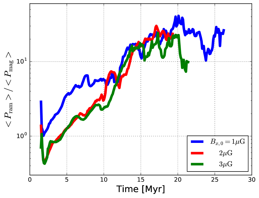
Figure 2: Time evolution of the ratio of ram to magnetic pressure (arithmetically averaged).

To test for this speculation, in Fig. 2 we plot the aritmetic average of the ram to magnetic pressure ratio ($\beta_{\rm ram}\equiv P_{\rm ram}/P_{\rm mag}$) in the dense slab ($n\gtrsim 100\,{\rm cm}^{-3}$) for models B1, B2, and B3. Based on simple pressure arguments, we expect the development of the NTSI roughly when $\beta_{\rm ram}>1$ (Heitsch et al., 2007). Thus, for model B1 the NTSI operates readily once the slab forms, whereas for models B2 and B3 the instability starts to act after $t\sim 5\,{\rm Myr}$. Interestingly, and regardless of the model, the ram pressure increases by roughly three orders of magnitude throughout the cloud evolution, whereas the magnetic pressure increases smoothly by only one order of magnitude, resulting in a net growth of the $\beta_{\rm ram}$ parameter, as shown in Fig. 2.

As an additional test, in the left panel of Fig. 3 we show the evolution of the volume–weighted velocity dispersion (thick lines) in the plane perpendicular to the inflows. It is seen that this transverse component is significantly suppressed during the early stages ($t\lesssim 5$ Myr) in the magnetic cases, especially in runs B2 and B3. As a consequence, the re-expansion motion of the compressed layer is inhibited, as illustrated in the right panel of Fig. 3, which shows the longitudinal (parallel to the inflows) velocity dispersion of the dense ($n>100{\rm cm}^{-3}$) gas. We consider the dense gas only in order to avoid including the longitudinal motion of the inflows. This longitudinal velocity dispersion is seen to be strongly suppressed during the early stages (again, $t\lesssim 5$ Myr) as the field strength is increased, by up to a factor of $\sim 4\times$ between the non-magnetic simulation B0 and that with $B=3\,\mu$G (B3).

This mechanism leads to the formation of clouds that, in the more strongly magnetized cases (runs B2 and B3), are denser on average, although, somewhat unexpectedly, at early times they contain a highly more complex filamentary structure, which is characterized by sharper, thinner filaments embedded in a diffuse background (models B2 and B3), while models B0 and B1 are characterized by more roundish structures and less contrast with the background.

This suggests that the stronger NTSI, and therefore stronger turbulence in the less magnetized cases tends to disrupt the filaments that are produced by the TI. Note that this is a known result, Sánchez-Salcedo et al. (2002) showed that the development of the TI can be attenuated (and eventually suppressed) by increasing the level of turbulent (see Sec. 2.3; see also Vazquez-Semadeni et al., 2000; Audit & Hennebelle, 2005; Vázquez-Semadeni et al., 2006). Indeed, this is reflected in the density probability density function (density PDF) of the simulations, shown in Fig. 4. In this figure, it can be seen that the more strongly magnetized runs (B2 and B3) tend to have a deficit of gas in the range $10\,{\rm cm}^{-3}\lesssim n\lesssim 10^{2}{\rm cm}^{-3}$ and an excess of gas at densities $10^{2}{\rm cm}^{-3}\lesssim n\lesssim 10^{3}{\rm cm}^{-3}$, especially at times $t=5$ and 10 Myr, where the dynamics is still not strongly dominated by gravity, but rather by the interaction between turbulence and TI. This is more evident in Fig. 5, which shows face-on slices at the center of the numerical box (where the inflows first collide) at different time steps for all the models. This suggests that the filaments have densities $n\sim 10^{2}$–$10^{3}\,{\rm cm}^{-3}$, and are more abundant and sharper at stronger magnetic field strengths, while instead they tend to be destroyed by turbulence at weaker field strengths. Hennebelle (2013) found a similar trend, they reported that clumps formed by the TI live longer in MHD simulations compared to the ones formed in pure HD simulations. They also found that these clumps tend to be more abundant and filamentary, sharper, and denser in the MHD case.

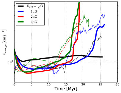
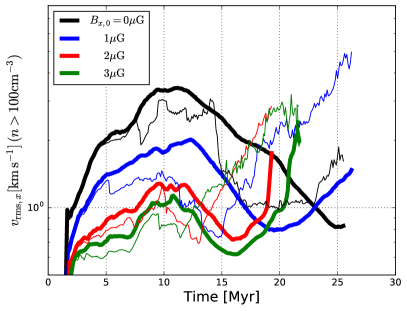
Figure 3: Left: Evolution of the transverse velocity dispersion (in the plane perpendicular to the inflows) for all the gas in the “central box” (a cylinder of length and diameter equal to 80 pc, centered at the plane where the inflows collide; see Sec. 4) for the 4 simulations. The thick and thin lines correspond to the velocity dispersion weighted by volume and density, respectively. Right: Evolution of the longitudinal velocity dispersion in the same box, considering only the dense gas ($n>100\,{\rm cm}^{-3}$) in order to avoid picking up the inflows. The meaning of the thick and thin lines is the same as in the left panel. It is seen that both the volume- and density weighted dispersion increases for progressively smaller magnetic field strength, being almost 4 times larger in the non-magnetic case than in the case with $B=3\,\mu$G. The strong increase of the longitudinal (and transverse) velocity dispersion in the magnetic runs B1, B2 and B3 toward the final stages of the simulations is due to the gravitational contraction. This behavior is most evident in the density–weighted dispersion (thin lines).

Interestingly, both the transverse and longitudinal density–weighted velocity dispersions shown in Fig. 3 (thin lines) exhibit a sudden increase after $t\sim 12\,{\rm Myr}$, which we attribute to the gravitational collapse (in agreement with, e.g., Vázquez-Semadeni et al., 2007). Note that the clouds with higher magnetic field strength exhibit this behavior earlier since these clouds accumulate mass faster (see Fig. 7) and thus become gravitationally supercritical earlier.

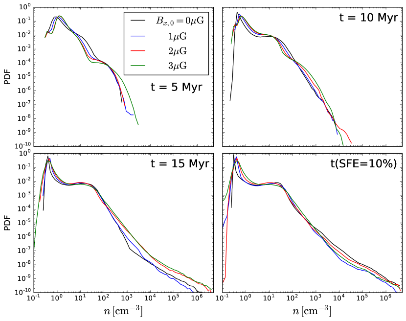
Figure 4: Volume-weighted density PDF for the different models at $t=5$, $10$, and $15\,{\rm Myr}$ for the central box (of 80 pc per side). The lower right panel shows the density PDFs for all the models at the time at which the star formation efficiency is 10% ($t=25.0$, $19.8$, $16.6$, and $15.5\,{\rm Myr}$, corresponding to models B0, B1, B2 and B3, respectively).

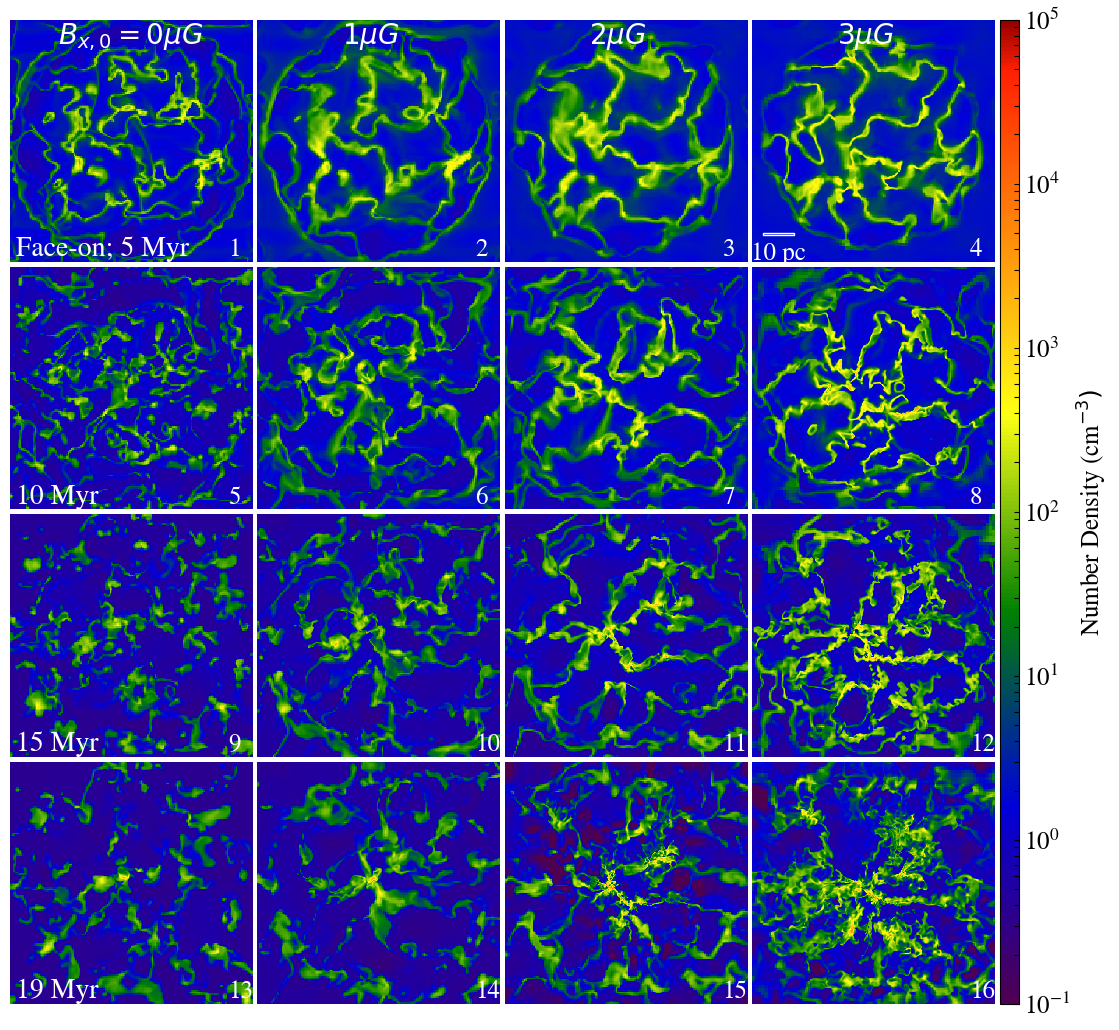
Figure 5: Face-on slices of the number density for the “central clouds” at $t=5$, $10$, $15$, and $19\,{\rm Myr}$. As in Fig. 4, the different columns represent the models B0, B1, B2, and B3 and the box size is $80\,{\rm pc}$ per side (see the scale in panel 4). Note that clumps and filaments are preferably green ($10\,{\rm cm}^{-3}\lesssim n\lesssim 10^{2}{\rm cm}^{-3}$) in models B0 and B1, whereas they tend to be yellow ($10^{2}\,{\rm cm}^{-3}\lesssim n\lesssim 10^{3}{\rm cm}^{-3}$) for B2 and B3 models.

4.3 Evolution of the Density PDFs

The different evolution of the clouds caused by the difference in the background magnetic field is also reflected on their volume-weighted density PDFs (see Fig. 4). Although in general the PDFs of all four runs exhibit the bimodal shape characteristic of thermally bistable flows (e.g., Vazquez-Semadeni et al., 2000; Audit & Hennebelle, 2005; Gazol et al., 2005), with maxima at $n\sim 0.3\,{\rm cm}^{-3}$ and $30\,{\rm cm}^{-3}$, these features do not develop clearly until $t\sim 10$ Myr. At earlier times ($t\sim 5$ Myr), as mentioned in Sec. 4.2, a prominent feature corresponding to the early filament formation is present at $n\sim 100\,{\rm cm}^{-3}$, although it is more pronounced in cases with stronger magnetic fields, indicating that the stronger level of turbulence generated in the cases with weaker fields partially disrupts the filaments, or prevents their formation.

At later times, the increasing dominance of gravity leaves its imprint on the PDFs. Interestingly, at $15\,{\rm Myr}$ (see lower left panel of Fig. 4), the density PDF for all runs exhibits two power low tails at high densities, a feature recently reported in observations toward giant molecular clouds (GMCs; see e.g., Schneider et al., 2015). As time progresses, the dense gas fraction increases, the increase being faster in the more strongly magnetized cases (see this trend in the upper right and lower left panels of Fig. 4), an effect that is directly reflected in a faster increase of the SFR (see Section 4.5). However, at the time at which the star formation efficiency (SFE; eq. [5]) is $10\%$ in each run (at $t=25.0$, $19.8$, $16.6$, and $15.5\,{\rm Myr}$ for the models B0, B1, B2 and B3, respectively), the trend is reversed because at weaker field strengths the collapse takes longer to initiate, since the cloud was initially more dispersed. Nevertheless, at later times the collapse does proceed more freely for weaker field strength. This is reflected in the fact that run B0 takes 10 Myr more than run B3 to reach an SFE of 10%, but by the time it does so, its star formation rate (SFR) is increasing faster (cf. Sec. 4.5).

Finally, note that, in all runs, we terminate the inflows at $t\sim 15$ Myr, and therefore the clouds are no longer fed by the diffuse gas inflows after this time. Thus, from this time on, the volume occupied by the dense gas ($n>100\,{\rm cm}^{-3}$) decreases while its mean density increases (Fig. 6), which is a clear sign of global collapse, even for the more diffuse and less compact clouds (models B0 and B1).

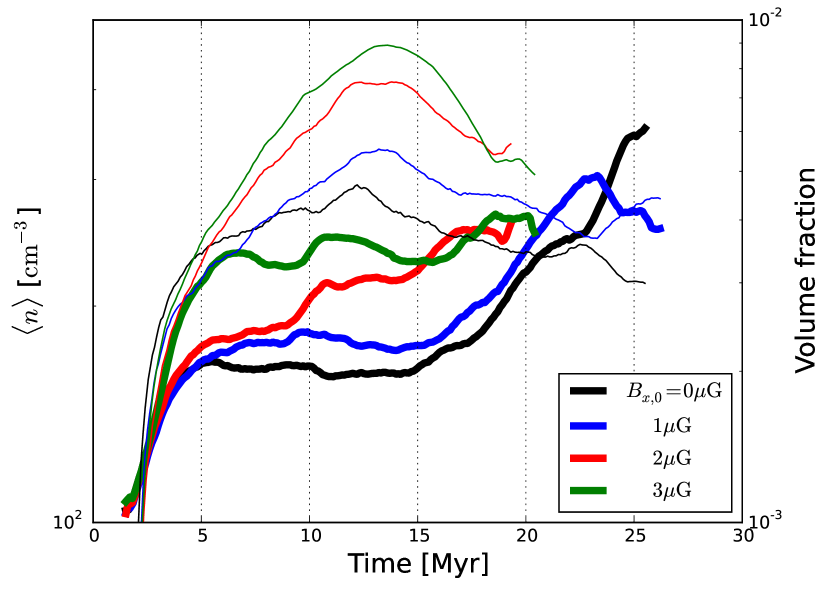
Figure 6: Evolution of the mean number density of dense gas ($n>100\,{\rm cm}^{-3}$; thick lines) of the “central cloud” in the simulations with $B_{x,0}=0$, $1$, $2$, and $3\,\mu{\rm G}$. The thin lines represent the volume fraction of the dense gas in the central boxes.

4.4 Cloud mass

Figure 7 shows the effect of increasing the magnetic field strength on the cloud mass. It is seen that the clouds in the models with higher magnetic field strength accumulate their mass faster and reach higher maximum masses, by up to a factor of $3$ (compare, for instance, models B0 and B3). This result is in accordance with simulations with a similar setup by Heitsch et al. (2009) (see their Figure 2), but without self-gravity. This suggests that the stronger turbulence in the weakly magnetized cases counteracts the transition from the warm to the cold phase induced by TI, effectively reducing the amount of cold, dense gas produced.

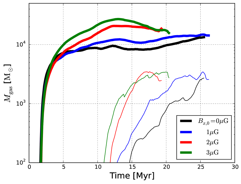
Figure 7: Evolution of the dense gas mass with $n>100\,{\rm cm}^{-3}$ (thick lines) and $n>10^{4}\,{\rm cm}^{-3}$ (thin lines) of the “central cloud” for the simulations with $B_{x,0}=0$, $1$, $2$, and $3\,\mu{\rm G}$. Simulations with higher (initial) magnetic field strength accumulate their mass faster and produce clouds with higher maximum masses.

4.5 The Star Formation Rate and Efficiency

The star formation activity in the simulations exhibits strong intermittency in both space and time. Because the clouds are contracting gravitationally, they are becoming denser on average. As shown by Zamora-Avilés et al. (2012), this implies that quantities such as the SFE and SFR are naturally time-dependent, and increase in time until feedback (not included in the present study) begins to destroy the clouds.

As in previous works (e.g., Vázquez-Semadeni et al., 2007; Vázquez-Semadeni et al., 2010; Zamora-Avilés et al., 2012; Colín et al., 2013; Zamora-Avilés & Vázquez-Semadeni, 2014), we define the instantaneous SFE as

$${\rm SFE}(t)=\frac{M_{\rm S}(t)}{M_{\rm C}(t)+M_{\rm S}(t)},$$ (5)

where $M_{\rm C}$ is the cloud mass (specifically, the gas mass at $n>100\,{\rm cm}^{-3}$), and $M_{\rm S}$ is the total mass in stars, which we take as the total mass in sinks, $M_{\rm sinks}$.

We estimate the SFR as the time derivative of the total sink mass, $dM_{\rm sinks}(t)/dt$ (which is calculated by dividing the difference in the total sink mass in a time step by the duration of the step). This accounts for both the mass collapsed onto new sinks and the mass accreted onto the existing ones. Figures 8 and 9 show the time evolution of the SFR and SFE for the various simulations with different initial strengths of magnetic field. In general, it is seen that both the SFE and the SFR increase monotonically in time until the end of the simulations. This is due to the inherent increase of the SFR caused by the collapse of the clouds, and to the neglect of stellar feedback (cf. Sec. 3.2), which has been shown previously to partially or completely suppress the SF activity in the clouds, depending on their mass (and possibly geometry) (e.g., Vázquez-Semadeni et al., 2010; Dale et al., 2012, 2013; Colín et al., 2013). Therefore, in the present simulations, there is no agent that prevents the continued increase of the SFR. However, this allows us to investigate the effects of varying the magnetic field alone.

In this context, several points are worth noting in Figs. 8 and 9. First, it is seen that the onset of SF is delayed by larger amounts at weaker values of the magnetic field strength, although it is nearly simultaneous for runs B1 and B0. Morever, while run B2 and B3 start forming sinks before the inflows end ($t\sim 15$ Myr), runs B0 and B1 only begin forming sinks when the inflows have ended. Second, run B0 exhibits an initial period of nearly 2 Myr during which the SFR decreases, but after that time, its SFR begins increasing. A similar initial decrease of the SFR is observed in run B1, although its duration is shorter, $\sim 1$ Myr. Third, it is seen that, once the SFRs of all simulations are increasing, the SFR increase rate of run B0 is larger than that of the magnetic runs (see Section 4.3). Finally, note that the SFE (as well as the SFR) is much higher than that typically observed in GMCs ($\sim 2$%, e.g., Myers et al., 1986) due to the absence of stellar feedback (see Secs. 3.2 and 5.3.1). However, this is not a problem because here we are not attempting to reproduce actual observed SFEs, but rather to isolate the effects of varying the magnetic field on the SFR and the SFE.

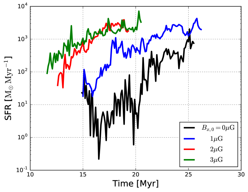
Figure 8: Evolution of the SFR. The onset of SF is seen to be delayed as the background magnetic field strength is decreased, although it is nearly simultaneous for runs B1 and B0.

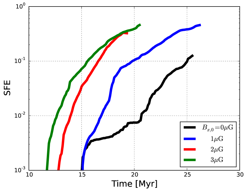
Figure 9: Evolution of the star formation efficiency (SFE; see eq. 5) for the four simulations. Note that, because stellar feedback is not included (cf. Sec. 3.2), the SFE is seen to reach values larger than observed values for whole GMCs (see e.g., Vázquez-Semadeni et al., 2010; Colín et al., 2013; Dale et al., 2013; Walch & Naab, 2015)).

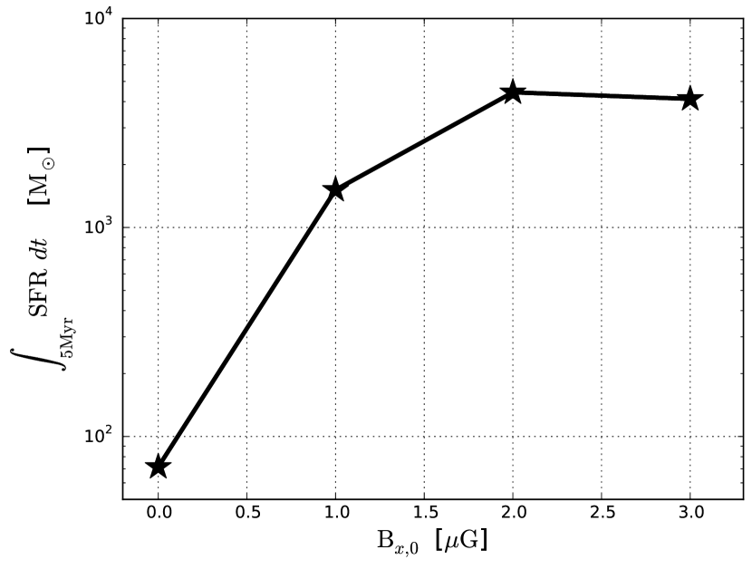
Figure 10: Total mass in sinks $5\,{\rm Myr}$ after the onset of star formation (i.e., the SFR integrated during this time interval) for all runs. Note that, on average, the star formation activity increases with increasing magnetic field strength.

5 Discussion

5.1 Comparison with previous work

The effect of the magnetic field strength and orientation in the assembly and star-forming activity of MCs has been addressed by several studies in the past (see e.g., Passot et al., 1995; Hennebelle & Pérault, 2000; Ballesteros-Paredes & Mac Low, 2002; Heitsch et al., 2009; Banerjee et al., 2009; Vázquez-Semadeni et al., 2011; Hill et al., 2012; Walch et al., 2015; Körtgen & Banerjee, 2015). In particular, Passot et al. (1995) showed that the dependence of the SFR on the magnetic field strength is highly non-monotonic. In particular, at intermediate magnetic field strengths, an increase of the uniform background field tends to suppress shearing motions in the medium that disrupt clouds, thereby promoting the growth of density fluctuations (see also Ballesteros-Paredes & Mac Low, 2002). In our case, the shearing motions are caused by the NTSI, and their inhibition by the magnetic field leads to the formation of more massive clouds (cf. Sec. 4.4 and Fig. 7) and therefore a larger total stellar mass (Fig. 10). The latter shows the total mass in sinks 5 Myr after the onset of star formation in all runs, and can be compared to Figure 8 in Passot et al. (1995). Note that although the setup of those authors was very different from ours (as well as the numerical techniques), and the shearing in the study of those authors was due to differential galactic rotation, not the NTSI, the effect of magnetic fields on reducing shearing motions that inhibit contraction is similar.

In addition, our results are consistent with those of Heitsch et al. (2009), who also studied the problem of cloud formation by converging flows in the case where the magnetic fields are aligned with the flows, although they considered only the role of the magnetic field in the process of cloud formation, excluding self-gravity (see also Heitsch et al., 2007). Those authors found that increasing the magnetic field strength tends to weaken (or even suppress) the NTSI, which results in clouds with reduced levels of turbulence, larger masses and smaller sizes, in agreement with our results (see Fig. 7).

Our findings can also be compared to those of Carroll-Nellenback et al. (2014, hereafter CN+14), who used a setup similar to ours, but not including the magnetic field. Interestingly, rather than investigating the effect of variations of the intensity of the background magnetic field, those authors were concerned with the effect of pre-existing clumpiness in the colliding flows. They found that clouds formed by clumpy inflows are in general more turbulent and have lower total mass (gas + sinks) as well as fewer but more massive sink particles. Therefore, the cloud formed by clumpy inflows in that study is similar to the clouds formed at lower field strengths in our case, although for a different reason: in the case of CN+14, the cloud is scattered because the clumpiness of the incoming flows reduces the amount of mass that collides directly against material from the opposing inflow, thus reducing the dissipation of the kinetic energy of the inflows. Instead, in our case, the presence of progressively stronger magnetic fields causes a suppression of the NTSI, reducing the generation of turbulence in the cloud, as well as the “bounce” (i.e., the rebound of the dense layer because of an increase in its internal turbulent ram pressure; see Fig. 2) that results from the development of the instability (see Sec. 4.2).

It is worth noting that we use a very similar setup as that in the works presented by Banerjee et al. (2009, hereafter B+09, VS+11, and KB15, respectively); Vázquez-Semadeni et al. (2011, hereafter B+09, VS+11, and KB15, respectively); Körtgen & Banerjee (2015, hereafter B+09, VS+11, and KB15, respectively), although with different parameters in the initial conditions as shown in Table 1. Our model B2 ($\mu/\mu_{\rm crit}=2.38$) can be compared with the simulation presented by Banerjee et al. (2009) ($\mu/\mu_{\rm crit}\approx 2.9$). Comparing the SFE at the end of the simulations (see their Fig. 13 and Fig. 5 in this work) we find quite similar values in both models (around $\sim$40-50%).

On the other hand, VS+11 present simulations with $\mu/\mu_{\rm crit}\approx 1.36,0.91$, and 0.68, so we can compare their magnetically supercritical simulation (B2-AD model) with our model B3 ($\mu/\mu_{\rm crit}\approx 1.59$). Their SFE saturates again at $\sim 40$%, in agreement with our B3 model (compare the lower-right panel of their Fig. 5 to our Fig. 9). Note that the evolving time scales are different in the mentioned works since the inflow parameters are different. It also should be noticed, however, that most of the inflow parameters used in this work are different to those used in Banerjee et al. (2009) and VS+11 (see Table 1) suggesting that the dominant parameter controlling the turbulence level and the SF activity itself is the “magnetic criticality” (through the $\mu/\mu_{\rm crit}$ ratio), although more research is needed in this regard (particularly an uniform parameter study).

Lastly, KB15 only studied magnetically subcritical clouds and so our models cannot be compared directly, but can be considered complementary to our work instead. Interestingly, these authors find that in sub-critical clouds (specifically in their models with $\mu/\mu_{\rm crit}\approx$ 0.59 and 0.47 listed in Table 1) the NTSI may be suppressed since the $\beta_{\rm ram}$ parameter is less than 1 (following the trend shown in Fig. 2; see also Fig. 12 in KB15).

5.2 Test of the refinement criterion

Our constant-mass refinement criterion does not fulfill the Truelove criterion (Truelove et al., 1997) for prevention of spurious fragmentation. This criterion requires the resolution to scale linearly with the Jeans length $L_{\rm J}$ (i.e., as $\rho^{-1/2}$, assuming constant temperature; see eq. [2]). Instead, with our criterion, the resolution scales as $\rho^{-1/3}$, or equivalently, as $L_{\rm J}^{2/3}$, implying that the Jeans length is increasingly more poorly resolved as the density increases, and therefore, some artificial fragmentation may be expected.

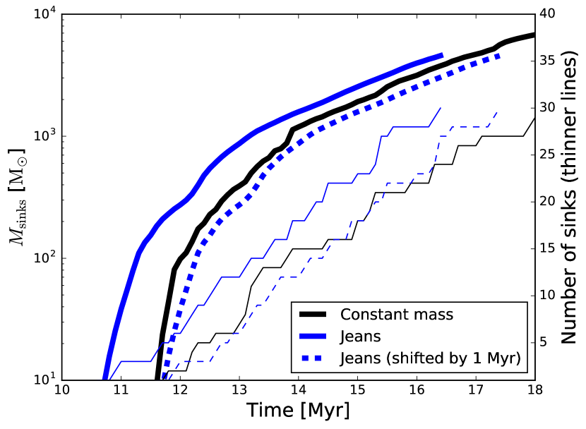
Figure 11: Time evolution of the number (thin lines) and the total mass in sinks (thick lines) for runs B3 (which uses the constant mass refinement criterion) and B3J (Jeans criterion). Note that both the number and the total mass in sinks are very similar when we consider the curves for the run B3J shifted by $1\,Myr$ (discontinuous lines).

In order to quantify this effect, we performed an additional simulation, labeled B3J, which is identical to run B3 except for the refinement criterion used. For run B3J we use the Jeans criterion and we resolve the Jeans length (eq. 2) by at least 10 grid cells in order to fulfill the Truelove criterion ; i.e., the condition $\lambda_{\rm J}\geq 10\times\Delta x$ is satisfied in every cell. At the higher level of refinement, this condition imposes a density threshold for sink formation of $\rho_{\rm thr}=7.1\times 10^{-20}\,{\rm g\leavevmode\nobreak\ cm}^{-3}$($=1.8\times 10^{4}\,{\rm cm}^{-3}$), which is two orders of magnitude lower than the threshold used in the constant-mass criterion. Thus, using the Jeans criterion instead of the constant-mass one, we expect an earlier onset of star formation. Figure 11 shows the evolution of the number of sink particles (thin continuous lines; right $y$-label) and the total mass in them (thick continuous lines). It can be seen that both quantities are very close for the two simulations, and that the effect of choosing the Jeans criterion over the constant mass criterion is just to delay the onset of star formation by $10$%, as can be appreciated from the dashed lines in the same figure, which were shifted by 1 Myr just to illustrate this difference. Therefore, the effect of the refinement criterion on our results is just an offset in the onset of star formation. For instance, a shift of 1 Myr puts run B3 in the same temporal starting point as run B2 in Fig. 8. However, we expect the rest of the cloud properties to remain qualitatively the same.

5.3 Limitations

5.3.1 Neglected processes

One of the most notable omissions in our simulations is that of stellar feedback. In particular, the ionizing radiation from massive stars is generally considered to be the dominant mechanism of stellar energy injection into GMCs (Matzner, 2002), although its effect may be mostly the dispersal of the clouds rather than maintaining them in a near-equilibrium state and reducing both the SFR and the SFE (Vázquez-Semadeni et al., 2010; Zamora-Avilés et al., 2012; Dale et al., 2012, 2013; Colín et al., 2013). Moreover, after a few Myr, SN explosions are expected to begin occurring, contributing to further cloud dispersal, although the effect may not be stronger than that of ionizing radiation (e.g., Walch & Naab, 2015; Iffrig & Hennebelle, 2015; Körtgen et al., 2016).

Nevertheless, as mentioned above, in this paper we have not been concerned so much about generating a realistic model of MCs at all times in their evolution, but rather in performing a series of numerical experiments assessing the effect of the uniform magnetic field strength in setting up the initial conditions of the clouds. For this purpose, our numerical simulations are appropriate.

6 Summary and Conclusions

In this paper, we have presented four MHD simulations aimed at studying the evolution of MCs formed by diffuse converging flows in the presence of magnetic fields, in order to investigate the effect of the latter on the development of the initial conditions of the nascent clouds and their early star formation activity. We have considered four otherwise identical numerical models except for the initial magnetic field strength, for which we have considered the values $0$, $1$, $2$, and $3\,\mu{\rm G}$ (models B0, B1, B2, and B3, respectively), corresponding to magnetically supercritical configurations in all cases. The field is initially aligned with the flows. The latter is not a restrictive condition, however, since it has been shown that, when the flows are oblique to the magnetic field and have sufficiently high Mach numbers (depending on the field strength), the flows are reoriented to proceed along the magnetic field (Hennebelle & Pérault, 2000). Therefore, whenever the flows manage to collide, they will do so aligned with the field.

In the initial phase of cloud formation, our simulations show that, in agreement with the non-self-gravitating results from Heitsch et al. (2009), the presence of a magnetic field aligned with the inflows tends to suppress the NTSI, causing the clouds to be more compact, denser, and less turbulent. In the presence of self-gravity, this leads to an earlier global collapse of the clouds, and to an enhanced early star-formation activity. Instead, more weakly magnetized, or fully non-magnetic cases produce more dispersed and more turbulent clouds, that initially expand in a rebound from the initial collision, and only later begin to collapse. However, when they do so, their SFRs increase more rapidly, because the collapse is then unimpeded by the magnetic field.

Moreover, the non-magnetic simulation, run B0, and that with the weakest magnetic field (B1), do not start their collapse until the inflows are terminated. Note, however, that this does not necessarily imply that the turbulence generated by the inflows is sufficient to support the clouds, since it is possible that, if the inflows were maintained for longer times, the clouds could gain enough mass to begin their collapse (further study is necessary in order to address this issue). Nevertheless, because the accepted value of the mean magnetic field strength in the ISM is comparable to that considered in our more strongly magnetized cases (runs B2 and B3; Beck et al., 1996), our results reinforce the notion that the turbulence produced by the stream collision in the nascent clouds is not enough to support them against their self-gravity (Vázquez-Semadeni et al., 2007), and therefore engage in global gravitational contraction soon after they are assembled.

This conclusion is further reinforced by the fact that the clouds in runs B0 and B1, which are supported by turbulence in their initial stages, do not begin forming stars until after the inflows, and therefore the turbulence driving, are terminated, and the clouds engage in global gravitational contraction. This suggests that star-forming GMCs are in general in a state of global collapse.

References

- Audit & Hennebelle (2005) Audit E., Hennebelle P., 2005, A& A, 433, 1
- Ballesteros-Paredes & Mac Low (2002) Ballesteros-Paredes J., Mac Low M.-M., 2002, ApJ, 570, 734
- Ballesteros-Paredes et al. (1999) Ballesteros-Paredes J., Hartmann L., Vázquez-Semadeni E., 1999, ApJ, 527, 285
- Banerjee et al. (2009) Banerjee R., Vázquez-Semadeni E., Hennebelle P., Klessen R. S., 2009, MNRAS, 398, 1082
- Beck et al. (1996) Beck R., Brandenburg A., Moss D., Shukurov A., Sokoloff D., 1996, ARA&A, 34, 155
- Bouchut et al. (2007) Bouchut F., Klingenberg C., Waagan K., 2007, Numerische Mathematik
- Bouchut et al. (2010) Bouchut F., Klingenberg C., Waagan K., 2010, Numerische Mathematik
- Carroll-Nellenback et al. (2014) Carroll-Nellenback J. J., Frank A., Heitsch F., 2014, ApJ, 790, 37
- Chandrasekhar (1961) Chandrasekhar S., 1961, Hydrodynamic and hydromagnetic stability
- Colín et al. (2013) Colín P., Vázquez-Semadeni E., Gómez G. C., 2013, MNRAS, 435, 1701
- Crutcher et al. (2010) Crutcher R. M., Wandelt B., Heiles C., Falgarone E., Troland T. H., 2010, ApJ, 725, 466
- Dale et al. (2012) Dale J. E., Ercolano B., Bonnell I. A., 2012, MNRAS, 424, 377
- Dale et al. (2013) Dale J. E., Ercolano B., Bonnell I. A., 2013, MNRAS, 430, 234
- Elmegreen (1994) Elmegreen B. G., 1994, ApJ, 433, 39
- Federrath et al. (2010) Federrath C., Banerjee R., Clark P. C., Klessen R. S., 2010, ApJ, 713, 269
- Field (1965) Field G. B., 1965, ApJ, 142, 531
- Folini & Walder (2006) Folini D., Walder R., 2006, A& A, 459, 1
- Fryxell et al. (2000) Fryxell B., et al., 2000, ApJS, 131, 273
- Gazol et al. (2005) Gazol A., Vázquez-Semadeni E., Kim J., 2005, ApJ, 630, 911
- Gómez & Vázquez-Semadeni (2014) Gómez G. C., Vázquez-Semadeni E., 2014, ApJ, 791, 124
- Hartmann et al. (2001) Hartmann L., Ballesteros-Paredes J., Bergin E. A., 2001, ApJ, 562, 852
- Heitsch & Hartmann (2008) Heitsch F., Hartmann L., 2008, ApJ, 689, 290
- Heitsch & Hartmann (2014) Heitsch F., Hartmann L., 2014, MNRAS, 443, 230
- Heitsch et al. (2005) Heitsch F., Burkert A., Hartmann L. W., Slyz A. D., Devriendt J. E. G., 2005, ApJL, 633, L113
- Heitsch et al. (2006) Heitsch F., Slyz A. D., Devriendt J. E. G., Hartmann L. W., Burkert A., 2006, ApJ, 648, 1052
- Heitsch et al. (2007) Heitsch F., Slyz A. D., Devriendt J. E. G., Hartmann L. W., Burkert A., 2007, ApJ, 665, 445
- Heitsch et al. (2008) Heitsch F., Hartmann L. W., Burkert A., 2008, ApJ, 683, 786
- Heitsch et al. (2009) Heitsch F., Stone J. M., Hartmann L. W., 2009, ApJ, 695, 248
- Hennebelle (2013) Hennebelle P., 2013, A& A, 556, A153
- Hennebelle & Pérault (1999) Hennebelle P., Pérault M., 1999, A& A, 351, 309
- Hennebelle & Pérault (2000) Hennebelle P., Pérault M., 2000, A& A, 359, 1124
- Hill et al. (2012) Hill A. S., Joung M. R., Mac Low M.-M., Benjamin R. A., Haffner L. M., Klingenberg C., Waagan K., 2012, ApJ, 750, 104
- Hoyle (1953) Hoyle F., 1953, ApJ, 118, 513
- Hunter et al. (1986) Hunter Jr. J. H., Sandford II M. T., Whitaker R. W., Klein R. I., 1986, ApJ, 305, 309
- Iffrig & Hennebelle (2015) Iffrig O., Hennebelle P., 2015, A& A, 576, A95
- Inoue & Inutsuka (2008) Inoue T., Inutsuka S.-i., 2008, ApJ, 687, 303
- Inoue & Inutsuka (2009) Inoue T., Inutsuka S.-i., 2009, ApJ, 704, 161
- Inoue & Inutsuka (2012) Inoue T., Inutsuka S.-i., 2012, ApJ, 759, 35
- Inutsuka et al. (2015) Inutsuka S.-i., Inoue T., Iwasaki K., Hosokawa T., 2015, A& A, 580, A49
- Jeans (1902) Jeans J. H., 1902, Philosophical Transactions of the Royal Society of London Series A, 199, 1
- Kim et al. (2003) Kim W.-T., Ostriker E. C., Stone J. M., 2003, ApJ, 599, 1157
- Körtgen & Banerjee (2015) Körtgen B., Banerjee R., 2015, MNRAS, 451, 3340
- Körtgen et al. (2016) Körtgen B., Seifried D., Banerjee R., Vázquez-Semadeni E., Zamora-Avilés M., 2016, MNRAS, 459, 3460
- Koyama & Inutsuka (2000) Koyama H., Inutsuka S. I., 2000, ApJ, 532, 980
- Koyama & Inutsuka (2002) Koyama H., Inutsuka S. I., 2002, ApJL, 564, L97
- Lazarian (2014) Lazarian A., 2014, SSRv, 181, 1
- Matzner (2002) Matzner C. D., 2002, ApJ, 566, 302
- Myers et al. (1986) Myers P. C., Dame T. M., Thaddeus P., Cohen R. S., Silverberg R. F., Dwek E., Hauser M. G., 1986, ApJ, 301, 398
- Nakano & Nakamura (1978) Nakano T., Nakamura T., 1978, PASJ, 30, 671
- Ostriker et al. (2001) Ostriker E. C., Stone J. M., Gammie C. F., 2001, ApJ, 546, 980
- Passot et al. (1995) Passot T., Vazquez-Semadeni E., Pouquet A., 1995, ApJ, 455, 536
- Pon et al. (2011) Pon A., Johnstone D., Heitsch F., 2011, ApJ, 740, 88
- Sánchez-Salcedo et al. (2002) Sánchez-Salcedo F. J., Vázquez-Semadeni E., Gazol A., 2002, ApJ, 577, 768
- Schneider et al. (2015) Schneider N., et al., 2015, MNRAS, 453, L41
- Truelove et al. (1997) Truelove J. K., Klein R. I., McKee C. F., Holliman II J. H., Howell L. H., Greenough J. A., 1997, ApJL, 489, L179
- Turk et al. (2011) Turk M. J., Smith B. D., Oishi J. S., Skory S., Skillman S. W., Abel T., Norman M. L., 2011, ApJS, 192, 9
- Vázquez-Semadeni (2015) Vázquez-Semadeni E., 2015, in Lazarian A., de Gouveia Dal Pino E. M., Melioli C., eds, Astrophysics and Space Science Library Vol. 407, Magnetic Fields in Diffuse Media. p. 401 (arXiv:1208.4132), doi:10.1007/978-3-662-44625-6˙14