Bayesian dimensionality reduction with PCA using penalized semi-integrated likelihood

Abstract

We discuss the problem of estimating the number of principal components in Principal Components Analysis (PCA). Despite of the importance of the problem and the multitude of solutions proposed in the literature, it comes as a surprise that there does not exist a coherent asymptotic framework which would justify different approaches depending on the actual size of the data set. In this paper we address this issue by presenting an approximate Bayesian approach based on Laplace approximation and introducing a general method for building the model selection criteria, called PEnalized SEmi-integrated Likelihood (PESEL). Our general framework encompasses a variety of existing approaches based on probabilistic models, like e.g. Bayesian Information Criterion for the Probabilistic PCA (PPCA), and allows for construction of new criteria, depending on the size of the data set at hand and additional prior information. Specifically, we apply PESEL to derive two new criteria for data sets where the number of variables substantially exceeds the number of observations, which is out of the scope of currently existing approaches. We also report results of extensive simulation studies and real data analysis, which illustrate good properties of our proposed criteria as compared to the state-of-the-art methods and very recent proposals. Specifically, these simulations show that PESEL based criteria can be quite robust against deviations from the probabilistic model assumptions. Selected PESEL based criteria for the estimation of the number of principal components are implemented in R package varclust, which is available on github (https://github.com/psobczyk/varclust).

^a Faculty of Pure and Applied Mathematics, Wrocław University of Science and Technology, Wroclaw, Poland
^b Institute of Mathematics, University of Wrocław, Wroclaw, Poland
^c INRIA, Paris, France
^d Department of Applied Mathematics, Agrocampus Ouest, Rennes, France

Keywords: laplace approximation, bayesian model selection

1 Introduction

Principal Component Analysis (PCA) [Pearson, 1901] is a widely used technique for dimensionality reduction. It is applied in many fields as a way to visualize multidimensional data, which is projected onto a number of orthogonal directions in a low dimensional space. Researcher can examine this representation to get intuition about the data structure and conjecture a hypothesis, that would be further investigated. We treat first components in PCA as signal, and the rest of components as noise. In such exploratory analysis, it is often redundant to have a tool for precise choice of the number of non-noise components. But there are many situations where accuracy of this estimation is important. For example in projective clustering (see e.g. [Agarwal and Mustafa, 2004]), where data is clustered along various linear subspaces, an incorrect estimation of subspaces dimensions may lead to the choice of wrong number of clusters and incorrect segmentation. Other example is the important problem of missing values in PCA, where inaccurate estimation of the number of components may lead to overfitting (see [Josse et al., 2009], [Ilin et al., 2010], [Josse et al., 2011]).

Let $\mathbf{X}=[x_{ij}]_{n\times p}$ be high-dimensional data, where $n$ is the number of observations and $p$ is the number of variables. Consider the fixed effect model for PCA:

$$\mathbf{X}-\bm{\mu}_{n\times p}=\mathbf{M}+E,$$ (1)

where $\bm{\mu}$ is of rank one, $\mathbf{M}$ is assumed to be of low rank $k\leq\min(n,p)$ and $E=[\epsilon_{i,j}]_{n\times p}$ is a matrix of i.i.d. errors, $\epsilon_{i,j}\sim\mathcal{N}(0,\sigma^{2})$. Equivalently we may write model  (1) as in  Caussinus [1986]:

$$\mathbf{X}-\bm{\mu}_{n\times p}=\mathbf{T}\mathbf{W}^{T}+E,$$ (2)

where $\mathbf{T}=[t_{i,l}]_{n\times k}$ is a matrix whose columns contain factors spanning the data, and $\mathbf{W}=[w_{i,l}]_{p\times k}$ is a matrix of coefficients.

Given the number of components $k$, maximum likelihood estimators for $\mathbf{T}$ and $\mathbf{W}$ are obtained by performing SVD decomposition of $\mathbf{X}-\bm{\mu}$ truncated at the order $k$ (see for example [Caussinus, 1986],  [Allen et al., 2014]).

In Jolliffe [2002] three types of methods for choosing the number of factors are distinguished. First are ad-hoc rules such as a scree test [D’agostino and Russell, 2005] or a rule of thumb that chooses the smallest number of factors which jointly explain e.g. 90% of variance of data. Although these methods are usually fast and easy to implement, they are difficult to use in automatic way, since in high-dimensional data it is common that few first components explain a lot of variance even if data is entirely random [Husson et al., 2010]. Therefore these heuristic approaches are rather useless when PCA is used without supervision.

Second type are techniques that view the problem in a more systematic way but are not based on any probabilistic assumptions. Among them are bootstrap and permutation methods (see [Jackson, 1993]) and cross-validation (see [Owen and Perry, 2009],  [Josse and Husson, 2012]). Finally there exists a group of methods based on asymptotic approximation for a specific probabilistic model, which we discuss in more detail in Section 2.

Despite the fact that there exist various probabilistic approaches for choosing the number of principal components (e.g. [Tipping and Bishop, 1999]), there seems to be no coherent framework that would unify them. Additionally, according to our knowledge, there exist no proper criteria to deal with the situation when the number of variables is substantially larger than the number of observations. In this paper we address these issues by introducing a novel approximate Bayesian framework for model selection. As existing full Bayesian methods (see e.g. [Hoff, 2007]) are computationally expensive and require specifying many prior distributions, we suggest instead to use approximated formula for the posterior probability. Our focus is on Bayesian Information Criterion, which is based on the Laplace approximation. This approach requires the number of degrees of freedom in the model to be independent of the number of observations. As this is not satisfied by (2), we need to analytically integrate out some of the priors. First strategy relies on integrating out the prior on $\mathbf{T}$, which reduces number of parameters in the model, so it no longer depends on $n$. Hence we get PESEL (PEnalized SEmi-integrated Likelihood) valid for $n\to\infty$. Second strategy is integrating out the prior on $\mathbf{W}$, which gives criterion valid for $p\to\infty$.

Thus, it is useful for the sequel to express (2) as a model for either rows or columns of the matrix $\mathbf{X}$, for which we shall use notation $x_{i\raisebox{-0.75346pt}{\scalebox{1.5}{$\cdot$}}}$ and $x_{\raisebox{-0.75346pt}{\scalebox{1.5}{$\cdot$}}j}$ respectively.

$$\begin{split}\mathbf{x}_{i\raisebox{-0.75346pt}{\scalebox{1.5}{$\cdot$}}}-\bm{\mu}_{i\raisebox{-0.75346pt}{\scalebox{1.5}{$\cdot$}}}&=\sum_{l=1}^{k}t_{i,l}\,\mathbf{w}_{\raisebox{-0.75346pt}{\scalebox{1.5}{$\cdot$}}l}+\epsilon_{i\raisebox{-0.75346pt}{\scalebox{1.5}{$\cdot$}}}=\mathbf{t}_{i\raisebox{-0.75346pt}{\scalebox{1.5}{$\cdot$}}}\,\mathbf{W}^{T}+\epsilon_{i\raisebox{-0.75346pt}{\scalebox{1.5}{$\cdot$}}},\;\;\;i=1,\dots,n,\;\;\;\epsilon_{1\raisebox{-0.75346pt}{\scalebox{1.5}{$\cdot$}}},\dots,\epsilon_{n\raisebox{-0.75346pt}{\scalebox{1.5}{$\cdot$}}}\text{ are i.i.d. }\mathcal{N}(0,\mathbf{I}_{p}),\\ \mathbf{x}_{\raisebox{-0.75346pt}{\scalebox{1.5}{$\cdot$}}j}-\bm{\mu}_{\raisebox{-0.75346pt}{\scalebox{1.5}{$\cdot$}}j}&=\sum_{l=1}^{k}w_{j,l}\,\mathbf{t}_{\raisebox{-0.75346pt}{\scalebox{1.5}{$\cdot$}}l}+\epsilon_{\raisebox{-0.75346pt}{\scalebox{1.5}{$\cdot$}}j}=\mathbf{T}\,w^{T}_{j\raisebox{-0.75346pt}{\scalebox{1.5}{$\cdot$}}}+\epsilon_{\raisebox{-0.75346pt}{\scalebox{1.5}{$\cdot$}}j},\;\;\;j=1,\dots,p,\;\;\;\epsilon_{\raisebox{-0.75346pt}{\scalebox{1.5}{$\cdot$}}1},\dots,\epsilon_{\raisebox{-0.75346pt}{\scalebox{1.5}{$\cdot$}}p}\text{ are i.i.d. }\mathcal{N}(0,\mathbf{I}_{n}).\end{split}$$ (3)

Later in Section 2, we shall assume for the model for rows $\mathbf{x}_{i\raisebox{-0.75346pt}{\scalebox{1.5}{$\cdot$}}}$, that $\bm{\mu}=\begin{bmatrix}\mu_{1}&\mu_{2}&\dots&\mu_{p}\\ \vdots&\vdots&\vdots&\vdots\\ \mu_{1}&\mu_{2}&\dots&\mu_{p}\\ \end{bmatrix}$.

Analogously, for the model for columns $\mathbf{x}_{\raisebox{-0.75346pt}{\scalebox{1.5}{$\cdot$}}j}$, we shall assume that $\bm{\mu}=\begin{bmatrix}\mu_{1}&\dots&\mu_{1}\\ \mu_{2}&\dots&\mu_{2}\\ \vdots&\vdots&\vdots\\ \mu_{p}&\dots&\mu_{p}\\ \end{bmatrix}$. In this case vector $[\mu_{1},\dots,\mu_{p}]$ can be interpreted as the mean of the distribution generating variables rather than observations. Such a model is not common, yet it naturally occurs when $p$ is much larger than $n$. In this case all $p$ variables are spanned by just few factors and each new variable is simply defined by the vector of corresponding coefficients, which can be modeled as randomly selected from some underlying distribution.

The outline of the paper is as follows. In Section 2, we introduce the estimation of the number of principal components in a Bayesian setting. In Section 2.2.1 we formulate PESEL for the prior on $\mathbf{T}$ and in Section 2.2.2 we do the same for the prior on $\mathbf{W}$. In Section 3, we assess the performance of the respective selection criteria by computer simulations, in which we compare PESEL to existing and very recents methods. We focus on robustness against deviations from the assumed probabilistic model. In Section 3.4, we present the analysis of the real data, which additionally confirms soundness of the PESEL methodology. Our criteria are implemented in the R package varclust and the code to reproduce all the results available in this paper (including implementation of existing methods for which codes were not provided by the authors) is available at https://github.com/psobczyk/pesel_simulations.

2 Methods based on probabilistic model

To estimate $k$ in a probabilistic setting, we focus on using Bayesian approach and view it as a problem of model selection, where each model $M$ specifies the number of principal components $k$. In general, following maximum a posteriori (MAP) rule, we want to choose a model that is most probable given the data. To do that, we maximize logarithm of the posterior probability

$$\log(P(M|\mathbf{X})) =\log(P(\mathbf{X}|M))+\log(P(M))+C(\mathbf{X})$$

$$=\log\left(\int_{\Theta}p(\mathbf{X}|\theta)\,\pi_{M}(\theta)\,d\theta\right)+\log(P(M))+C(\mathbf{X}),$$

where $P(M)$ is a prior distribution on considered models, $\pi_{M}(\theta)$ is a prior distribution on parameters in a model $M$, and $C(\mathbf{X})$ is a scaling factor that does not depend on $M$. In the reminder of this paper we assume that $P(M)$ is uniform i.e. it does not influence model selection. However; the method can be easily extended for any informative prior distribution on $M$.

In terms of model (2), $\theta=(\bm{\mu},\mathbf{W},\mathbf{T},\sigma)\in\Theta$, and $P(\mathbf{X}|M)$ takes the following form:

$$\log(P(\mathbf{X}|M))=\log\int_{\Theta}p(\mathbf{X}|\bm{\mu},\mathbf{W},\mathbf{T},\sigma)\,\pi_{M}(\bm{\mu},\mathbf{W},\mathbf{T},\sigma)\,d\bm{\mu}\,d\mathbf{W}\,d\mathbf{T}\,d\sigma.$$ (4)

2.1 Full Bayesian approach

There exist several Bayesian methods for estimating the number of principal components in the PCA model. One of them was proposed in Bishop [1999a], who used the following priors in model (2):

$$\mathbf{t}_{i\raisebox{-0.75346pt}{\scalebox{1.5}{$\cdot$}}} \sim\mathcal{N}(0,\mathbf{I}),$$

$$\mathbf{w}_{j\raisebox{-0.75346pt}{\scalebox{1.5}{$\cdot$}}} \sim\mathcal{N}(0,\frac{1}{\alpha_{j}}\mathbf{I}),$$

$$\alpha_{j} \sim\Gamma(a_{\alpha},b_{\alpha}),$$ (5)

$$\frac{1}{\sigma^{2}} \sim\Gamma(c_{\sigma},d_{\sigma}),$$

where $a_{\alpha},b_{\alpha},c_{\sigma},d_{\sigma}$ are model hyperparameters. Rows of $\bm{\mu}$ were estimated with $\bar{\mathbf{x}}=(\overline{\mathbf{x}}_{\cdot 1},\dots,\overline{\mathbf{x}}_{\cdot p})$, where $\overline{\mathbf{x}}_{\cdot j}=\frac{1}{n}\sum^{n}_{i=1}x_{ij}$.

Bishop [1999a] introduces non-discrete “model selection” for PCA, by the means of continuous parameters, that control variability of columns of $\mathbf{W}$. More specifically, large value of $\alpha_{j}$ effectively “switches off” $\mathbf{w}_{j\raisebox{-0.75346pt}{\scalebox{1.5}{$\cdot$}}}$. Bishop [1999a] proposes three computational methods for marginalizing over the posterior on $\mathbf{W}$, including among others Markov Chain Monte Carlo. In the follow up paper, Bishop [1999b] recommends the variational approach, which proves to be the most efficient. This idea was further pursued by Ilin et al. [2010], who propose fast algorithm for variational Bayesian PCA (VBPCA), which is an extension of regular EM algorithm for maximizing likelihood function [Dempster et al., 1977]. However, as mentioned before, VBPCA does not enable direct estimation of the number of PCs.

Another full Bayesian approach was proposed by Hoff [2007], who considered the model (1) with $\bm{\mu}=0$ and priors imposed on components of SVD decomposition of matrix $\mathbf{M}=\mathbf{P}\mathbf{L}\mathbf{Q}^{T}$:

$$\mathbf{P} \sim uniform(\mathcal{S}_{k\times n}),$$

$$\mathbf{Q} \sim uniform(\mathcal{S}_{k\times p}),$$

$$\epsilon_{i\raisebox{-0.75346pt}{\scalebox{1.5}{$\cdot$}}} \sim\mathcal{N}(0,1/\phi),$$

$$l_{i,i} \sim\mathcal{N}(\ell,1/\psi),$$

$$\ell \sim\mathcal{N}(l_{0},v_{0}^{2}),$$ (6)

$$\psi \sim\Gamma(\eta_{0}/2,\eta_{0}\tau_{0}^{2}/2),$$

$$\phi \sim\Gamma(\nu_{0}/2,\nu_{0}\sigma_{0}^{2}/2),$$

where $uniform(\mathcal{S}_{k\times n})$ denotes the uniform distribution on the Stiefel manifold of orthogonal matrices [Chikuse, 2003], $l_{i,i}$ are elements of diagonal matrix $L$ and $(l_{0},v_{0}^{2})$, $(\eta_{0},\tau_{0})$, $(\nu_{0},\sigma_{0})$ are model hyperparameters. To estimate the number of principal components, Hoff [2007] considers the model with $k=p$ and uses the prior on $l_{i,i}$ specified in (6) as a continuous component in the spike and slab prior, with a positive mass at 0. Posterior distributions for parameters are computed with MCMC. Software provided by Hoff [2007] requires $n\geq p$; however, because of symmetry in the model (6), one may transpose the data and then use the method when $p>n$. Due to the complexity of MCMC, implementation is rather slow and does not scale very well. Because even for moderately sized matrices (i.e. $1000\times 100$) generating Markov chain of the length 1000 takes more than two hours, we decided not to include this method in the simulation study.

2.2 PESEL – PEnalized SEmi-integrated Likelihood

Exact calculation of posterior probability, as in Hoff [2007], is computationally expensive and requires specifying all prior distributions. Instead one can perform model selection by approximating integral (4) using Laplace approximation (for more details about Laplace approximation see Appendix A). The integrated likelihood in the fixed effect models (3) for rows takes the form:

$$\log{P(\mathbf{X}|M)} =\log\int_{\Theta}P(\mathbf{X}|\bm{\mu},\mathbf{W},\mathbf{T},\sigma)\,\pi_{M}(\bm{\mu},\mathbf{T},\mathbf{W},\sigma)\,d\bm{\mu}\,d\mathbf{T}\,d\mathbf{W}\,d\sigma$$

$$=\log\int_{\Theta}\Pi_{i=1}^{n}\phi(x_{i\raisebox{-0.75346pt}{\scalebox{1.5}{$\cdot$}}};\bm{\mu}_{i\raisebox{-0.75346pt}{\scalebox{1.5}{$\cdot$}}}+\mathbf{t}_{i\cdot}\mathbf{W}^{T},\sigma^{2}\mathbf{I}_{p})\,\pi_{M}(\bm{\mu},\mathbf{T},\mathbf{W},\sigma)\,d\bm{\mu}\,d\mathbf{T}\,d\mathbf{W}\,d\sigma,$$ (7)

where $\phi(x;\mathbf{m},\bm{\Sigma})$ is a probability density function of normal distribution with mean $\mathbf{m}$ and covariance matrix $\bm{\Sigma}$. It is invalid to apply Laplace approximation directly to the integral (2.2) as number of parameters in this model is proportional to both the number of observations $n$ and the number of variables $p$. This violates Laplace approximation assumption that dimension of the parameter space is constant. Thus, to perform approximation one should reduce dimensionality, for example by integrating out the prior on either $\mathbf{T}$ or $\mathbf{W}$. This choice is determined by asymptotics. For $p\to\infty$ we need to integrate out $\mathbf{W}$ because its number of parameters grows linearly in $p$. Similarly, for $n\to\infty$ $\mathbf{T}$ needs to be integrated out. After integrating out one of the priors, we can apply the Laplace approximation for the resulting semi-integrated likelihood. This yields a new Bayesian criterion for estimating the model dimension, which we call PEnalized SEmi-integrated Likelihood (PESEL).

2.2.1 PESEL for $p$ fixed and $n\to\infty$

If we work in asymptotic regime when $n\to\infty$, then to apply Laplace approximation we need to integrate out $\mathbf{T}$ from (2.2) according to the formula:

$$\log{P(\mathbf{X}|M)} =\log\int SIL(\mathbf{X}|\mu,\mathbf{W},\mathbf{T},\sigma)\pi(\mu,\mathbf{W},\sigma)\,d\mu\,d\mathbf{W}\,d\sigma,$$

where $SIL(\mathbf{X}|\mu,\mathbf{W},\mathbf{T},\sigma):=\int P(\mathbf{X}|\mu,\mathbf{W},\mathbf{T},\sigma)\,\pi(\mathbf{T})\,d\mathbf{T}$ is a semi-integrated likelihood function. In the above $\mu=\bm{\mu}_{i\raisebox{-0.75346pt}{\scalebox{1.5}{$\cdot$}}}=[\mu_{1},\mu_{2},\dots,\mu_{p}]$ are rows of $\bm{\mu}$ from equation (2).

We propose using two forms of PESEL, based on specific priors on rows of scores matrix $\mathbf{T}$. Firstly, we use the prior $\mathbf{t}_{i,\raisebox{-0.75346pt}{\scalebox{1.5}{$\cdot$}}}\sim\mathcal{N}(0,\mathbf{I}_{k})$, which brings the Probabilistic Principal Component Analysis (PPCA) model of Tipping and Bishop [1999] (a random-effects version of our fixed-effects model (2)). In this case $\mathbf{t}_{i\raisebox{-0.75346pt}{\scalebox{1.5}{$\cdot$}}}\,\mathbf{W}^{T}\sim\mathcal{N}(0,\mathbf{W}\mathbf{W}^{T})$. Therefore our semi-integrated likelihood is reduced to the likelihood in PPCA, under which $\mathbf{x}_{1\raisebox{-0.75346pt}{\scalebox{1.5}{$\cdot$}}},\ldots,\mathbf{x}_{n\raisebox{-0.75346pt}{\scalebox{1.5}{$\cdot$}}}$ are independent and

$$\mathbf{x}_{i\raisebox{-0.75346pt}{\scalebox{1.5}{$\cdot$}}}=\mu+\mathbf{t}_{i\raisebox{-0.75346pt}{\scalebox{1.5}{$\cdot$}}}\mathbf{W}^{T}+\epsilon_{i\raisebox{-0.75346pt}{\scalebox{1.5}{$\cdot$}}}\sim\mathcal{N}(\mu;\mathbf{W}\mathbf{W}^{T}+\sigma^{2}\mathbf{I}_{p}).$$ (8)

Second approach is to consider prior $\mathbf{t}_{i\raisebox{-0.75346pt}{\scalebox{1.5}{$\cdot$}}}\sim\frac{1}{\beta}\mathcal{N}(0,\mathbf{I}_{k})$ with the additional restriction $\mathbf{W}^{T}\mathbf{W}=\mathbf{I}_{k}$. This constraint makes all singular values in PCA homogeneous (we will refer to it with the notation homo). In other words, all PCA factors are equally weighted, i.e. none of directions dominates the data. This distinguishes it from the previous prior, which allows heterogeneous (noted hetero) singular values. Such a homogeneous distribution for $\mathbf{t}_{i\raisebox{-0.75346pt}{\scalebox{1.5}{$\cdot$}}}$ was discussed in [Rajan and Rayner, 1997]. With this prior $\mathbf{t}_{i\raisebox{-0.75346pt}{\scalebox{1.5}{$\cdot$}}}\,\mathbf{W}^{T}\sim\mathcal{N}(0,\frac{1}{\beta}\mathbf{W}\mathbf{W}^{T})$ and the semi-integrated likelihood function for rows of $\mathbf{X}$ corresponds to $\mathbf{x}_{1\raisebox{-0.75346pt}{\scalebox{1.5}{$\cdot$}}},\ldots,\mathbf{x}_{n\raisebox{-0.75346pt}{\scalebox{1.5}{$\cdot$}}}$ being independent and

$$\mathbf{x}_{i\raisebox{-0.75346pt}{\scalebox{1.5}{$\cdot$}}}\sim\mathcal{N}(\mu;\frac{1}{\beta}\mathbf{W}\mathbf{W}^{T}+\sigma^{2}\mathbf{I}_{p}).$$ (9)

Let us now focus on the semi-integrated likelihood specified in formula (8), which yields

$$\log{P(\mathbf{X}|M)} =\log\int SIL(\mathbf{X}|\mu,\mathbf{W},\sigma)\,\pi(\mu,\mathbf{W},\sigma)\,\;d\mu\,d\mathbf{W}\,d\sigma$$

$$=\log\int\Pi_{i=1}^{n}\phi(x_{i\cdot}-\mu;\mathbf{W}\mathbf{W}^{T}+\sigma^{2}\mathbf{I}_{p})\,\pi(\mu,\mathbf{W},\sigma)\,d\mu\,d\mathbf{W}\,d\sigma.$$ (10)

Now, assuming that $p<<n$ and provided that $\pi(\mu,\mathbf{W},\sigma)$ satisfies standard regularity conditions, it is possible to apply Laplace approximation to the integral (2.2.1):

$$\log{P(\mathbf{X}|M)}\approx\log{SIL(\mathbf{X}|\hat{\mu},\hat{\mathbf{W}},\hat{\sigma})}-\frac{1}{2}K\log n,$$ (11)

where $K=\cfrac{pk-\frac{k(k+1)}{2}+k+p+1}{2}$ is the number of free parameters in the integral (2.2.1) (details can be found in Appendix B).

From Tipping and Bishop [1999], we get parameter values that maximize semi-integrated likelihood $SIL$:

$$\hat{\mu} =\frac{1}{n}\sum_{i=1}^{n}\mathbf{x}_{i\raisebox{-0.75346pt}{\scalebox{1.5}{$\cdot$}}},$$ (12)

$$\hat{\mathbf{W}} =\mathbf{U}(\bm{\Lambda_{k}}-\sigma^{2}\mathbf{I}_{k})^{1/2}\mathbf{R},$$ (13)

$$\hat{\sigma}^{2} =\frac{\sum_{j=k+1}^{p}\lambda_{j}}{p-k}\;\;,$$

where orthogonal matrix $\mathbf{U}$ contains top $k$ eigenvectors of the sample covariance matrix $\bm{\Sigma}=\frac{\mathbf{S}}{n}$ with $\mathbf{S}=\sum_{i=1}^{n}\left(\mathbf{x}_{i\raisebox{-0.75346pt}{\scalebox{1.5}{$\cdot$}}}-\bar{\mathbf{x}}\right)^{T}(\mathbf{x}_{i\raisebox{-0.75346pt}{\scalebox{1.5}{$\cdot$}}}-\bar{\mathbf{x}})$, $\bm{\Lambda_{k}}=\left(\begin{array}[]{ccc}\lambda_{1}&\dots&0\\ \vdots&\lambda_{l}&\vdots\\ 0&\dots&\lambda_{k}\end{array}\right)$ contains corresponding eigenvalues, and $\mathbf{R}$ is a rotation matrix.

Plugging in ML estimates (12) to semi-integrated likelihood, after some algebra, we get (see also [Minka, 2000]):

$$SIL(\mathbf{X}|\hat{\mu},\hat{\mathbf{W}},\hat{\sigma}^{2})=(2\pi)^{-pn/2}\left(\Pi_{j=1}^{k}\lambda_{j}\right)^{-n/2}(\hat{\sigma}^{2})^{-n(p-k)/2}\exp(-\frac{pn}{2}),$$ (14)

which together with (11) gives Penalized SEmi-integrated Likelihood criterion (PESEL):

$$PESEL^{hetero}_{n}=-\frac{pn}{2}\log{2\pi}-\frac{n}{2}\sum_{j=1}^{k}\log\lambda_{j}-\frac{n(p-k)}{2}\log(\hat{\sigma}^{2})-\frac{pn}{2}-\log(n)\frac{pk-\frac{k(k+1)}{2}+k+p+1}{2}.$$ (15)

• $PESEL^{hetero}_{n}$ coincides with BIC for PPCA, as proposed by Minka [2000]. The major difference is that Minka [2000] developed this criterion using specific prior distribution on $\mathbf{W}$ and noise $\sigma^{2}$, while we show that the approximation is valid for any regular prior on these parameters. Minka [2000] also suggests a second criterion called Laplace evidence, which depends on selected prior distribution on $W$. This idea was further extended by Hoyle [2008], who added additional terms in the approximation, which allows to deal with the situation when $p$ increases proportionally to $n$. However the drawback of this approach is that it is highly dependent on the prior on $W$ and does not solve the problem when $n=const$ and $p\to\infty$, which is the main focus of this article and is solved by the $PESEL_{p}$ introduced in the next section.

Consider now semi-integrated likelihood in (9). As before, we can compute parameters that maximize semi-integrated likelihood:

$$\hat{\mu} =\frac{1}{n}\sum_{i=1}^{n}\mathbf{x}_{i\raisebox{-0.75346pt}{\scalebox{1.5}{$\cdot$}}},$$

$$\hat{\mathbf{W}} =\text{top $k$ eigenvectors of covariance matrix},$$ (16)

$$\hat{\sigma}^{2} =\frac{\sum_{j=k+1}^{n}\lambda_{j}}{n-k},$$

$$\hat{\beta} =\frac{\sum_{j=1}^{k}\lambda_{j}}{k}-\hat{\sigma}^{2}.$$

Then PESEL is of the form:

$$PESEL^{homo}_{n}=-\frac{pn}{2}\log{2\pi}-\frac{nk}{2}\log\left(\frac{\sum_{j=1}^{k}\lambda_{j}}{k}\right)-\frac{n(p-k)}{2}\log(\hat{\sigma}^{2})$$ (18)

$$-\frac{pn}{2}-\log(n)\frac{pk-\frac{k(k+1)}{2}+p+1+1}{2}.$$

• As for $PESEL^{homo}_{n}$, it uses the prior and marginal likelihood from [Rajan and Rayner, 1997]. However, Rajan and Rayner [1997] did not penalize likelihood for the number of parameters. Thus their criterion tends to significantly overestimate the number of components, which was confirmed in simulations.

  Let us give some insight on the difference between two priors and criteria presented in this Section. Observe that in (15) there is a term with a sum of logarithms of first $k$ eigenvalues $\sum_{j=1}^{k}\log\lambda_{j}$. As in model (9) $\mathbf{W}$ is assumed to be orthonormal, all $k$ largest eigenvalues have to be equal, and their estimate is $\frac{\sum_{j=1}^{k}\lambda_{j}}{k}$. Thus, in the corresponding term in (18), sum of logarithms of $k$ largest eigenvalues is $k\log\left(\frac{\sum_{j=1}^{k}\lambda_{j}}{k}\right)$. That observation is yet another justification for referring to formula (15) as heterogeneous PESEL and to formula (18) as homogeneous PESEL. The other difference is in the penalty term. Because of the eigenvalue equality assumption in homogeneous PESEL the number of free parameters related to the eigenvalue estimation is equal to 1, while in heterogeneous PESEL this number is equal to $k$, for $k$ distinct eigenvalues we need to estimate.

2.2.2 PESEL for $n$ fixed and $p\to\infty$

The case of asymptotics with $p\to\infty$ and $n=const$, which is of great interest in many applications, was as far as we know, never properly discussed. In this setting we need to integrate out $\mathbf{W}$ from (2.2). Then it becomes possible to apply Laplace approximation. Consider the fixed-effects model (3), expressed in terms of columns of matrix $\mathbf{X}$:

$$\mathbf{x}_{\raisebox{-0.75346pt}{\scalebox{1.5}{$\cdot$}}j}\sim\mathcal{N}(\mathbf{\mu}+\mathbf{T}\mathbf{w}^{T}_{j\raisebox{-0.75346pt}{\scalebox{1.5}{$\cdot$}}},\sigma^{2}\mathbf{I}_{n}),$$

where $\mu=\bm{\mu}_{\raisebox{-0.75346pt}{\scalebox{1.5}{$\cdot$}}j}=[\mu_{1},\mu_{2},\dots,\mu_{n}]^{T}$ is the column of $\bm{\mu}$ from equation (2).

Analogously to previous section, we propose using one of two priors on rows of loadings matrix $\mathbf{W}$. The difference between priors was previously described in Section 2.2.1.

$\mathbf{w}_{j\cdot}\sim\mathcal{N}(0,\mathbf{I}_{k})$, which yields:

$$\mathbf{x}_{\raisebox{-0.75346pt}{\scalebox{1.5}{$\cdot$}}j}\sim\mathcal{N}(\mathbf{\mu};\mathbf{T}\mathbf{T}^{T}+\sigma^{2}\mathbf{I}_{n}).$$ (19)

$\mathbf{w}_{j\cdot}\sim\frac{1}{\beta}\mathcal{N}(0,\mathbf{I}_{k})$ with constraint that $\mathbf{T}^{T}\mathbf{T}=\mathbf{I}_{k}$, which yields:

$$\mathbf{x}_{\raisebox{-0.75346pt}{\scalebox{1.5}{$\cdot$}}j}\sim\mathcal{N}(\mathbf{\mu};\frac{1}{\beta}\mathbf{T}\mathbf{T}^{T}+\sigma^{2}\mathbf{I}_{n}).$$ (20)

For both priors marginal distributions for variables $\mathbf{x}_{\raisebox{-0.75346pt}{\scalebox{1.5}{$\cdot$}}j}$ are independent with covariance matrix depending only on factors $\mathbf{T}$. The related mixture model with random loadings $\mathbf{W}$ and fixed factors $\mathbf{T}$ is in fact interpretable and intuitive. This is because when $p$ is much larger than $n$, we may model our variables as randomly selected from the set of linear combinations of the small number $k\leq n$ of fixed factors. Now, observe that probabilistic models (8) and (19) are equivalent up to transposition of the data $\mathbf{X}$. To see that consider transposition of model (2) $\mathbf{X}^{T}-\bm{\mu}^{T}=\mathbf{W}\mathbf{T}^{T}+E^{T}$. Now the equivalence follows directly from the symmetry of prior distributions for rows of $\mathbf{T}$ and $\mathbf{W}$. Simulation results we present in Section 3.3.2 confirm that depending on the relationship between $n$ and $p$, one should choose the model dedicated for either $p$ or $n\to\infty$.

In case of the first prior (19) $PESEL_{p}$ takes the form:

$$PESEL^{hetero}_{p}=\;\log p(\mathbf{X}|\hat{\mu},\hat{\mathbf{T}},\hat{\sigma}^{2})-\log(p)\; \frac{nk-\frac{k(k+1)}{2}+k+n+1}{2}$$

$$=-\frac{pn}{2}\log(2\pi)-\frac{p}{2}\sum_{j=1}^{k}\log\lambda_{j} -\frac{p(n-k)}{2}\log(\hat{\sigma}^{2})-\frac{pn}{2}$$ (21)

$$-\log(p)\frac{nk-\frac{k(k+1)}{2}+k+n+1}{2},$$

where $\hat{\sigma}^{2}=\frac{\sum_{j=k+1}^{n}\lambda_{j}}{n-k}$ and $\lambda_{j}$ are singular values in decomposition of covariance matrix for $\mathbf{X}^{T}$. In case of the second prior distribution (20), formula has the following form:

$$PESEL^{homo}_{p}=\log p(\mathbf{X}|\hat{\mu},\hat{\mathbf{U}},\hat{\sigma}^{2},\hat{\alpha})- \log(p)\frac{nk-\frac{k(k+1)}{2}+n+1+1}{2}$$

$$=-\frac{pn}{2}\log(2\pi)-\frac{pk}{2}\log \left(\frac{\sum_{j=1}^{k}\lambda_{j}}{k}\right)-\frac{p(n-k)}{2}\log(\hat{\sigma}^{2})-\frac{pn}{2}$$ (22)

$$-\log(p)\frac{nk-\frac{k(k+1)}{2}+n+2}{2}.$$

3 Simulation study

We tested the performance of various model selection methods by comparing distributions of recovered dimensionality, for data drawn from a known model. Firstly we aimed to verify how different in practice are heterogeneous and homogeneous PESEL. Secondly, how crucial is the assumption of particular asymptotics, i.e. how much better we can do by using $PESEL_{p}$ when number of variables exceeds number of observations. Thirdly, we focused on how robust is PESEL in comparison to state-of-the-art approaches.

3.1 Methods

We present simulation results for seven methods for the estimation of the number of PCs. Three of them were previously described in this paper:

• Heterogeneous PESEL for $n>>p$, $PESEL^{hetero}_{n}$ defined in formula (15), and equivalent to BIC for PPCA model proposed by  Minka [2000].

• Heterogeneous PESEL for $p>>n$, $PESEL^{hetero}_{p}$ defined in formula (2.2.2).

• Homogeneous PESEL for $p>>n$, $PESEL^{homo}_{p}$ defined in formula (2.2.2).

We compare those three criteria to four state-of-the-art methods:

• Laplace evidence [Minka, 2000, eq. 76], which can be viewed as an extension of $PESEL_{n}^{hetero}$, as it contains more terms from Laplace approximation. As Minka [2000] used a specific non-informative prior distribution on elements of SVD decomposition of matrix $\mathbf{W}$ and variance of the noise $\sigma^{2}$, Laplace evidence depends on that choice and is less general than $PESEL$.

• Generalized Cross-Validation [Josse and Husson, 2012], which accordingly to the simulation study presented in [Josse and Husson, 2012] performs very well in comparison to many other up-to-date methods for estimating the number of principal components. We used implementation from R package FactoMineR [Husson et al., 2014].

• CSV [Choi et al., 2014], which is an exact distribution-based method for testing hypothesis about the number of principal components. We used our own implementation in MATLAB since the authors did not provide the code for CSV. In the simulation study we experienced numerical difficulties with computing multidimensional integrals that are part of the test statistic. This was observed with a moderate increase in either number of variables or signal to noise ratio (defined thereafter). CSV assumes that the variance of the noise $\sigma^{2}$ is known and then it provides exact testing for the number of principal components. In case when $\sigma^{2}$ needs to be estimated CSV does not longer guarantee the control of the type I error. To compare CSV with other methods which do not require the knowledge of $\sigma$, we followed the suggestion made by Choi et al. [2014] and estimated $\sigma^{2}$ by cross-validation using softImpute R package [Hastie and Mazumder, 2015].

• Method proposed in [Passemier et al., 2015], which uses random matrix theory for estimating variance of the noise. This enhanced estimator is then applied for choosing the number of principal components using Stein’s unbiased risk estimator (SURE) or determination criterion of Bai and Ng [2002]. The method is developed under the asymptotic setting when both $n$ and $p$ go to infinity, and $n/p\rightarrow\gamma>0$. Implementation is available on author’s webpage. In simulation results we shall refer to it as Passemier. In our simulations we use the version of Passemier based on the determination criterion since the software for SURE requires $n>p$, .

Apart from both versions of $PESEL_{p}$ all other methods are based on the decomposition of the standard covariance matrix, which implicitly assumes the model with independent rows and centers the data by subtracting the columns’ means.

3.2 Simulation scenarios

In the simulations, we compared performance for different number of variables in data set, varying from 50 to 2000, number of observations equal to 50, 100 or 2000, and signal to noise ratios (SNR) from range [0.25; 8]. By SNR we mean the ratio between $l_{2}$ norm of the columns of the signal matrix $\mathbf{M}$ and the variance of the noise. In simulations, we standardized columns of signal matrix $\mathbf{M}$ to have zero mean and a unit $l_{2}$ norm, and so SNR is given by:

$$\text{SNR}=\cfrac{1}{\sigma^{2}},$$

where $\sigma^{2}$ is the variance of the noise (as in (1)). Naturally, when the number of variables grows, the signal combined from all variables is relatively higher. Therefore, we expect that the performance of different statistical methods should become more accurate when $p$ increases. This intuition is backed up by simulation results.

We studied four scenarios:

• In the first scenario we verified how different are criteria $PESEL^{hetero}_{n}$ (15) and $PESEL^{homo}_{n}$ (18) in practice. In the first scheme we set all non-zero singular values equal to each other:

  Algorithm 1 Simulation scheme for signal matrix with equal singular values

  0:  Number of observations $n$, number of variables $p$, number of PCs $k$, SNR

  1:  Every entry of matrix $\mathbf{M}$ is drawn from standard normal distribution, $m_{ij}\sim N(0,1)$.

  2:  while all singular values in normalized matrix $\mathbf{M}$ are not equal each other do

  3:     Perform SVD decomposition of matrix $\mathbf{M}=\mathbf{U}\mathbf{L}\mathbf{V}^{T}$.

  4:     Set all first $k$ singular values from $\mathbf{L}$ equal to their mean and the rest of singular values to 0.

  $$\tilde{l_{i}} :=\frac{1}{k}\sum_{j=1}^{k}l_{j},\;\;i=1,\dots,k,$$

  $$\tilde{\mathbf{U}} :=\mathbf{U}[\raisebox{-1.07639pt}{\scalebox{1.5}{$\cdot$}},1:k]$$

  $$\tilde{\mathbf{V}} :=\mathbf{V}[\raisebox{-1.07639pt}{\scalebox{1.5}{$\cdot$}},1:k],$$

  where $l_{j}$ is $j$-th element on diagonal of $\mathbf{L}$.

  5:     Set $\mathbf{M}:=\tilde{\mathbf{U}}\tilde{\mathbf{L}}\tilde{\mathbf{V}}^{T}$.

  6:     Standardize $\mathbf{M}$ so each column has a zero mean and a unit $l_{2}$ norm.

  7:  end while

  8:  $x_{i,j}:=m_{i,j}+\mathcal{N}(0,\frac{1}{SNR})$

  
  

  The reason for the while loop is that after standardization eigenvalues might no longer be equal. Therefore we need several steps to obtain the matrix $\mathbf{M}$ which has all eigenvalues equal and at the same time it has standardized columns.

• Second scheme is analogous, but this time we make non-zero singular values decrease exponentially.

  Algorithm 2 Simulation scheme for signal matrix with exponentially decreasing singular values

  0:  Number of observations $n$, number of variables $p$, number of PCs $k$, SNR

  1:  Every entry of matrix $\mathbf{M}$ is drawn from standard normal distribution, $m_{ij}\sim N(0,1)$

  2:  Perform SVD decomposition of matrix $\mathbf{M}=\mathbf{U}\mathbf{L}\mathbf{V}^{T}$.

  3:  Set all singular values of order greater than $k$ to 0 and the largest $k$ to:

  $$\tilde{l_{i}} :=C2^{-i},\;\;i=1,\dots,k$$

  $$\tilde{\mathbf{U}} :=\mathbf{U}[\raisebox{-1.07639pt}{\scalebox{1.5}{$\cdot$}},1:k],$$

  $$\tilde{\mathbf{V}} :=\mathbf{V}[\raisebox{-1.07639pt}{\scalebox{1.5}{$\cdot$}},1:k],$$

  where $l_{j}$ is $j$-th element on diagonal of $\mathbf{L}$ and $C=(\sum_{j=1}^{k}l_{j})/(\sum_{i=1}^{k}2^{-i})$ is a normalizing constant.

  4:  Set $\mathbf{M}:=\tilde{U}\tilde{L}\tilde{V}^{T}$

  5:  Standardize $\mathbf{M}$ so each column has a zero mean and a unit $l_{2}$ norm.

  6:  $x_{i,j}:=m_{i,j}+\mathcal{N}(0,\frac{1}{SNR})$

• Data is generated according to the fixed effect probabilistic model (2). Both scores $\mathbf{T}$ and coefficients $\mathbf{W}$ are drawn once from multivariate normal distribution: $\mathbf{t}_{i\raisebox{-0.75346pt}{\scalebox{1.5}{$\cdot$}}}\sim\mathcal{N}(0,\mathbf{I})$, $\mathbf{w}_{j\raisebox{-0.75346pt}{\scalebox{1.5}{$\cdot$}}}\sim\mathcal{N}(0,\mathbf{I})$. Signal matrix is calculated as $\tilde{\mathbf{M}}:=\mathbf{T}\mathbf{W}^{T}$ and standardized so each column has a zero mean and a unit $l_{2}$ norm. In each iteration of the experiment a random noise is added to the signal matrix ${\mathbf{M}}$:

  $$x_{i,j} ={m}_{i,j}+\epsilon_{ij}\;\;i=1,\dots,n\;,\;j=1,\dots,p$$ (23)

  $$\epsilon_{ij} \sim\mathcal{N}(0,\frac{1}{SNR}).$$

• Data is generated as in Scenario 2. However, noise is drawn from the rescaled Student distribution with three degrees of freedom $\epsilon_{ij}\sim\frac{1}{SNR}\sqrt{\frac{1}{3}}t(3)$.

• Data is generated as in Scenario 2. However, a number of surplus noisy variables $z_{i}\sim\mathcal{N}(0,\mathbf{I}),\;i=1,\dots,p/2$ is added to the data. $\mathbf{X}_{n\times\frac{3}{2}p}=\left[\mathbf{M}_{n\times p}+E_{n\times p}\text{ \textbrokenbar\,}\mathbf{Z}_{n\times p/2}\right]$. An example when such violation of our assumptions could occur, is when PCA is used in iterative clustering procedure. It might happen that some elements could be falsely classified, yet we would still like to retain true dimensionality.

We replicated each simulation scenario 100 times to get a reliable comparison between the methods.

3.3 Results

In the following sections, we present only some selected, yet representative, simulation results. True number of principal components is 5. Results for the number of components equal to 2 or 10 were similar, and therefore are not reported in this paper. We also simulated data from random effects model. Factors and coefficients were drawn from normal, heavy-tailed (student), skewed (exponential) or uniform distributions. The qualitative conclusions were also consistent with simulations results presented in this paper.

3.3.1 Criteria comparison

As it can be seen in Figure 1 the difference in performance between two PESEL criteria backs up remarks made in Section 2.2.1. $PESEL^{homo}$, which assumes equality of singular values, performs consistently better when we simulate our data in accordance with this assumption. Contrary, when singular values are not equal, then $PESEL^{hetero}_{n}$ gets an edge and the difference between the methods is larger. Because those two criteria perform comparable, we shall from now on report only results for $PESEL^{hetero}$.

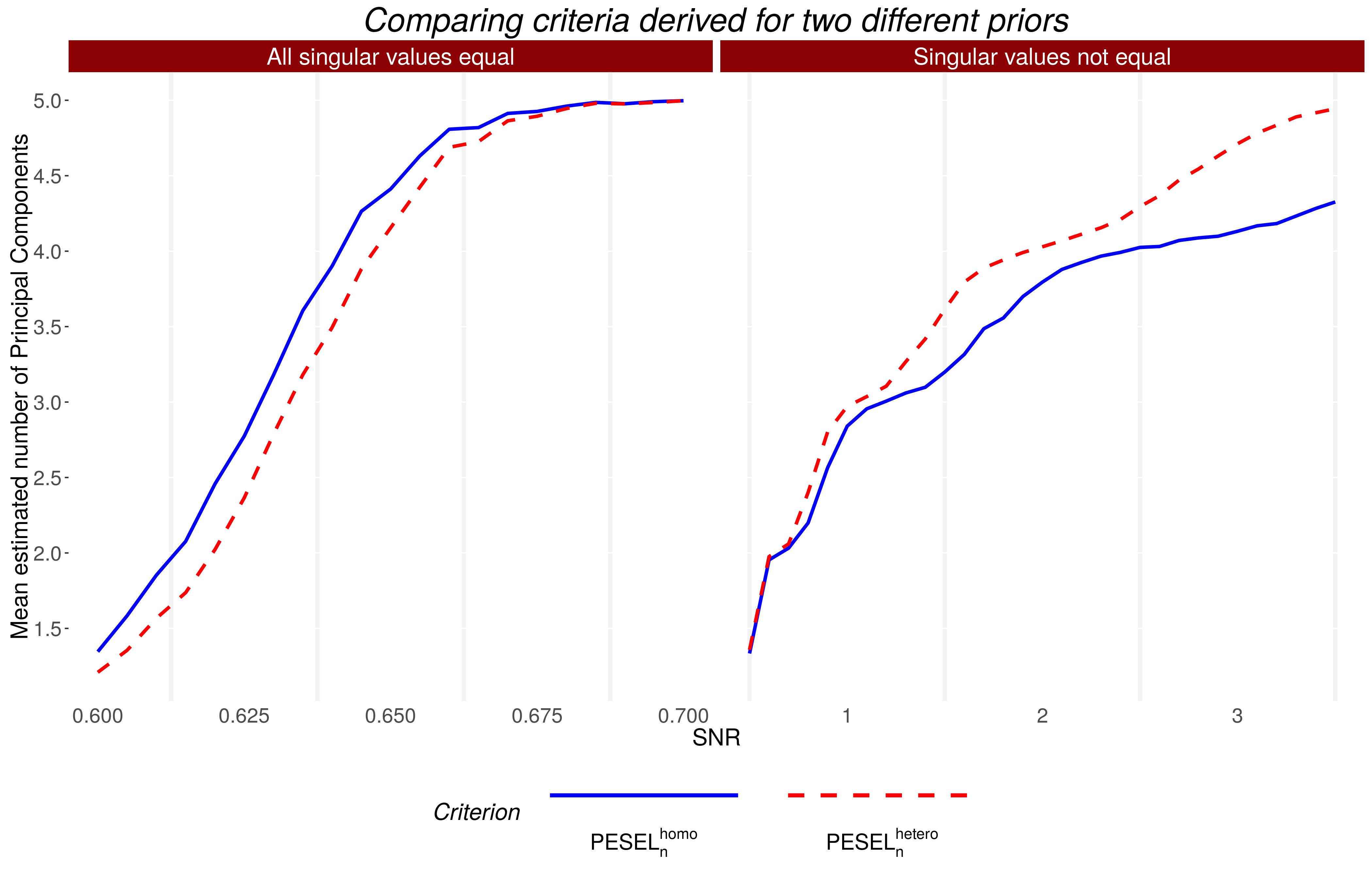
Figure 1: Comparison of performance for $PESEL^{hetero}_{n}$ (15) and $PESEL^{homo}_{n}$ (18). Number of variables is 50, number of observations is 100. True number of PCs is 5. When singular values are equal, then homogenous PESEL has an edge over heterogenous PESEL and vice versa.

3.3.2 Data drawn according to the Scenario 2

Figure 2 illustrates the performance of different methods when number of observations $n$ is either very large or very small compared to the number of variables $p$. Results are not surprising, as methods that assume asymptotics in $n$ work better when $n$ is large and vice versa. Note, that probabilistic methods outperform GCV when $\frac{p}{n}$ ratio is in accordance with their underlying asymptotics. In particular $PESEL_{p}$ is superior to all other approaches when $p>>n$. In case when $n>>p$ we observe a superior performance of the criterion of [Minka, 2000] based on extended version of Laplace approximation.

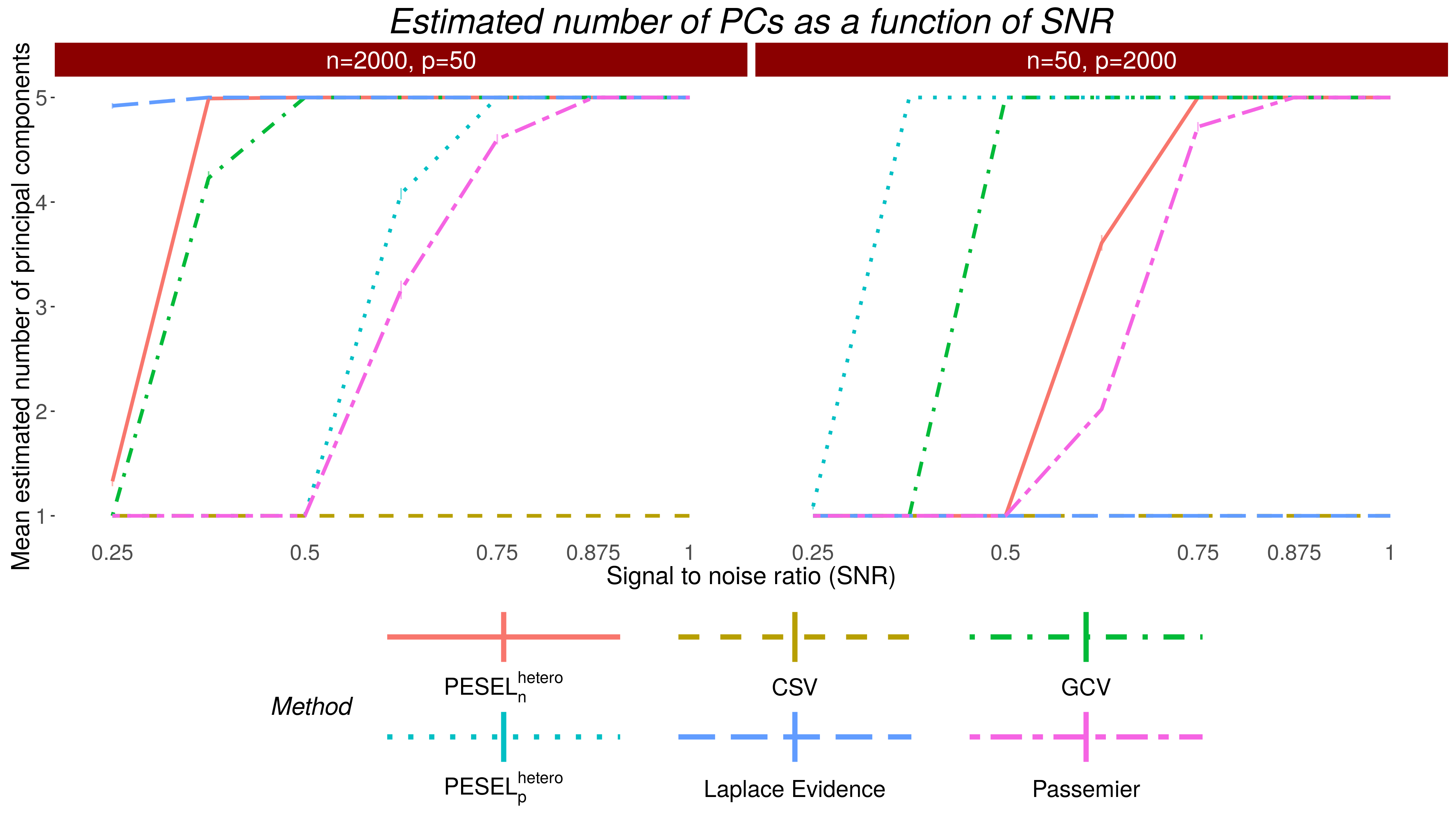
Figure 2: Data generated according to the Scenario 2. True number of components is 5. Results are for $n=2000$, $p=50$ and $n=50$, $p=2000$.

Figure 3 illustrates the situation when data is drawn according to the Scenario 2, but with number of variables and observations more balanced. As expected $PESEL^{hetero}_{n}$ is slightly worse than $PESEL^{hetero}_{p}$ when $p>n$. GCV works better when signals are weak and number of variables is comparable to number of observations. Passemier’s discriminant criterion is inferior to both PESELs. Laplace evidence performs poorly when the number of variables is big compared to the number of observations. CSV works well with weak signals and small number of variables, however, when either one of those grows, it encounters numerical problems described in Section 3.1.

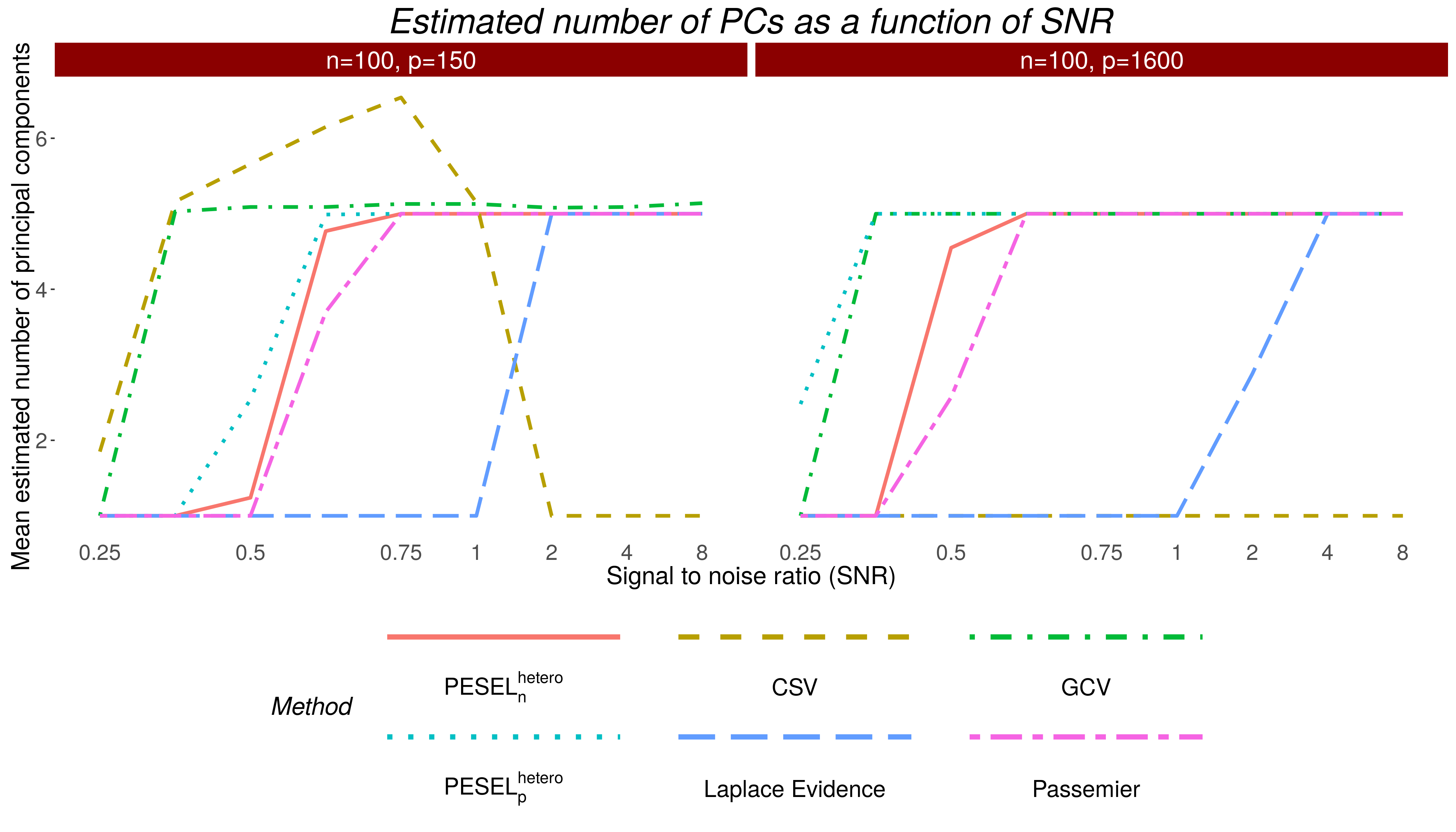
Figure 3: Data generated according to the Scenario 2. True number of components is 5. Results are for number of variables 150 and 1600. Number of observations is constant and equal 100.

3.3.3 Robustness

As mentioned in the Introduction, the main motivation for testing robustness is when PCA is used as an auxiliary technique. In such a case it might have to deal with data with an excessive noise. We report results for two kinds of violations of assumed probabilistic model, previously described in Section 3.2.

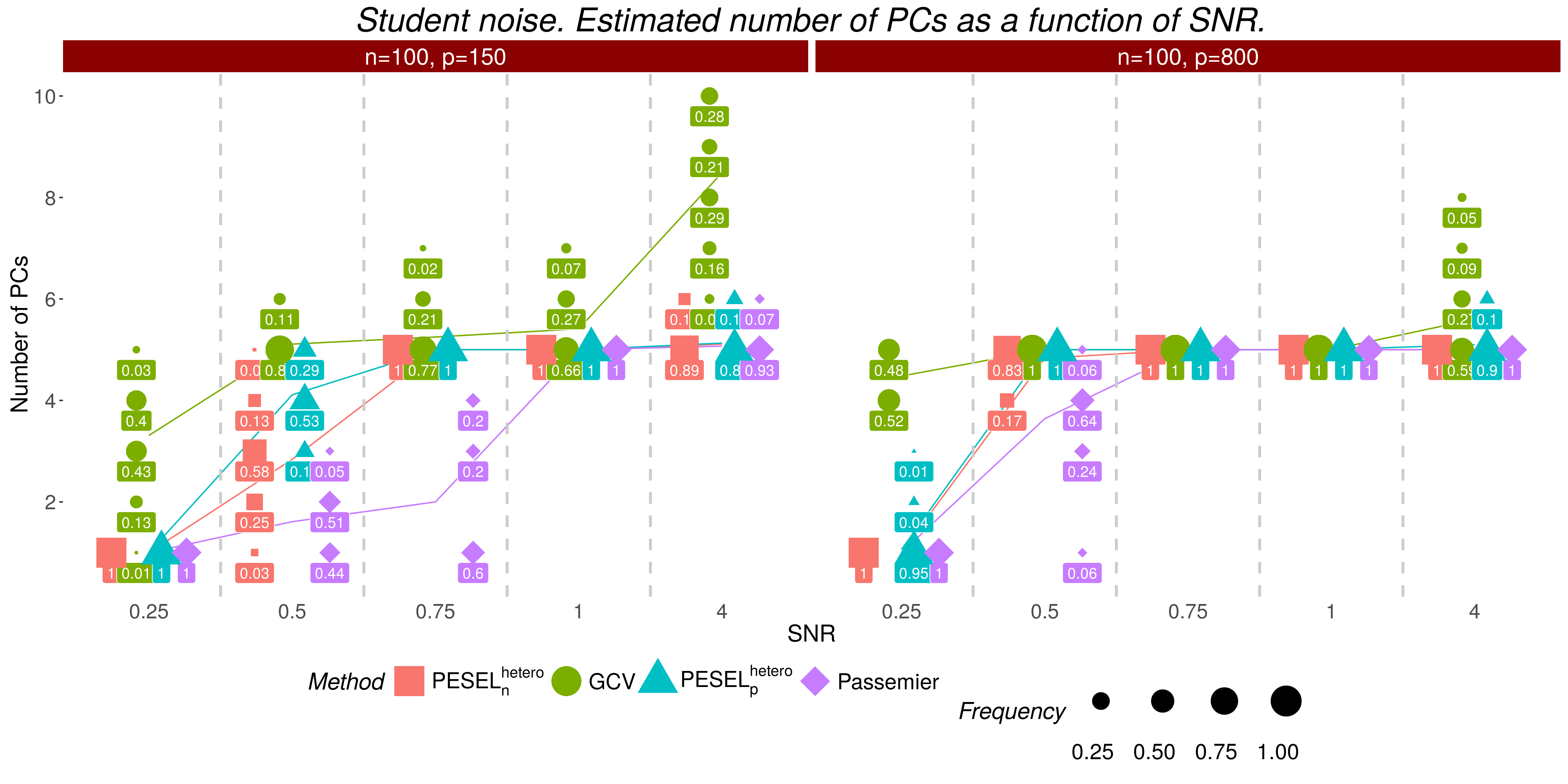
Figure 4: Data drawn according to the Scenario 3 (noise from Student distribution). True number of components is 5. Size of the symbol is proportional to the particular results frequency. Lines represent mean estimated number of Principal Components. Results are for number of variables 150 and 800. Number of observations is constant and equal 100.

For the clarity of plots, in Figures 4, 5 and 6 we selected only 4 methods for a detailed comparison. We observe that in case of violations of model assumptions GCV has a tendency to overestimate the number of components when signal gets stronger. Passemier is consistently inferior to $PESEL$. $PESEL_{p}^{hetero}$ is inferior to GCV when signal is weak, but does not overestimate the number of principal components when either number of variables or SNR grows.

As for the methods not included in the plots, $PESEL_{p}^{homo}$ behaves comparably to $PESEL_{p}^{hetero}$. Laplace evidence proves to be least robust, as it has a tendency to underestimate number of PCs when probabilistic model is violated. It is also highly dependent on assumed asymptotics i.e. $n>>p$. For CSV, when signal gets strong or number of variables gets large, it is becoming increasingly difficult to compute any of the integrals that this method is based on. As a result, we did not manage to use this method to estimate the number of PCs under such scenarios.

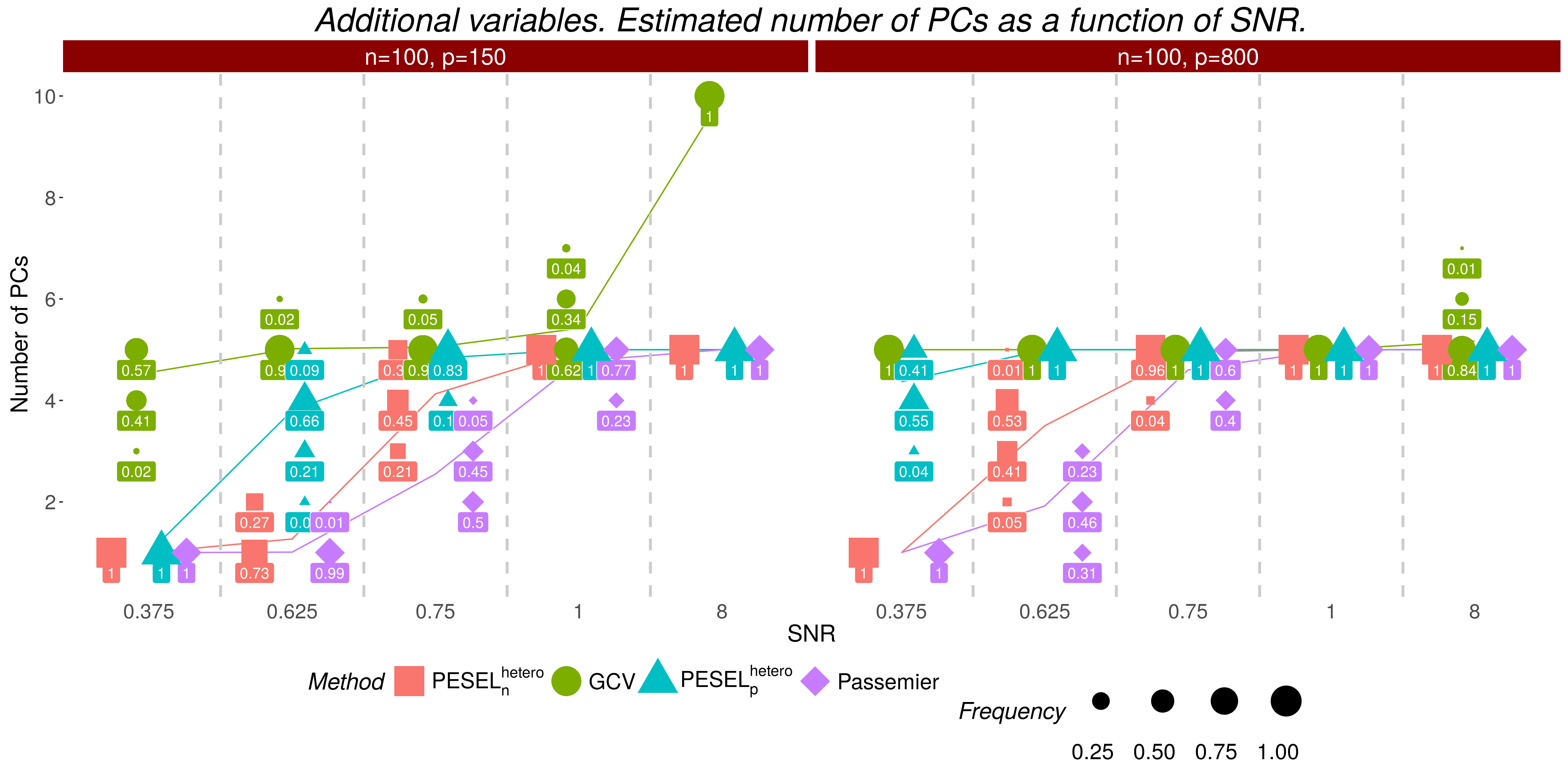
Figure 5: Data drawn according to the Scenario 4 (surplus noisy variables). True number of components is 5. Size of the symbol is proportional to the particular results frequency. Lines represent mean estimated number of Principal Components. Results are for number of variables 150 and 800. Number of observations is constant and equal 100.

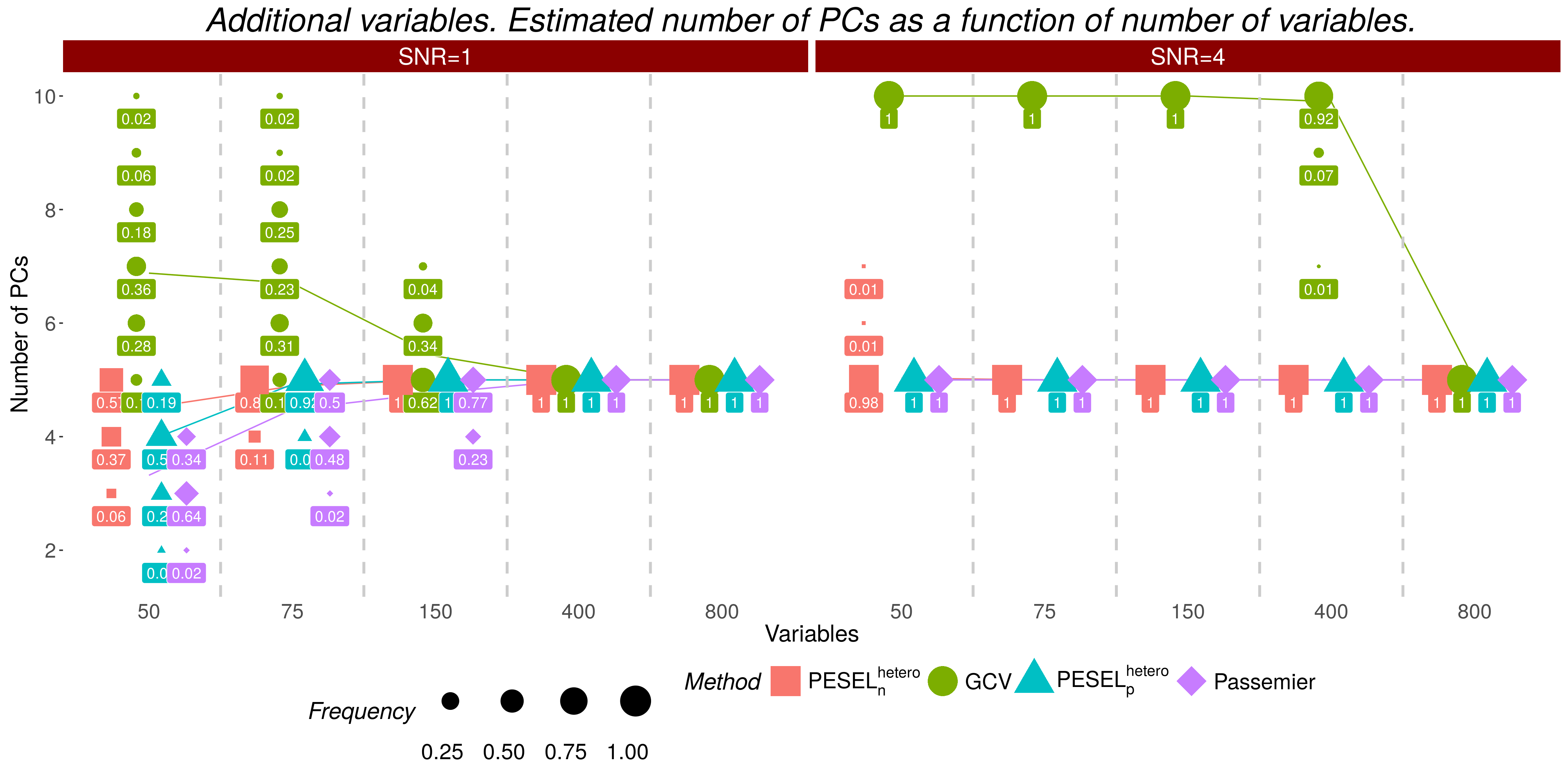
Figure 6: Data drawn according to the Scenario 4 (surplus noisy variables). True number of components is 5. Size of the symbol is proportional to the particular results frequency. Lines represent mean estimated number of Principal Components. Results are for signal to ratios 1 and 4. Number of variables varies from 50 to 800. Number of observations is constant and equal 100.

3.3.4 Simulations results summary

All in all, $PESEL_{p}$ performance is competitive to up-to-date methods. Note that GCV is a serious competitor for data drawn according to Scenario 2, however, when $p$ is large compared to $n$, which is our main focus, $PESEL_{p}$ is better. Similar conclusions come from robustness study, despite the fact that $PESEL_{p}$ was derived under specific probabilistic assumptions. When number of variables is large compared to number of observations, its performance is superior to competing methods. With small number of variables and strong signal it is less prone to overfitting than GCV.

3.4 Real data example

We use dataset UrineSpectra from [Nyamundanda et al., 2010] R package, which contains NMR metabolomic spectra from urine samples of mice. This datasets consist of 18 observations of 189 variables. Mice are from two groups, treatment and control group. We compared BIC for PPCA programmed in this package, equivalent to $PESEL^{hetero}_{n}$, with $PESEL^{hetero}_{p}$.

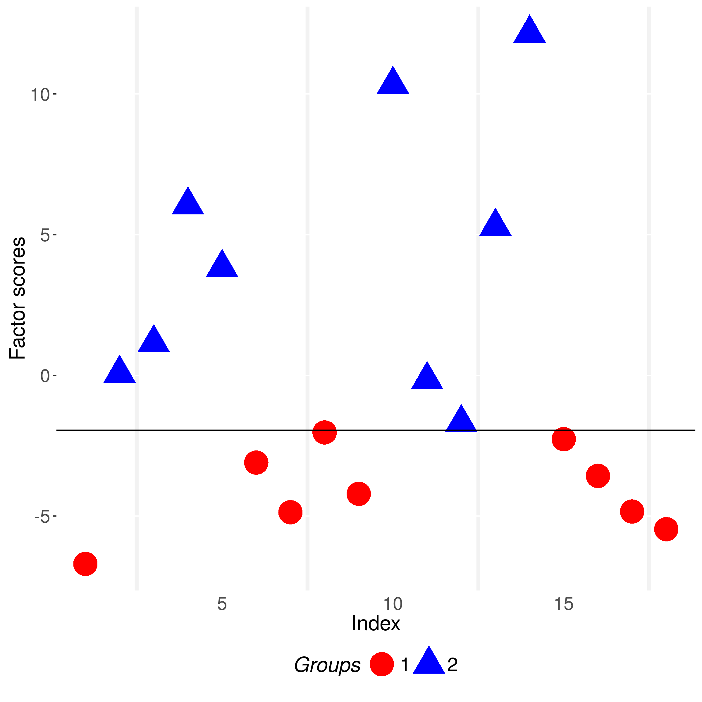
Figure 7: PC scores versus treatment group

Observe in Figure 7 that first principal component scores allow for perfect discrimination between two groups (treatment and control). In fact, our method chooses one principal component, while BIC for PPCA suggests that the true number of principal components is two. It means that our criterion is able to choose smaller and yet sufficient number of PCs. In other words, it provides parsimonious model by more restrictive, at least in this case, dimensionality reduction. In this data set the number of variables is substantially larger than the number of observations ($p>>n$), therefore this results is in accordance with intuitions and simulations presented previously.

4 Conclusion

We presented Bayesian approach for selecting the number of principal components in PCA. Starting from a fixed effect model (2), we presented a framework for approximating posterior probability. As number of parameters in model (2) is too big to apply Laplace approximation, we suggest imposing prior on either matrix $\mathbf{T}$ of PCA scores or matrix $\mathbf{W}$ of PCA loadings. Obtained PEnalized SEmi-integrated Likelihood ($PESEL$) is valid when either number of observations or number of variables tends to infinity, while the latter remains fixed. We compared performance of derived criteria with state-of-the-art methods in simulations. Although $PESEL$ assumes specific probabilistic model, simulation results suggest that it is more robust than existing methods, especially in a setting $p>>n$.

$PESEL$ can be used as an automatic tool for selecting the number of PCs. One of possible applications are clustering algorithms similar to [Agarwal and Mustafa, 2004]. $PESEL$ is implemented in the free software R [R Core Team, 2015] package varclust [Sobczyk et al., 2015], where it is used in an iterative variables clustering procedure.

$PESEL$ works in a specific asymptotics when one of $p$ and $n$ is fixed while latter tends to infinity. In case when both these parameters diverge it is not longer justified to use the Laplace approximation. In case when $p$ and $n$ diverge at the same rate Hoyle [2008] proposed an approximate Bayesian solution which uses more terms in the asymptotic expansion of the integrated likelihood. Contrary to PESEL this method is dependent on the selection of priors on both $T$ and $W$. We did not consider this approach in our simulation study because of the lack of the publicly available implementation. However, it is worth mentioning that the method of  [Passemier et al., 2015] is also designed to work under the assumption that $p$ and $n$ diverge to infinity at the same rate and that PESEL proved to be consistently superior than [Passemier et al., 2015] in a range of dimensions that was of our interest.

Finally, we would like to note that our approach can be easily extended for the cases when matrix $\mathbf{X}$ is binary or its elements can take on only integer values. Such data can be modeled using the framework of generalized linear models and the respective Bayesian approach for PCA was proposed e.g. in Hoff [2007]. Verification of the performance of PESEL under this setting remains an interesting topic for a further research.

Acknowledgment

We thank professor Jean-Michel Marin from University of Montpellier for assistance and for comments that improved the manuscript. PS and MB were supported by the European Union’s 7th Framework Programme for research, technological development and demonstration under Grant Agreement no 602552, cofinanced by the Polish Ministry of Science and Higher Education under Grant Agreement 2932/7.PR/2013/2. Calculations have been carried out in Wroclaw Centre for Networking and Supercomputing (http://www.wcss.pl), grant No. 347.

Appendix A Laplace approximation

Laplace approximation is a technique for rough calculation of special kind of integrals that are difficult or impossible to compute analytically. We shall present its multivariate form for the logarithm of the integral

$$\log\left(\int_{\mathbb{R}^{d}}g(\theta)e^{-th(\theta)}d\theta\right)\rightarrow th(\hat{\theta})+\frac{d}{2}\log{2\pi}+\frac{1}{2}\det\Sigma_{\hat{\theta}}-\frac{d}{2}\log{t},\;\;\mbox{as}\;\;t\rightarrow\infty\;\;,$$ (24)

where $\hat{\theta}=\operatorname*{arg\,max}_{\theta}\{-h(\theta)\}$ and $\Sigma_{\hat{\theta}}$ is a Hessian of $h(\raisebox{-1.07639pt}{\scalebox{1.5}{$\cdot$}})$ evaluated at $\hat{\theta}$. The above holds under some mild regularity conditions for $g(\cdot)$ and $h(\cdot)$ described in detail in e.g. [de Bruijn, 1970].

If we omit terms that do not depend on $t$ we get the approximation

$$\log\left(\int_{\mathbb{R}^{d}}g(\theta)e^{-th(\theta)}d\theta\right)\approx th(\hat{\theta})-\frac{d}{2}\log{t}.$$ (25)

In the context of statistical model selection let $\mathbf{Y}=\{Y_{1},...,Y_{N}\}$ be iid sample drawn from the distribution with the density or mass function $P(y|M,\theta)$, where $M$ denotes a given model and $\theta$ – parameters in that model. Moreover, let $\pi_{M}(\theta)$ be the prior distribution on those parameters. In case when all considered models have the same prior probability, the model selection according to the Maximum A Posteriori rule (MAP) is based on maximization of the marginal likelihood of the data $P(\mathbf{Y}|M)$, given by the formula

$$\log{P(\mathbf{Y}|M)} =\log\left(\int_{\Theta}P(\mathbf{Y}|M,\theta)\,\pi_{M}(\theta)\,d\theta\right)$$

$$=\log\left(\int_{\Theta}\pi_{M}(\theta)\exp\left\{-N\left(-\frac{1}{N}\log P(\mathbf{Y}|M,\theta)\right)\right\}d\theta\right)$$

$$=\log\left(\int_{\Theta}\pi_{M}(\theta)\exp\left\{-N\left(-\frac{\sum_{i}\log P(Y_{i}|M,\theta)}{N}\right)\right\}d\theta\right).$$

To use Laplace approximation observe that we can refer directly to formula (25), where $N$ corresponds to $t$, the prior $\pi_{M}(\cdot)$ to $g(\cdot)$ and averaged likelihood $\frac{\sum_{i}\log P(Y_{i}|\theta)}{N}$ to $h(\theta)$. By performing this approximation we get the classical BIC criterion

$$\log\left(\int_{\Theta}P(Y|M,\theta)\,\pi_{M}(\theta)\,d\theta\right)\approx\sum_{i}\log P(Y_{i}|M,\hat{\theta})-\frac{d}{2}\log{N}=\log P(\mathbf{Y}|M,\hat{\theta})-\frac{d}{2}\log{N}.$$

Appendix B Number of parameters in semi-integrated likelihood

Let us first decompose matrix $\mathbf{W}$, as in (12):

$$\mathbf{W} =\mathbf{U}(\mathbf{L}-\sigma^{2}\mathbf{I}_{k})^{1/2}\mathbf{R},$$

$$\mathbf{U}^{T}\mathbf{U} =\mathbf{I}_{k},$$

$$\mathbf{R}^{T}\mathbf{R} =\mathbf{I}_{k}.$$

This implies the following equality:

$$\mathbf{W}\mathbf{W}^{T}+\sigma^{2}\mathbf{I}_{p} =\mathbf{U}(\Lambda_{k}-\sigma^{2}\mathbf{I}_{k})^{1/2}\mathbf{R}(\mathbf{U}(\Lambda_{k}-\sigma^{2}\mathbf{I}_{k})^{1/2}\mathbf{R})^{T}+\sigma^{2}\mathbf{I}_{p}=$$

$$=\mathbf{U}(\Lambda_{k}-\sigma^{2}\mathbf{I}_{k})^{1/2}\mathbf{R}\mathbf{R}^{T}(\Lambda_{k}-\sigma^{2}(\mathbf{I}_{k})^{1/2}))^{T}\mathbf{U}^{T}+\sigma^{2}\mathbf{I}_{p}=$$ (26)

$$=\mathbf{U}(\Lambda_{k}-\sigma^{2}\mathbf{I}_{k})\mathbf{U}^{T}+\sigma^{2}\mathbf{I}_{p}.$$

In the above we use the fact, that $\mathbf{R}$ is orthogonal square matrix.

Using B we can write likelihood (2.2.1) for whole data as:

$$p(\mathbf{X}|\mu,\mathbf{W},\sigma^{2}) =\Pi^{n}_{i=1}p(\mathbf{x}_{i,\cdot}|\mu,\mathbf{W},\sigma^{2})$$

$$=(2\pi)^{-pn/2}|\mathbf{W}\mathbf{W}^{T}+\sigma^{2}\mathbf{I}_{p}|^{-n/2}\exp\left[-\frac{1}{2}tr((\mathbf{W}\mathbf{W}^{T}+\sigma^{2}\mathbf{I}_{p})^{-1}\mathbf{S})\right]$$

$$=(2\pi)^{-pn/2}|\mathbf{U}(\Lambda_{k}-\sigma^{2}\mathbf{I}_{k})\mathbf{U}^{T}+\sigma^{2}\mathbf{I}_{p}|^{-n/2}\exp\left[-\frac{1}{2}tr\left((\mathbf{U}(\Lambda_{k}-\sigma^{2}\mathbf{I}_{k})\mathbf{U}^{T}+\sigma^{2}\mathbf{I}_{n})^{-1}\mathbf{S}\right)\right].$$ (27)

We assume that priors on all parameters are independent. Then, since $\mathbf{R}$ is not part of likelihood B, it can be integrated out. So the integral in (2.2.1) reduces to

$$\int p(\mathbf{X}|\mu,\mathbf{W},\sigma^{2})d\mu\;d\mathbf{W}\;d\sigma^{2}=\int p(\mathbf{X}|\mu,\mathbf{U},\mathbf{L},\mathbf{R},\sigma^{2})d\mu\;d\mathbf{U}\;d\mathbf{L}\;d\mathbf{R}\;d\sigma^{2}=\int p(\mathbf{X}|\mu,\mathbf{U},\mathbf{L},\sigma^{2})d\mu\;d\mathbf{U}\;d\mathbf{L}\;d\sigma^{2}.$$ (28)

For $\mathbf{U}$ we have $pk-\frac{k(k+1)}{2}$ parameters – this is a dimension of $p\times k$ Steifel manifold [James, 1954]. $\mathbf{L}$ has $k$ parameters. $\mu$ has $p$ parameters and $\sigma$ is one parameter.

References

- Agarwal and Mustafa [2004] Agarwal, P. K. and Mustafa, N. H. K-means projective clustering. In Proceedings of the Twenty-third ACM SIGMOD-SIGACT-SIGART Symposium on Principles of Database Systems, PODS ’04, pages 155–165, New York, NY, USA, 2004. ACM. ISBN 158113858X.
- Allen et al. [2014] Allen, G. I.; Grosenick, L., and Taylor, J. A generalized least-square matrix decomposition. Journal of the American Statistical Association, 109(505):145–159, 2014.
- Bai and Ng [2002] Bai, J. and Ng, S. Determining the number of factors in approximate factor models. Econometrica, 70(1):191–221, 2002.
- Bishop [1999a] Bishop, C. M. Bayesian pca. In Proceedings of the 1998 Conference on Advances in Neural Information Processing Systems II, pages 382–388, Cambridge, MA, USA, 1999a. MIT Press. ISBN 0-262-11245-0.
- Bishop [1999b] Bishop, C. M. Variational principal components. In Proceedings Ninth International Conference on Artificial Neural Networks, ICANN’99, volume 1, page 509–514. IEE, January 1999b.
- Caussinus [1986] Caussinus, H. Models and uses of principal component analysis. In de Leeuw, J.; Heiser, W.; Meulman, J., and Critchley, F., editors, Multidimensional data analysis, pages 149–178. DSWO Press, 1986.
- Chikuse [2003] Chikuse, Y. Statistics on special manifolds. Lecture notes in statistics. Springer, 2003. ISBN 9783540001607.
- Choi et al. [2014] Choi, Y.; Taylor, J., and Tibshirani, R. Selecting the number of principal components: estimation of the true rank of a noisy matrix. ArXiv e-prints, October 2014.
- D’agostino and Russell [2005] D’agostino, Ralph B. and Russell, Heidy K. Scree test. In Encyclopedia of Biostatistics. John Wiley & Sons, Ltd, 2005. ISBN 9780470011812.
- de Bruijn [1970] de Bruijn, N.G. Asymptotic Methods in Analysis. Bibliotheca mathematica. Dover Publications, 1970. ISBN 9780486642215.
- Dempster et al. [1977] Dempster, A. P.; Laird, N. M., and Rubin, D. B. Maximum likelihood from incomplete data via the em algorithm. JOURNAL OF THE ROYAL STATISTICAL SOCIETY, SERIES B, 39(1):1–38, 1977.
- Hastie and Mazumder [2015] Hastie, T. and Mazumder, R. softImpute: Matrix Completion via Iterative Soft-Thresholded SVD, 2015. URL https://CRAN.R-project.org/package=softImpute. R package version 1.4.
- Hoff [2007] Hoff, P. D. Model averaging and dimension selection for the singular value decomposition. Journal of the American Statistical Association, 2007.
- Hoyle [2008] Hoyle, D. C. Automatic pca dimension selection for high dimensional data and small sample sizes. Journal of Machine Learning Research, 9(12):2733–2759, 2008.
- Husson et al. [2010] Husson, F.; Lê, S., and Pagès, J. Exploratory Multivariate Analysis by Example Using R. Chapman & Hall, 2010. ISBN 978-1-4398-3580-7.
- Husson et al. [2014] Husson, F.; Josse, J.; Le, S., and Mazet, J. FactoMineR: Multivariate Exploratory Data Analysis and Data Mining with R, 2014. R package version 1.27.
- Ilin et al. [2010] Ilin, A.; Raiko, T., and Jaakkola, T. Practical approaches to principal component analysis in the presence of missing values. JMLR, pages 1957–2000, 2010.
- Jackson [1993] Jackson, D. A. Stopping rules in principal components analysis: a comparison of heuristical and statistical approaches. Ecology, pages 2204–2214, 1993.
- James [1954] James, A. T. Normal multivariate analysis and the orthogonal group. Ann. Math. Statist., 25(1):40–75, 03 1954.
- Jolliffe [2002] Jolliffe, I.T. Principal Component Analysis. Springer Series in Statistics. Springer, 2002. ISBN 9780387954424.
- Josse and Husson [2012] Josse, J. and Husson, F. Selecting the number of components in principal component analysis using cross-validation approximations. Computational Statistics & Data Analysis, 56(6):1869 – 1879, 2012.
- Josse et al. [2009] Josse, J.; Husson, F., and Pagès, J. Gestion des données manquantes en analyse en composantes principales. Journal de la Société Française de Statistique, 150(2):28–51, 2009.
- Josse et al. [2011] Josse, J.; Pagès, J., and Husson, F. Multiple imputation in principal component analysis. Advances in Data Analysis and Classification, 5(3):231–246, 2011. ISSN 1862-5355.
- Minka [2000] Minka, T. P. Automatic choice of dimensionality for pca. NIPS, 13:514, 2000.
- Nyamundanda et al. [2010] Nyamundanda, G.; Gormley, I. C., and Brennan, L. MetabolAnalyze: probabilistic principal components analysis for metabolomic data, 2010. R package version 1.3.
- Owen and Perry [2009] Owen, A. B. and Perry, P. O. Bi-cross-validation of the svd and the nonnegative matrix factorization. Ann. Appl. Stat., 3(2):564–594, 06 2009.
- Passemier et al. [2015] Passemier, D.; Li, Z., and Yao, J. On estimation of the noise variance in high-dimensional probabilistic principal component analysis. Journal of the Royal Statistical Society Series B, 2015.
- Pearson [1901] Pearson, K. On lines and planes of closest fit to systems of points in space. Philosophical Magazine, 2(11):559–572, 1901.
- R Core Team [2015] R Core Team, . R: A Language and Environment for Statistical Computing. R Foundation for Statistical Computing, Vienna, Austria, 2015.
- Rajan and Rayner [1997] Rajan, J.J. and Rayner, P.J.W. Model order selection for the singular value decomposition and the discrete karhunen-loeve transform using a bayesian approach. Vision, Image and Signal Processing, IEE Proceedings -, 144(2):116–123, Apr 1997. ISSN 1350-245X.
- Sobczyk et al. [2015] Sobczyk, P.; Josse, J., and Bogdan, M. varclust: Clustering of variables, 2015. R package version 0.95.
- Tipping and Bishop [1999] Tipping, M. E. and Bishop, C. M. Probabilistic principal component analysis. Journal of the Royal Statistical Society, Series B, 61:611–622, 1999.