The Field White Dwarf Mass Distribution

Abstract

We revisit the properties and astrophysical implications of the field white dwarf mass distribution in preparation of Gaia applications. Our study is based on the two samples with the best established completeness and most precise atmospheric parameters, the volume-complete survey within 20 pc and the Sloan Digital Sky Survey (SDSS) magnitude-limited sample. We explore the modelling of the observed mass distributions with Monte Carlo simulations, but find that it is difficult to constrain independently the initial mass function (IMF), the initial-to-final-mass relation (IFMR), the stellar formation history (SFH), the variation of the Galactic disk vertical scale height as a function of stellar age, and binary evolution. Each of these input ingredients has a moderate effect on the predicted mass distributions, and we must also take into account biases owing to unidentified faint objects (20 pc sample), as well as unknown masses for magnetic white dwarfs and spectroscopic calibration issues (SDSS sample). Nevertheless, we find that fixed standard assumptions for the above parameters result in predicted mean masses that are in good qualitative agreement with the observed values. It suggests that derived masses for both studied samples are consistent with our current knowledge of stellar and Galactic evolution. Our simulations overpredict by 40-50% the number of massive white dwarfs ($M>0.75$ $M_{\odot})$ for both surveys, although we can not exclude a Salpeter IMF when we account for all biases. Furthermore, we find no evidence of a population of double white dwarf mergers in the observed mass distributions.

1 Introduction

Stars are an integral part of the luminous baryonic component of galaxies. As a consequence, the IMF and SFH are important parameters in galactic evolution models. Both quantities can be studied from a comparison of spectral population synthesis models with samples of galaxies at different redshifts (see, e.g., Maraston, 2005; Daddi et al., 2007; Conroy et al., 2010). Furthermore, resolved stellar populations in the the Milky Way and nearby galaxies inform us more directly on the IMF (see, e.g., Kroupa et al., 1993; Chabrier, 2003; Bastian et al., 2010). In particular, recent Hubble Space Telescope observations of young clusters in M31 (see, e.g., Weisz et al., 2015) suggest that the high-mass IMF above $M\gtrsim 2M_{\odot}$ is on average slightly steeper than the commonly used Salpeter (1955) model.

Young and massive star clusters are ideal for studying the high-mass IMF since they still include bright intermediate-mass stars ($1.5\lesssim M/M_{\odot}\lesssim 8$). However, the vast majority of these stars that were ever born in the local galaxy group are now white dwarfs. While these faint remnants can not be observed to the same distances as their progenitors, the field white dwarf mass distribution could still provide information about the IMF of local populations, such as the Galactic disk and halo. Current white dwarf samples are small for Galactic halo studies but Gaia (Carrasco et al., 2014) and Euclid (Laureijs et al., 2011) will soon present unprecedented opportunities. Furthermore, the mass distribution of degenerate stars presents unique constraints on the population of white dwarf mergers, which could be one of the evolution channel linked to SN Ia (see, e.g., Dan et al., 2015) as well as high-field magnetic white dwarfs (B $>$ 1 MG; Tout et al., 2004, 2008; García-Berro et al., 2012; Wickramasinghe et al., 2014). Extensive studies have also been dedicated to using white dwarf masses and cooling ages to derive the SFH (Tremblay et al., 2014) and IFMR (see, e.g., Weidemann, 2000; Catalán et al., 2008; Kalirai et al., 2008; Williams et al., 2009; Dobbie et al., 2012; Cummings et al., 2015, 2016a). The IFMR provides constraints on the luminosity and lifetime of bright AGB stars, hence on stellar population synthesis models (Marigo & Girardi, 2007; Kalirai et al., 2014). While these SFH and IFMR studies rely on individual stellar parameters, an understanding of the overall field white dwarf mass distribution leads to an essential internal consistency check for white dwarf and Galactic evolution models.

Most of the $\sim$30,000 degenerate stars spectroscopically identified in the SDSS (Alam et al., 2015) have published masses (Tremblay et al., 2011; Kleinman et al., 2013; Kepler et al., 2016), and among them $\sim$3000 have sufficiently high signal-to-noise (S/N $\gtrsim 15$) to clearly define the white dwarf mass distribution. In particular, the sample is large enough to have outstanding statistics on less common high-mass white dwarfs (M $>$ 0.75 $M_{\odot}$). However, difficulties in the interpretation of the SDSS mass distribution arise from significant spectroscopic selection biases as a function of colour and magnitude (De Gennaro et al., 2008; Gentile Fusillo et al., 2015). The local 20 pc sample (Holberg et al., 2008; Sion et al., 2009; Giammichele et al., 2012; Sion et al., 2014) offers a better completeness but is limited to $\sim$120 objects. In all cases, multiple astrophysical effects have to be considered when attempting to comprehend field white dwarf masses, such as the SFH, IMF, IFMR, and binary evolution. Nevertheless, a few attempts have been made at understanding features in the observed white dwarf mass distributions (Ferrario et al., 2005; Catalán et al., 2008; Rebassa-Mansergas et al., 2011). In the recent years, most of these studies have been aimed at identifying a population of mergers, though there are currently different interpretations on whether there is evidence for merger products (Liebert et al., 2005; Ferrario et al., 2005; Giammichele et al., 2012; Wegg & Phinney, 2012; Isern et al., 2013; Rebassa-Mansergas et al., 2015). To our knowledge, there was no extensive study connecting white dwarf mass distributions to Galactic archeology. This is in contrast to white dwarf luminosity functions that have been employed to derive the age and formation history of the Galactic disk (see, e.g., Winget et al., 1987; Harris et al., 2006; Rowell, 2013).

The initial goal of this study was to constrain the IMF from white dwarf mass distributions drawn from the 20 pc and SDSS samples. We rapidly found out that uncertainties in astrophysical relations and biases prevent a straightforward interpretation, much in contrast with our earlier study of the SFH from the local 20 pc white dwarf sample (Tremblay et al., 2014). In this work, we present instead a systematic review of the uncertainties that come into play when interpreting white dwarf mass distributions. Our investigation will help to comprehend the larger Gaia sample that will soon provide precise individual luminosities for almost all known white dwarfs (Carrasco et al., 2014). By combining parallaxes with spectroscopic or photometric temperatures and a mass-radius relation, we will obtain precise masses independently from current spectroscopic surface gravity measurements. We will get much more precise mass distributions and gain a better understanding of the completeness of current samples.

We base our study on Monte-Carlo simulations considering the IMF, IFMR, SFH, main-sequence evolution, white dwarf evolution, galaxy kinematics, and survey biases. We explore the modelling of both the observed 20 pc and SDSS mass distributions. Since the white dwarfs studied in this work are restricted to distances below $\sim$500 pc, we made no attempt at a full scale model of the Galaxy. The assumptions behind our simulations are fairly similar to those employed in recent studies of white dwarf luminosity functions and kinematics (Wegg & Phinney, 2012; Verbeek et al., 2013; Torres et al., 2014; Cojocaru et al., 2015; Lam et al., 2015; Rebassa-Mansergas et al., 2015). As a consequence, we concentrate on the often overlooked white dwarf mass distributions. In Section 2 we describe our selected white dwarf samples. We continue with a description of our standard simulations in Section 3 followed by a lengthy discussion of uncertainties (Section 4). We comment on the results in Section 5 and conclude in Section 6.

2 White Dwarf Samples

The absolute magnitude of a white dwarf is strongly dependent on its mass and age. In order to study mass distributions, it is therefore essential to have a clear assessment of the completeness of the observed samples. As a consequence, we restrict our study to two white dwarf samples whose completeness has been extensively characterised. Those correspond to the volume-complete 20 pc survey, as well as the largely magnitude-limited SDSS sample. Below $M_{\rm WD}\sim 0.45~{}M_{\sun}$, all objects are thought to be He-core white dwarfs that are the product of close binary evolution. Assuming single star evolution, these objects would have main-sequence lifetimes that are longer than the age of the Universe. We found it practical to simply remove those objects from the comparison of the observed and predicted mass distributions. Extensive population studies including binary evolution have already been performed (see, e.g., Toonen & Nelemans, 2013; Camacho et al., 2014) and it is outside the scope of our investigation to review these results. Throughout this work, all our quoted values are for white dwarf masses above 0.45 $M_{\sun}$. The main properties of our observed samples are identified in Table LABEL:fg:t0 and described below.

2.1 20 pc Sample

We rely on the local 20 pc sample as presented in Table 3 of Giammichele et al. (2012) with their corrections for 3D convective effects (see their fig. 16). We have removed objects with estimated distances above 20 pc as well as 12 members with no mass determination for a total of 105 white dwarfs, among them 97 with $M>0.45M_{\odot}$. The atmospheric parameters were determined from a combination of photometric, spectroscopic, and parallax observations. In general, the combination of the photometric fluxes with parallax allowed for the most precise luminosity and effective temperature ($T_{\rm eff}$) determinations. The masses were then derived employing the evolutionary models of Fontaine et al. (2001). These models have C/O cores (50/50 by mass fraction mixed uniformly) and assume thick hydrogen layers ($M_{\rm H}/M_{\rm total}$ = 10^-4) for H-atmosphere white dwarfs and thin layers ($M_{\rm H}/M_{\rm total}$ = 10^-10) for helium and mixed atmospheres.

Table 1: Observed Samples

Property	20 pc sample	SDSS sample
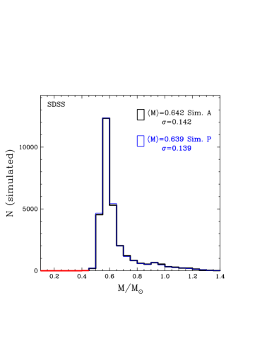
Sample definition	Giammichele et al. 2012	Kleinman et al. 2013
Data reduction	Various	SDSS DR10
$T_{\rm eff}$/$\log g$	Giammichele et al. 2012	This work
Cooling models	Fontaine et al. 2001	Fontaine et al. 2001
$T_{\rm eff}$ range (K)	Unrestricted	$16,000<T_{\rm eff}<22,000$
Magnitude range	Unrestricted	$16.0<g<18.5$
Mass range ($M_{\odot}$)	$>$ 0.45	$>$ 0.45
Distance range (pc)	$<$ 20	Unrestricted
Spectral types	Unrestricted	DA(Z) and DB(A)(Z)
Number	97	715
Number (non-DA)	34	135
Number (magnetic)	15	0

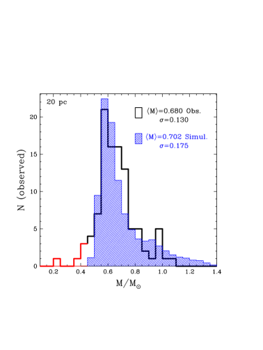
We present the observed mass distribution in Fig. 1. We remind the reader that by restricting the selected stars to $M>0.45~{}M_{\odot}$ the mean mass value is biased towards a higher value than those reported in other studies. This sample is estimated to be 80-90% volume-complete (Holberg et al., 2008; Giammichele et al., 2012; Tremblay et al., 2014). At zeroth order, the mass of a white dwarf is expected to have little dependence on the volume in which it is located. However, we discuss in Section 4 that biases owing to variable SFH and velocity dispersion (as a function of age and mass) have a significant impact on the interpretation of the observed mass distribution. We also pay special attention to the fact that the 10-20% missing objects could preferentially be lower luminosity, hence massive white dwarfs. We note that owing to the photometric technique which has little sensitivity to the atmospheric composition, this sample has precise masses for all spectral types, including DA, DB, DC, DQ, and DZ white dwarfs. This also includes magnetic objects accounting for 15% of the sample, which should be regarded as a lower limit given that many local white dwarfs have not been adequately observed for polarisation and many of them are too cool to show Zeeman splitting.

Figure 1: Observed (black) and simulated (filled blue) mass distributions for the 20 pc sample of Giammichele et al. (2012). The standard Monte Carlo simulation $A_{\rm 20pc}$ is described in Section 3. We neglect low-mass objects (red; $M<0.45~{}M_{\odot}$) for the computation of the mean masses and mass dispersions, which are labeled on the panel. This should taken into account when comparing to other studies that do not restrict mass values.

2.2 SDSS Sample

We also rely on the SDSS white dwarf sample, which is largely magnitude-limited but has a complex spectroscopic completeness that varies from 10 to 90% as a function of magnitude and colour (De Gennaro et al., 2008; Gentile Fusillo et al., 2015). The other major difference with the 20 pc sample is that no parallaxes are available for the vast majority of SDSS white dwarfs. For DA and DB white dwarfs, which represent roughly 85% of the SDSS sample (Kleinman et al., 2013), it is possible to employ the spectroscopic method combined with evolutionary sequences to determine the masses to a high precision (Bergeron et al., 1992, 2011). On the other hand, it is not straightforward to determine masses for other spectral types, in particular magnetic DA white dwarfs. The resulting bias on the mass distribution could be important, since magnetic degenerates are thought to be more massive than the average (Ferrario et al., 2015).

We base our analysis on the SDSS Data Release 7 (DR7) spectroscopic sample of Kleinman et al. (2013), where we have carefully refitted all DAs with 1D ML2/$\alpha$ = 0.8 model atmospheres (Tremblay et al., 2011), applied 3D corrections (Tremblay et al., 2013), and re-assigned the different subtypes based on a careful visual identification. We have employed SDSS spectra with the data reduction from DR10. As for the 20 pc sample, we have employed evolutionary models from Fontaine et al. (2001) to constrain masses. Tremblay et al. (2011) have demonstrated that a cutoff at S/N $\sim$ 15 was an optimal separation between the size of the sample and the uncertainties in the mass distribution, and we use a corresponding cutoff at $g<18.5$.

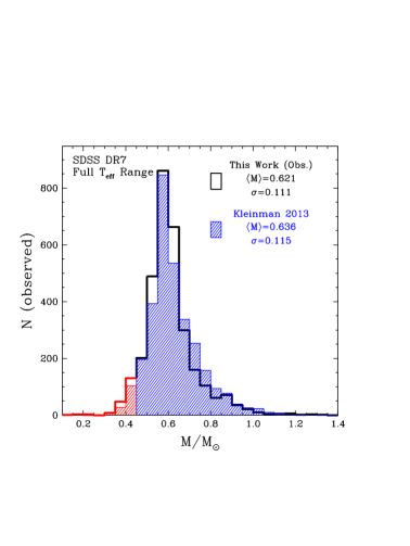
The full results of our alternative analysis are outside the scope of this work, and in Fig. 2 we simply compare our mass distribution with that of Kleinman et al. (2013). We restrict the comparison to single non-magnetic DAs ($M<0.45~{}M_{\odot}$) and we note that the identification of subtypes differs between the two studies. We find a moderate offset of 0.015 $M_{\odot}$ in the mean mass. Furthermore, our identification of subtypes is significantly different, especially for magnetic white dwarfs and DA+DC double degenerates, which can result in spurious high $\log g$ values if incorrectly identified. For instance, we find a magnetic fraction of 2.5% compared to 4.4%-5.3% for Kleinman et al. (2013), with their upper estimate based on uncertain detections. Our recovered fraction is admittedly small, 6 times less than for the 20 pc sample discussed above, and we have no explanation for this behaviour. The true magnetic incidence in the SDSS is expected to be slightly larger given the low average signal-to-noise of the spectroscopic observations, but this can not account for the full difference. We are aware that larger and more recent SDSS samples have since been identified, though until the discrepancy with the identification of subtypes has been resolved, we prefer to rely on our own sample. Furthermore, our study below is limited by biases rather than number statistics, hence it was deemed unnecessary to build a larger sample.

Figure 2: Comparison of the SDSS DR7 mass distributions from this work (black) and Kleinman et al. (2013, filled blue) for single, non-magnetic DA white dwarfs with $g<18.5$. The identification of subtypes differs between the two studies, hence we renormalise the Kleinman et al. (2013) distribution of 2903 single non-magnetic DAs to the 2998 such objects identified in this work. We neglect low-mass objects (red; $M<0.45~{}M_{\odot}$) for the computation of the mean masses and mass dispersions. Our reported mean masses are thus biased towards higher values than those previously published.

We complement our DA sample with the DB white dwarfs identified by Kleinman et al. (2013), using the atmospheric parameters recently determined by Koester & Kepler (2015). For this study, we rely only on the single DA and DB white dwarfs (including objects with trace elements such as DAZ or DBA), hence we remove stellar remnants with main-sequence companions, double degenerates, and magnetic white dwarfs. We nevertheless consider the effect of these missing subtypes in our review of uncertainties in Section 4.

Below $T_{\rm eff}\lesssim 12,000$ K, helium-rich DC, DQ, and DZ white dwarfs become present in significant numbers, and for $T_{\rm eff}<16,000$ K, DBs have uncertain spectroscopic parameters (Bergeron et al., 2011; Koester & Kepler, 2015). As a consequence, we restrict our study to higher temperatures where the large majority of SDSS white dwarfs have precise atmospheric parameters and are either of the DA, DB, or DBA spectral type. Furthermore, the spectroscopic completeness of the SDSS catalog varies significantly as a function of colour and magnitude. To circumvent this problem, we have decided to restrict our analysis of the mass distribution to objects with $16,000<T_{\rm eff}$ (K) $<22,000$ and $16.0<g<18.5$. This corresponds to cooling ages in the range $0.02\lesssim\tau$ (Gyr) $\lesssim 1$. We demonstrate in Fig. 3 that the completeness can be approximated as constant within that range. We base our calculations on the results of Gentile Fusillo et al. (2015) who have determined the probability of SDSS DR10 photometric sources of being white dwarfs based on colours and proper-motion. We have converted the observed colours into atmospheric parameters for DA white dwarfs, and we define the completeness as the fraction of objects with a spectrum among those that have a probability of 41% or larger of being a white dwarf. We note that the spectroscopic completeness appears to decrease slightly for higher masses, though one should be cautious about this result since we do not account for possible photometric calibration offsets, reddening, and a confirmation that objects without a spectrum are actually stellar remnants. We remind the reader that Fig. 3 refers to the spectroscopic completeness for a magnitude-limited sample, and not the volume completeness, which will be taken into account in our simulations in Section 3. DB white dwarfs span a similarly located but much smaller colour space in that $T_{\rm eff}$ range, hence we assume that the completeness is the same as for DAs. We concur with De Gennaro et al. (2008) that spectroscopic completeness corrections do not necessarily have a large effect on the relative mass distribution.

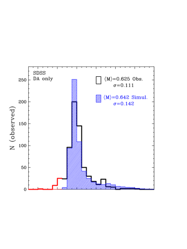
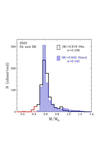
Fig. 4 presents the mass distribution for our selected $T_{\rm eff}$ and $g$ magnitude range, both for DAs only and the combined DA and DB sample. In the combined sample, the fraction of DBs is 18%. We find that the DA mass distribution (top panel) for our $T_{\rm eff}$ subsample is fairly similar to the mass distribution for the full temperature range in Fig. 2. We study further our $T_{\rm eff}$ cutoffs in Section 4 and Table 3. We also observe that the addition of DB white dwarfs (bottom panel) leads to a slightly smaller mean mass and mass dispersion. One reason is that there are very few genuine high-mass helium-rich degenerate stars when uncertainties in the line broadening are accounted (Bergeron et al., 2011). For the remainder of this work, we employ the combined DA and DB sample.

Figure 3: Spectroscopic completeness of the SDSS DR10 sample as a function of $T_{\rm eff}$ (top panel), $M/M_{\odot}$ (middle), and $g$ magnitude (bottom) for DA white dwarfs. We only cover the $T_{\rm eff}$ range studied in this work. For objects that have a probability of 41% or higher of being a white dwarf in Gentile Fusillo et al. (2015), we define the completeness as the fraction of objects with a SDSS spectrum. We have transformed the observed colours into atmospheric parameters with model atmospheres from Tremblay et al. (2011).

Figure 4: Top: observed (black) and simulated (filled blue) mass distributions for the SDSS DR7 DA white dwarf sample for $16,000<T_{\rm eff}$ (K) $<22,000$ and $16.0<g<18.5$. The standard Monte Carlo simulation $A_{\rm SDSS}$ is described in Section 3. We have removed binaries and magnetic white dwarfs from the observed sample. We neglect low-mass objects (red; $M<0.45~{}M_{\odot}$) for the computation of the mean masses and mass dispersions, which are labeled on the panel. Bottom: same as the top panel but for the combined DA and DB sample.

3 Simulations

We have designed Monte Carlo simulations of white dwarf populations in the solar neighborhood. The basic assumptions about these simulations are similar to the ones presented in Wegg & Phinney (2012); Cojocaru et al. (2015); Rebassa-Mansergas et al. (2015) and Torres & García-Berro (2016). In this section, we present our standard model for the 20 pc ($A_{\rm 20pc}$) and SDSS ($A_{\rm SDSS}$) samples, and defer the lengthy discussion about biases and alternative assumptions to Section 4.

We use a simple galactic model with a thin disk that was formed 10 Gyr ago, a constant star formation history (SFH), and a Salpeter initial mass function ($NdM_{\rm i}\propto M_{\rm i}^{-\alpha}dM_{\rm i}$, where $\alpha=2.35$). We assume a uniform distribution in Galactic coordinates $U$ and $V$, corresponding to the plane of the disk. This crude galactic model is a reasonable assumption given that all of our targets are within a distance of 500 pc. We suppose that radial migration within the disk has no net effect on the white dwarf mass distribution, which is also a consequence of assuming a uniform distribution in the plane of the disk.

We employ a variable scale height in the vertical direction $W$ as a function of total stellar age, the sum of the white dwarf cooling age and the main-sequence lifetime. We suppose that the vertical scale height is directly proportional to the observed vertical velocity dispersion $\sigma_{\rm W}$, as in the isothermal sheet galactic disk model (Spitzer, 1942). We use the empirical velocity dispersion versus total age relation from Seabroke & Gilmore (2007)

$$\sigma_{\rm W}=k~{}{\rm age}^{0.6}~{}~{}~{}~{}~{}{\rm for~{}total~{}stellar~{}age}<5{\rm~{}Gyr},$$ (1)

$$\sigma_{\rm W}=k~{}{\rm 5}^{0.6}~{}~{}~{}~{}~{}{\rm for~{}total~{}stellar~{}age}>5{\rm~{}Gyr},$$ (2)

where $k$ is a constant and the total stellar age in Gyr. We have chosen the constant so that the vertical scale height is 75 pc at 1 Gyr based on the velocity of young massive SDSS white dwarfs (Wegg & Phinney, 2012) and the scale height distribution of young open clusters (Buckner & Froebrich, 2014). The vertical scale height thus reaches a maximum value of $\sim$200 pc at 5 Gyr and thereafter remains constant according to Eqs. 1-2. Since white dwarfs have a quite limited mass range, we do not consider a variation with mass. Furthermore, our samples are centered 20 pc above the plane of the disk, which is the approximate position of the Sun.

The first step of our Monte Carlo simulations is to have a star formed at a random time in the last 10 Gyr, a random mass weighted by the Salpeter IMF, and a random location within 500 pc weighted by the exponential distribution in the vertical direction. We then derive the main-sequence lifetime for solar metallicity from Hurley et al. (2000), and subtract it to the formation time to obtain the white dwarf cooling age. If the cooling age is positive, we then obtain the white dwarf cooling age. If the cooling age is positive, we then find the white dwarf mass using an IFMR drawn from Cummings et al. (2016a) supplemented by low-mass data ($M_{\rm WD}<0.65M_{\odot}$) adapted from Kalirai et al. (2007, 2008, 2009).

$$M_{\rm WD}=0.541932-0.0184299M_{\rm i}+0.0265180M_{\rm i}^{2}\\ {\rm for~{}}M_{\rm i}<4M_{\odot}~{},$$ (3)

$$M_{\rm WD}=0.915738-0.0878731M_{\rm i}+0.0208688M_{\rm i}^{2}\\ {\rm for~{}}M_{\rm i}>4M_{\odot}~{},$$ (4)

where $M_{\rm WD}$ is the white dwarf mass and $M_{\rm i}$ is the initial mass. We are aware that the observed IFMR is often represented as a linear relation and that our two-part 2nd order fit may provide corrections to the linear relation that are not physical. However, the IFMR is an empirical relation and our 2nd order fit allows us to directly connect features in the observed IFMR to features in the mass distribution (Ferrario et al., 2005). Unlike the IMF, there is no theoretical suggestion that the IFMR should be a simple analytical function. In fact, several theoretical IFMRs have a turnover at $M_{\rm i}\sim 4M_{\odot}$ resulting from the second dredge-up which only occurs for higher masses (see, e.g., Marigo & Girardi, 2007; Meng et al., 2008).

From the white dwarf mass and cooling age, we obtain $T_{\rm eff}$ and $\log g$ with the evolution models of Fontaine et al. (2001), as well as $V$ and $g$ magnitudes from the model atmospheres of Tremblay et al. (2011) and Bergeron et al. (2011) for DA and DB white dwarfs, respectively. We use the observed number of H- and He-atmospheres. In all cases, we assume 70% of thick H-layers and 30% of thin H-layers, which is based on the fact that a fraction of DAs also have thin layers (Tremblay & Bergeron, 2008).

All further steps depend on the specific survey. In all cases, we let the simulations run long enough so that 30,000 white dwarfs satisfying all cuts are selected. We are only interested in relative numbers and we renormalise our mass distributions to the actual number of observed white dwarfs with M > 0.45 $M_{\odot}$, unless simulations are compared.

3.1 Simulations of the 20 pc Sample

We have simulated observational errors with a Gaussian error distribution and a 1$\sigma$ value based on the mean of the uncertainties given in Giammichele et al. (2012). It corresponds to 0.0375 $M_{\odot}$ in mass, 2.0% in temperature, and 0.7 pc in distance. The final selection is then made from all objects within 20 pc. Fig. 1 compares our simulated mass distribution with the observed one. We remind the reader that it is not a fit and we made no attempt to tweak the input parameters of the simulation to match the observations. We find that the agreement is quite good, both in terms of the mean mass and the overall shape of the distribution. However, the mass dispersion value and the number of massive white dwarfs are overpredicted in the simulations.

3.2 Simulations of the SDSS Sample

Fig. 5 illustrates that the mass error for DA white dwarfs in the SDSS is strongly correlated with magnitude. We made a linear fit to the $\log\sigma_{M}$ distribution, as shown in Fig. 5, to determine the 1$\sigma$ value of our simulated Gaussian error distribution. We use similar relations for temperature and magnitude errors, though those only have minor roles compared to the mass errors. As discussed in Section 2.2, we then use a cut given by $16,000<T_{\rm eff}$ (K) $<22,000$ and $16.0<g<18.5$, and assume that within that range the completeness does not vary. Finally, the SDSS DR7 sample is not isotropic in Galactic coordinates but mostly covers high Galactic latitudes. As a consequence, we have employed coverage maps to select simulated objects that are within the SDSS sky coverage. We note that the effect is similar to changing the vertical scale height of the Galactic disk in our model.

Figure 5: Errors on derived masses for the SDSS DR7 DA white dwarf sample with $16,000<T_{\rm eff}$ (K) $<22,000$ and $16.0<g<18.5$. The solid line is a fit to the observed distribution and represents the $1\sigma$ value of the Gaussian errors that we apply to our simulations.

Fig. 4 presents a comparison of the simulated and observed SDSS mass distributions. The simulations for the DA only and combined DA and DB samples are almost the same for this $T_{\rm eff}$ range. It is shown that the agreement between the observed and simulated distributions is similar to that seen in Fig. 1 for the 20 pc sample. Once again, the number of high-mass white dwarfs and the mass dispersion are predicted too large.

3.3 Sample Comparison

The 20 pc sample is volume limited but the SDSS is largely magnitude limited, hence their white dwarf mass distributions differ. In particular, one could expect a smaller number of low luminosity massive white dwarfs in the SDSS sample. Fig. 6 demonstrates that it is indeed the case, though differences between both samples are more complex than just a simple correction for stellar radius bias. We note that while the SDSS sample in Fig. 6 is restricted to $16,000<T_{\rm eff}$ (K) $<22,000$ and $16.0<g<18.5$, the mean mass differs by less than 1% with no $T_{\rm eff}$ restriction.

Figure 6: Comparison of our standard Monte Carlo simulations $A_{\rm 20pc}$ (black) and $A_{\rm SDSS}$ (filled blue) as previously shown in Figs. 1 and 4. There are 30,000 simulated objects in both samples to reduce statistical noise.

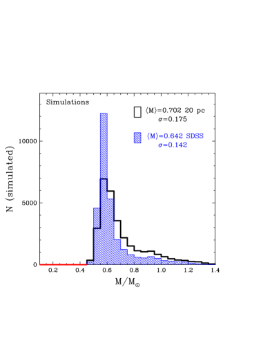
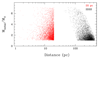
Fig. 7 shows the initial mass versus total age distribution for white dwarfs in our simulated samples. The 20 pc sample covers a large range of initial parameters, but our SDSS sample has a dramatically different structure. The latter is limited to short-lived intermediate-mass stars ($2\lesssim M/M_{\odot}\lesssim 8$) formed in the last 1 Gyr and older stars ($1\lesssim M/M_{\odot}\lesssim 2$) that have just the right mass and age to have recently evolved from the main-sequence 20-200 Myr ago. The steepness of the main-sequence lifetime versus initial mass relation combined with white dwarf cooling ages lead to a very specific coverage of initial parameters in Fig. 7. When this is joined with the IMF, IMFR, and variation of vertical scale height as a function of stellar age, we can ultimately define the number of high mass white dwarfs. As a consequence, it is far from as simple as correcting for stellar radius bias.

The volume covered by our samples is shown in Fig. 8. Volume effects depend critically on the vertical scale height of the Galactic disk, which varies from 75 pc at 1 Gyr to 200 pc at 5 Gyr in our model. For both samples, this effect increases the number of high-mass white dwarfs in comparison to a constant scale height. Indeed, massive white dwarfs come from short-lived intermediate mass stars and have smaller total ages, hence a smaller average vertical scale height. For the 20 pc sample which is located close to the plane of the disk, it directly increases the number of high-mass white dwarfs. For our SDSS sample, massive white dwarfs have total ages of $\sim$1 Gyr according to Fig. 7, hence a vertical scale height of $\sim$75 pc. Fig. 8 demonstrates that our sample is sensitive to massive white dwarfs at distances of $\sim$50-150 pc, hence we maximize their numbers by having a vertical scale height in the same range.

Figure 7: Initial mass as a function of total stellar age for white dwarfs simulated in the 20 pc (top) and SDSS samples (bottom, $16,000<T_{\rm eff}$ (K) $<22,000$ and $16.0<g<18.5$). There are 5000 simulated objects in both samples.

Figure 8: Initial mass as a function of the distance to the Sun (logarithmic scale) for white dwarfs simulated in the 20 pc (red) and SDSS samples (black, $16,000<T_{\rm eff}$ (K) $<22,000$ and $16.0<g<18.5$). There are 5000 simulated objects in both samples.

One important finding of this work is that the mean masses of the 20 pc and SDSS white dwarf samples are predicted to be significantly different. We predict a 9% larger mean mass for the 20 pc sample, while observations in Fig. 1 and Fig. 4 show an offset of 10%. We therefore suggest that this observed difference in mean mass is largely caused by the structure of the samples, and not due to a systematic difference between the photometric and spectroscopic techniques, which are the dominant methods to determine the atmospheric parameters for the 20 pc and SDSS samples, respectively. We defer to Section 5 the detailed comparison of the observed mass distributions and simulations.

4 Review of Uncertainties

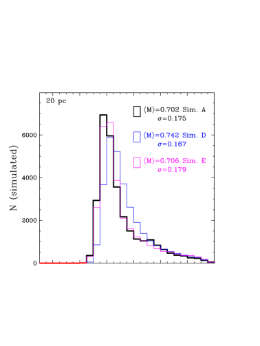
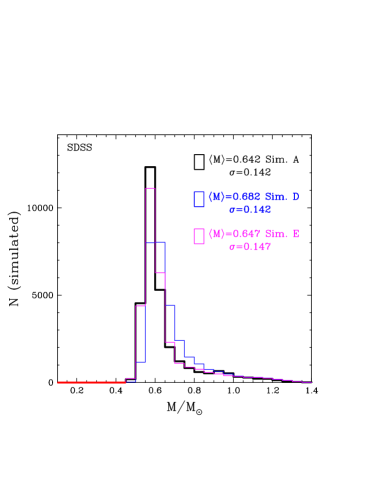
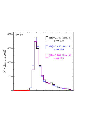
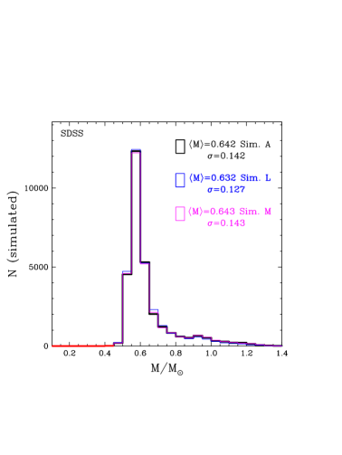
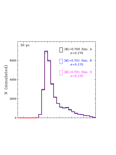
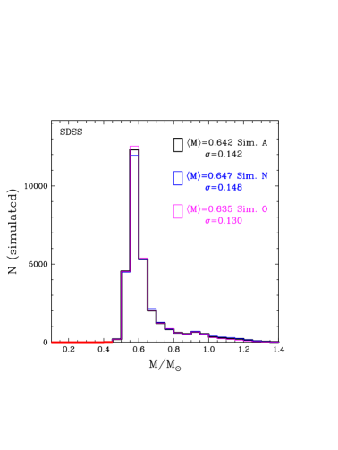
We now review in turn various uncertainties and biases that impact the simulated mass distributions. As a summary of these experiments, we present in Table 2 the mean mass, mass dispersion, and fraction of high-mass white dwarfs for the observations and all numerical experiments (which we label from $A$ to $P$). The fraction of high-mass white dwarfs is defined as the fraction of objects with $M/M_{\odot}>0.75$ with respect to the full considered range ($M/M_{\odot}>0.45$). For both surveys, the observed fraction of massive remnants is too small compared to the predictions of our standard simulations. This is in line with the preliminary assessment of Tremblay et al. (2014) who found that the 20 pc mass distribution appeared significantly steeper than the Salpeter IMF. For the 20 pc and SDSS samples, the observed number of massive white dwarfs would need to increase by a factor of 1.42 and 1.54, respectively, to match the simulations.

Table 2: Observed Mass Distributions and Monte Carlo Simulations

		20 pc sample			SDSS sample
ID	Data	$\langle M\rangle$	$\sigma_{\rm M}$	N$(>0.75M_{\odot})$	$\langle M\rangle$	$\sigma_{\rm M}$	N$(>0.75M_{\odot})$	Reference
		($M_{\odot})$	($M_{\odot})$	%	($M_{\odot})$	($M_{\odot})$	%
$...$	Observed	0.680	0.130	20.6	0.619	0.108	10.0	Sect. 2, Figs. 1 and 4
A	Standard Monte Carlo	0.702	0.175	26.9	0.642	0.142	14.6	Sect. 3, Figs. 1 and 4
B	$V<17$ (20 pc only)	0.687	0.162	24.3	$-$	$-$	$-$	Sect. 4.1, Fig. 9
C	No observational errors	0.701	0.171	26.3	0.642	0.140	14.6	Sect. 4.2, Fig. 9
D	Kalirai et al. 2008 IFMR	0.742	0.167	35.5	0.682	0.142	20.1	Sect. 4.3, Fig. 10
E	Cummings et al. 2016a IFMR (linear)	0.706	0.179	27.0	0.647	0.147	15.2	Sect. 4.3, Fig. 10
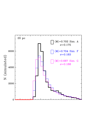
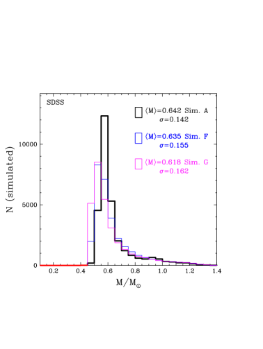
F	Catalán et al. 2008 IFMR	0.704	0.183	29.2	0.635	0.155	16.4	Sect. 4.3, Fig. 11
G	Casewell et al. 2009 IFMR	0.687	0.188	27.1	0.618	0.162	15.5	Sect. 4.3, Fig. 11
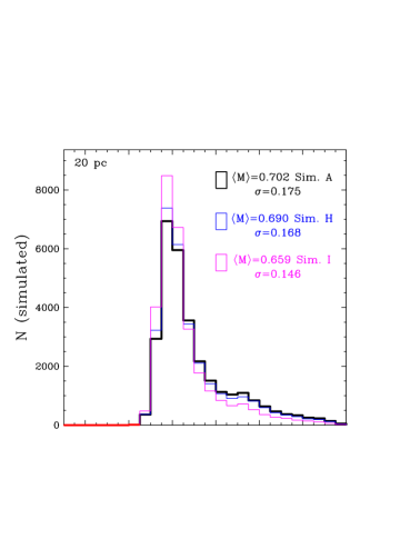
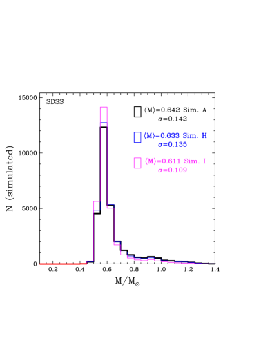
H	IMF $\alpha=2.5$	0.690	0.168	24.7	0.633	0.135	12.7	Sect. 4.4, Fig. 12
I	IMF $\alpha=3.0$	0.659	0.146	17.5	0.611	0.109	8.1	Sect. 4.4, Fig. 12
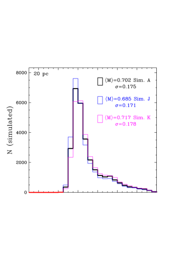
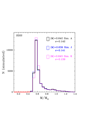
J	Constant SFH in last 12 Gyr	0.685	0.171	23.8	0.639	0.141	14.2	Sect. 4.5, Fig. 13
K	Tremblay et al. 2014 SFH	0.717	0.178	29.8	0.643	0.139	13.9	Sect. 4.5, Fig. 13
L	No vertical scale height variation	0.685	0.168	23.1	0.632	0.127	12.5	Sect. 4.6, Fig. 14
M	Thick H-layers only	0.701	0.175	26.8	0.643	0.143	14.9	Sect. 4.7, Fig. 14
N	Salaris et al. 2010 cooling models	0.701	0.175	26.8	0.647	0.148	15.5	Sect. 4.7, Fig. 15
O	O/Ne-cores for $M_{\rm WD}>1.05M_{\odot}$	0.701	0.175	27.0	0.635	0.130	13.6	Sect. 4.7, Fig. 15
P	Removal of magnetic WDs (SDSS only)	$-$	$-$	$-$	0.639	0.139	14.0	Sect. 4.9, Fig. 16
Notes. The different Monte Carlo experiments ($A$ to $P$) are described throughout this work. The standard case $A$ includes observational errors, a Salpeter IMF ($\alpha=2.35$), a constant SFH in the last 10 Gyr, the velocity dispersion versus total age relation of Eqs. 1-2, a 2nd order fit of the Cummings et al. (2016a) IFMR defined in Eqs. 3-4, and the C/O-core cooling models of Fontaine et al. (2001). We neglect low-mass objects ($M<0.45~{}M_{\odot}$) for the computation of the mean masses and mass dispersions and this should be taken into account when comparing to other studies.

Table 3: SDSS Mass Distribution

	Observed			Simulated
Data	$\langle M\rangle$	$\sigma_{\rm M}$	N$(>0.75M_{\odot})$	$\langle M\rangle$	$\sigma_{\rm M}$	N$(>0.75M_{\odot})$
	($M_{\odot})$	($M_{\odot})$	%	($M_{\odot})$	($M_{\odot})$	%
22,000 $<T_{\rm eff}$ (K) $<$ 30,000	0.599	0.109	6.4	0.665	0.166	20.6
16,000 $<T_{\rm eff}$ (K) $<$ 22,000	0.619	0.108	10.0	0.642	0.142	14.6
12,000 $<T_{\rm eff}$ (K) $<$ 16,000	0.643	0.100	10.8	0.647	0.139	16.1
8000 $<T_{\rm eff}$ (K) $<$ 12,000	0.636	0.106	12.5	0.649	0.129	16.8
Notes. The observations include DA and DB white dwarfs for $T_{\rm eff}>$ 16,000 K but only DAs for smaller temperatures.

4.1 Selection Effects

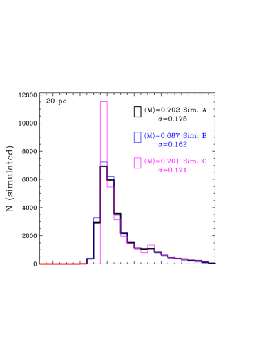
This section discusses completeness issues regarding single white dwarfs, while effects from missing white dwarfs in binaries are reviewed in Section 4.8. The 20 pc sample is only 80-90% complete, hence missing objects could impact the mass distribution if they tend to be fainter and more massive than the average. To test this scenario, we have a added a magnitude cutoff of $V<17$ to our simulation $B_{\rm 20pc}$ in Fig. 9. This removes nearly 7% of the sample and brings the mean mass down by about 0.01 $M_{\odot}$ according to Table 2. It confirms that objects at the faint end are significantly more massive than the average. Yet, this magnitude cutoff is largely insufficient to bring the fraction of high-mass white dwarfs in agreement with the observations. Gaia will substantially improve the completeness by detecting most white dwarfs in the local sample down to $V\sim 20$.

One interesting finding of this work is that about 2% of all local degenerate stars, corresponding to about 2 objects within 20 pc, are massive white dwarfs within the so-called ultra-cool regime, i.e. with temperatures well below 4000 K. For $M_{\rm WD}\sim 1.0$ $M_{\odot}$, a star that formed 10 Gyr ago spent a negligible amount of time on the main-sequence and is now a 4000 K white dwarf. As the mass further increases, it takes less and less time to cool to 4000 K. For $M_{\rm WD}=1.2$ $M_{\odot}$, all stars formed more than 7 Gyr ago are now massive ultracool white dwarfs, some of them with temperatures well below 2000 K. We find that this interpretation remains valid even when employing alternative cooling models (see Section 4.7), including O/Ne-core cooling tracks. While not of immediate concern for this work, it will become an important issue for the definition of halo white dwarf samples in the Gaia and Euclid era.

We have already studied the selection effects for the SDSS sample in Section 2. Another way to confirm our results is to select different $T_{\rm eff}$ subsamples and compare to our standard case. Table 3 presents the comparison between observations and simulations for different $T_{\rm eff}$ regimes. From experiments similar to the one presented in Fig. 3, we have verified that the spectroscopic completeness does not change significantly as a function of mass over the $T_{\rm eff}$ ranges identified in Table 3. However, the completeness as a function of $T_{\rm eff}$ is not constant. Furthermore, masses for non-DA white dwarfs are not available for $T_{\rm eff}<16,000$ K. Nevertheless, Table 3 demonstrates that the high-mass fraction is overpredicted at all temperatures.

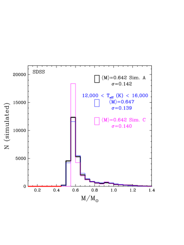
Fig. 9 shows that the predicted SDSS mass distribution in the range $12,000<T_{\rm eff}$ (K) $<16,000$ is fairly similar to our warmer standard case. It is difficult to predict mean mass variations as a function of $T_{\rm eff}$ since it depends significantly on the variation of the vertical scale height as a function of total stellar age. Indeed, distances for the magnitude-limited SDSS sample are strongly correlated with $T_{\rm eff}$ values. As a consequence, the variations in the simulated mean masses presented in Table 3 should be taken as indicative only.

The observations also show mean mass fluctuations as a function of temperature according to Table 3. They are thought to be caused by spectroscopic calibration issues (Kleinman et al., 2004; Tremblay et al., 2011), and to a lesser degree missing subtypes as well as incomplete 3D effects (Tremblay et al., 2013). The data calibration issues were first discussed for the SDSS DR1 sample (Kleinman et al., 2004) and the status appears largely unchanged in our analysis employing the DR10 reduction. In the $16,000<T_{\rm eff}$ (K) $<22,000$ regime of our standard sample, the SDSS spectra lead to lower derived masses compared to independent observations (see, e.g., Gianninas et al., 2011). An account of this bias would generate a better agreement between the observations and our standard SDSS simulation.

Figure 9: Comparison of our standard Monte Carlo simulations $A$ (thick black lines) with alternative experiments for the 20 pc (top panel) and SDSS (bottom) samples. Case $B$ is with a faint magnitude limit of $V<17$ (20 pc sample only) and case $C$ neglects observational mass errors in both panels. For the SDSS sample, we show the distribution for 12,000 $<T_{\rm eff}$ (K) $<$ 16,000, which contrasts with our standard case in the range 16,000 $<T_{\rm eff}$ (K) $<$ 22,000. There are 30,000 simulated objects for both samples.

4.2 Observational Errors

Most white dwarfs are formed close to the $\sim$0.6 $M_{\odot}$ peak and the observed shape of that peak is largely determined by how it is convolved with observational errors. This effect is confirmed by Case $C$ in Fig. 9 where we have removed observational errors. However, there is only a small impact on the mean mass, the fraction of high-mass objects, and even the mass dispersion. Nevertheless, it demonstrates that it would be necessary to perform a more careful assessment of the observational errors, possibly including asymmetries, to properly fit the observed white dwarf mass distributions with a grid of Monte Carlo simulations.

4.3 Initial-Final Mass Relation

The IFMR relation is clearly a critical parameter to map the IMF into the white dwarf mass distribution (Catalán et al., 2008). While the intermediate-mass IFMR is relatively well understood (see, e.g., Cummings et al., 2015), the slope at the low-mass end, roughly defined as $M_{\rm WD}<0.65$ $M_{\odot}$ ($M_{\rm i}\lesssim 2.5$ $M_{\odot}$), is still poorly constrained (Catalán et al., 2008; Kalirai et al., 2008, 2009; Zhao et al., 2012). This has a crucial impact on the simulated mass distributions since the mass peak is well within this regime. Furthermore, the high-mass end of the IMFR ($M_{\rm WD}>1.0$ $M_{\odot}$) is also poorly explored since massive white dwarfs are rare in clusters (Williams et al., 2009; Cummings et al., 2016a, b; Raddi et al., 2016), and one has to rely on an extrapolation to predict the high-mass tail of the simulated mass distributions.

Figs. 10 and 11 present our results with a set of four alternative IFMRs, all of them linear relations. For cases $D$, $E$, $F$, and $G$, respectively, we employ the relation of Kalirai et al. (2008), the results of Cummings et al. (2016a) as used in our standard case but with a linear instead of a two-part 2nd order fit, the parameterisation of Catalán et al. (2008), and the IFMR from Casewell et al. (2009). As expected, these alternative assumptions have a strong impact on the predicted mass distributions. For both samples, the mean mass varies by as much as $\sim$0.06 $M_{\odot}$, while the fraction of massive white dwarfs changes by up to 8%. It is therefore clear that the low- and high-mass regimes of the IFMR must be better understood to predict the field white dwarf mass distribution. However, all of our assumed IFMRs predict a too large amount of massive white dwarfs, suggesting it is unlikely to be the only source of the discrepancy.

Figure 10: Similar to Fig. 9 but with alternative numerical experiments. Case $D$ employs the IFMR of Kalirai et al. (2008) and case $E$ uses a linear fit to the Cummings et al. (2016a) IFMR. For the standard case $A$ we rely on a two-part 2nd order fit to the Cummings et al. (2016a) IFMR.

Figure 11: Similar to Fig. 9 but with alternative numerical experiments. Case $F$ relies on the IFMR of Catalán et al. (2008) and case $G$ uses the relation from Casewell et al. (2009).

4.4 Initial Mass Function

We have repeated our simulations with a steeper IMF. Instead of the Salpeter relation, we have employed $\alpha$ = 2.5 and 3.0 in cases $H$ and $I$, respectively. The results are shown in Fig. 12. For both samples, Table 2 suggests that an IMF slightly steeper than $\alpha$ = 2.5 would put the mean mass, mass dispersion, and massive white dwarf fraction in fairly good agreement with the observations. We note that Weisz et al. (2015) find a high-mass IMF of $\alpha$ = 2.45${}^{+0.03}_{-0.06}$ from young clusters in M31. Furthermore, Bochanski et al. (2010) have used SDSS data to derive a low-mass single star IMF (0.32 $<M_{\rm i}/M_{\odot}<0.8$) that is consistent with $\alpha\sim$ 2.60. Our results at face value also suggest a single star IMF steeper than Salpeter for the disk of the Milky Way in the range 1.0 $<M_{\rm i}/M_{\odot}<8.0$. It is however difficult to isolate the effect of the IMF from other input parameters.

Figure 12: Similar to Fig. 9 but with alternative numerical experiments. We employ an IMF with a power index of $\alpha=2.5$ for case $H$ and $\alpha=3.0$ for case $I$, while the standard case uses the Salpeter value of $\alpha=2.35$.

4.5 Stellar Formation History

Our standard case assumes a constant SFH for the Galactic disk in the last 10 Gyr. Fig. 13 presents the results supposing instead an age of 12 Gyr for the disk. The effect is quite important for the 20 pc sample as it greatly enhances the number of $\sim$1 $M_{\odot}$ stars that became white dwarfs. The effect on the SDSS mass distribution of young white dwarfs is much smaller. While it is clear that our experiment overestimates the age of the disk (see, e.g., Winget et al., 1987), it illustrates that one has to obtain a precise estimate of this parameter to model the field white dwarf mass distribution.

We have recently constrained the local SFH from white dwarfs within 20 pc (Tremblay et al., 2014). We have not used this result so far since the technique employed to derive the SFH is more sensitive at intermediate ages ($\sim$3-10 Gyr) and constraints on the last 2 Gyr depend much more on the assumed IMF. In particular, for the SDSS sample where most massive white dwarfs are from stars formed in the last 1 Gyr, it is difficult to apply our earlier SFH results. Nevertheless, Fig. 13 presents the case $K$ where we have used the white dwarf determined SFH from Tremblay et al. (2014) instead of a constant value. The impact on the mass distributions is moderate. Our input SFH peaks at 2-4 Gyr and Fig. 7 shows that no massive SDSS white dwarf is found in that range, resulting in a smaller high-mass fraction for that sample. It is the opposite situation for the 20 pc sample where the high-mass fraction increases. There is currently no consensus on the SFH and radial migration within the Galactic disk (see, e.g., Tremblay et al., 2014). As a consequence, it is difficult to quantify the amplitude and sign of this bias.

Figure 13: Similar to Fig. 9 but with alternative numerical experiments. For case $J$ we employ an age of 12 Gyr instead of 10 Gyr for the Galactic disk and case $K$ uses the SFH derived in Tremblay et al. (2014) instead of a constant formation rate.

4.6 Vertical Scale Height of the Galactic Disk

Previous studies of white dwarf luminosity functions have often assumed a constant vertical scale height of 250 pc for the Galactic disk (see, e.g., Harris et al., 2006; Torres & García-Berro, 2016). It is nonetheless known that cooler white dwarfs have a larger vertical ($W$) velocity dispersion. From the Sion et al. (2014) kinematic analysis of the 25 pc sample, it is possible to divide the sample for cooling ages below and above 1.37 Gyr ($T_{\rm eff}\sim 8000$ K) and conclude that the older bin has a larger vertical velocity dispersion by a factor of $\sim$1.5. If we do the same analysis for our standard local sample simulation, we find a ratio of 1.4-1.9 depending on the Galactic disk model used to transform scale height into velocity dispersion. This suggests that our scale height variation model drawn from main-sequence star observations is appropriate. Nevertheless, there are very few studies that constrain the absolute values of the vertical scale height of white dwarfs and one should be cautious with the predictions of our standard simulations.

Fig. 14 shows the case $L$ where we assume a constant vertical scale height of 250 pc for the Galactic disk. This alternative parameterisation has significant consequences since high-mass white dwarfs are now formed at much higher Galactic latitudes on average. For both the SDSS and 20 pc samples, Fig. 7 shows that most massive degenerates are detected close to the plane of disk where the Sun is located. This reduces the simulated fractions of massive white dwarfs as seen in Table 2, in better agreement with the observations. Lower mass white dwarfs are relatively unaffected since they already have a scale height of $\sim$200 pc in our standard simulations owing to their large total ages on average. Nevertheless, it appears unrealistic that the vertical scale height is constant or decrease with time, hence it is unlikely that it is the main reason for the overprediction of massive white dwarfs.

Figure 14: Similar to Fig. 9 but with alternative numerical experiments. We assume that the vertical scale height of the Galactic disk has a constant value of 250 pc in case $L$ and that all white dwarfs have thick H-layers instead of 70% with thick and 30% with thin H-layers in case $M$.

4.7 White Dwarf Models and Evolution Tracks

For case $M$, we have used thick hydrogen layers for all objects and Fig. 14 demonstrates that the effect is negligible compared to other biases. Additionally, we have employed alternative cooling sequences from Salaris et al. (2010) in case $N$, where effects of C/O phase separation and sedimentation are taken into account. We have also used Althaus et al. (2007) evolutionary sequences with O/Ne cores for $M_{\rm WD}>1.05$ $M_{\odot}$ in case $O$. Fig. 15 demonstrates that changes are small for both experiments. Regarding the high-mass fraction, the effects on the 20 pc sample are negligible since the cooling rates do not change the distance or membership. For the SDSS sample, we note that O/Ne cores reduce the number of high-mass white dwarfs, in the direction of bringing the simulations in better agreement with the observations.

Further uncertainties lie in the model atmospheres and fitting techniques used to extract the observed mass distributions. For instance, Fig. 2 shows the overall SDSS mass distribution for the same DR7 sample of DA white dwarfs, but with spectroscopic masses determined by two independent studies. The differences are moderate, and most often not significant for a single spectrum, but still lead to systematic effects on the mean mass and high-mass fraction.

Figure 15: Similar to Fig. 9 but with alternative numerical experiments. We employ the cooling sequences of Salaris et al. (2010) for C/O-core white dwarfs in case $N$ and O/Ne-core evolutionary sequences from Althaus et al. (2007) for $M_{\rm WD}>1.05$ $M_{\odot}$ in case $O$.

4.8 Binaries

We have so far neglected unresolved binaries both in our simulations and observed distributions. That includes WD+MS and WD+WD binaries, where WD stands for white dwarf and MS for main-sequence. We discuss merger products separately in Section 5.1.

The fraction of WD+MS binaries as function of initial mass is likely to vary strongly and binarity appears to be more common in massive stars (Kouwenhoven et al., 2009), hence high-mass white dwarfs. Such scenario is difficult to constrain from white dwarf populations because we have little information on the unbiased mass distribution of white dwarfs in binaries. Increasing the fraction of binaries as a function of initial mass would be similar to using a steeper single star IMF for our single white dwarf simulations. This would make our simulations in better agreement with the observations.

Our cutoff below 0.45 $M_{\odot}$ should eliminate most He-core white dwarfs formed through binary evolution. However, post-common envelope binaries also include C/O-core white dwarfs (see, e.g., Rebassa-Mansergas et al., 2011; Camacho et al., 2014). Some of these systems are likely present in our sample when the companion is an unseen low-mass star or a white dwarf. In those cases, the brighter and lower mass white dwarf will likely have suffered mass loss. Accounting for this effect would bring our simulations in closer agreement with the observations.

Finally, double degenerates that have not previously interacted could also be a problem since the lower mass white dwarf will dominate the flux and massive white dwarf companions could be hidden. Tremblay et al. (2011) find a $\sim$1% fraction of DA+DB/DC double degenerates in the SDSS, suggesting a five times larger DA+DA fraction given that the ratio of hydrogen to helium atmospheres is about 5/1 (Kleinman et al., 2013). Only a small number of those are expected to have large mass ratios, suggesting that double degenerates may not significantly impact the observed mass distributions.

4.9 Magnetic White Dwarfs

Magnetic white dwarfs in the 20 pc sample are included in the observed mass distribution of Fig. 1 because they have precise masses from trigonometric parallax measurements. On the other hand, we have neglected magnetic white dwarfs from the observed SDSS distribution since there are no mass estimates for them. We have identified 2.5% of magnetic DA white dwarfs in our revised analysis of the SDSS DR7 sample. We can account for these objects by assuming that the same fraction of our simulated white dwarfs are magnetic. It is suggested that the mass distribution for magnetic degenerates peaks around $\sim$0.8 $M_{\odot}$ (Briggs et al., 2015; Ferrario et al., 2015). We note that the 15 magnetic degenerates in our 20 pc sample have a mean mass of 0.75 $M_{\odot}$, which is 11% larger than the non-magnetic white dwarfs. As a consequence, we assume that the probability of an object being magnetic varies linearly with mass. The slope and amplitude of this function are fixed to obtain a mean mass of 0.8 $M_{\odot}$ and a magnetic fraction of 2.5%. Finally, we have removed those magnetic objects in case $P$ presented in Fig.16. The impact is to reduce the mean mass and high-mass fraction, though the effect is moderate given the small total number of magnetic white dwarfs. We mention that if these magnetic white dwarfs come from mergers, our simulations do not adequately represent them.

Figure 16: Similar to Fig. 9 but for the alternative numerical experiment $P$ (SDSS only) where we have removed the contribution from a population of magnetic white dwarfs with an incidence of 2.5% and a mean mass of 0.80 $M_{\odot}$.

5 Discussion

The white dwarf mass distributions from the 20 pc and SDSS samples were first studied by designing Monte Carlo simulations with fixed standard astrophysical constraints. The good qualitative agreement between simulations and observations in Figs. 1 and 4 confirms that the local white dwarf population is consistent with our basic knowledge of stellar and Galactic evolution. We have then systematically studied the uncertainties on the input parameters of the simulations. Our results suggest that given our current knowledge of stellar and Galactic evolution, we can only predict the mean mass and mass dispersion of observed samples within $\sim$10%. Additionally, we find that the relative number of high-mass white dwarfs ($M>0.75$ $M_{\odot}$) can only be predicted within a factor of $\sim$1.5. The main uncertainties are the assumed IFMR and the IMF, followed by the SFH, the scale height variation of the Galactic disk as a function total stellar age, and binaries. Other biases lead to moderate changes, such as effects from missing magnetic white dwarfs (SDSS sample), incompleteness (20 pc sample), white dwarf model atmospheres and evolution tracks, and core composition. Finally, we find that observational errors lead to fairly small uncertainties on the mean properties and high-mass fraction.

From the same local white dwarf sample as the one studied in this work, Tremblay et al. (2014) have successfully extracted the local SFH in the last 10 Gyr. We have verified that if we observe our Monte Carlo simulation $K_{\rm 20pc}$ with added observational errors, we can recover the input SFH from Tremblay et al. (2014) to a high precision with the technique described in that work. Our present study does not lessen the significance of this recent determination of the SFH in the solar neighborhood. We demonstrate instead that it is difficult to extract the IMF from the same sample. The first reason for this behaviour is that Tremblay et al. (2014) have used a direct method employing both the mass and cooling age of individual white dwarfs. In the present case, we consider the mass distribution integrated over all ages. The second reason why it is difficult to constrain the IMF is that the IMFR leads to similar effects on the mass distribution. Finally, biases owing to binary populations and incompleteness directly impact the mass distributions, while Tremblay et al. (2014) have demonstrated that it does not lead to significant systematic effects on the SFH.

We find that our simulations overpredict the fraction of massive white dwarfs by a factor of $\sim$1.5 for both the 20 pc and SDSS samples. This interpretation is consistent with earlier Monte Carlo simulations of similar populations (see, e.g., Catalán et al., 2008). This result suggests a single star IMF that is significantly steeper than Salpeter for the Galactic disk. However, if we account for all uncertainties, a Salpeter IMF is not ruled out. We note that this result differs from the common view that there is an observed excess of massive white dwarfs when representing the peak in the mass distributions with a Gaussian function (see, e.g., Kleinman et al., 2013). We do not challenge this fact but only the astrophysical interpretation. Our calculations suggest that Gaussian functions are a poor substitute to realistic simulations including stellar and Galactic evolution when attempting to understand the nature of high-mass white dwarfs.

Gaia will soon provide precise parallaxes for all white dwarfs studied in this work. This will supply precise independent masses leading to a better understanding of the observed mass distributions. Gaia will also provide a much better picture of the completeness of the samples. For the SDSS sample in particular, this includes the identification of double degenerates and the determination of precise masses for all subtypes including magnetic white dwarfs. By identifying a much larger 40 pc sample with the help of Gaia and spectroscopic follow-ups, it will be possible to improve our understanding of the local SFH and kinematics as a function of age and mass. For instance, it will be possible to study the mass distribution for subsamples in total age, reducing the uncertainties due to Galactic evolution effects. Nevertheless, it could remain a challenge to disentangle the effects from the IMF and IFMR on the mass distribution even with the Gaia data, although many more white dwarfs in clusters and common proper motion pairs will be discovered allowing to improve the IFMR. Our study will be useful to re-assess all uncertainties in the Gaia era.

5.1 Constraining the Merger Population

Little is known about the fraction of white dwarfs that are the product of mergers (WD+WD, WD+RG, or RG+RG, where RG stands for red giant) in the solar neighborhood. Wegg & Phinney (2012) have analysed the kinematics of massive SDSS white dwarfs and demonstrated that they have the characteristics of a young singly-evolved population. From multi-epoch spectroscopy of SDSS white dwarfs, Badenes & Maoz (2012) have calculated the WD+WD merger rate to be around $1.4\times 10^{-13}$ yr${}^{-1}M_{\odot}^{-1}$. Binary population synthesis models predict merger rates that are about twice as large (Iben et al., 1997; Toonen et al., 2012). For the last 10 Gyr, this leads to approximately one merger product in our main SDSS subsample in the range $16,000<T_{\rm eff}$ (K) $<$ 22,000. On the other hand, this does not include stars that have merged before both of them became white dwarfs (WD+RG or RG+RG), which could account for a larger fraction. However, there is little evidence that a merging process involving red giants would favour the production of white dwarfs that are more massive than the average (García-Berro et al., 2012).

On the other hand, early investigations of the white dwarf mass distribution have identified a high-mass peak or so-called bump around 0.8 $M_{\odot}$ (Marsh et al., 1997; Vennes, 1999), and proposed a merger population as a possible cause. More recently, Giammichele et al. (2012) and Kleinman et al. (2013) have also suggested that the high-mass peak is likely due to mergers. However, these studies are not based on extensive simulations of stellar populations, which for instance Kleinman et al. (2013) are cautious to mention. Nevertheless, Giammichele et al. (2012) suggests that mergers account for $\sim$3% of the 20 pc sample. This is much larger than the observed WD+WD merger rate.

From the simulations performed in this work, we can suggest a number of alternatives to explain features in the field white dwarf mass distribution. First of all, our standard set of simulations already predict too many massive white dwarfs. Hence there is no need to invoke mergers to explain even the most massive (non-magnetic) white dwarfs in the current samples. This applies to the SDSS mass distribution at all temperatures according to Table 3. Furthermore, even our standard simulations have a bump around 0.8 $M_{\odot}$, and this is most easily seen when we neglect observational errors in Fig. 9. This feature is in fact due to the two-piece polynomial fit to the IFMR of Cummings et al. (2016a). It is not present when using any linear IFMR. We do not claim that it is a real astrophysical feature of the IFMR even though our parameterisation was motivated by theoretical IMFRs (Cummings et al., 2016a). It merely demonstrates that current constraints on single star evolution and the IFMR do not rule out the presence of a high-mass peak. Finally, there are number of biases that impact the field white dwarf mass distribution, the combination of which could cause the high-mass peak. We conclude that no evidence of WD+WD mergers can be found in the field white dwarf mass distribution.

6 Conclusions

We have presented a thorough study on the astrophysical interpretation of the field white dwarf mass distribution. We have chosen the well studied 20 pc and SDSS samples, restricting the latter to $16,000<T_{\rm eff}$ (K) $<$ 22,000, $16<g<18.5$, and single non-magnetic white dwarfs in order to have a well understood completeness. Our approach has been to perform Monte Carlo simulations to compare with the observations. The first result of this work is that we predict a larger mean mass for the 20 pc sample in comparison to the SDSS sample, in agreement with the observations. This suggests that the photometric technique and model atmospheres of cool white dwarfs, largely employed for the local sample, are in agreement with the results of the spectroscopic technique for hotter DA and DB white dwarfs is the SDSS.

Our simulations reproduce reasonably well the samples studied in this work using standard assumptions about stellar and Galactic evolution. However, for both samples our simulations predict too many high-mass white dwarfs ($M>0.75$ $M_{\odot}$) by a factor of $\sim$1.5. From our extensive review of biases that impact our simulations, we find that this offset is not unexpected. Probable causes are uncertainties in the assumed IFMR, IMF, SFH, variation of Galactic disk vertical scale height as a function of total stellar age, binary evolution, neglect of magnetic white dwarfs (SDSS), and unidentified faint massive objects (20 pc sample). While a majority of these uncertainties will be improved with Gaia, it could remain a challenge to disentangle the effects from the IFMR and IMF.

Our results challenge the interpretation that there is evidence for a population of WD+WD mergers in the field white dwarf mass distribution. On the contrary, we find no observed excess of high-mass objects and features in the observed distributions can not be unambiguously linked to mergers. We note that our results do not rule out a population WD+MS or WD+WD mergers that are not preferentially massive, or that some percentage of known massive single white dwarfs, e.g. with large magnetic fields, could be directly linked to a merger event.

References

- Alam et al. (2015) Alam, S., Albareti, F. D., Allende Prieto, C., et al. 2015, ApJS, 219, 12
- Althaus et al. (2007) Althaus, L. G., García-Berro, E., Isern, J., Córsico, A. H., & Rohrmann, R. D. 2007, A&A, 465, 249
- Badenes & Maoz (2012) Badenes, C., & Maoz, D. 2012, ApJ, 749, L11
- Bastian et al. (2010) Bastian, N., Covey, K. R., & Meyer, M. R. 2010, ARA&A, 48, 339
- Bergeron et al. (1992) Bergeron, P., Saffer, R. A., & Liebert, J. 1992, ApJ, 394, 228
- Bergeron et al. (2011) Bergeron, P., Wesemael, F., Dufour, P., et al. 2011, ApJ, 737, 28
- Bochanski et al. (2010) Bochanski, J. J., Hawley, S. L., Covey, K. R., et al. 2010, AJ, 139, 2679
- Briggs et al. (2015) Briggs, G. P., Ferrario, L., Tout, C. A., Wickramasinghe, D. T., & Hurley, J. R. 2015, MNRAS, 447, 1713
- Buckner & Froebrich (2014) Buckner, A. S. M., & Froebrich, D. 2014, MNRAS, 444, 290
- Camacho et al. (2014) Camacho, J., Torres, S., García-Berro, E., et al. 2014, A&A, 566, A86
- Catalán et al. (2008) Catalán, S., Isern, J., García-Berro, E., & Ribas, I. 2008, MNRAS, 387, 1693
- Carrasco et al. (2014) Carrasco, J. M., Catalán, S., Jordi, C., et al. 2014, A&A, 565, A11
- Casewell et al. (2009) Casewell, S. L., Dobbie, P. D., Napiwotzki, R., et al. 2009, MNRAS, 395, 1795
- Chabrier (2003) Chabrier, G. 2003, PASP, 115, 763
- Cojocaru et al. (2015) Cojocaru, R., Torres, S., Althaus, L. G., Isern, J., & García-Berro, E. 2015, A&A, 581, A108
- Conroy et al. (2010) Conroy, C., White, M., & Gunn, J. E. 2010, ApJ, 708, 58
- Cummings et al. (2015) Cummings, J. D., Kalirai, J. S., Tremblay, P.-E., & Ramirez-Ruiz, E. 2015, ApJ, 807, 90
- Cummings et al. (2016a) Cummings, J. D., Kalirai, J. S., Tremblay, P.-E., & Ramirez-Ruiz, E. 2016a, ApJ, 818, 84
- Cummings et al. (2016b) Cummings, J. D., Kalirai, J. S., Tremblay, P.-E., Ramirez-Ruiz, E., & Bergeron, P. 2016b, ApJ, 820, L18
- Daddi et al. (2007) Daddi, E., Dickinson, M., Morrison, G., et al. 2007, ApJ, 670, 156
- Dan et al. (2015) Dan, M., Guillochon, J., Brüggen, M., Ramirez-Ruiz, E., & Rosswog, S. 2015, MNRAS, 454, 4411
- De Gennaro et al. (2008) De Gennaro, S., von Hippel, T., Winget, D. E., et al. 2008, AJ, 135, 1
- Dobbie et al. (2012) Dobbie, P. D., Day-Jones, A., Williams, K. A., et al. 2012, MNRAS, 423, 2815
- Ferrario et al. (2005) Ferrario, L., Wickramasinghe, D., Liebert, J., & Williams, K. A. 2005, MNRAS, 361, 1131
- Ferrario et al. (2015) Ferrario, L., de Martino, D., Gänsicke, B. T. 2015, Space Sci. Rev., 191, 111
- Fontaine et al. (2001) Fontaine, G., Brassard, P., & Bergeron, P. 2001, PASP, 113, 409
- García-Berro et al. (2012) García-Berro, E., Lorén-Aguilar, P., Aznar-Siguán, G., et al. 2012, ApJ, 749, 25
- Gentile Fusillo et al. (2015) Gentile Fusillo, N. P., Gänsicke, B. T., & Greiss, S. 2015, MNRAS, 448, 2260
- Gianninas et al. (2011) Gianninas, A., Bergeron, P., & Ruiz, M. T. 2011, ApJ, 743, 138
- Giammichele et al. (2012) Giammichele, N., Bergeron, P., & Dufour, P. 2012, ApJS, 199, 29
- Harris et al. (2006) Harris, H. C., Munn, J. A., Kilic, M., et al. 2006, AJ, 131, 571
- Holberg et al. (2008) Holberg, J. B., Sion, E. M., Oswalt, T., et al. 2008, AJ, 135, 1225
- Hurley et al. (2000) Hurley, J. R., Pols, O. R., & Tout, C. A. 2000, MNRAS, 315, 543
- Iben et al. (1997) Iben, I. Jr., Tutukov, A. V., & Yungelson, L. R. 1997, ApJ, 475, 291
- Isern et al. (2013) Isern, J., Catalán, S., García-Berro, E., & Hernanz, M. 2013, in 18th European White Dwarf Workshop, ASP Conference Proceedings, ed. J. Krzesiński, G. Stachowski, P. Moskalik, & K. Bajan (San Francisco, ASP), 469, 71
- Kalirai et al. (2007) Kalirai, J. S., Bergeron, P., Hansen, B. M. S., et al. 2007, ApJ, 671, 748
- Kalirai et al. (2008) Kalirai, J. S., Hansen, B. M. S., Kelson, D. D., et al. 2008, ApJ, 676, 594
- Kalirai et al. (2009) Kalirai, J. S., Saul Davis, D., Richer, H. B., et al. 2009, ApJ, 705, 408
- Kalirai et al. (2014) Kalirai, J. S., Marigo, P., & Tremblay, P.-E. 2014, ApJ, 782, 17
- Kepler et al. (2016) Kepler, S. O., Pelisoli, I., Koester, D., et al. 2016, MNRAS, 455, 3413
- Koester & Kepler (2015) Koester, D., & Kepler, S. O. 2015, A&A, 583, A86
- Kouwenhoven et al. (2009) Kouwenhoven, M. B. N., Brown, A. G. A., Goodwin, S. P., Portegies Zwart, S. F., & Kaper, L. 2009, A&A, 493, 979
- Kleinman et al. (2004) Kleinman, S. J., Harris, H. C., Eisenstein, D. J., et al. 2004, ApJ, 607, 426
- Kleinman et al. (2013) Kleinman, S. J., Kepler, S. O., Koester, D., et al. 2013, ApJS, 204, 5
- Kroupa et al. (1993) Kroupa, P., Tout, C. A., & Gilmore, G. 1993, MNRAS, 262, 545
- Lam et al. (2015) Lam, M. C., Rowell, N., & Hambly, N. C. 2015, MNRAS, 450, 4098
- Laureijs et al. (2011) Laureijs, R., Amiaux, J., Arduini, S., et al. 2011, arXiv:1110.3193
- Liebert et al. (2005) Liebert, J., Bergeron, P., & Holberg, J. B. 2005, ApJS, 156, 47
- Maraston (2005) Maraston, C. 2005, MNRAS, 362, 799
- Marigo & Girardi (2007) Marigo, P., & Girardi, L. 2007, A&A, 469, 239
- Marsh et al. (1997) Marsh, M. C., Barstow, M. A., Buckley, D. A., et al. 1997, MNRAS, 287, 705
- Meng et al. (2008) Meng, X., Chen, X., & Han, Z. 2008, A&A, 487, 625
- Raddi et al. (2016) Raddi, R., Catalán, S., Gänsicke, B. T., et al. 2016, MNRAS, 457, 1988
- Rebassa-Mansergas et al. (2011) Rebassa-Mansergas, A., Nebot Gómez-Morán, A., Schreiber, M. R., Girven, J., Gänsicke, B. T. 2011, MNRAS, 413, 1121
- Rebassa-Mansergas et al. (2015) Rebassa-Mansergas, A., Rybicka, M., Liu, X.-W., Han, Z., & García-Berro, E. 2015, MNRAS, 452, 1637
- Rowell (2013) Rowell, N. 2013, MNRAS, 434, 1549
- Salaris et al. (2010) Salaris, M., Cassisi, S., Pietrinferni, A., Kowalski, P. M., & Isern, J. 2010, ApJ, 716, 1241
- Salpeter (1955) Salpeter, E. E. 1955, ApJ, 121, 161
- Seabroke & Gilmore (2007) Seabroke, G. M., & Gilmore, G. 2007, MNRAS, 380, 1348
- Sion et al. (2009) Sion, E. M., Holberg, J. B., Oswalt, T. D., McCook, G. P., & Wasatonic, R. 2009, AJ, 138, 1681
- Sion et al. (2014) Sion, E. M., Holberg, J. B., Oswalt, T. D., et al. 2014, AJ, 147, 129
- Spitzer (1942) Spitzer, L. 1942, ApJ, 95, 329
- Toonen et al. (2012) Toonen, S., Nelemans, G., & Portegies Zwart, S. 2012, A&A, 546, A70
- Toonen & Nelemans (2013) Toonen, S., & Nelemans, G. 2013, A&A, 557, A87
- Torres et al. (2014) Torres, S., García-Berro, E., Krzesinski, J., & Kleinman, S. J. 2014, A&A, 563, A47
- Tout et al. (2004) Tout, C. A., Wickramasinghe, D. T., & Ferrario, L. 2004, MNRAS, 355, L13
- Tout et al. (2008) Tout, C. A., Wickramasinghe, D. T., Liebert, J., Ferrario, L., & Pringle, J. E. 2008, MNRAS, 387, 897
- Tremblay & Bergeron (2008) Tremblay, P.-E., & Bergeron, P. 2008, ApJ, 672, 1144
- Tremblay et al. (2011) Tremblay, P.-E., Bergeron, P., & Gianninas, A. 2011, ApJ, 730, 128
- Tremblay et al. (2013) Tremblay, P.-E., Ludwig, H.-G., Steffen, M., & Freytag, B. 2013, A&A, 559, A104
- Tremblay et al. (2014) Tremblay, P.-E., Kalirai, J. S., Soderblom, D. R., Cignoni, M., & Cummings, J. 2014, ApJ, 791, 92
- Torres & García-Berro (2016) Torres, S., & García-Berro, E. 2016, arXiv:1602.02533
- Verbeek et al. (2013) Verbeek, K., Groot, P. J., Nelemans, G., et al. 2013, MNRAS, 434, 2727
- Vennes (1999) Vennes, S. 1999, ApJ, 525, 995
- Weidemann (2000) Weidemann, V. 2000, A&A, 363, 647
- Weisz et al. (2015) Weisz, D. R., Johnson, L. C., Foreman-Mackey, D., et al. 2015, ApJ, 806, 198
- Wegg & Phinney (2012) Wegg, C., & Phinney, E. S. 2012, MNRAS, 426, 427
- Wickramasinghe et al. (2014) Wickramasinghe, D. T., Tout, C. A., & Ferrario, L. 2014, MNRAS, 437, 675
- Williams et al. (2009) Williams, K. A., Bolte, M., & Koester, D. 2009, ApJ, 693, 355
- Winget et al. (1987) Winget, D. E., Hansen, C. J., Liebert, J., et al. 1987, ApJ, 315, L77
- Zhao et al. (2012) Zhao, J. K., Oswalt, T. D., Willson, L. A., Wang, Q., & Zhao, G. 2012, ApJ, 746, 144