Partial redistribution in 3D non-LTE radiative transfer in solar atmosphere models

Abstract

Context. Resonance spectral lines such as H I Ly $\alpha$, Mg II h&k, and Ca II H&K that form in the solar chromosphere are influenced by the effects of 3D radiative transfer as well as partial redistribution (PRD). So far no one has modeled these lines including both effects simultaneously owing to the high computing demands of existing algorithms. Such modeling is however indispensable for accurate diagnostics of the chromosphere.

Aims. We present a computationally tractable method to treat PRD scattering in 3D model atmospheres using a 3D non-LTE radiative transfer code.

Methods. To make the method memory-friendly, we use the hybrid approximation of Leenaarts et al. (2012b) for the redistribution integral. To make it fast, we use linear interpolation on equidistant frequency grids. We verify our algorithm against computations with the RH code and analyze it for stability, convergence, and usefulness of acceleration using model atoms of Mg II with the h&k lines and H I with the Ly $\alpha$ line treated in PRD.

Results. A typical 3D PRD solution can be obtained in a model atmosphere with $252\times 252\times 496$ coordinate points in 50 000–200 000 CPU hours, which is a factor ten slower than computations assuming complete redistribution. We illustrate the importance of the joint action of PRD and 3D effects for the Mg II h&k lines for disk-center intensities as well as the center-to-limb variation.

Conclusions. The proposed method allows simulating PRD lines in time series of radiation-MHD models in order to interpret observations of chromospheric lines at high spatial resolution.

1 Introduction

At the beginning of the development of radiative transfer theory, astrophysicists assumed that scattering in spectral lines is coherent. This assumption is however unable to reproduce observed intensity profiles and their center-to-limb variation in detail. In the 1940s, a better approximation called complete frequency redistribution (CRD) was introduced. Houtgast (1942) validated it using systematic observations of various line profiles in the solar spectrum.

The CRD approximation means that during line scattering there is no correlation between absorbed and emitted photons. CRD requires atomic levels of the line transition to be strongly perturbed by elastic collisions with other atoms. This is true in dense layers of stellar atmospheres such as the photosphere of the Sun. With a few exceptions, all lines visible in the solar spectrum are formed in CRD. The CRD approximation makes the line source function constant, which strongly simplifies analytical and numerical solutions of the radiative transfer problem in such lines.

In the 1970s, as reviewed by Linsky (1985) and Nagirner (1987), it became clear that strong chromospheric lines actually demonstrate partially-coherent scattering (nowadays more commonly referred to as partial frequency redistribution, PRD). Although the theory of PRD was developed earlier, only then it became possible to model PRD lines due to high computational demands for the redistribution functions.

Contrary to CRD, PRD includes the fact that photon scattering is not arbitrary and could even be fully correlated in the most extreme case of coherent scattering. Line scattering becomes partially or fully coherent only if several conditions are met together (Hubeny & Mihalas 2014, see p. 519). The upper atomic level of the line transition must be weakly perturbed by elastic collisions to be able to retain radiatively-excited sublevels during the finite radiative lifetime of the level. This is true in low-density layers of stellar atmospheres such as the chromosphere of the Sun. The chemical element of the line has to be abundant and exist in a dominant ionization stage so that the line extinction dominate over the continuum extinction by several orders of magnitude. The line has to be a resonance transition, or a transition whose lower level is metastable

Only a small number of lines in the solar spectrum are affected by PRD but they are indispensable as diagnostics of the outer atmosphere of the Sun. Among them are: the strongest lines of H I Lyman series such as the Ly $\beta$ 102.6 nm and the Ly $\alpha$ 121.6 nm lines (Milkey & Mihalas 1973; Hubený & Lites 1995); the strongest chromospheric Mg II k 279.6 nm and h 280.4 nm (Milkey & Mihalas 1974) as well as the Ca II K 393.4 nm and H 396.8 nm lines (Vardavas & Cram 1974; Shine et al. 1975); strong resonance UV lines of abundant neutrals such as the Mg I 285.2 nm line (Canfield & Cram 1977) or the O I resonance triplet at 130 nm (Miller-Ricci & Uitenbroek 2002); and resonance lines of other alkali and alkaline-earth metals such as the Na I D 589 nm doublet or the Ba II 455.4 nm line, which are mostly formed in the photosphere but show PRD effects towards the extreme limb (Uitenbroek & Bruls 1992; Babij & Stodilka 1993; Rutten & Milkey 1979).

In the chromosphere, where PRD lines are formed, the 3D spatial transport of radiation becomes essential (Leenaarts et al. 2009, 2010, 2012a; Štěpán et al. 2015; Judge et al. 2015). So far no one has modeled PRD lines including the effects of 3D non-LTE radiative transfer due to the large computational effort that is required.

In this paper, we present a method to perform 3D non-LTE radiative transfer with PRD effects, which was implemented in the Multi3D code (Leenaarts & Carlsson 2009), and investigate whether such modeling is significant. We are motivated to make up for a lack of accurate physical models needed to interpret observations in the Mg II h&k lines from the IRIS satellite (De Pontieu et al. 2014), measurements in the H I Ly $\alpha$ line obtained by the CLASP rocket experiment (Kubo et al. 2014), and observations in the Ca II H&K lines using the new imaging spectrometer CHROMIS at the Swedish 1-m Solar Telescope.

The structure of the paper is as follows. Section 2 briefly explains the method to solve the 3D non-LTE radiative transfer problem in PRD lines. Section 3 describes the computational setup: model atmospheres, model atoms, and the code. Section 4 lays out the most important computational specifics. Section 5 presents the results for our calculations, which we verify, analyze for stability, convergence speed, and applicability of acceleration. Using intensities computed in the Mg II h&k lines, we illustrate the importance of 3D non-LTE radiative transfer with PRD effects. In Section 6, we give some conclusions. Technical details on the algorithm are given in Appendix A.

2 Method

The iterative solution algorithm of Multi3D employs preconditioning of the rate equations as formulated by Rybicki & Hummer (1991, 1992). This method was extended by Uitenbroek (2001) to include the effects of PRD and implemented in the RH code, the de facto standard for non-LTE radiative transfer calculations in plane-parallel geometry. The RH code has been extended to allow for parallel computation of a large number of plane-parallel atmospheres (1.5D approximation) by Pereira & Uitenbroek (2015). Below we briefly review the algorithm and the extension by Leenaarts et al. (2012b), who devised a method to compute a fast approximate solution of the full angle-dependent PRD problem in moving atmospheres.

2.1 The PRD algorithm in the Rybicki-Hummer framework

The statistical equilibrium non-LTE radiative transfer problem for an atom with $N_{\mathrm{L}}$ levels consists of solving the rate equations for the atomic level populations:

$$\dfrac{\mathrm{d}n_{i}}{\mathrm{d}t}=\sum_{j,\,j\neq i}^{N_{\mathrm{L}}}n_{\!j}P_{\!ji}-n_{i}\sum_{j,\,j\neq i}^{N_{\mathrm{L}}}P_{i\!j}=0,$$ (1)

with $n$ the atomic level populations, and $P_{i\!j}=C_{i\!j}+R_{i\!j}$ the total rates consisting of collisional rates $C_{i\!j}$ and radiative rates $R_{i\!j}$. The radiative rates depend on the specific intensity $I(\@vec{n},\nu)$, which in turn depends on the direction $\@vec{n}$ and the frequency $\nu$, and is computed from the transfer equation:

$$\frac{\mathrm{d}I(\@vec{n},\nu)}{\mathrm{d}s}=j(\@vec{n},\nu)-\alpha(\@vec{n},\nu)\,I(\@vec{n},\nu).$$ (2)

The transfer equation couples different locations in the atmosphere and makes the problem non-linear and non-local.

The assumption of complete redistribution (CRD) is that the frequency and direction of the absorbed and emitted photon in a scattering event are uncorrelated, so that the normalized emission profile $\psi_{\!ji}(\@vec{n},\nu)$ and absorption profile $\varphi_{\!ji}(\@vec{n},\nu)$ in a transition $i{\to}j$ are equal:

$$\psi_{\!ji}(\@vec{n},\nu)=\varphi_{\!ji}(\@vec{n},\nu),$$ (3)

for all frequencies $\nu$ and directions $\@vec{n}$. If PRD is important then this equality is no longer valid, and following Uitenbroek (1989) we define:

$$\rho_{i\!j}(\@vec{n},\nu)\equiv\frac{\psi_{\!ji}(\@vec{n},\nu)}{\varphi_{i\!j}(\@vec{n},\nu)}.$$ (4)

The profile ratio $\rho_{i\!j}(\@vec{n},\nu)$ describes for the transition $i{\to}j$ how strongly the line emissivity correlates with the line opacity for the direction $\@vec{n}$ and the frequency $\nu$. It depends on the local particle densities, temperature and the local radiation field $I(\@vec{n},\nu)$. It is discussed in more detail in Section 2.2. The contributions into the opacity and emissivity from the PRD transition $i{\to}j$ are

$$\alpha_{i\!j}(\@vec{n},\nu) =\frac{h\nu}{4\pi}B_{i\!j}\varphi_{i\!j}(\@vec{n},\nu)\biggl{[}n_{i}-n_{\!j}\frac{g_{i}}{g_{\!j}}\rho_{i\!j}(\@vec{n},\nu)\biggr{]}\quad\text{and}$$ (5)

$$j_{i\!j}(\@vec{n},\nu) =\frac{h\nu}{4\pi}A_{\!ji}\varphi_{i\!j}(\@vec{n},\nu)\Bigl{[}n_{\!j}\rho_{i\!j}(\@vec{n},\nu)\Bigr{]},$$ (6)

with $n$ and $g$ the corresponding level populations and statistical weights, and $A_{\!ji}$, $B_{\!ji}$, and $B_{i\!j}$ the Einstein coefficients. This means that the line source function

$$S_{\!i\!j}(\@vec{n},\nu)=\frac{n_{\!j}A_{\!ji}\rho_{i\!j}(\@vec{n},\nu)}{n_{i}B_{i\!j}-n_{\!j}B_{\!ji}\rho_{i\!j}(\@vec{n},\nu)}=\frac{2h\nu^{3}}{c^{2}}\biggl{[}\frac{1}{\rho_{i\!j}(\@vec{n},\nu)}\frac{n_{i}}{n_{\!j}}\frac{g_{\!j}}{g_{i}}-1\biggr{]}^{-1}$$ (7)

depends on frequency and direction, in contrast to CRD where it is constant.

The radiative rates in the PRD transition $i{\to}j$ are

$$R_{i\!j} =B_{i\!j}\bar{J}_{i\!j}^{\varphi}\quad\text{and}$$ (8)

$$R_{\!ji} =A_{\!ji}+B_{\!ji}\bar{J}_{\!ji}^{\psi},$$ (9)

where the mean angle-averaged intensities integrated with the absorption and emission profiles are denoted by

$$\bar{J}_{\!i\!j}^{\varphi} \equiv\oint\mspace{-11.0mu}\int\!I(\@vec{n},\nu)\,\varphi_{i\!j}(\@vec{n},\nu)\,\mathrm{d}\nu\,\frac{\mathrm{d}\Omega}{4\pi}\quad\text{and}$$ (10)

$$\bar{J}_{\!\!ji}^{\psi} \equiv\oint\mspace{-11.0mu}\int\!I(\@vec{n},\nu)\,\psi_{i\!j}(\@vec{n},\nu)\,\mathrm{d}\nu\,\frac{\mathrm{d}\Omega}{4\pi}.$$ (11)

The Rybicki-Hummer method of solving the non-LTE problem in PRD consists of the following conceptual steps:

1. The level populations are initialized with a guess solution. Popular choices are LTE populations, or populations based on assuming a zero radiation field, or a previously computed solution assuming CRD.

2. The profile ratios $\rho_{i\!j}(\@vec{n},\nu)$ are initalized to unity for each PRD transition $i{\to}j$.

3. The formal solution of the radiative transfer equation is performed for all directions and frequencies to obtain intensities.

4. Using the resulting intensities a preconditioned set of rate equations is formulated.

5. The solution of the preconditioned equations gives an improved estimate of the true solution for the level populations.

6. A number of extra PRD sub-iterations are performed, where the level populations are kept fixed and only intensity is redistributed:

   1. The formal solution is computed again only for the frequencies in the PRD transitions.

   2. Using the new intensities, the redistribution integral is computed in each PRD transition to update the profile ratio $\rho_{i\!j}(\@vec{n},\nu)$.

   3. Using the new profile ratio, line opacities and emissivities are updated.

   4. Steps (a)–(c) are repeated until the changes to the radiation field are smaller than a desired value.

7. From $\rho_{i\!j}(\@vec{n},\nu)$ updated opacities and emissivities are computed.

8. Steps 3-7 are repeated until convergence.

For more details we refer the reader to Uitenbroek (2001) and Rybicki & Hummer (1991, 1992).

2.2 The profile ratio $\rho_{i\!j}(\@vec{n},\nu)$

The core of the PRD scheme is the calculation of the redistribution integrals to compute the profile ratio $\rho_{i\!j}(\@vec{n},\nu)$. Following Uitenbroek (1989), we consider the PRD transition $i{\to}j$ with all subordinate transitions $k{\to}j\colon k<j$, which share the same broadened upper level $j$. The redistribution integrals, computed in each subordinate transition $k{\to}j$ including the transition $i{\to}j$ itself then contribute into the profile ratio:

$$\rho_{i\!j}(\@vec{n},\nu)=1+\sum_{k<j}\dfrac{n_{k}B_{k\!j}}{n_{\!j}P_{\!j}}\\ {\times}\oint\mspace{-11.0mu}\int\!\!I\bigl{(}\@vec{n}^{\prime}\!,\nu^{\prime}\bigr{)}\Biggl{[}\frac{R_{k\!ji}\bigl{(}\@vec{n}^{\prime}\!,\nu^{\prime}\!;\@vec{n},\nu\bigr{)}}{\varphi_{i\!j}(\@vec{n},\nu)}-\varphi_{k\!j}\bigl{(}\@vec{n}^{\prime}\!,\nu^{\prime}\bigr{)}\Biggr{]}\mathrm{d}\nu^{\prime}\frac{\mathrm{d}\Omega^{\prime}\!}{4\pi},$$ (12)

with $R_{k\!ji}$ the inertial-frame redistribution function, $P_{\!j}=\sum_{k\neq j}P_{\!jk}$ the total depopulation rate out of the upper level $j$, where each double redistribution integral is taken over photons with frequencies $\nu^{\prime}\!$ coming along directions $\@vec{n}^{\prime}$ within solid angles $\Omega^{\prime}$ that are absorbed in the subordinate lines $k{\to}j$ including the resonance transition $i{\to}j$.

As the inertial frame redistribution function $R_{k\!ji}$ we use a function for transitions with a sharp lower level and a broadened upper level, which is generalised for two possible cascades of a normal redistribution in the $i{\to}j{\to}i$ transition itself and resonance Raman scattering (also called cross-redistribution) in $k{\to}j{\to}i\colon k\neq i$ subordinate transitions sharing the same upper level $j$. The function $R_{k\!ji}$ consists of two weighted components (Hubený 1982):

$$R_{k\!ji}\bigl{(}\@vec{n}^{\prime}\!,\nu^{\prime}\!;\@vec{n},\nu\bigr{)}=\gamma R_{k\!ji}^{\mathrm{II}}\bigl{(}\@vec{n}^{\prime}\!,\nu^{\prime}\!;\@vec{n},\nu\bigr{)}+(1-\gamma)\varphi_{k\!j}\bigl{(}\@vec{n}^{\prime}\!,\nu^{\prime}\bigr{)}\varphi_{i\!j}\bigl{(}\@vec{n},\nu\bigr{)}.$$ (13)

Here $R_{k\!ji}^{\mathrm{II}}$ is the inertial frame correlated redistribution function for a transition with a sharp lower level and a broadened upper level, representing coherent scattering. The product $\varphi_{k\!j}\varphi_{i\!j}$ approximates the inertial frame non-correlated redistribution function $R_{k\!ji}^{\mathrm{III}}$, representing complete redistribution. The quantity $\gamma\equiv P_{\!j}/\bigl{(}P_{\!j}+Q_{\!j}^{\mathrm{E}}\bigr{)}$ is the coherence fraction, i.e., the ratio of total rate $P_{\!j}$ out of level $j$ to its sum with the rate of elastic collisions $Q_{\!j}^{\mathrm{E}}$. Entering (13) into (12) we finally obtain

$$\rho_{i\!j}(\@vec{n},\nu)=\\ 1+\gamma\!\sum_{k<j}\frac{n_{k}B_{k\!j}}{n_{\!j}P_{\!j}}\left[\oint\mspace{-11.0mu}\int\!\!I\bigl{(}\@vec{n}^{\prime}\!,\nu^{\prime}\bigr{)}\frac{R_{k\!ji}^{\mathrm{II}}\bigl{(}\@vec{n}^{\prime}\!,\nu^{\prime}\!;\@vec{n},\nu\bigr{)}}{\phi_{i\!j}(\@vec{n},\nu)}\mathrm{d}\nu^{\prime}\frac{\mathrm{d}\Omega^{\prime}\!}{4\pi}-\bar{J}_{\!k\!j}^{\varphi}\right]$$ (14)

2.3 The hybrid approximation

Computing the profile ratio using Eq. (14) is computationally expensive, as it involves evaluating the angle-dependent redistribution function $R_{k\!ji}^{\mathrm{II}}/\varphi_{i\!j}$ and computing the double integral along each absorption frequency $\nu^{\prime}$ and direction $\@vec{n}^{\prime}$ for each emission frequency $\nu$ and direction $\@vec{n}$. Leenaarts et al. (2012b) demonstrated in plane-parallel computations using RH, that evaluating Eq. (14) takes about a factor 100 more time than computing the formal solution for all angles and frequencies.

A common additional assumption to speed up the computations is to assume that the radiation field $I(\@vec{n},\nu)$ is isotropic in the inertial frame. In that case the angle integral in Eq. (14) can be performed analytically to obtain

$$\rho_{i\!j}(\nu)=1+\gamma\!\sum_{k<j}\frac{n_{k}B_{k\!j}}{n_{\!j}P_{\!j}}\Biggl{[}\int\!\!J\bigl{(}\nu^{\prime}\bigr{)}\,\varg_{k\!ji}^{\mathrm{II}}\bigl{(}\nu^{\prime}\!,\nu\bigr{)}\,\mathrm{d}\nu^{\prime}\!-\bar{J}_{k\!j}^{\varphi}\Biggr{]}.$$ (15)

with an angle-averaged redistribution function $\varg_{k\!ji}^{\mathrm{II}}$ (e.g., Gouttebroze 1986; Uitenbroek 1989). The assumption of isotropy is not valid if the velocities in the model atmosphere are larger than the Doppler width of the absorption profile, a common situation in radiation-MHD simulations of the solar atmosphere (Magnan 1974; Mihalas et al. 1976).

Therefore Leenaarts et al. (2012b) proposed what they called the hybrid approximation, which is a fast and sufficiently accurate representation of Eq. (14) based on Eq. (15). The idea behind the hybrid approximation is to take the redistribution integral in the comoving frame assuming the radiation field to be isotropic there.

The angle-averaged intensity in the comoving frame $J^{\star\!}\bigl{(}\nu^{\star\!}\bigr{)}$ is computed from the intensity in the inertial frame $I(\@vec{n},\nu)$, taking into account Doppler shifts due to the local velocity $\@vec{\varv}$:

$$J^{\star\!}\bigl{(}\nu^{\star\!}\bigr{)}=\oint I\biggl{(}\@vec{n},\nu^{\star\!}\biggl{[}1+\frac{\@vec{n}\cdot\@vec{\varv}}{c}\biggr{]}\biggr{)}\frac{\mathrm{d}\Omega}{4\pi}.$$ (16)

The assumption of an isotropic specific intensity in the comoving frame $I^{\star\!}\bigl{(}\@vec{n},\nu^{\star\!}\bigr{)}=J^{\star\!}\bigl{(}\nu^{\star\!}\bigr{)}$ implies that we can use Eq. (15) with the angle-averaged redistribution function in the comoving frame to compute the comoving-frame profile ratio $\rho_{i\!j}^{\star}$ that depends only on frequency:

$$\rho_{i\!j}^{\star\!}\bigl{(}\nu^{\star\!}\bigr{)}=1+\gamma\!\sum_{k<j}\frac{n_{k}B_{k\!j}}{n_{\!j}P_{\!j}}\Biggl{[}\int\!\!J^{\star\!}\bigl{(}\nu^{\prime}\bigr{)}\,\varg_{k\!ji}^{\mathrm{II}}\bigl{(}\nu^{\prime}\!,\nu^{\star\!}\bigr{)}\mathrm{d}\nu^{\prime}\!-\bar{J}_{k\!j}^{\varphi}\Biggr{]},$$ (17)

where the integration is taken over the absorption frequency in the comoving frame. Finally, the comoving profile ratio $\rho_{i\!j}^{\star\!}$ is then transformed into the inertial profile ratio $\rho_{i\!j}$ using an inverse Doppler transform so that $\rho_{i\!j}$ again becomes dependent on both frequency and angle:

$$\rho_{i\!j}(\@vec{n},\nu)=\rho_{i\!j}^{\star\!}\biggl{(}\nu\biggl{[}1-\frac{\@vec{n}\cdot\@vec{\varv}}{c}\biggr{]}\biggr{)}.$$ (18)

Note that Eqs. (8)–(9) in Leenaarts et al. (2012b) contain two mistakes. First, both signs before $\@vec{n}\cdot\@vec{u}/c$ have to be inverted. Second, the subscript ‘r’ of $\nu_{\mathrm{r}}$ in Eq. (8) has to be dropped. We give the correct transforms here in Eqs. (16) and (18).

There are several different possibilities for numerically computing the interpolations in Eqs. (16) and (18). For Eq. (16), storing $I(\@vec{n},\nu)$ and then performing the interpolation and integration in one go is the most straightforward and rather fast. However, storing $I(\@vec{n},\nu)$ takes typically 1–4 GiB of memory per subdomain, which is too much on current-generation supercomputers, which normally have 2 GiB of memory per core (see the discussion in Sect. 4).

Another method is not to store the intensity, but instead to interpolate and incrementally add it to $J^{\star\!}$ during the formal solution. This method does not require as much storage, and we implemented various variants in Multi3D:

• General interpolation – interpolation indices and weights are computed on the fly. This method is slow but requires no additional storage.

• Precomputed interpolation – interpolation indices and weights are computed once, stored and then re-used. This method is fast, but requires a large memory storage.

• Interpolation on an equidistant frequency grid – this method is moderately fast, and requires only modest extra storage because the interpolation indices and weights depends only on the direction $\@vec{n}$ and not on frequency $\nu$.

We describe each of these algorithms in detail in Appendix A.

3 Computation setup

3.1 Model atmospheres

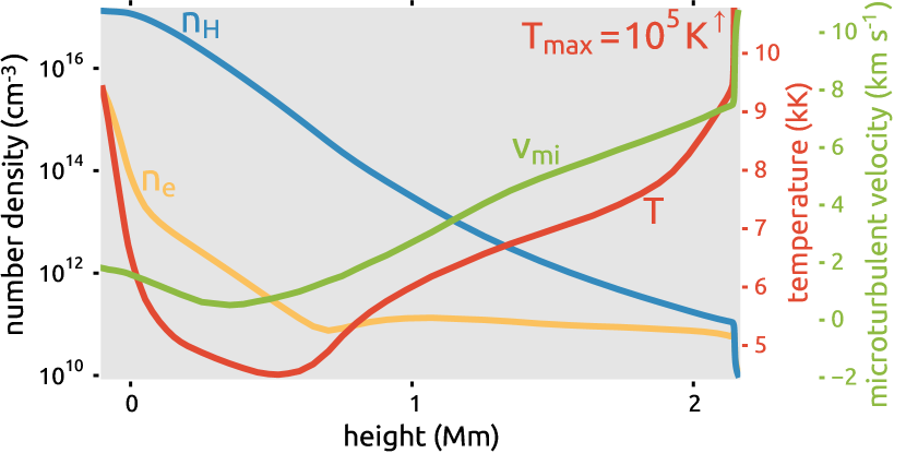
Figure 1: Height dependence of electron and hydrogen number densities, temperature, and velocities in the FAL-C (top) and the 1D Bifrost (bottom) model atmospheres. The vertical velocity is zero in the FAL-C model and the microturbulent velocity is zero in the 1D Bifrost model.

We tested our PRD algorithm using two different 1D model atmospheres with different velocity distributions. The standard FAL-C model atmosphere (Fontenla et al. 1993) shown in Fig. 1 (top) was modified to contain constant vertical velocities of ${-}10,\,0,\,{+}10$ km s^-1, two monotonically increasing from ${-}10$ to ${+}10$ km s^-1 and decreasing from ${+}10$ to ${-}10$ km s^-1 velocity gradients, two discontinuous velocity jumps from ${+}10$ to ${-}10$ km s^-1 and back representing toy shock waves, one smooth velocity composition of two waves with 10 and 6 km s^-1 amplitudes, and one random normal velocity distribution with a zero mean and a standard deviation of 10 km s^-1. Small insets in Fig. 4 illustrate some of these configurations. For timing, convergence stability, convergence acceleration, and other tests we employed a 1D column extracted from a radiation-MHD simulation performed with the Bifrost code (details given below). This column corresponds to coordinates $X=0$ and $Y=0$ of the original snapshot and is resampled into a vertical grid with 188 points in the Z-direction. Physical properties of this model atmosphere are illustrated in Fig. 1 (bottom). In this paper we simply refer to it as the 1D Bifrost model atmosphere.

To investigate how the algorithm performs in realistic situations, we used a snapshot from the 3D radiation-MHD simulation by Carlsson et al. (2016) corresponding to run time $t=3850$ s performed with the Bifrost code (Gudiksen et al. 2011). This snapshot contains a bipolar region of enhanced magnetic flux with unsigned field strength of 50 G in the photosphere. The simulation box spans from the bottom of the photosphere up to the corona having physical sizes of $24\times 24\times 16.8$ Mm. To save computational time, the horizontal resolution of the snapshot was halved to 96 km so that a new coarser grid with $252\times 252\times 496$ points is used. This snapshot has, amongst other studies, been used previously to study the formation of the hydrogen H$\alpha$ line (Leenaarts et al. 2012a), the Mg II h&k lines (Leenaarts et al. 2013b), and the C II lines (Rathore et al. 2015).

3.2 Model atoms

As a first test model atom we used a minimally sufficient model of Mg II with four levels and the continuum of Mg III, where first two resonance transitions represent the k 279.64 nm and h 280.35 nm doublet. Leenaarts et al. (2013a) provides more details on this $4{+}1$ level model atom.

As a second test model atom we used a model of H I with five levels and continuum of H II, where the first two resonance transitions represent the Ly $\alpha$ 121.6 nm and the Ly $\beta$ 102.6 nm lines.

For the timing experiments summarized in Table 2, we initialized all corresponding model atom transitions on a frequency grid of $N_{\nu}^{\mathrm{total}}$ points with $N_{\nu}^{\mathrm{PRD}}$ of them covered by PRD lines. PRD frequencies cover the two overlapping h&k lines for the Mg II model atom and by the Ly $\alpha$ line for the H I model atom.

3.3 Numerical code

We perform numerical simulations using an extensively updated version of the Multi3D code (Leenaarts & Carlsson 2009). The code solves the non-LTE radiative transfer problem for a given model atom in a given 3D model atmosphere using the method of short characteristics to integrate the formal solution of the transfer equation and the method of multilevel accelerated $\Lambda$-iterations (M-ALI) with pre-conditioned rates in the system of statistical equilibrium equations following Rybicki & Hummer (1991, 1992). The current version of the code allows MPI parallelization both for frequency and 3D Cartesian domains. A typical geometrical subdomain size is $32\times 32\times 32$ grid points. The code also employs non-overshooting 3rd order Hermite interpolation for the source function and the optical depth scale (Auer 2003; Ibgui et al. 2013). We use the 24-angle quadrature (A4 set) from Carlson (1963).

To treat resonance lines in PRD, we implemented non-coherent scattering into the code using the hybrid approximation with the three interpolation schemes mentioned in Sects. 2.1–2.2. We validate our Multi3D implementation with RH computations. In the RH code, the hybrid approximation for the PRD redistribution was implemented by Leenaarts et al. (2012b) for plane-parallel model atmospheres, and shown to give results consistent with full angle-dependent PRD.

4 Numerical considerations

4.1 Computational expenses of interpolation methods

We compared the time efficiency of each of the three interpolation methods mentioned in Sect. 2.3 using system clock routines in the computation of Eq. (16) (which we call forward transform) and Eq. (18) (which we call backward transform). Given a model atmosphere of $N_{\mathrm{X}}N_{\mathrm{Y}}N_{\mathrm{Z}}$ spatial grid points, using $N_{\mu}$ angles, and a frequency grid with $N_{\nu}$ knots, we computed the mean time spent per spatial point per ray direction per frequency for the forward transform ($t_{\blacktriangleright}$) and the backward transform ($t_{\blacktriangleleft}$). We also estimated how much memory each algorithm requires to store interpolation indices and weights. The numerical details of each interpolation method are given in Appendix A.

4.1.1 General interpolation

An advantage of the general interpolation algorithm is that it is applicable to any type of frequency grid with arbitrary spacing between knots and requires no memory storage for interpolation indices and weights. Drawbacks are that it is very time-consuming and it does not scale linearly with the number of grid points.

To perform the forward transform, for each knot in the inertial frame two full scans are done along knots in the comoving frame, resulting in $2N_{\nu}^{2}$ operations for the whole line profile. The mean time $t_{\blacktriangleright}$ spent per knot therefore scales as $O(N_{\nu})$.

To perform the backward transform, for each knot in the inertial frame a bisection search is done on the whole knot range in the comoving frame. The search can be correlated if the interpolation is performed along the frequency direction but this is not the case in Multi3D. The total number of operations is therefore around $2N_{\nu}\log_{2}N_{\nu}$ and $t_{\blacktriangleleft}$ scales as $O(\log_{2}N_{\nu})$.

4.1.2 Precomputed interpolation

The precomputed interpolation algorithm is applicable to any frequency grid, just like the general interpolation method. It is both very fast and scales well because interpolation indices and weights are computed only once based on the atmosphere, the chosen angles, and the frequency grid. The drawback is that the algorithm is memory consuming.

For each knot in the inertial frame two operations are performed for the forward transform, and thus $t_{\blacktriangleright}$ scales as $O(1)$.

In the backward transform, only one operation is done per inertial-frame knot, resulting in $t_{\blacktriangleleft}=O(1)$.

If we have a single non-overlapping PRD line (such as Ly $\alpha$), the forward transform requires storage of $3N_{\nu}N_{\mu}N_{\mathrm{X}}N_{\mathrm{Y}}N_{\mathrm{Z}}=3N_{\Sigma}$ numbers for interpolation indices and weights. For the backward transform, we need only $2N_{\Sigma}$ numbers (see Appendix A for details). For single-precision (4-byte) integers and floating point numbers this results in $20N_{\Sigma}$ bytes. For a typical run using the 3D model atmosphere we have $N_{\nu}\approx 200$, $N_{\mu}=24$, and a spatial subdomain size of $32^{3}$ grid points, so that storing the interpolation indices and weighs takes 2.9 GiB of memory per CPU. The data can be stored more efficiently by using less precise floating point numbers, so that the storage requirement is lowered to $14N_{\Sigma}$ bytes, corresponding to 2 GiB for our typical use case.

4.1.3 Precomputed interpolation on equidistant grid

The general interpolation algorithm is slow, and precomputed interpolation is fast but requires a large amount of memory. A solution to the memory consumption of the latter is to use an equidistant frequency grid, so that the interpolation weights and indices only depend on the ray direction and spatial grid point, but not on the frequency.

The requirement to properly sample to absorption profile sets the grid spacing to ${\sim}1$ km s^-1. Because PRD lines typically have wide wings, such sampling leads to thousands of knots. This is undesirable because of the corresponding increase in computing time.

It turns out that one can keep the advantages of an equidistant grid but not have the disadvantage of the low speed by performing the formal solution only for selected knots (which we call real). The other knots (which we call virtual) are ignored. We keep all knots real close to nominal line center in order to resolve the Doppler core, and have mainly virtual knots in the line wing where a coarse frequency resolution is acceptable. We can then still use frequency-independent interpolations coefficients, at the price of a small computational and memory overhead to track and store real and virtual knot locations and certain relations between them. Usually, $\sim$90 % of the real knots are in the line core.

The number of operations required to perform the forward transform depends on whether the real frequency knot is in the line core or in the line wings. The number of operations to perform the forward transform on all $N_{\nu}$ knots is around $2C_{\blacktriangleright}N_{\nu}$, where $1<C_{\blacktriangleright}\la 10$ is a factor that depends on $N_{\nu}$ and on the fine grid resolution. The $t_{\blacktriangleright}$ scales as $O(1)$ but the number of operations is higher than for precomputed interpolation.

In the backward transform, the algorithm is essentially the same. The total number of operations for all frequency knots is $2C_{\blacktriangleleft}N_{\nu}$, where $1<C_{\blacktriangleleft}<C_{\blacktriangleright}\la 10$ so that $t_{\blacktriangleleft}$ scales as $O(1)$.

The interpolation indices and weights are the same for both the forward and backward transforms. To store them we need $2N_{\mu}N_{\mathrm{X}}N_{\mathrm{Y}}N_{\mathrm{Z}}$ four-byte numbers resulting in 6 MiB plus some auxiliary variables amounting to another $0.3$ MiB.

4.1.4 Timing experiments

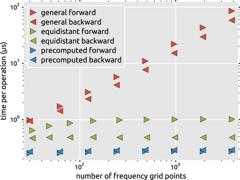
Figure 2: Dependence of the mean interpolation time spent per frequency per direction at spatial coordinate point on the total number of frequency points in one PRD line profile. Times are given for the forward ($\blacktriangleright$) and the backward ($\blacktriangleleft$) transforms for three different algorithms: general (red), precomputed (blue), and precomputed equidistant (green) interpolation. The measurements were done for the Mg II h&k lines in the 1D Bifrost model atmosphere.

We measured the performance of the three algorithms in the 1D Bifrost model atmosphere using the 5-level Mg II model atom with the two overlapping h&k lines treated in PRD. The number of frequency points in each line profile was varied from from 15 to 1 900. We used a ten-point Gauss-Legendre quadrature for the angle integrals. The calculations were run on a computer with Intel^® Xeon^® CPU E5-2697 v3 2.60 GHz cores.

Figure 2 shows our measurements for both transforms using the three interpolation algorithms. In the general algorithm, the total computing time scales as $O(N_{\nu}^{2})$ , which makes the algorithm unsuitable for wide chromospheric lines with many frequency points.

Contrary to that, the total time for the precomputed and the precomputed equidistant algorithms scales linearly as $O(N_{\nu})$. The equidistant algorithm is slower than the precomputed one, but of the same order. The extra book-keeping required for the equidistant interpolation causes a small performance penalty compared to the precomputed case. This is however a small price for the large saving in memory consumption compared to the precomputed algorithm.

We preferably use the precomputed algorithm in 1D and small 3D model atmospheres, while for big 3D model atmospheres we use the equidistant one.

4.2 Truncated frequency grid

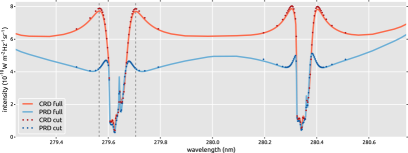
Figure 3: Intensity profiles of the Mg II h&k lines at $\mu_{\mathrm{Z}}=0.953$ computed on fully-winged (solid) or truncated (dots) frequency grids in CRD (red) or PRD (blue). Left: wide wavelength range showing both the k 279.6 nm and the h 280.3 nm lines. Dashed vertical lines show the wavelength range for the right panel. Right: close-up of the k line core. The model atmosphere is 1D Bifrost.

Only the core and inner wings of strong chromospheric lines are formed in the chromosphere, which is the region where observers of such lines are mainly interested in. It is therefore interesting to see whether ignoring the extended wings has an influence on the intensity in the central part of the line. If this is not the case we can lower the number of frequency points in the line profile and so speed up the computations.

Therefore we tested whether a truncation of the profile wings makes a difference. For the Mg II h&k lines, we performed a computation using equidistant interpolation where we resolve the core on a fine frequency grid up to $\pm 70$ km s^-1 around the line center, and use the coarse grid out to $\pm 160$ km s^-1, so that we only cover the core of the line profiles from just outside the h₁ and k₁ minima.

In Fig. 3 we show the differences between the truncated and the fully-winged profiles of the Mg II h&k lines in CRD and PRD. In CRD, there are small differences around the k₂ emission peaks while in PRD differences are negligible. We thus conclude that we can use a truncated grid.

The main reason why truncated grids work for chromospheric lines is that the density in the chromosphere is so low that the damping wings are weak, so that the extinction profile is well-approximated by a Gaussian. The averages over the extinction profile of the form

$$\oint\mspace{-11.0mu}\int\dotsi\varphi(\@vec{n},\nu)\,\mathrm{d}\nu\frac{\mathrm{d}\Omega}{4\pi}$$ (19)

that enter into the non-LTE problem are thus dominated by a range of few Doppler widths around the nominal line center in the local comoving frame. As long as the frequency grid covers this range, the radiative transfer in the chromosphere is accurate.

In CRD there is a larger inaccuracy because photons absorbed in the line wings tend to be re-emitted in the line core due to Doppler diffusion (Hubeny & Mihalas 2014). In PRD, this effect is weak, because the complete redistribution component of the redistribution function from Eq. (13) is strongly reduced because the coherency fraction $\gamma$ is nearly equal to one, so that the wings and the core are effectively decoupled and do not significantly influence each other. This is a rare instance where the inclusion of PRD effects actually makes computations easer instead of harder.

5 Results

5.1 Comparison to RH

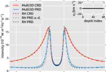
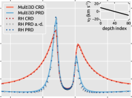
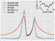
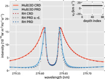
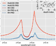
Figure 4: Intensity profiles of the Mg II h 279.64 nm line at $\mu_{\mathrm{Z}}=0.953$ computed using the Multi3D (solid) or the RH (dots) codes in CRD (red) or PRD (blue, white). PRD profiles are computed using either the hybrid approximation (blue) or full angle-dependent redistribution (white). The model atmosphere is FAL-C with modified vertical velocities. The profiles are shown for six different velocity configurations illustrated by the inset plots.

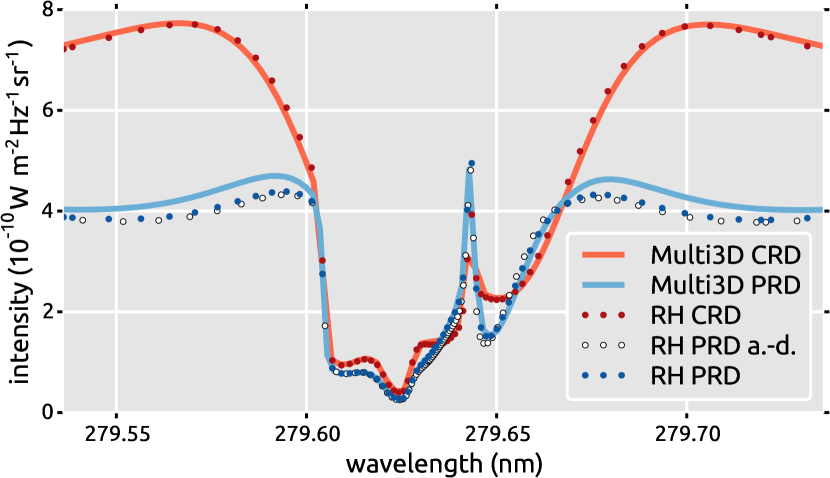
Figure 5: Same as in Fig. 4 but for the 1D Bifrost model atmosphere shown in Fig 1.

To validate our method and implementation, we simulated the Mg II h&k lines in CRD and PRD using both the Multi3D and the RH code, and compared the resulting intensities. The PRD calculations with RH were done using both the angle-dependent and the hybrid PRD algorithms, while Multi3D computations were done only using the hybrid algorithm.

Intensity profiles of both Mg II h&k lines were calculated in the FAL-C model atmosphere with modified vertical velocity distributions given in the insets in Fig. 4. The simplest cases are those with constant velocities, the most extreme is that with the random normal distribution. Note that the case of a random velocity distribution only illustrates that the method is stable in extreme situations.

Both codes produce CRD intensity profiles in a good agreement. Comparison of the RH computations using the hybrid and angle-dependent algorithms shows that the hybrid algorithm is accurate for all cases except the strong toy-shock wave. In such strong gradients the assumption of isotropy of the radiation in the comoving frame is not accurate.

Both codes yield the same hybrid PRD intensities except for some small differences around the inner wings close to the line core (see PRD intensity values at 279.58–279.61 nm and 279.65–279.68 nm in Fig. 4). This effect is caused by slight differences in frequency grids used by the codes and differences in line broadening recipes that lead to differences in coherency fraction $\gamma$.

We performed the same computations for the 1D Bifrost column. Corresponding profiles are given in Fig. 5. Also here both codes and algorithms yield excellent agreement.

5.2 Convergence properties

Numerical PRD operations are computationally expensive. In order to minimize the computing time we investigated how many PRD subiterations are needed to lead to a converged solution, how the number of subiterations influences the convergence speed of the ALI iterations, and whether convergence acceleration using the Ng method (Ng 1974) can be applied.

5.2.1 Number of PRD subiterations

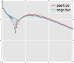
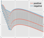
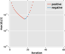
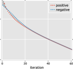
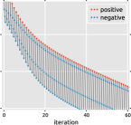
Figure 6: Iteration behavior of the maximum absolute relative change in mean intensity ($\max|\delta J/J|$) for the 5-level Mg II model atom with the k and the h lines treated in PRD in the FAL-C model atmosphere. Initial level populations are initialized to LTE populations (top row) or initialized using the zero radiation approximation (bottom row). Red markers indicate a positive $\max\delta J/J$, and blue markers a negative value. Grey lines connect values of successive PRD subiterations within one ALI-iteration. The number of PRD subiterations ranges from one to four (panels from left to right).

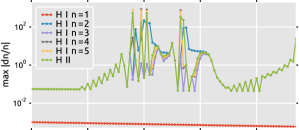
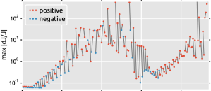
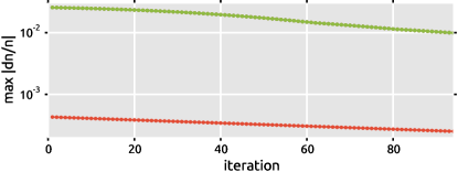
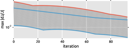
Figure 7: Iteration behavior of the maximum absolute relative changes in atomic level population $\max|\delta n/n|$ (left) and in angle-averaged intensity $\max|\delta J/J|$ (right) in the 3D Bifrost model atmosphere for the 6-level hydrogen model atom with the Ly $\alpha$ line treated in PRD. The top row shows the behavior with two subiterations, the bottom row with three subiterations. Note that the $\max|\delta n/n|$ values for the excited states of H I and the H II continuum overlap.

Table 1: Number of accelerated $\Lambda$-iterations needed to converge to a $\max|\delta n/n|\leq 10^{-4}$ solution against the number of PRD subiterations for different model atoms, model atmospheres, and approximations for initial atomic level populations.

model atmosphere:		FAL-C		1D Bifrost
initial populations:		LTE	zero radiation	LTE	zero radiation
		5-level Mg II
PRD subiterations	¿1	–	–	–	–
	¿2	168	124	695	438
	¿3	167	123	694	437
		6-level H I
PRD subiterations	¿1	–	–	–	–
	¿2	247	141	922	532
	¿3	247	140	917	526

We tested the convergence of accelerated $\Lambda$-iterations (ALI) for the Mg II and the H I model atoms with PRD lines in the FAL-C and the 1D Bifrost model atmospheres for different numbers of PRD subiterations. Similar but simpler tests were done when solving the non-LTE PRD problem in the 3D Bifrost model. We considered the solution to be converged if $\max|\delta n/n|\leq 10^{-4}$. The atomic level populations are initialized either using the LTE or the zero radiation approximation. We show examples of such tests in Figs. 6–7 and Table 1.

Figure 6 shows the behavior of the maximum absolute relative change in angle-averaged intensity, $\max|\delta J/J|$, for the Mg II model atom in the FAL-C model atmosphere, as a function of the number of ALI iterations. With one PRD subiteration the solution diverges. With two or more subiterations the solution converges. For iterations starting with LTE populations there is a maximum in $\max|\delta J/J|$ after about 25 iterations, while $\max|\delta J/J|$ decreases monotonically when the populations are initialized using the zero radiation approximation.

When the correction to the atomic level populations in non-LTE PRD become monotonically decreasing, the major correction of the redistributed intensity is performed during the first two PRD subiterations. If the first PRD subiteration corrects the redistributed intensity by some amount, then, on average, the second PRD subiteration produces a slightly smaller correction but with an opposite sign. Each next PRD subiteration decreases this correction by almost an order of magnitude while keeping the same sign. Therefore, the major adjustment to make the intensities consistent with the level populations occurs during the first two or three PRD subiterations.

In Table 1 we summarize our experiments that investigated the dependence of the number of iterations required to reach a converged solution on the number of PRD sub-iterations and the initial populations. A converged solution is reached faster for the zero-radiation inital condition than for LTE. The solution converges in practically the same number of ALI iterations independently of the number of PRD subiterations. As long as the number of subiterations is sufficient to lead to a converged solution, then the number of PRD subiterations has no influence on the convergence rate.

We also investigated the convergence properties as a function of the number of PRD subiterations in the 3D Bifrost model atmosphere, for both the Mg II and H I model atoms. This atmosphere has large velocity, density, and temperature gradients in the chromosphere, and represents a much tougher test for the algorithm than the 1D atmospheres. We found that for Mg II we obtain a converged solution using two PRD subiterations, but for H I we needed three subiterations. In Fig. 7 we illustrate the difference between two and three subiterations for H I. It shows the corrections in atomic level populations and the radiation field, starting with initial conditions obtained from the previous incomplete run and using three PRD subiterations. The top row shows the behavior after we switch to two subiterations. Two subiterations are not enough to make the radiation field consistent with the level populations, and from iteration 5 the corrections to the radiation field become larger and larger. At iteration 16 the corrections to the level populations begin to increase as well, and the solution starts to diverge. In the bottom row, we show the computation with three PRD subiterations, where the corrections to both the level populations and the radiation field decrease steadily.

In summary, we found the following empirical rules:

• One PRD subiteration is never enough to converge for any model atom in any model atmosphere.

• Two PRD subiterations are enough for convergence in the Mg II lines. Three PRD subiterations must be done for convergence in the H I lines.

• The number of accelerated $\Lambda$-iterations needed to achieve a converged solution does not depend on the number of PRD subiterations.

5.2.2 Convergence speed

Table 2: Computational expenses needed to run either the Mg II or the H I model atoms in the 3D Bifrost snapshot using the 3D formal solution of the transfer equation. Time is measured for a computational subdomain of $N_{\mathrm{X}}N_{\mathrm{Y}}N_{\mathrm{Z}}=32^{3}$ grid points and is rounded to s(econds), m(inutes), h(ours), or d(ays). The calculations were performed on a Cray XC40 supercomputer.

model atom:	5-level Mg II		6-level H I
case:	CRD	PRD	CRD	PRD
$N_{\nu}^{\mathrm{total}}$	457		628
$N_{\nu}^{\mathrm{PRD}}$	306		204
$N_{\mathrm{dex}}$	20	70	90	200
$t_{\mathrm{iter}}(32^{3})$	4 m	9 m	5 m	12 m
$t_{\mathrm{dex}}(32^{3})$	80 m	11 h	7 h	2 d

We measured how many iterations and how much time are needed to obtain a converged CRD or PRD non-LTE solution for the Mg II and the H I model atoms in the 1D and the 3D model atmospheres. We estimated how many iterations $N_{\mathrm{dex}}$ are needed to decrease $\max|\delta n/n|$ by an order of magnitude, how much time $t_{\mathrm{iter}}$ is spent per one full iteration including PRD subiterations, and how much time $t_{\mathrm{dex}}$ is spent per $N_{\mathrm{dex}}$ iterations. Table 2 summarizes our results for the 3D Bifrost snapshot.

From our measurements we found that

• In the 3D model atmosphere, $N_{\mathrm{dex}}$ is a few times larger in PRD than in CRD.

• The computational time per full iteration increases in PRD mostly due to the extra PRD subiterations. It is about 2 times bigger for magnesium (2 PRD subiterations) and 2.5–5 times bigger for hydrogen (3 PRD subiterations).

• For a typical $32^{3}$ subdomain, computational time per decade change in $\max|\delta n/n|$ is of the order of half a day to two days if PRD effects are computed using the hybrid approximation with equidistant grid interpolation.

For a typical PRD run in a 3D model atmosphere, iteration until $\max|\delta n/n|\leq 10^{-4}$ is often required to get intensities accurate better than 1%. For our 3D model atmosphere with $252\times 252\times 496$ grid points, this means that one reaches a converged solution using 1024 CPUs in ${\sim}2$ days for Mg II and ${\sim}8$ days for H I, corresponding to roughly 50 000 and 200 000 CPU hours.

These numbers are sufficiently small to make it possible to model PRD lines on modern supercomputers either in a single model or a time-series of snapshots from large 3D radiation-MHD simulations. This is not possible if full angle-dependent PRD is used. Table 1 in Leenaarts et al. (2012b), shows that the full angle-dependent algorithm is almost two orders of magnitude slower and much more memory consuming than the hybrid algorithm, requiring millions of CPU hours for a single snapshot.

5.2.3 Convergence acceleration

We tested whether convergence acceleration using the algorithm by Ng (1974) can be applied to 3D PRD calculations. We used 2^nd order Ng acceleration with 5 iterations between acceleration steps.

We found that Ng acceleration does not work if it is applied too soon after starting a new computation. It only works if it is started when both $\max|\delta n/n|$ and $\max|\delta J/J|$ are steadily decreasing, such as in the bottom panels of Fig. 7. The steeper the decrease rate, the better the acceleration will work. If the acceleration is started too soon, then the convergence rate may be slower than without applying acceleration, or the computation will diverge.

We observed that acceleration yields better results if the atomic level populations are initialized with the zero radiation approximation than if they are initialized with LTE populations. Initializing the populations with a previously converged CRD solution also yields good acceleration results, especially in 3D model atmospheres.

Finally, we noticed that acceleration generally works reliably in 1D model atmospheres and for our Mg II atom in the 3D model atmosphere. For the H I atom in the 3D atmosphere, we find that using Ng acceleration does not significantly improve the convergence rate.

5.3 Application to the Mg II h&k lines

To illustrate the joint action of 3D and PRD effects on emerging line profiles we calculated intensity profiles of the Mg II h&k lines in the 3D Bifrost snapshot in CRD and PRD using both 1D and 3D formal solvers. We compared results from the 3D PRD case (which is the most realistic) to results from the two approximations of 3D CRD and 1D PRD. In 3D CRD, line intensities are computed neglecting effects of partial redistribution but including effects of the horizontal radiative transfer. In 1D PRD, only effects of partial redistribution are present, while the radiative transfer is performed treating each vertical column as a plane-parallel atmosphere.

For all the pixels in each computation we determined the wavelength position and intensities of the k_2v, k₃, and k_2r spectral features using the algorithm described in Pereira et al. (2013). The intensities are mostly used to diagnose temperatures in the chromosphere, while the wavelength positions and separations between the features are used to measure either velocities or velocity gradients (see Leenaarts et al. 2013b; Pereira et al. 2013).

Here we verify two statements made by Leenaarts et al. (2013a). These authors stated that the central depression features (h₃ and k₃) of the Mg II h&k lines are only weakly affected by PRD and are mostly influenced by effects of the horizontal radiative transfer. They also stated that the emission peaks (h_2v, k_2v, h_2r, and k_2r) are mostly controlled by PRD effects while effects of the 3D radiative transfer play a minor role. They thus argued that modeling of the emission peaks could be done assuming 1D PRD while modeling of the central depressions could be done assuming 3D CRD. They gave arguments based on 1D PRD calculations and 3D CRD to support these claims because they could not perform 3D PRD calculations.

5.3.1 Imaging

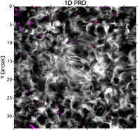
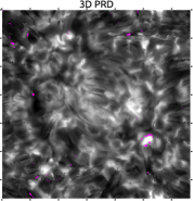
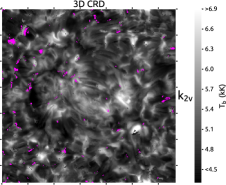
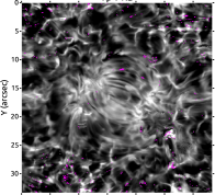
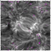
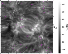
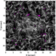
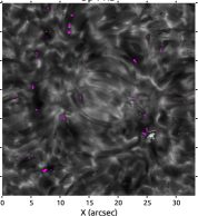
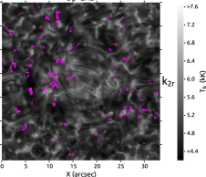
Figure 8: Images in the Mg II k line computed from the 3D Bifrost snapshot at $\mu_{\mathrm{Z}}=1$. Rows: blue emission peak k_2v (top), central depression k₃ (middle), and the red emission peak k_2r (bottom). Columns: computations in 1D PRD (left), 3D PRD (middle), and 3D CRD (right). The intensity is shown as a brightness temperature: $B_{\nu}(T_{\mathrm{b}})=I_{\nu}$. Fuchsia-colored spots indicate coordinates where a feature is not present or misidentified. The brightness scale for all images in a row is identical and indicated in the colorbar on the right side.

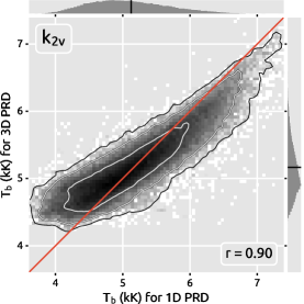
Figure 9: Joint probability density functions of the brightness temperature in Mg II k_2v (left), k₃ (center), and k_2r (right) computed in different cases. Horizontal axes are 1D PRD (left and right panels) and 3D CRD (center). Vertical axes are all 3D PRD. The color of the JPDFs displays the logarithm of the number of counts ranging from white (smallest) to black (biggest). The three nested iso-contours encompass regions with 68%, 95%, and 99% of all pixels. The red lines denote $x=y$. The small side plots show 1D histograms for the horizontal (top) or vertical (right) axes with mean values indicated by short black lines. The Pearson correlation coefficient $r$ is given in an inset in each panel.

Figure 8 shows images of the brightness temperature in k_2r, k₃, and k_3r for the 1D PRD, 3D PRD, and 3D CRD computations. These features are not always present and sometimes the automated fitting routine misidentifies them. These locations are indicated with fuchsia-colored pixels.

We see that the k₃ images computed in 3D CRD and 3D PRD (middle row of Fig. 8) indeed look similar. As was already shown by Leenaarts et al. (2013a), the 1D PRD image appears very different than the images computed in 3D.

For the emission peak images (top and bottom rows) we see substantial differences between the 1D PRD and 3D PRD computations. The 1D PRD images have substantially higher contrast, and bright structures have much sharper edges than in the 3D PRD computations. Interestingly there is also a significant structural similarity between 3D PRD and 3D CRD.

Figure 9 illustrates the same points by showing joint probability density functions (JPDFs) between brightness temperatures computed in 3D PRD and those computed in 1D PRD for the emission peaks and 3D CRD for the central depression. The k₃ brightness temperature in 3D PRD is typically slightly higher than predicted by the 3D CRD computation.

For k_2v and k_2r we see that the contrast for the 3D PRD computation is lower than for the 1D PRD case. The 1D PRD computations underestimate the brightness where $T_{\mathrm{b}}<5$ kK, and overestimate it where $T_{\mathrm{b}}>5$ kK.

5.3.2 Average line profiles and center-to-limb variation

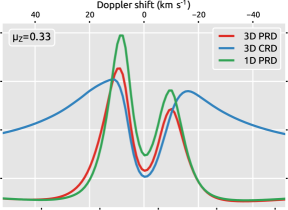
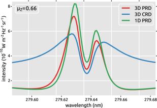
Figure 10: Mg II k line profiles for spatially-averaged intensity in 3D PRD (red), 3D CRD (blue), and 1D PRD (green) computed at different $\mu_{\mathrm{Z}}$ angles in the 3D Bifrost model atmosphere.

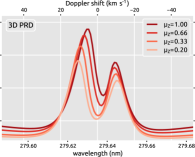
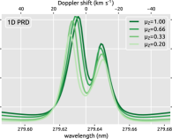
Figure 11: Same as in Fig. 10, but the line profiles, computed at different angles, are grouped separately for 3D CRD, 3D PRD, and 1D PRD.

Figures 10 and 11 display the center-to-limb variation of the spatially-averaged intensity profiles of the Mg II k line.

First, we discuss how PRD and 3D effects change the wavelength positions of the k_2v, k₃, and k_2r features. The 1D PRD approximation correctly predicts the wavelength positions of all the features, while the 3D CRD approximation does this only for the k₃ feature. Going towards the limb, we see similar blueshifts of the k₃ feature in 3D CRD, 1D PRD, and 3D PRD. We see the same effect in the k_2v peak in both PRD cases but a much stronger shift in 3D CRD. Going towards the limb, we see a slight redshift of the k_2r peak in both PRD cases and a strong redshift in 3D CRD. The peak separation $\lambda(\mathrm{k_{2r}})-\lambda(\mathrm{k_{2v}})$ slightly increases towards the limb in 3D PRD and it behaves similar in 1D PRD. However, in 3D CRD it strongly increases.

In short, one can use 1D PRD as a valid approximation for the wavelength positions of the k_2v and the k_2r emission peaks as well as for the k₃ absorption feature. The 3D CRD approximation is accurate only for the wavelength of the k₃ feature.

Second, we show how PRD and 3D effects change the intensities of the line profiles including the features.

As expected, the 3D CRD approximation is not valid for the intensities in the inner wings and in the emission peaks. It also underestimates the intensities of the line core at disk center, but this difference gets smaller towards the limb.

The 1D PRD approximation is very good for the inner wings, but it overestimates the intensities of all the features and this effect increases towards the limb.

We see asymmetries in the line profiles in all three cases.

In all three cases we see that the intensities of the k_2v peak is larger than the intensities of k_2r. This is caused by asymmetries in vertical velocity field in the simulation, for example by upward-propagating shocks (cf. Carlsson & Stein 1997, for a discussion of this effect in the Ca II H&K lines).

There is an interesting asymmetry in the flanks of the emission peaks in the 3D PRD case that is not present in the 1D PRD case (compare the red and green curves Fig. 10 between 279.60 nm and 279.63 nm). A similar asymmetry is present in 3D CRD, except that it happens further away from the line center because of the wider emission peaks. This asymmetry in the 3D computations must be caused by interaction between the velocity field in the simulation and the horizontal transport of radiation, and should be investigated in more detail.

In short, the intensities of the inner wings in the average line profile are well reproduced by the 1D PRD approximation. The line core is however not modeled accurately by 1D PRD. The 3D CRD approximation reproduces only the line core intensity towards the limb.

In summary, we have shown for the Mg II k line that its profile, as well as the profile features, are influenced by both PRD and 3D effects. The 1D PRD approximation reproduces the wavelength position of the features, and can be used to accurately compute intensities in the inner wings. The intensity and the wavelength position of k₃ can be computed using 3D CRD at disk center, but not towards the limb. Accurate quantitative modeling of the whole line profile and its center-to-limb variation requires 3D PRD.

6 Discussion and Conclusions

In this paper we presented an algorithm for 3D non-LTE radiative transfer including PRD effects in atmospheres with velocity fields. It improves on the algorithm described by Leenaarts et al. (2012b) by discretizing PRD line profiles on a frequency grid with intervals being integer multiples of a chosen fine resolution. Such a grid allows using fast linear interpolation with pre-computed indices and weights stored with a small memory footprint. This permits a relatively fast solution of the 3D non-LTE problem, costing 50 000–200 000 CPU hours to reach a converged solution in a model atmosphere with $252\times 252\times 496$ grid points.

We investigated the numerical properties of the algorithm in realistic use case scenario’s and found that it is stable, applicable to strongly scattering lines like Ly $\alpha$, and sufficiently fast to be practically useful for the computation of time-series of snapshots from radiation-MHD simulations.

We presented an application to the formation of the Mg II h&k lines in the solar chromosphere. We found that the conclusion of Leenaarts et al. (2013a) that the k_2v and k_2r emission peaks for disk-center intensities can be accurately modeled using 1D PRD computations to be incorrect. The emission peaks are affected by both PRD and 3D effects, and should be modeled using both 3D and PRD effects simultaneously.

We also showed that the center-to-limb variation in 1D PRD, 3D CRD, and 3D PRD is markedly different. The method presented in this paper will allow comparison of numerical models and observations of PRD-sensitive lines not only for disk-center observations but also for observations towards the limb.

We are planning to perform a detailed comparison of the center-to-limb variation of the Mg II h&k lines as predicted by numerical simulations to IRIS observations, such as those by Schmit et al. (2015).

Appendix A Algorithms for the forward and backward transforms

A.1 Definitions and notations

The notations adopted in this Appendix are as follows. Parentheses ( and ) denote functional dependence, e.g., $\rho(\@vec{n},q)$, while brackets [ and ] denote array indexing, e.g., $q[i]$. Both notations should not be mistaken with intervals of real numbers, e.g., $x\in{[x_{\mathrm{A}},x_{\mathrm{B}})}$ means $x_{\mathrm{A}}\leq x<x_{\mathrm{B}}$. A different notation is used for ordered ranges of integers, e.g., $l=m,\dotsc,n$. Index tuples, which subscript arrays, are always named explicitly not to confuse them with open intervals, e.g., index tuple $(x,y,z,\mu,i)$. Sections of 1D-arrays are denoted by their initial and terminal subscripts separated by a colon, e.g., $q[i_{\mathrm{red}}{:}i_{\mathrm{blue}}]$. Names of auxiliary arrays are given in typewriter font, e.g., $\mathtt{map}[i]$, while other quantities, stored in arrays, are given in roman font, e.g., $\@vec{\varv}[x,y,z]$. The symbol $\mapsto$ means interpolation, the symbol $\leftarrow$ is an assignment, and the symbol $\overset{+}{\leftarrow}$ indicates an increment.

As mentioned in Sect. 2.3, we deal with the inertial frame and the comoving frame. Frequency-dependent quantities from both frames are Doppler-shifted in frequency with respect to each other due to the velocity field $\@vec{\varv}[x,y,z]$ given in the model atmosphere. The forward transform converts the specific intensity $I$ from the inertial frame to the comoving frame by taking into account Doppler shifts of frequencies, while the backward transform does the same in the opposite direction for the profile ratio $\rho$. All quantities in the comoving frame are marked with a superscript ${\!}^{\star\!}$: specific intensity $I^{\star\!}$, angle-averaged intensity $J^{\star\!}$, profile ratio $\rho^{\star\!}$, and frequency $q^{\star\!}$. The same quantities in the inertial frame have no superscript. The only exception is for line frequencies, which always appear in indexed array form as either $q[i]$ or $q[j]$, where different subscripts are used to tell to which of the frames $q$ belongs. For brevity, we say ‘inertial/comoving $X$’ instead of ‘quantity $X$ in the inertial/comoving frame’.

Computations are performed in a Cartesian subdomain of $N_{\mathrm{X}}N_{\mathrm{Y}}N_{\mathrm{Z}}$ grid points with indices $x=x_{\mathrm{min}},\dotsc,x_{\mathrm{max}}$, $y=y_{\mathrm{min}},\dotsc,y_{\mathrm{max}}$, and $z=z_{\mathrm{min}},\dotsc,z_{\mathrm{max}}$. Angle-dependent quantities are represented on an angle quadrature with $N_{\mu}$ rays having directions $\@vec{n}[\mu]\colon\mu=1,\dotsc,N_{\mu}$. Frequency-dependent quantities are discretized on a grid of $N_{\nu}$ points having frequencies $q[i]\colon i=i_{\mathrm{red}},\dotsc,i_{\mathrm{blue}}$ (see Sect. A.1.1 for the definition of $q$). Subscript $i$ denotes frequency points in the inertial grid, while subscript $j$ denotes them in the comoving grid, such that their ranges and frequency grid values are identical: $i_{\mathrm{red}}=j_{\mathrm{red}}$, $i_{\mathrm{blue}}=j_{\mathrm{blue}}$, and $q[i]=q[j]$ if $i=j$. For the equidistant interpolation (see Sect. A.5), we use two extra grids with two different subscripts: $m$ for the fine inertial grid, and $n$ for the fine comoving grid.

We use three short-hands ‘knot’, ‘lie’, and ‘match’ with the following meanings. Following textbooks on interpolation methods, we refer to frequency grid points as knots, e.g., saying ‘comoving knot $i$’ we mean ‘frequency $q[i]$ in the comoving frame’. Saying ‘inertial knot $i$ lies on the comoving interval ${[j,j+1)}$’, we mean that the frequency $q[i]$ in the inertial frame is between two frequencies $q^{\star\!}[j]$ and $q^{\star\!}[j+1]$ in the comoving frame, i.e., $q^{\star\!}[j]\leq q[i]<q^{\star\!}[j+1]$. Saying ‘inertial knot $i$ matches the comoving knot $j$’, we mean that $q[i]=q^{\star\!}[j]$.

In the listings of algorithms, we implicitly use an advantage of the iteration loop control in Fortran do-statements to avoid if-statements: if the increment is positive/negative and the starting index is larger/smaller than the ending index, then no iterations are performed. The same applies to array sections: if the increment is positive/negative and the lower bound is larger/smaller than the upper bound, then no array elements are indexed. We also use the Fortran feature that array subscripts can start at any integer number.

A.1.1 Doppler transform

Usually, velocities in the upper atmosphere of the Sun do not exceed 150 km s^-1 so that $\beta\equiv\varv/c<5\cdot 10^{-4}$ and we can adopt a non-relativistic approximation for the Doppler transform in both directions neglecting $O(\beta^{2})$ terms:

$$\nu^{\star\!} =\nu\phantom{{}^{\star\!}}\Bigl{(}1-\dfrac{\@vec{n}\cdot\@vec{\varv}}{c}\Bigr{)},$$ (20)

$$\nu\phantom{{}^{\star\!}} =\nu^{\star\!}\Bigl{(}1+\dfrac{\@vec{n}\cdot\@vec{\varv}}{c}\Bigr{)}.$$ (21)

We also neglect aberration of light so that $\@vec{n}^{\star\!}=\@vec{n}$.

For convenience, we express frequency $\nu$ as dimensionless frequency displacement $q$ given in Doppler units $\Delta\nu_{\mathrm{D}}=\nu_{0}\varv_{\mathrm{B}}/c$:

$$q\equiv\dfrac{\nu-\nu_{0}}{\Delta\nu_{\mathrm{D}}}=\Bigl{(}\dfrac{\nu}{\nu_{0}}-1\Bigr{)}\dfrac{c}{\varv_{\mathrm{B}}},$$ (22)

with $\nu_{0}$ the line center frequency, and $\varv_{\mathrm{B}}$ the characteristic broadening velocity, which we typically set to a value of a few km s${}^{-1}\!$.

Using frequencies $q$, we can linearize the Doppler transform in Eqs. (20)–(21):

$$q^{\star\!} =q\phantom{{}^{\star\!}}-q_{\mu},$$ (23)

$$q\phantom{{}^{\star\!}} =q^{\star\!}+q_{\mu},$$ (24)

with the Doppler shift along direction $\@vec{n}[\mu]$ given by a scalar product

$$q_{\mu}=\dfrac{\@vec{n}[\mu]\cdot\@vec{\varv}[x,y,z]}{\varv_{\mathrm{B}}}.$$ (25)

The linear approximation in Eqs. (23)–(24) is valid if $|q|\,\varv_{\mathrm{B}}\ll c$, which is true even for the most extreme situation of the H I Ly $\alpha$ line.

A.1.2 Piecewise linear interpolation

Since we are restricted by available computing time, we employ the fastest and the easiest method: piecewise linear interpolation and constant extrapolation. We especially benefit from it when we use equidistant frequency grids.

Given data samples $y_{\mathrm{L}}$ and $y_{\mathrm{R}}$ on two knots L and R with frequencies $q_{\mathrm{L}}$ and $q_{\mathrm{R}}$, the interpolant value $y$ at frequency $q\in{[q_{\mathrm{L}},q_{\mathrm{R}})}$ is a linear combination of both samples

$$y=\varw\,y_{\mathrm{L}}+(1-\varw)\,y_{\mathrm{R}},$$ (26)

where knot L contributes with the left-hand-side (l.h.s.) weight

$$\varw=\frac{q_{\mathrm{R}}-q\phantom{{}_{\mathrm{R}}}}{q_{\mathrm{R}}-q_{\mathrm{L}}}$$ (27)

and knot R contributes with the right-hand-side (r.h.s.) weight

$$1-\varw=\frac{q\phantom{{}_{\mathrm{R}}}-q_{\mathrm{L}}}{q_{\mathrm{R}}-q_{\mathrm{L}}}.$$ (28)

An advantage of linear interpolation over other schemes is that only one weight $\varw$ has to be known, the other one always complements $\varw$ to one.

Constant extrapolation is used if $q$ is beyond the interpolation range ${[q_{\mathrm{A}},q_{\mathrm{Z}})}$ set by the outermost knots A and Z. If $q<q_{\mathrm{A}}$, then $y=y_{\mathrm{A}}$, and if $q_{\mathrm{Z}}\leq q$, then $y=y_{\mathrm{Z}}$.

When necessary, we call a standard function

$$Y\leftarrow\mathrm{interpolate}\big{(}X,\@vec{x},\@vec{y}\big{)},$$ (29)

which evaluates an interpolant $Y$ at a given coordinate $X$ for data values $\@vec{y}$ sampled on knots with coordinates $\@vec{x}$. It uses a correlated bisection search (Press et al. 1992, see p. 111):

$$l\leftarrow\mathrm{locate}\big{(}X,\@vec{x},l^{\prime}\big{)},$$ (30)

which returns the index $l$ of the array $\@vec{x}$ such that $\@vec{x}[l]\leq X<\@vec{x}[l+1]$. The input parameter $l^{\prime}$ is used to initialize the search.

A.1.3 Interval coverage

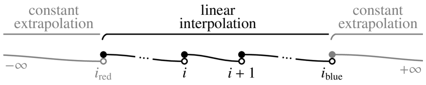
Figure 12: Adopted coverage of the interpolation intervals. Linear interpolation is performed on internal right-open intervals, given in black. Constant extrapolation is performed on outer semi-infinite intervals, given in gray. Lines are sloped to show their end points separately.

Given a monotonically ordered set of knots $\{i\colon i=i_{\mathrm{red}},\dotsc,i_{\mathrm{blue}}\}$ representing a line frequency grid $q[i]$ from the leftmost knot $i_{\mathrm{red}}$ to the rightmost knot $i_{\mathrm{blue}}$, we complement it by two infinite points ${-}\infty$ and ${+}\infty$ for convenience. We perform interpolation and extrapolation on right-open intervals to avoid using values at knots twice on adjacent intervals. That is to say, linear interpolation is carried out on ${[i,i+1)}\colon i=i_{\mathrm{red}},\dotsc,i_{\mathrm{blue}}-1$ intervals, and constant extrapolation is performed on the $({-}\infty,i_{\mathrm{red}})$ and ${[i_{\mathrm{blue}},{+}\infty)}$ intervals as shown in Fig. 12.

A.1.4 Forward transform

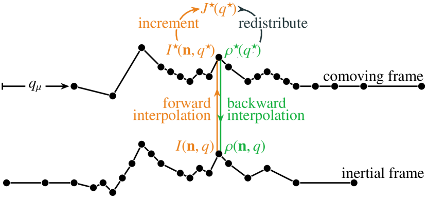
Figure 13: Doppler transform between two frequency grids: the inertial-frame grid $q$ (bottom) and the comoving-frame grid $q^{\star\!}$ (top). Both grids are identical, but the comoving one is displaced in increasing direction of frequency by Doppler shift $q_{\mu}$: $q^{\star\!}=q-q_{\mu}$. The forward transform (orange) consists of forward interpolation for the specific intensity $I\mapsto I^{\star\!}$ and an increment of the angle-averaged intensity $J^{\star\!}$. The backward transform (green) is backward interpolation for the profile ratio $\rho^{\star\!}\mapsto\rho$.

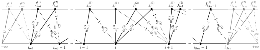
Figure 14: Illustration of the forward interpolation. Interpolation is performed for comoving knots $j$ (top line) on intervals between the inertial knots $i$ (bottom line). Each inertial interval ${[i,i+1)}$ contains zero or more comoving knots denoted by $j_{i}^{\,(\alpha)}\colon\alpha=1,\dotsc,\alpha_{\mathrm{max}}$. Corresponding l.h.s. weights $\varw_{i}^{(\alpha)}$ (solid) and r.h.s. weights $1-\varw_{i}^{(\alpha)}$ (dotted) are shown by sloped lines. Constant extrapolation is performed with $1-\varw_{{-}\infty}^{(\alpha)}=1$ weights on the $({-}\infty,i_{\mathrm{red}})$ interval, and with $\varw_{i_{\mathrm{blue}}}^{(\alpha)}=1$ weights on the ${[i_{\mathrm{blue}},{+}\infty)}$ interval, both drawn with gray color. Note that the comoving knot $j_{i}^{\,(1)}$, which exactly matches the inertial knot $i$, lies on the the ${[i,i+1)}$ interval, in agreement with the right-openness of all intervals.

After the formal solution of the transfer equation is done at coordinate $(x,y,z)$ for direction $\@vec{n}[\mu]$ at frequency $q[i]$, we have the inertial specific intensity $I\bigl{(}\@vec{n}[\mu],q[i]\bigr{)}=I[x,y,z,\mu,i]$. Owing to the local nature of the intensity redistribution and the Doppler transform, we drop dependencies on the spatial coordinates in the formulas given below.

The forward transform consists of two parts (see orange notations in Fig. 13). First, the inertial specific intensity $I\bigl{(}\@vec{n}[\mu],q[i]\bigr{)}$ is interpolated to get the comoving specific intensity $I^{\star\!}\bigl{(}\@vec{n}[\mu],q^{\star\!}\bigr{)}$ at comoving frequency $q^{\star\!}=q[i]-q_{\mu}$:

$$I\bigl{(}\@vec{n}[\mu],q[i]\bigr{)}\mapsto I^{\star\!}\bigl{(}\@vec{n}[\mu],q^{\star\!}\bigr{)},$$ (31)

This part is also called forward interpolation. Second, the interpolated intensity $I^{\star\!}\bigl{(}\@vec{n}[\mu],q^{\star\!}\bigr{)}$ contributes into (increments) the comoving angle-averaged intensity $J^{\star\!}\bigl{(}q^{\star\!}\bigr{)}$:

$$J^{\star\!}\bigl{(}q^{\star\!}\bigr{)}\overset{+}{\leftarrow}\dfrac{\omega_{\mu}}{4\pi}I^{\star\!}\bigl{(}\@vec{n}[\mu],q^{\star\!}\bigr{)},$$ (32)

with $\omega_{\mu}/4\pi$ the quadrature weight for direction $\@vec{n}[\mu]$. If we combine Eq. (31) with Eq. (32) for all $\mu$, we obtain the angle-discretized form of Eq. (16):

$$J^{\star\!}\bigl{(}q^{\star\!}\bigr{)}=\sum_{\mu=1}^{N_{\mu}}\dfrac{\omega_{\mu}}{4\pi}I\bigl{(}\@vec{n}[\mu],q^{\star\!}+q_{\mu}\bigr{)}.$$ (33)

This equation implies first a transform of the intensity from the inertial to the comoving frame, which numerically corresponds to an interpolation. The problem is that the intensity $I$ is not known for all frequencies simultaneously, due to the way how the formal solution is performed numerically in the Multi3D code. Instead, we compute Eqs. (31)–(32) incrementally from each $I\bigl{(}\@vec{n}[\mu],q[i]\bigr{)}$, without ever having the intensity for other inertial frequencies and angles in memory at the same time.

Forward interpolation $I\bigl{[}\mu,i\bigr{]}\mapsto I^{\star\!}\bigl{[}\mu,j\bigr{]}$ contributes the intensity $I$ at the inertial knot $i$ to intensities $I^{\star\!}$ at related comoving knots $j$. The related knots $j$ lie on the left and right neighboring intervals on both sides of $i$. We adopt the following notation for a series of the comoving knots lying on the inertial interval ${[i,i+1)}$: $j_{i}^{\,(\alpha)}$ denote the related knots, and $\varw_{i}^{(\alpha)}$ denote the corresponding l.h.s. interpolation weights, where the subscript $i$ is the starting index of the inertial interval and the counter $\alpha=1,\dotsc,\alpha_{\mathrm{max}}$ numbers all the knots in the series. There are zero or more $(\alpha_{\mathrm{max}}\geq 1)$ comoving knots, whose indices $j_{i}^{\,(\alpha)}$ and weights $\varw_{i}^{(\alpha)}$ depend on the positions and relative distances between their comoving frequencies $q^{\star\!}=q[j]+q_{\mu}$ and the inertial frequency $q[i]$.

This is illustrated in Fig. 14. The knot $i$ always has two neighbors $i-1$ and $i+1$ so that related knots $j$ are interpolated on the left ${[i-1,i)}$ and right ${[i,i+1)}$ intervals. The inertial intensity $I$ at the knot $i$ is interpolated to the comoving intensity $I^{\star}$ at knots $j_{i-1}^{\,(\alpha)}$ using r.h.s. weights $1-\varw_{i-1}^{(\alpha)}$ on the left interval, and at knots $j_{i}^{\,(\alpha)}$ using l.h.s. weights $\varw_{i}^{(\alpha)}$ on the right interval. At the ends of the frequency grid, weights on the infinite intervals are always equal to unity to force constant extrapolation: $1-\varw_{i-1}^{(\alpha)}=1-\varw_{{-}\infty}^{(\alpha)}=1$ for $i=i_{\mathrm{red}}$, and $\varw_{i}^{(\alpha)}=\varw_{i_{\mathrm{blue}}}^{(\alpha)}=1$ for $i=i_{\mathrm{blue}}$.

Plugging expressions for $j$ and $\varw$ into the discretized Eqs. (31)–(32) we get

$$J^{\star\!}\bigl{[}j_{i-1}^{\,(\alpha)}\bigr{]} \overset{+}{\leftarrow}\Bigl{(}1-\varw_{i-1}^{(\alpha)}\Bigr{)}\dfrac{\omega_{\mu}}{4\pi}I\bigl{[}\mu,i-1\bigr{]} \quad\text{on }{[i-1,i)},$$ (34)

$$J^{\star\!}\bigl{[}j_{i}^{\,(\alpha)}\bigr{]} \overset{+}{\leftarrow}\mspace{43.0mu}\varw_{i}^{(\alpha)}\dfrac{\omega_{\mu}}{4\pi}I\bigl{[}\mu,i\bigr{]} \quad\text{on }{[i,i+1)}.$$ (35)

A.1.5 Backward transform

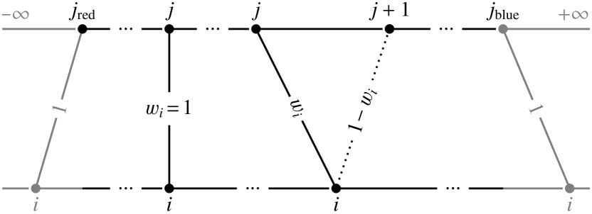
Figure 15: Illustration of the backward interpolation. Interpolation is performed for inertial knots $i$ (bottom line) on intervals between comoving knots $j$ (top line). Interpolation weights are indicated on sloped lines connecting corresponding knots between the frames. Linear interpolation is used for internal inertial knots $i$ that lie on the internal comoving intervals ${[j,j+1)}$ with l.h.s. $\varw_{i}$ (solid) and r.h.s. $1-\varw_{i}$ (dotted) weights. Weights are named with respect to the comoving frame so that the line slopes are opposite to those in the forward interpolation. Constant extrapolation with unity weights is used for inertial knots $i$ exactly matching comoving knots $j$, or for inertial knots that lie on the ${({-}\infty,j_{\mathrm{red}})}$ or ${[j_{\mathrm{blue}},{+}\infty)}$ intervals. Both end cases are given in gray color.

Once $J^{\star}$ has been fully accumulated, we compute the comoving profile ratio $\rho^{\star\!}\bigl{(}q[j]\bigr{)}=\rho^{\star\!}[x,y,z,j]$ and keep it in memory for all frequency knots $j=j_{\mathrm{red}},\dotsc,j_{\mathrm{blue}}$ simultaneously. This makes the backward transform much easier than the forward one, because we can employ a standard interpolation.

The backward transform can be directly evaluated because it is just an interpolation from the comoving frame to the inertial frame (see green notations in Fig. 13):

$$\rho^{\star\!}\bigl{(}q[i]-q_{\mu}\bigr{)}\mapsto\rho\bigl{(}\@vec{n}[\mu],q[i]\bigr{)}.$$ (36)

As follows from Fig. 15, each $\rho\bigl{(}\@vec{n}[\mu],q[i]\bigr{)}$ depends on either one or two comoving knots $j$.

It depends on two knots, if the inertial knot $i$ lies on the comoving interval ${[j,j+1)}$, where both $j$ and $j+1$ are internal knots ($j_{\mathrm{red}}\leq j<j+1\leq j_{\mathrm{blue}}$), i.e., $q[j]+q_{\mu}\leq q[i]<q[j+1]+q_{\mu}$. In this case we do linear interpolation:

$$\rho[\mu,i]=\varw_{i}\,\rho^{\star\!}[j]+(1-\varw_{i})\,\rho^{\star\!}[j+1].$$ (37)

For the backward transform, knots and weights are always denoted by $j$ and $\varw_{i}$ with no superscript $(\alpha)$ to tell them from knots $j_{i}^{\,(\alpha)}$ and weights $\varw_{i}^{(\alpha)}$ for the forward transform.

It depends on one knot, if the inertial knot $i$ matches the comoving knot $j$, i.e., $q[i]=q[j]+q_{\mu}$. It also depends on one knot, if the inertial knot $i$ lies on intervals before $j_{\mathrm{red}}$ or after $j_{\mathrm{blue}}$, which means $q[i]<q[j_{\mathrm{red}}]+q_{\mu}$ or $q[j_{\mathrm{blue}}]+q_{\mu}\leq q[i]$, because we use constant extrapolation. Therefore, in those three cases:

$$\rho[\mu,i] =\rho^{\star\!}[j],$$ or (38)

$$\rho[\mu,i] =\rho^{\star\!}[j_{\mathrm{red}}],$$ or (39)

$$\rho[\mu,i] =\rho^{\star\!}[j_{\mathrm{blue}}].$$ (40)

A.2 General interpolation

One can perform the searches and interpolations described in Sects. A.1.4–A.1.5 on the fly. This does not require any additional storage, and can be used for a frequency grid of arbitrary spacing, but the algorithm is slow. We call this algorithm general interpolation.

A.2.1 General forward transform

Data: Specific intensity $I[x,y,z,\mu,i]$ at frequency $q[i]$ and direction $\@vec{n}[\mu]$ in the inertial frame.

Result: Incremented angle-averaged intensity $J^{\star\!}[x,y,z,j]$ at corresponding frequencies $q[j]$ in the comoving frame.

$q_{\mu}\leftarrow\bigl{(}\@vec{n}[\mu]\cdot\@vec{\varv}[x,y,z]\bigr{)}/\varv_{\mathrm{B}}$

$q^{\star}_{\mathrm{L}}\leftarrow q\mathmakebox[\widthof{${\bigl{[}\min(i+1,i_{\mathrm{blue}})\bigr{]}}$}][l]{\bigl{[}\max(i-1,i_{\mathrm{red}})\bigr{]}}-q_{\mu}$

$q^{\star}_{\mathrm{C}}\leftarrow q\mathmakebox[\widthof{${\bigl{[}\min(i+1,i_{\mathrm{blue}})\bigr{]}}$}][l]{\bigl{[}i\bigr{]}}-q_{\mu}$

$q^{\star}_{\mathrm{R}}\leftarrow q\bigl{[}\min(i_{\mathrm{blue}},i+1)\bigr{]}-q_{\mu}$

if $q^{\star}_{\mathrm{L}}\neq q^{\star}_{\mathrm{C}}$ then // Linear interpolation on $\bigl{(}q^{\star}_{\mathrm{L}},q^{\star}_{\mathrm{C}}\bigr{)}$:

      $\Delta\leftarrow q^{\star}_{\mathrm{C}}-q^{\star}_{\mathrm{L}}$

      for $j\leftarrow j_{\mathrm{red}}$ to $j_{\mathrm{blue}}$ do

           if $q^{\star}_{\mathrm{L}}<q[j]<q^{\star}_{\mathrm{C}}$ then

                $\xi^{\prime}\leftarrow\big{(}q[j]-q^{\star}_{\mathrm{L}}\big{)}/\Delta$

                 // The r.h.s. weight $1-\varw_{i-1}$.

                $J^{\star\!}[x,y,z,j]\overset{+}{\leftarrow}\xi^{\prime}\dfrac{\omega_{\mu}}{4\pi}I[x,y,z,\mu,i]$

               

          

     

else $q^{\star}_{\mathrm{L}}=q^{\star}_{\mathrm{C}}$ // Constant extrapolation on $\bigl{(}{-}\infty,q^{\star}_{\mathrm{C}}\bigr{)}$:

      for $j\leftarrow j_{\mathrm{red}}$ to $j_{\mathrm{blue}}$ do

           if $q[j]<q^{\star}_{\mathrm{C}}$ then

                $J^{\star\!}[x,y,z,j]\overset{+}{\leftarrow}\dfrac{\omega_{\mu}}{4\pi}I[x,y,z,i]$

               

          

     

if $q^{\star}_{\mathrm{C}}\neq q^{\star}_{\mathrm{R}}$ then // Linear interpolation on ${\bigl{[}q^{\star}_{\mathrm{C}},q^{\star}_{\mathrm{R}}\bigr{)}}$:

      $\Delta\leftarrow q^{\star}_{\mathrm{R}}-q^{\star}_{\mathrm{C}}$

      for $j\leftarrow j_{\mathrm{red}}$ to $j_{\mathrm{blue}}$ do

           if $q^{\star}_{\mathrm{C}}\leq q[j]<q^{\star}_{\mathrm{R}}$ then

                $\xi\leftarrow\big{(}q^{\star}_{\mathrm{R}}-q[j]\big{)}/\Delta$

                 // The l.h.s. weight $\varw_{i}$.

                $J^{\star\!}[x,y,z,j]\overset{+}{\leftarrow}\xi\dfrac{\omega_{\mu}}{4\pi}I[x,y,z,i]$

               

          

     

else $q^{\star}_{\mathrm{C}}=q^{\star}_{\mathrm{R}}$ // Constant extrapolation on ${\bigl{[}q^{\star}_{\mathrm{C}},{+}\infty\bigr{)}}$:

      for $j\leftarrow j_{\mathrm{red}}$ to $j_{\mathrm{blue}}$ do

           if $q^{\star}_{\mathrm{C}}\leq q[j]$ then

                $J^{\star\!}[x,y,z,j]\overset{+}{\leftarrow}\dfrac{\omega_{\mu}}{4\pi}I[x,y,z,i]$

               

          

     

Alg. 1 General forward transform. Comments in this algorithm and those listed below are given in slanted text after ‘//’.

We search for all comoving knots $j$ that lie on the intervals ${[i-1,i)}$ and ${[i,i+1)}$, i.e., whose comoving frequencies $q^{\star\!}=q[j]+q_{\mu}$ are either between $q[i-1]$ and $q[i]$, or between $q[i]$ and $q[i+1]$.

We take the current inertial knot $i$ and its left neighbor $\max(i-1,i_{\mathrm{red}})$ and right neighbor $\min(i_{\mathrm{blue}},i+1)$. We use $\max()$ and $\min()$ to keep the neighbors within the frequency grid range $i=i_{\mathrm{red}},\dotsc,i_{\mathrm{blue}}$. For these knots we compute their frequencies in the comoving frame, which we denote by

$$q^{\star}_{\mathrm{L}} =q\bigl{[}\max(i-1,i_{\mathrm{red}})\bigr{]} -q_{\mu},$$ (41)

$$q^{\star}_{\mathrm{C}} =q\bigl{[}i\bigr{]} -q_{\mu},$$ (42)

$$q^{\star}_{\mathrm{R}} =q\bigl{[}\min(i_{\mathrm{blue}},i+1)\bigr{]} -q_{\mu}.$$ (43)

Therefore, the comoving knots $j$ related to the inertial knot $i$ are those, whose frequencies $q[j]$ belong to the ${\bigl{[}q^{\star}_{\mathrm{L}},q^{\star}_{\mathrm{C}}\bigr{)}}$ or ${\bigl{[}q^{\star}_{\mathrm{C}},q^{\star}_{\mathrm{R}}\bigr{)}}$ intervals.

The knots $j$ lie either on the left or on the right side of $q^{\star}_{\mathrm{C}}$, and they might fall outside the frequency coverage of the line. We thus have four different cases to test for and apply Eqs. (34)–(35). Algorithm 1 shows the forward transform in detail.

A.2.2 General backward transform

Data: Profile ratio $\rho^{\star\!}[x,y,z,j]$ for all frequencies $q[j]\colon j=j_{\mathrm{red}},\dotsc,j_{\mathrm{blue}}$ in the comoving frame.

Result: Profile ratio $\rho[x,y,z,\mu,i]$ for given frequency $q[i]$ and direction $\@vec{n}[\mu]$ in the inertial frame.

$q_{\mu}\leftarrow\big{(}\@vec{n}[\mu]\cdot\@vec{\varv}[x,y,z]\big{)}/\varv_{\mathrm{B}}$

$\rho[x,y,z,\mu,i]\leftarrow\mathrm{interpolate}\big{(}\,X=q[i]-q_{\mu},$

                                 $\@vec{x}=q[j_{\mathrm{red}}{:}j_{\mathrm{blue}}],$

                                 $\@vec{y}=\rho^{\star\!}[x,y,z,j_{\mathrm{red}}{:}j_{\mathrm{blue}}]\,\big{)}$

Alg. 2 General backward transform.

Algorithm 2 gives the backward transform, which is just an interpolation. It is performed by using Eq. (29) with $Y=\rho[x,y,z,\mu,i]$, $X=q[i]-q_{\mu}$, $\@vec{x}=q[j_{\mathrm{red}}{:}j_{\mathrm{blue}}]$, and $\@vec{y}=\rho^{\star\!}[x,y,z,j_{\mathrm{red}}{:}j_{\mathrm{blue}}]$.

A.3 Precomputed interpolation

The general algorithm given in Sect. A.2 is slow because for each $x$, $y$, $z$, $\mu$, and $i$ we perform two linear searches in the forward transform and a correlated bisection search in the backward transform along the full frequency range $j=j_{\mathrm{red}},\dotsc,j_{\mathrm{blue}}$.

To speed up the computations, one can precompute and store for each index tuple $(x,y,z,\mu,i)$ the comoving knots $j_{i}^{\,(\alpha)}$ and the l.h.s weights $\varw_{i}^{(\alpha)}$ used in the forward transform and the nearest comoving knot $j_{i}$ and its l.h.s. weight $\varw_{i}$ used in the backward transform.

A.3.1 Precomputation for the forward interpolation

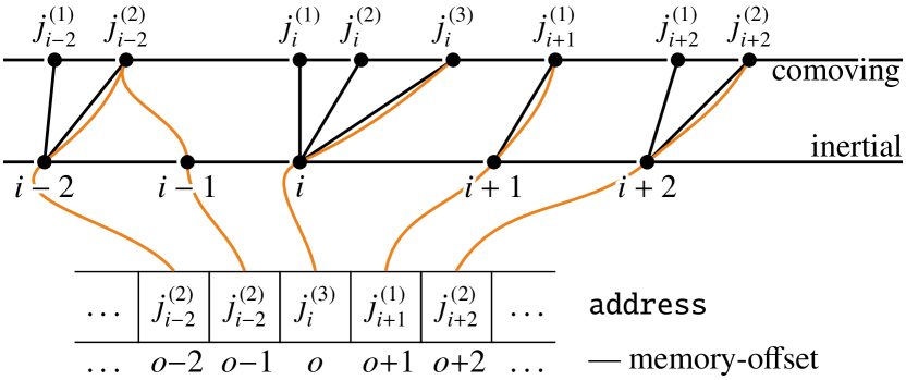
Figure 16: Illustrative contents of the address array for the forward precomputed interpolation. In the inertial frame (bottom black line), knots have indices $i$. In the comoving frame (top black line), knots that lie on the inertial interval ${[i,i+1)}$, have indices $j_{i}^{\,(\alpha)}\colon\alpha=1,\dotsc,\alpha_{\mathrm{max}}$ if at least one such knot exists. For each $i$, corresponding memory-offset $o$ is computed such that $\mathtt{address}[o]$ points to $j_{i}^{\,(\alpha_{\mathrm{max}})}$. Orange lines indicate $i{\to}\mathtt{address}[o]{\to}j_{i}^{\,(\alpha_{\mathrm{max}})}$ correspondence. Solid black lines connecting $i$ to $j_{i}^{\,(\alpha)}$, indicate l.h.s. weights $\varw_{i}^{(\alpha)}$. There is no contribution from knot $i-1$, because interval ${[i-1,i)}$ does not contain any comoving knots. In this case, $\mathtt{address}[o-1]$ points to the knot $j_{i-2}^{\,(2)}$ that lies on the previous interval. Note, that address keeps addresses but not the values of the shown comoving knots, those are stored in forward_j instead.

Data: Line frequencies $q[i_{\mathrm{red}}{:}i_{\mathrm{blue}}]$, directions $\@vec{n}[1{:}N_{\mu}]$, velocities $\@vec{\varv}[x_{\mathrm{min}}{:}x_{\mathrm{max}},y_{\mathrm{min}}{:}y_{\mathrm{max}},z_{\mathrm{min}}{:}z_{\mathrm{max}}]$.

Result: Arrays address, forward_j, and forward_w.

$\mathtt{address}[]\leftarrow 0$

  // Initialize array address

$c\leftarrow 0$

  // and its counter.

for $x\leftarrow x_{\mathrm{min}}$ to $x_{\mathrm{max}}$ do

      for $y\leftarrow y_{\mathrm{min}}$ to $y_{\mathrm{max}}$ do

           for $z\leftarrow z_{\mathrm{min}}$ to $z_{\mathrm{max}}$ do

                for $\mu\leftarrow 1$ to $N_{\mu}$ do

                     $q_{\mu}\leftarrow\big{(}\@vec{n}[\mu]\cdot\@vec{\varv}[x,y,z]\big{)}/\varv_{\mathrm{B}}$

                     $i\leftarrow i_{\mathrm{red}}-1$

                      // Start searching from the leftmost

                    

                      // knot $({-}\infty)$ in the inertial frame.

                     for $j\leftarrow j_{\mathrm{red}}$ to $j_{\mathrm{blue}}$ do // For each comoving knot $j$,

                         

                           // find which inertial knot $i$

                         

                           // contributes into it.

                          $q\leftarrow q[j]+q_{\mu}$

                           // Inertial frequency.

                          $i\leftarrow\mathrm{locate}\big{(}q,q[i_{\mathrm{red}}{:}i_{\mathrm{blue}}],i\big{)}$

                           // $q[i]\leq q<q[i+1]$

                          if $i_{\mathrm{red}}\leq i<i_{\mathrm{blue}}$ then // Linear interpolation

                               $\varw\leftarrow\dfrac{q[i+1]-q\mspace{16.0mu}}{q[i+1]-q[i]}$

                                // on ${[i,i+1)}$.

                              

                          else if $i=i_{\mathrm{red}}-1$ then // Constant extrapolation

                               $\varw\leftarrow 0$

                                // on ${({-}\infty,i_{\mathrm{red}})}$.

                              

                          else $i=i_{\mathrm{blue}}$ // Constant extrapolation

                               $\varw\leftarrow 1$

                                // on ${[i_{\mathrm{blue}},{+}\infty)}$.

                              

                         $o\leftarrow o(x,y,z,\mu,i)$

                           // Memory-offset by Eq. (A.3.1).

                         

                           // Fill address between $c$ and $o$

                         

                           // with the last stored address:

                          $\mathtt{address}[c+1{:}o-1]\leftarrow\mathtt{address}[c]$

                         

                         

                           // Update the current address:

                          $\mathtt{address}[o]\leftarrow\mathtt{address}[c]+1$

                          $c\leftarrow o$

                           // Set counter to the current address.

                          $\mathtt{forward\_j}\left[\mathtt{address}[c]\right]\leftarrow j$

                           // Save comoving

                          $\mathtt{forward\_w}\left[\mathtt{address}[c]\right]\leftarrow\varw$

                           // index & weight.

                         

                    

               

          

     

Alg. 3 Initialization of the precomputed forward interpolation.

In the forward transform, each inertial knot $i$ contributes to zero, one or more comoving knots $j$. Since the indices and the weights depend on $x$, $y$, $z$, $\mu$, $i$, and $\alpha$, they require jagged 6D-arrays with the last variable-length dimension for index $\alpha$. Neither Fortran nor C allows such a data structure in their latest language standards. A typical solution is to use 5D-arrays of pointers or linked lists. Both solutions are inconvenient and memory-inefficient because they require at least one 8-byte pointer (on the default 64-bit architecture) for each $\alpha$-series of $j_{i}^{\,(\alpha)}$ and $\varw_{i}^{(\alpha)}$.

It is more efficient to flatten these jagged arrays into two continous 1D-arrays, one for $j_{i}^{\,(\alpha)}$ (forward_j) and one for $\varw_{i}^{\,(\alpha)}$ (forward_w), which use the same indexing subscripts. Each of them consecutively stores $N_{\mathrm{X}}N_{\mathrm{Y}}N_{\mathrm{Z}}N_{\mu}N_{\nu}$ values.

In that case, for each index tuple $(x,y,z,\mu,i)$ we need to keep track of the related knots $j_{i}^{\,(\alpha)}$ and weights $\varw_{i}^{(\alpha)}$. We use the 1D-array address to do so.

For each $i=i_{\mathrm{red}}-1,\dots,i_{\mathrm{blue}}$, this array keeps the address of the last comoving knot $j_{i}^{\,(\alpha_{\mathrm{max}})}$ that lies on the inertial interval ${[i,i+1)}$. The extra knot $i_{\mathrm{red}}-1$ corresponds to the comoving frequency ${-}\infty$ and is needed to treat extrapolation beyond the left end of the frequency grid. For convenience, one more element is added to the address array at the beginning so that the array subscript $o$ starts from $-1$. Hence, address has $N_{\mathrm{X}}N_{\mathrm{Y}}N_{\mathrm{Z}}N_{\mu}(N_{\nu}+1)+1$ elements. The values stored in address start from 0 and are non-decreasing.

For each $x$, $y$, $z$, and $\mu$, we scan comoving knots $j=j_{\mathrm{red}},\dotsc,j_{\mathrm{blue}}$ to find the inertial nearest-left neighbor knot $i$ such that $q[i]\leq q[j]+q_{\mu}<q[i+1]$. Then we compute the l.h.s. weight $\varw$, using interpolation for internal knots, and constant extrapolation for external knots.

We set the subscript $o$ to the memory-offset given by the index tuple $(x,y,z,\mu,i)$:

$$o(x,y,z,\mu,i) =i-(i_{\mathrm{red}}-1)+(N_{\nu}+1)\cdot{}$$

$$\qquad(\mu-1+N_{\mu}\cdot{}$$

$$\qquad\quad(z-z_{\mathrm{min}}+N_{\mathrm{Z}}\cdot{}$$

$$\qquad\qquad(y-y_{\mathrm{min}}+N_{\mathrm{Y}}\cdot{}$$

$$\qquad\qquad\quad(x-x_{\mathrm{min}}))))).$$ (44)

It is important that the order of indices in the tuple follows the order of the nested for-loops in Algs. 3–4 so that address is filled continuously. Frequency is the fastest (continuous) dimension in memory.

At this point, counter $c$ subscripts the last modified element of address such that address[$c$] points to the last comoving knot saved in forward_j. Then we point address[$o$] to the current comoving knot $j$: since $j$ is stored contiguously in index_j, we use an incremented address of the last comoving knot:

$$\mathtt{address}[o]=\mathtt{address}[c]+1.$$ (45)

If $o=c$, then both the last and the current comoving knots lie on the same interval ${[i,i+1)}$ and address[$o=c$] is just incremented. If $o>c+1$, then there are inertial knots between the last and the current comoving knots, which do not contribute to any comoving knots. In this case, the elements of address between $c$ and $o$ are filled with address[$c$]:

$$\mathtt{address}[c+1{:}o-1]=\mathtt{address}[c],$$ (46)

so that they point to the last comoving knot. Then we adjust the counter $c$ to the current memory-offset $o$

$$c=o$$ (47)

and store the current comoving knot and its weight:

$$\mathtt{forward\_j}[\mathtt{address}[c]] =j,$$ (48)

$$\mathtt{forward\_w}[\mathtt{address}[c]] =\varw.$$ (49)

Now we proceed to the next comoving knot. We summarize this complicated procedure in Alg. 3 and illustrate it in Fig. 16.

A.3.2 Precomputation for the backward interpolation

Data: Line frequencies $q[i_{\mathrm{red}}{:}i_{\mathrm{blue}}]$, directions $\@vec{n}[1{:}N_{\mu}]$, velocities $\@vec{\varv}[x_{\mathrm{min}}{:}x_{\mathrm{max}},y_{\mathrm{min}}{:}y_{\mathrm{max}},z_{\mathrm{min}}{:}z_{\mathrm{max}}]$.

Result: Arrays backward_j and backward_w.

for $x\leftarrow x_{\mathrm{min}}$ to $x_{\mathrm{max}}$ do

      for $y\leftarrow y_{\mathrm{min}}$ to $y_{\mathrm{max}}$ do

           for $z\leftarrow z_{\mathrm{min}}$ to $z_{\mathrm{max}}$ do

                for $\mu\leftarrow 1$ to $N_{\mu}$ do

                     $q_{\mu}\leftarrow\big{(}\@vec{n}[\mu]\cdot\@vec{\varv}[x,y,z]\big{)}/\varv_{\mathrm{B}}$

                     $j\leftarrow j_{\mathrm{red}}-1$

                      // Start searching from the leftmost

                    

                      // knot $({-}\infty)$ in the comoving frame.

                     for $i\leftarrow i_{\mathrm{red}}$ to $i_{\mathrm{blue}}$ do // For each inertial knot $i$, find

                         

                           // which comoving knot $j$

                         

                           // contributes into it.

                          $q^{\star\!}\leftarrow q[i]-q_{\mu}$

                           // Comoving frequency.

                          $j\leftarrow\mathrm{locate}\big{(}q^{\star\!},q[j_{\mathrm{red}}{:}j_{\mathrm{blue}}],j\big{)}$

                           // $q[j]\,{\leq}\,q^{\star}{<}\,q[j{+}1]$

                          if $j=j_{\mathrm{red}}-1$ then

                               $\mathmakebox[\widthof{$\varw$}][l]{j^{\prime}}\leftarrow j_{\mathrm{red}}$

                                // Constant extrapolation

                               $\varw\leftarrow 1$

                                // on ${({-}\infty,j_{\mathrm{red}})}$.

                              

                          else if $j=j_{\mathrm{blue}}$ then

                               $\mathmakebox[\widthof{$\varw$}][l]{j^{\prime}}\leftarrow j_{\mathrm{blue}}$

                                // Constant extrapolation

                               $\varw\leftarrow 1$

                                // on ${[j_{\mathrm{blue}},{+}\infty)}$.

                              

                          else if $q^{\star}=q[j]$ then

                               $\mathmakebox[\widthof{$\varw$}][l]{j^{\prime}}\leftarrow j$

                                // Exact match of $j$ to $i$.

                               $\varw\leftarrow 1$

                              

                          else $j_{\mathrm{red}}\leq j<j_{\mathrm{blue}}$

                               $\mathmakebox[\widthof{$\varw$}][l]{j^{\prime}}\leftarrow j$

                                // Linear interpolation

                               $\varw\leftarrow\dfrac{q[j+1]-q^{\star}\;\>}{q[j+1]-q[j]}$

                                // on ${[j,j+1)}$.

                              

                         $\mathtt{backward\_j}[x,y,z,\mu,i]\leftarrow j^{\prime}$

                          // Store comoving

                          $\mathtt{backward\_w}[x,y,z,\mu,i]\leftarrow\varw$

                          // index and weight.

                         

                    

               

          

     

Alg. 4 Initialization of the precomputed backward interpolation.

Precomputation for the backward transform is similar to the one for the forward interpolation and is explained in Alg. 4, but there are two differences. First, each inertial knot $i$ has only one related comoving knot $j$, as illustrated in Fig. 15. This strict correspondence allows us to use 5D-arrays to store the indices and weights, no address array is needed. Second, we scan the inertial knots to find the related comoving knots, instead of the other way around.

A.3.3 Precomputed forward transform

Data: Specific intensity $I[x,y,z,\mu,i]$ at frequency $q[i]$ and direction $\@vec{n}[\mu]$ in the inertial frame.

Result: Incremented angle-averaged intensity $J^{\star\!}[x,y,z,j]$ at corresponding frequencies $q[j]$ in the comoving frame.

$o\leftarrow o(x,y,z,\mu,i)$

  // Memory-offset by Eq. (A.3.1)

$\mathmakebox[\widthof{$a_{i-2}$}][l]{a_{i}}\leftarrow\mathtt{address}[\mspace{14.0mu}o\mspace{15.0mu}]$

  // Addresses of comoving knots

$\mathmakebox[\widthof{$a_{i-2}$}][l]{a_{i-1}}\leftarrow\mathtt{address}[o-1]$

  // for current $i$, previous $i-1$, and

$\mathmakebox[\widthof{$a_{i-2}$}][l]{a_{i-2}}\leftarrow\mathtt{address}[o-2]$

  // pre-previous $i-2$ inertial knots.

for $a\leftarrow a_{i-2}+1$ to $a_{i-1}$ do // Interpolate on ${[i-1,i)}$:

      $\mathmakebox[\widthof{$\varw$}][l]{j}\leftarrow\mathtt{forward\_j}[a]$

      $\varw\leftarrow\mathtt{forward\_w}[a]$

      $J^{\star\!}[x,y,z,j]\overset{+}{\leftarrow}(1-\varw)\dfrac{\omega_{\mu}}{4\pi}I[x,y,z,\mu,i]$

       // Use r.h.s. weights.

     

for $a\leftarrow a_{i-1}+1$ to $a_{i}$ do // Interpolate on ${[i,i+1)}$:

      $\mathmakebox[\widthof{$\varw$}][l]{j}\leftarrow\mathtt{forward\_j}[a]$

      $\varw\leftarrow\mathtt{forward\_w}[a]$

      $J^{\star\!}[x,y,z,j]\overset{+}{\leftarrow}\varw\dfrac{\omega_{\mu}}{4\pi}I[x,y,z,\mu,i]$

       // Use l.h.s. weights.

     

Alg. 5 Precomputed forward transform.

With precomputed indices and weights, the forward transform can be done very quickly following Alg. 5. At grid point $(x,y,z)$, angle direction $\@vec{n}[\mu]$, and inertial frequency $q[i]$, we compute the memory-offset $o$ by using Eq. (A.3.1).

Now $a_{i}=\mathtt{address}[o]$ is the address of the last comoving knot $j_{i}^{\,(\max\alpha)}$ that lies on the inertial interval ${[i,i+1)}$. The previous knot $i-1$ has memory-offset $o-1$ so that $a_{i-1}=\mathtt{address}[o-1]$ is the address of the last comoving knot $j_{i-1}^{\,(\max\alpha)}$ that lies on the inertial interval ${[i-1,i)}$.

If $a_{i-1}<a_{i}$ then $a_{i}-a_{i-1}$ comoving knots lie on the interval ${[i,i+1)}$, and their addresses are $a_{i-1}+1,\dotsc,a_{i}$. Using these addresses, we extract indices the $j_{i}^{\,(\alpha)}$ from $\mathtt{forward\_j}$ and the l.h.s. weights $\varw_{i}^{(\alpha)}$ from $\mathtt{forward\_w}$ and perform the transform by using Eq. (35).

If $a_{i-1}=a_{i}$, then there are no comoving knots that lie on the inertial interval ${[i,i+1)}$ and no interpolation is done.

Applying the same procedure to the previous $i-1$ and pre-previous $i-2$ knots, we obtain the corresponding comoving indices $j_{i-1}^{\,(\alpha)}$ and r.h.s. weights $1-\varw_{i-1}^{(\alpha)}$ for the inertial interval ${[i-1,i)}$ and perform the transform by using Eq. (34).

It is necessary to use three knots (the current $i$, the previous $i-1$, and the pre-previous $i-2$) to compute the related indices and weights for both the ${[i-1,i)}$ and ${[i,i+1)}$ intervals because we store only the l.h.s. weights to save memory. This is why the subscript of address starts at $-1$, so that the algorithm handles the case $i=i_{\mathrm{red}}$ without using an if-statement.

A.3.4 Precomputed backward transform

Data: Profile ratio $\rho^{\star\!}[x,y,z,j]$ for all frequencies $q[j]\colon j=j_{\mathrm{red}},\dotsc,j_{\mathrm{blue}}$ in the comoving frame.

Result: Profile ratio $\rho[x,y,z,\mu,i]$ at given frequency $q[i]$ and direction $\@vec{n}[\mu]$ in the inertial frame.

$\mathmakebox[\widthof{$\varw$}][l]{j}\leftarrow\mathtt{backward\_j}[x,y,z,\mu,i]$

  // Comoving index

$\varw\leftarrow\mathtt{backward\_w}[x,y,z,\mu,i]$

  // and weight.

if $0\leq\varw<1$ then // Linear interpolation on ${[j,j+1)}$:

      $\rho[x,y,z,\mu,i]\leftarrow\varw\,\rho^{\star\!}[x,y,z,j]+\left(1-\varw\right)\rho^{\star\!}[x,y,z,j+1]$

     

else $\varw=1$ // Either constant extrapolation if $j\notin{[j_{\mathrm{red}},j_{\mathrm{blue}})}$,

      $\rho[x,y,z,\mu,i]\leftarrow\rho^{\star\!}[x,y,z,\mu,j]$

       // or $j$ exactly matches $i$.

     

Alg. 6 Precomputed backward transform.

With precomputed indices and weights the backward interpolation is performed as in Alg. 6. We select the proper type of interpolation from Eqs. (37)–(40) depending on the value of the r.h.s. weight $\varw$.

A.4 Optimization of memory storage

The address array needs to store big numbers (typically, $o<10^{9}$) and therefore must be of 4-byte integer type, while values of forward_j and backward_j usually fit in 2-byte integer type. Values of forward_w and backward_w can be packed into 1-byte integer type because interpolation weights are real numbers on the interval ${[0,1]}$. The limited precision of a one-byte representation is acceptable because linear interpolation itself is not very accurate. Hence, we need 10 bytes per spatial grid point, direction, and frequency.

A.5 Equidistant interpolation

Figure 17: Illustrative contents of the five auxilliary arrays: map, unmap, real_knot, prior_real, and next_real. Orange lines between elements of map and unmap indicate that the arrays store each other’s indices. Indices of map run on the real grid from $i_{\mathrm{red}}=5$ to $i_{\mathrm{blue}}=9$. Indices of unmap run on the fine grid from 1 to $m_{\mathrm{max}}=11$. Logical array real_knot contains true for real and false for virtual knots. Arrays next_real and prior_real contain fine grid indices of corresponding nearest real knots, illustrated by orange lines connected to the elements of real_knot. The last element of next_real points to $m_{\mathrm{max}}+1$, while the first element of prior_real points to 0. Note that the outmost knots $i_{\mathrm{red}}\to m=1$ and $i_{\mathrm{blue}}\to m=m_{\mathrm{max}}$ always have to be real.

To get rid of frequency dependence in the arrays that store precomputed indices and weights, we modify the frequency grid so that it is equidistant. For a given velocity resolution $\delta\varv$ (typically, 1–2 km s^-1), the new frequency grid resolution is

$$\delta q=\frac{\delta\varv}{\varv_{\mathrm{B}}}.$$ (50)

From $q[i_{\mathrm{red}}]$ to $q[i_{\mathrm{blue}}]$ we have

$$m_{\mathrm{max}}=1+\frac{q[i_{\mathrm{blue}}]-q[i_{\mathrm{red}}]}{\delta q}$$ (51)

knots separated by equal intervals of fine resolution $\delta q$ and numbered from 1 to $m_{\mathrm{max}}$ having frequencies

$$q^{\prime}[m]=q[i_{\mathrm{red}}]+(m-1)\,\delta q.$$ (52)

so that $q^{\prime}[1]=q[i_{\mathrm{red}}]$ and $q^{\prime}[m_{\mathrm{max}}]=q[i_{\mathrm{blue}}]$. Note that indices $m$ and $i$ do not coincide.

Fine resolution is needed only in the line core but not in the line wings, so we solve the radiative transfer equation only in selected knots called real and do not do this in the remaining knots called virtual.

We call the ordered set of real knots the real grid and we number them in the same way as before using index $i=i_{\mathrm{red}},\dotsc,i_{\mathrm{blue}}$ for the inertial real grid and using index $j=j_{\mathrm{red}},\dotsc,j_{\mathrm{blue}}$ for the comoving real grid.

We call the ordered set of both real and virtual knots the fine grid and we number them using index $m=1,\dotsc,m_{\mathrm{max}}$ for the inertial fine grid and using index $n=1,\dotsc,n_{\mathrm{max}}$ for the comoving fine grid, with $m_{\mathrm{max}}=n_{\mathrm{max}}$.

We make interpolation on the real grid fast by using extra maps, that track positions of real and virtual knots and specify relations between them. We store these maps as 1D arrays. Example contents of these arrays are illustrated in Fig. 17.

The array map with size $N_{\nu}$ is indexed from $i_{\mathrm{red}}$ to $i_{\mathrm{blue}}$ and for the real grid index $i$, map[$i$] is the related fine grid index $m$. The array unmap with size $m_{\mathrm{max}}$ is indexed from 1 to $m_{\mathrm{max}}$, and for the fine grid index $m$, unmap[$m$] either is the related real grid index $i$ if $m$ is a real knot, otherwise it is 0. In essence, map matches the real grid with the fine grid, while unmap does the opposite.

The logical array real_knot with size $m_{\mathrm{max}}$ is indexed from 1 to $m_{\mathrm{max}}$ and specifies whether fine grid knots are real or virtual. The two arrays prior_real and next_real with size $m_{\mathrm{max}}$ are indexed from 1 to $m_{\mathrm{max}}$. They specify for each $m$ in the fine grid, the nearest-left real or nearest-right real knot.

A.5.1 Precomputation for equidistant interpolation

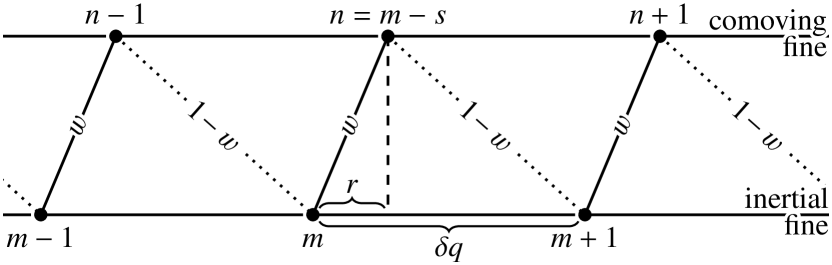
Figure 18: Linear interpolation on an infinite grid of knots separated by equidistant intervals $\delta q$. Each knot $n$ in the comoving frame (top line) is interpolated on the ${[m,m+1)}$ interval in the inertial frame (bottom line). The integer shift $s=m-n$ defines how many $\delta q$ intervals the comoving grid is Doppler-shifted with respect to the inertial grid. The l.h.s. $\varw$ and r.h.s. $1-\varw$ weights are indicated by sloped solid and dotted lines. The weight $\varw$ is determined by the remainder $r=q_{\mu}+q[n]-q[m]$, which is the frequency displacement between the inertial knot $m$ and its related comoving knot $n$.

Data: Line frequencies $q[i_{\mathrm{red}}{:}i_{\mathrm{blue}}]$, directions $\@vec{n}[1{:}N_{\mu}]$, velocities $\@vec{\varv}[x_{\mathrm{min}}{:}x_{\mathrm{max}},y_{\mathrm{min}}{:}y_{\mathrm{max}},z_{\mathrm{min}}{:}z_{\mathrm{max}}]$.

Result: Arrays shift and weight.

for $z\leftarrow z_{\mathrm{min}}$ to $z_{\mathrm{max}}$ do

      for $y\leftarrow y_{\mathrm{min}}$ to $y_{\mathrm{max}}$ do

           for $x\leftarrow x_{\mathrm{min}}$ to $x_{\mathrm{max}}$ do

                for $\mu\leftarrow 1$ to $N_{\mu}$ do

                     $q_{\mu}\leftarrow\bigl{(}\@vec{n}[\mu]\cdot\@vec{\varv}[x,y,z]\bigr{)}/\varv_{\mathrm{B}}$

                     $s\leftarrow\bigg{\lfloor}\dfrac{q_{\mu}}{\delta q}\bigg{\rfloor}$

                      // Integer shift between the two grids.

                     $r\leftarrow q_{\mu}-s\cdot\delta q$

                      // Fractional remainder.

                     $\varw\leftarrow 1-\dfrac{r}{\delta q}$

                      // The l.h.s. weight

                     $\mathmakebox[\widthof{$\mathtt{weight}$}][l]{\mathtt{shift}}[x,y,z,\mu]\leftarrow s$

                      // Store shift and weight.

                     $\mathtt{weight}[x,y,z,\mu]\leftarrow\varw$

                    

               

          

     

Alg. 7 Precomputation for equidistant interpolation.

At each grid point $(x,y,z)$, for each direction $\@vec{n}[\mu]$, we compute the Doppler shift $q_{\mu}$. The comoving knots $n$ are Doppler-shifted along the inertial knots $m$ by $s$ intervals of $\delta q$ length and a fractional remainder $r$ such that

$$q_{\mu}=s\cdot\delta q+r.$$ (53)

If inertial knot $m$ has a comoving nearest-right neighbor knot $n$, then $m-n=s$. The frequency displacement between these knots is $q_{\mu}+q[n]-q[m]=r$. The remainder $r$ determines the interpolation weights for the comoving knot $n$ on the inertial interval ${[m,m+1)}$. The l.h.s. weight is

$$\varw=\frac{\delta q-r}{\delta q}=1-\frac{r}{\delta q}.$$ (54)

There are three advantages of using equidistant frequency grids. First, for a given index tuple $(x,y,z,\mu)$, the values of $s$, $r$, and $\varw$ are independent of frequency as illustrated in Fig. 18. Second, during the transforms, we can limit the searching range for comoving knots by using the $m=n+s$ relation. Third, both the forward and backward transforms use the same values of $s$ and $\varw$. Therefore, we precompute and store $s$ and $\varw$ in two 4D-arrays (shift and weight) following Alg. 7.

A.5.2 Equidistant forward transform

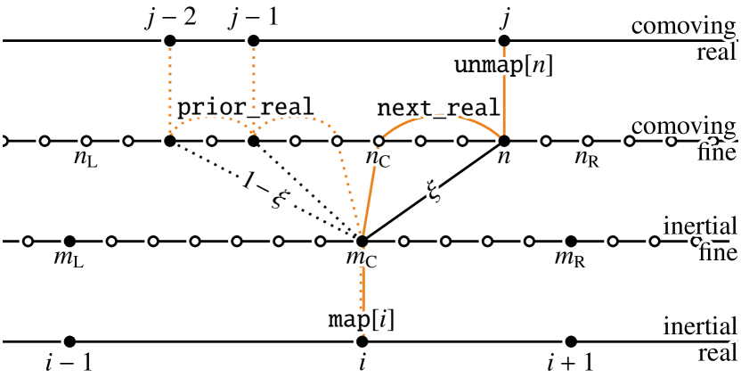
Figure 19: Equidistant forward interpolation from the inertial real grid onto the comoving real grid using the fine grids. Real knots $(\bullet)$ are marked on the real and the fine grids; virtual knots $(\circ)$ are marked on the fine grids. Knots $i-1$, $i$, and $i+1$ are projected from the inertial real onto inertial fine grid using the map array ($m_{\mathrm{L}}$, $m_{\mathrm{C}}$, $m_{\mathrm{R}}$) and corrected for the shift $s$ to obtain the corresponding nearest-right neighbors $n_{\mathrm{L}}$, $n_{\mathrm{C}}$, and $n_{\mathrm{R}}$ in the comoving fine grid. In the comoving fine grid, two scans with running index $n$ are done to find real knots on the intervals ${[m_{\mathrm{L}},m_{\mathrm{C}}]}$ and ${[m_{\mathrm{C}},m_{\mathrm{R}}]}$: from $n_{\mathrm{C}}$ to $n_{\mathrm{R}}-1$ using the next_real array (solid orange line), and from $n_{\mathrm{C}}-1$ to $n_{\mathrm{L}}$ using the prior_real array (dotted orange line). When a real knot is found, we find the corresponding real comoving grid index $j$ using the unmap array. The desired l.h.s. $\xi$ (sloped black solid line) or r.h.s. $1-\xi$ (sloped black dotted line) weights are computed from $n$, $n_{\mathrm{L}}$, $n_{\mathrm{C}}$, $n_{\mathrm{R}}$, and $\varw$.

Data: Specific intensity $I[x,y,z,\mu,i]$ at frequency $q[i]$ and direction $\@vec{n}[\mu]$ in the inertial frame.

Result: Incremented angle-averaged intensity $J^{\star\!}[x,y,z,j]$ at corresponding frequencies $q[j]$ in the comoving frame.

$n_{\mathrm{max}}\leftarrow\mathrm{size}(\mathtt{map})$ // Fine grid length.

$\mathmakebox[\widthof{$\varw$}][l]{s}\leftarrow\mathmakebox[\widthof{$\mathtt{weight}$}][l]{\mathtt{shift}}[x,y,z,\mu]$

$\varw\leftarrow\mathtt{weight}[x,y,z,\mu]$

$n_{\mathrm{L}}\leftarrow\mathtt{map}\mathmakebox[\widthof{$[\min(i_{\mathrm{blue}},i+1)]$}][l]{\bigl{[}\max(i-1,i_{\mathrm{red}})\bigr{]}}-s$ // Nearest-right neighbors of

$n_{\mathrm{C}}\leftarrow\mathtt{map}\mathmakebox[\widthof{$[\min(i_{\mathrm{blue}},i+1)]$}][l]{\bigl{[}i\bigr{]}}-s$ // $i-1$, $i$, and $i+1$ on the fine

$n_{\mathrm{R}}\leftarrow\mathtt{map}\bigl{[}\min(i_{\mathrm{blue}},i+1)\bigr{]}-s$ // grid in the comoving frame.

if $n_{\mathrm{L}}\neq n_{\mathrm{C}}$ then // Linear interpolation on ${[i-1,i)}$:

      $n\leftarrow\min\bigl{(}n_{\mathrm{C}}-1,n_{\mathrm{max}}\bigr{)}$

      if $1\leq n$ then

           if not $\mathtt{real\_knot}[n]$ then $n\leftarrow\mathtt{prior\_real}[n]$

           while $\max\bigl{(}1,n_{\mathrm{L}}\bigr{)}\leq n$ do

                $\xi^{\prime}\leftarrow\dfrac{n-n_{\mathrm{L}}+1-\varw}{n_{\mathrm{C}}-n_{\mathrm{L}}}$ // The r.h.s. weight.

                $J^{\star\!}\bigl{[}x,y,z,\mathtt{unmap}[n]\bigr{]}\overset{+}{\leftarrow}\xi^{\prime}\dfrac{\omega_{\mu}}{4\pi}I[x,y,z,\mu,i]$

                $n\leftarrow\mathtt{prior\_real}[n]$

               

          

     

else $n_{\mathrm{L}}=n_{\mathrm{C}}$ // Constant extrapolation on ${({-}\infty,i_{\mathrm{red}})}$:

      $n\leftarrow\min\bigl{(}n_{\mathrm{C}}-1,n_{\mathrm{max}}\bigr{)}$

      if $1\leq n$ then

           if not $\mathtt{real\_knot}[n]$ then $n\leftarrow\mathtt{prior\_real}[n]$

           while $1\leq n$ do

                $J^{\star\!}\bigl{[}x,y,z,\mathtt{unmap}[n]\bigr{]}\overset{+}{\leftarrow}\dfrac{\omega_{\mu}}{4\pi}I[x,y,z,\mu,i]$

                $n\leftarrow\mathtt{prior\_real}[n]$

               

          

     

if $n_{\mathrm{C}}\neq n_{\mathrm{R}}$ then // Linear interpolation on ${[i,i+1)}$:

      $n\leftarrow\max\bigl{(}1,n_{\mathrm{C}}\bigr{)}$

      if $n\leq n_{\mathrm{max}}$ then

           if not $\mathtt{real\_knot}[n]$ then $n\leftarrow\mathtt{next\_real}[n]$

           while $n\leq\min\bigl{(}n_{\mathrm{R}}-1,n_{\mathrm{max}}\bigr{)}$ do

                $\xi\leftarrow\dfrac{n_{\mathrm{R}}-n-(1-\varw)}{n_{\mathrm{R}}-n_{\mathrm{C}}}$ // The l.h.s. weight.

                $J^{\star\!}\bigl{[}x,y,z,\mathtt{unmap}[n]\bigr{]}\overset{+}{\leftarrow}\xi\dfrac{\omega_{\mu}}{4\pi}I[x,y,z,\mu,i]$

                $n\leftarrow\mathtt{next\_real}[n]$

               

          

     

else $n_{\mathrm{C}}=n_{\mathrm{R}}$ // Constant extrapolation on ${[i_{\mathrm{blue}},{+}\infty)}$:

      $n\leftarrow\max\bigl{(}1,n_{\mathrm{C}}\bigr{)}$

      if $n\leq n_{\mathrm{max}}$ then

           if not $\mathtt{real\_knot}[n]$ then $n\leftarrow\mathtt{next\_real}[n]$

           while $n\leq n_{\mathrm{max}}$ do

                $J^{\star\!}\bigl{[}x,y,z,\mathtt{unmap}[n]\bigr{]}\overset{+}{\leftarrow}\dfrac{\omega_{\mu}}{4\pi}I[x,y,z,\mu,i]$

                $n\leftarrow\mathtt{next\_real}[n]$

               

          

     

Alg. 8 Equidistant forward transform.

The forward transform for the equidistant grid is given by Alg. 8. Figure 19 provides an illustration.

Interpolation is performed on the fine grid. We project the current knot $i$ and its left $i-1$ and right $i+1$ neighbors from the inertial real grid onto the inertial fine grid:

$$m_{\mathrm{L}} =\mathtt{map}\bigl{[}\max(i-1,i_{\mathrm{red}})\bigr{]},$$ (55)

$$m_{\mathrm{C}} =\mathtt{map}\bigl{[}i\bigr{]},$$ (56)

$$m_{\mathrm{R}} =\mathtt{map}\bigl{[}\min(i_{\mathrm{blue}},i+1)\bigr{]}.$$ (57)

We use $\max(i-1,i_{\mathrm{red}})$ and $\min(i_{\mathrm{blue}},i+1)$ to avoid going beyond the profile ends $i=i_{\mathrm{red}}$ and $i=i_{\mathrm{blue}}$.

Indices of the related nearest-right neighbors in the comoving fine grid are computed from the shift $s$:

$$n_{\mathrm{L}}=\mathtt{map}\bigl{[}\max(i-1,i_{\mathrm{red}})\bigr{]} {}-s,$$ (58)

$$n_{\mathrm{C}}=\mathtt{map}\bigl{[}i\bigr{]} {}-s,$$ (59)

$$n_{\mathrm{R}}=\mathtt{map}\bigl{[}\min(i_{\mathrm{blue}},i+1)\bigr{]} {}-s.$$ (60)

To interpolate on the ${[i,i+1)}$ interval, we scan the comoving fine grid knots $n_{\mathrm{C}},\dotsc,n_{\mathrm{R}}-1$ that lie on the ${[m_{\mathrm{C}},m_{\mathrm{R}}]}$ interval.

Moving from $n=n_{\mathrm{C}}$ to $n_{\mathrm{R}}-1$, we look for real knots. If $n$ is a virtual knot, we jump to the next real knot using the next_real array. If $n$ is a real knot, we find the corresponding index $j$ in the comoving real grid using the unmap array. Then the desired l.h.s. weight $\xi$ is computed from $n$, $n_{\mathrm{C}}$, $n_{\mathrm{R}}$, and the fine grid weight $\varw$:

$$\xi=\dfrac{n_{\mathrm{R}}-n-(1-\varw)}{n_{\mathrm{R}}-n_{\mathrm{C}}}.$$ (61)

To interpolate on the ${[i-1,i)}$ interval, we scan the comoving fine grid knots $n_{\mathrm{L}},\dotsc,n_{\mathrm{C}}-1$ that lie on the ${[m_{\mathrm{L}},m_{\mathrm{C}}]}$ interval. Moving from $n=n_{\mathrm{C}}-1$ to $n_{\mathrm{L}}$ we look for real knots. If $n$ is a virtual knot, we jump to the prior real knot using the prior_real array. If $n$ is a real knot, we find the corresponding index $j$ in the comoving real grid using the unmap array. The desired r.h.s. weight $1-\xi$ is then computed as

$$\xi^{\prime}\equiv 1-\xi=\dfrac{n-n_{\mathrm{L}}+1-\varw}{n_{\mathrm{C}}-n_{\mathrm{L}}}.$$ (62)

Extrapolation at the $i=i_{\mathrm{red}}$ or $i=i_{\mathrm{blue}}$ ends is done likewise.

In all four cases, we truncate the running index $n$ by taking $\max(1,n)$ or $\min(n,n_{\mathrm{max}})$ to keep it within the fine grid range $1,\dotsc,n_{\mathrm{max}}$.

A.5.3 Equidistant backward transform

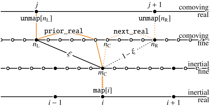
Figure 20: Equidistant backward interpolation from the comoving real grid onto the inertial real grid using the two fine grids. Real knots $(\bullet)$ are marked on the real and the fine grids; virtual knots $(\circ)$ are marked on the fine grid. The inertial real knot $i$ is projected onto the inertial fine grid using the map array ($m_{\mathrm{C}}$), and corrected for the shift $s$ to obtain the related nearest-right neighbor $n_{\mathrm{C}}$ in the comoving fine grid. If $n_{\mathrm{C}}<1$ or $n_{\mathrm{max}}\leq n_{\mathrm{C}}$, then constant extrapolation is done. If $n_{\mathrm{C}}$ is an internal knot, then we set $n_{\mathrm{L}}=n_{\mathrm{C}}-1$ and $n_{\mathrm{R}}=n_{\mathrm{C}}$ and check whether they both are real. If not, we find the nearest real knots using prior_real (indicated by the solid orange curve) or next_real (indicated by the orange dotted curve). Then $n_{\mathrm{L}}$ and $n_{\mathrm{R}}$ are projected onto the comoving real grid to get the corresponding knots $j$ and $j+1$. The desired l.h.s. $\xi$ (sloped solid black line) and r.h.s. $1-\xi$ (sloped dotted black line) weights are computed using $n_{\mathrm{L}}$, $n_{\mathrm{C}}$, $n_{\mathrm{R}}$, and $\varw$.

Data: Profile ratio $\rho^{\star\!}[x,y,z,j]$ for all frequencies $q[j]\colon j=j_{\mathrm{red}},\dotsc,j_{\mathrm{blue}}$ in the comoving frame.

Result: Profile ratio $\rho[x,y,z,\mu,i]$ at given frequency $q[i]$ and direction $\@vec{n}[\mu]$ in the inertial frame.

$n_{\mathrm{max}}\leftarrow\mathrm{size}(\mathtt{map})$ // Fine grid length.

$\mathmakebox[\widthof{$\varw$}][l]{s}\leftarrow\mathmakebox[\widthof{$\mathtt{weight}$}][l]{\mathtt{shift}}[x,y,z,\mu]$

$\varw\leftarrow\mathtt{weight}[x,y,z,\mu]$

$n_{\mathrm{C}}\leftarrow\mathtt{map}[i]-s$

  // Nearest-right neighbor of $i$ on the

  // fine grid in the comoving frame.

if $1<n_{\mathrm{C}}\leq n_{\mathrm{max}}$ then // Linear interpolation on ${[j,j+1)}$:

      $n_{\mathrm{L}}\leftarrow n_{\mathrm{C}}-1$

       // Nearest-left and right neighbors

      $n_{\mathrm{R}}\leftarrow n_{\mathrm{C}}$

       // in the comoving fine grid.

      if not $\mathtt{real\_knot}[n_{\mathrm{L}}]$ then $n_{\mathrm{L}}\leftarrow\mathtt{prior\_real}[n_{\mathrm{L}}]$

      if not $\mathtt{real\_knot}[n_{\mathrm{R}}]$ then $n_{\mathrm{R}}\leftarrow\mathtt{next\_real\ \,}[n_{\mathrm{R}}]$

      $\xi\leftarrow\dfrac{n_{\mathrm{R}}-n_{\mathrm{C}}+1-\varw}{n_{\mathrm{R}}-n_{\mathrm{L}}}$ // The l.h.s. weight.

     

       // Interpolate on the comoving grid:

      $\rho[x,y,z,\mu,i]\leftarrow\xi\,\rho^{\star\!}\bigl{[}x,y,z,\mathtt{unmap}[n_{\mathrm{L}}]\bigr{]}$

      $\mspace{57.0mu}{}+(1-\xi)\,\rho^{\star\!}\bigl{[}x,y,z,\mathtt{unmap}[n_{\mathrm{R}}]\bigr{]}$

     

else if $n_{\mathrm{max}}<n_{\mathrm{C}}$ then // Constant extrapolation on ${[j_{\mathrm{blue}},{+}\infty)}$:

      $\rho[x,y,z,\mu,i]\leftarrow\rho^{\star\!}[x,y,z,j_{\mathrm{blue}}]$

     

else $n_{\mathrm{C}}\leq 1$ // Constant extrapolation on ${({-}\infty,j_{\mathrm{red}})}$:

      $\rho[x,y,z,\mu,i]\leftarrow\rho^{\star\!}[x,y,z,j_{\mathrm{red}}]$

     

Alg. 9 Equidistant backward transform.

The backward interpolation employs the same ideas as the equidistant forward interpolation. It is given in Alg. 9 and illustrated in Fig. 20.

The current knot $i$ is projected from the inertial real onto the inertial fine grid using the map array to get $m_{\mathrm{C}}$. Then we compute its nearest-right neighbor $n_{\mathrm{C}}=m_{\mathrm{C}}-s$ in the comoving grid.

We test whether $n_{\mathrm{C}}$ is beyond the fine grid ends 1 or $n_{\mathrm{max}}$. If so, then we extrapolate from the comoving real grid ends $j_{\mathrm{red}}$ or $j_{\mathrm{blue}}$.

If not, then knot $i$ lies between knots $n_{\mathrm{C}}-1$ and $n_{\mathrm{C}}$. We set $n_{\mathrm{L}}=n_{\mathrm{C}}-1$ and $n_{\mathrm{R}}=n_{\mathrm{C}}$. If $n_{\mathrm{L}}$ or $n_{\mathrm{R}}$ are virtual, we use prior_real or next_real to set them to the nearest real knots.

Then we project $n_{\mathrm{L}}$ and $n_{\mathrm{R}}$ onto the comoving real grid using the unmap array to get the comoving real knots $j$ and $j+1$. The desired l.h.s. weight is computed using $n_{\mathrm{L}}$, $n_{\mathrm{C}}$, $n_{\mathrm{R}}$, and $\varw$:

$$\xi=\dfrac{n_{\mathrm{R}}-n_{\mathrm{C}}+1-\varw}{n_{\mathrm{R}}-n_{\mathrm{L}}}.$$ (63)