Ginzburg – Landau Expansion in BCS – BEC Crossover Region of Disordered Attractive Hubbard Model

Abstract

We have studied disorder effects on the coefficients of Ginzburg – Landau (GL) expansion for attractive Hubbard model within the generalized DMFT+$\Sigma$ approximation for the wide region of the values of attractive potential $U$ — from the weak-coupling limit, where superconductivity is described by BCS model, towards the strong coupling, where superconducting transition is related to Bose – Einstein condensation (BEC) of compact Cooper pairs.

For the case of semi-elliptic initial density of states disorder influence on the coefficients $A$ and $B$ before the square and the fourth power of the order parameter is universal for at all values of electronic correlations and is related only to the widening of the initial conduction band (density of states) by disorder. Similar universal behavior is valid for superconducting critical temperature $T_{c}$ (the generalized Anderson theorem) and specific heat discontinuity at the transition.

This universality is absent for the coefficient $C$ before the gradient term, which in accordance with the standard theory of “dirty” superconductors is strongly suppressed by disorder in the weak-coupling region, but can slightly grow in BCS – BEC crossover region, becoming almost independent of disorder in the strong coupling region. This leads to rather weak disorder dependence of the penetration depth and coherence length, as well as the slope of the upper critical magnetic field at $T_{c}$, in BCS – BEC crossover and strong coupling regions.

PACS:71.10.Fd, 74.20.-z, 74.20.Mn

I Introduction

Ilya Mikhailovich Lifshitz was one of the creators of the modern theory of disordered systems IML . Among his numerous contributions in this field we only mention the general formulation of the concept of self – averaging IML_UFN and the method of optimal fluctuation for the description of “Lifshitz tails” in the electron density of states IML_JETP . These ideas and approaches are widely used now in many fields of the theory of disordered systems, even those which initially were outside the scope of his personal scientific interests.

The studies of disorder effects in superconductors have a rather long history. The pioneer works by Abrikosov and Gor’kov AG_impr ; AG_imp ; AG_mimp and Anderson And_th had been devoted to the limit of weakly disordered metal ($p_{F}l\gg 1$, where $p_{F}$ is Fermi momentum and $l$ is the mean free path) and weakly coupled superconductors, well described by BCS theory Genn . The notorious Anderson theorem And_th ; Genn on $T_{c}$ of superconductors with “normal” (spin independent) disorder was proved in this limit under the assumption of self – averaging superconducting order – parameter Genn ; SCLoc_PRep ; SCLoc . The generalizations for the case of strong enough disorder ($p_{F}l\sim 1$) were also mainly done under the same assumption, though it can be explicitly shown, that self – averaging of the order parameter is violated close to Anderson metal – insulator transition SCLoc_PRep ; SCLoc . Here, the ideas originating from Ref. IML_JETP are of primary importance SadBul87 .

The problem of superconductivity in disordered systems in the limit of strongly coupled Cooper pairs, including the region of BCS – BEC crossover, was not well studied until recently. In fact, the problem of superconductivity in the case of strong enough pairing interactions was considered for a long enough time Leggett . Significant progress here was achieved by Nozieres and Schmitt-Rink NS , who proposed an effective method to study the crossover from BCS behavior in the weak coupling region towards Bose – Einstein condensation of Cooper pairs in the strong coupling region. One of the simplest models, where we can study the BCS – BEC crossover, is Hubbard model with attractive interaction. The most successful theoretical approach to describe strong electronic correlations in Hubbard model (both repulsive and attractive) is the dynamical mean field theory (DMFT) pruschke ; georges96 ; Vollh10 . The attractive Hubbard model was already studied within this approach in a number of papers Keller01 ; Toschi04 ; Bauer09 ; Koga11 ; JETP14 . However, there are only few papers, where disorder effects in BCS – BEC crossover region were taken into account.

In recent years we have developed the generalized DMFT+$\Sigma$ approach to Hubbard model JTL05 ; PRB05 ; FNT06 ; UFN12 , which is very convenient for the studies of different “external” (with respect to DMFT) interactions, such as pseudogap fluctuations JTL05 ; PRB05 ; FNT06 , disorder scattering HubDis ; HubDis2 and electron – phonon interaction e_ph_DMFT ). This approach is also well suited to the analysis of two – particle properties, such as dynamic (optical) conductivity HubDis ; PRB07 . In Ref. JETP14 we have used this approach to analyze the single – particle properties of the normal (non – superconducting) phase and optical conductivity of the attractive Hubbard model. Further on, DMFT+$\Sigma$ approach was used to study disorder influence on superconducting transition temperature, which was calculated within Nozieres – Schmitt-Rink approach JTL14 ; JETP15 .

The general review of DMFT+$\Sigma$ approach was given in Ref. UFN12 , and the review of this approach to disordered Hubbard model (both repulsive and attractive) was recently presented in Ref. JETP16_rev .

In this paper we investigate Ginzburg – Landau (GL) expansion for disordered attractive Hubbard model including the BCS – BEC crossover region and the limit of strong coupling. Coefficients of GL – expansion in BCS – BEC crossover region were studied in a number of papers Micnas01 ; Zwerger92 ; Zwerger97 , but there were no previous studies of disorder effects, except our recent paper JETP16 , where we have considered only the case of homogeneous GL – expansion and demonstrated certain universal behavior of GL – coefficients on disorder (reflecting the generalized Anderson theorem). Below we mainly concentrate on the study of the GL – coefficient before the gradient term, where such universal behavior is just absent. Here we limit ourselves to the case of weak enough disorder ($p_{F}l\gg 1$), neglecting the effects of Anderson localization, which can significantly change the behavior of this coefficient in the limit of strong disorder SCLoc_PRep ; SCLoc .

II Hubbard model within DMFT+$\Sigma$ approach

We shall consider the disordered paramagnetic Hubbard model with attractive interaction. The Hamiltonian is written as:

$$H=-t\sum_{\langle ij\rangle\sigma}a_{i\sigma}^{\dagger}a_{j\sigma}+\sum_{i\sigma}\epsilon_{i}n_{i\sigma}-U\sum_{i}n_{i\uparrow}n_{i\downarrow},$$ (1)

where $t>0$ is the transfer integral between the nearest neighbors on the lattice, $U$ is the Hubbard – like on site attraction, $n_{i\sigma}=a_{i\sigma}^{\dagger}a_{i\sigma}^{{\phantom{\dagger}}}$ is electron number operator at site $i$, $a_{i\sigma}$ ($a_{i\sigma}^{\dagger}$) is electron annihilation (creation) operator at $i$-th site and spin $\sigma$. Local energy levels $\epsilon_{i}$ are assumed to be independent and random at different sites. To use the standard “impurity” diagram technique we assume the Gaussian statistics for energy levels $\epsilon_{i}$:

$$\mathcal{P}(\epsilon_{i})=\frac{1}{\sqrt{2\pi}\Delta}\exp\left(-\frac{\epsilon_{i}^{2}}{2\Delta^{2}}\right)$$ (2)

Parameter $\Delta$ here is the measure of disorder strength, while the Gaussian random field of energy levels introduces the “impurity” scattering, which is considered using the standard approach, using the averaged Green’s functions Diagr .

The generalized DMFT+$\Sigma$ approach JTL05 ; PRB05 ; FNT06 ; UFN12 adds to the standard DMFT pruschke ; georges96 ; Vollh10 an additional “external” electron self – energy $\Sigma_{\bf p}(\varepsilon)$ (in general case momentum dependent), which is produced by additional interactions outside the DMFT, which gives an effective procedure to calculate both single – particle and two – particle properties HubDis ; PRB07 ; JETP16_rev . The success of this approach is related to choice of the single – particle Green’s function in the following form:

$$G(\varepsilon,{\bf p})=\frac{1}{\varepsilon+\mu-\varepsilon({\bf p})-\Sigma(\varepsilon)-\Sigma_{\bf p}(\varepsilon)},$$ (3)

where $\varepsilon({\bf p})$ – is the “bare” electron dispersion, while the full self – energy is the additive sum the local self – energy $\Sigma(\varepsilon)$, determined from DMFT, and “external” $\Sigma_{\bf p}(\varepsilon)$. Thus we neglect all the interference processes between of Hubbard and “external” interactions. This allows us to conserve the general structure of self – consistent equations of the standard DMFT pruschke ; georges96 ; Vollh10 . At the same time, at each step of DMFT iterations the “external” self – energy $\Sigma_{\bf p}(\varepsilon)$ is recalculated using some approximate calculation scheme, corresponding to the form of additional interaction, while the local Green’s function is dressed by $\Sigma_{\bf p}(\varepsilon)$ at each step of DMFT procedure.

Here, in the impure Hubbard model, the “external” self – energy entering DMFT+$\Sigma$ is taken in the simplest form (self – consistent Born approximation), which neglects all diagrams with intersecting lines of impurity scattering, so that:

$$\Sigma_{\bf p}(\varepsilon)\to\tilde{\Sigma}(\varepsilon)=\Delta^{2}\sum_{\bf p}G(\varepsilon,{\bf p}),$$ (4)

where $G(\varepsilon,{\bf p})$ is the single – electron Green’s function (3) and $\Delta$ is the amplitude of site disorder.

To solve the effective Anderson impurity model of DMFT throughout this paper we used the numerical renormalization group (NRG) algorithm NRGrev . All calculations below were done for the case of the quarter – filled band (n=0.5 electrons per lattice site).

Further on we shall consider the model of the “bare” conduction band with semi – elliptic density of states (per unit cell and single spin projection):

$$N_{0}(\varepsilon)=\frac{2}{\pi D^{2}}\sqrt{D^{2}-\varepsilon^{2}}$$ (5)

where $D$ defines the band half – width. This is a rather good approximation for three – dimensional case.

In Ref. JETP15 we have given an analytic proof that in DMFT+$\Sigma$ approximation for disordered Hubbard model with semi – elliptic density of states all disorder effects in single – particle properties, calculated in DMFT+$\Sigma$ (with the use of self – consistent Born approximation (4)) are reduced to conduction band – widening by disorder, i.e. to the replacement (in the density of states) $D\to D_{eff}$, where $D_{eff}$ is the effective half – width of the band in the presence of disorder scattering:

$$D_{eff}=D\sqrt{1+4\frac{\Delta^{2}}{D^{2}}}.$$ (6)

so that the “bare” density of states (in the absence of correlations,$U=0$) becomes:

$$\tilde{N}_{0}(\xi)=\frac{2}{\pi D_{eff}^{2}}\sqrt{D_{eff}^{2}-\varepsilon^{2}}$$ (7)

conserving its semi – elliptic form. It should be noted, that for different models of the “bare” conduction band disorder can also change the form of the density of states, so that such universal disorder effects in single – properties is absent. However, in the limit of strong enough disorder almost any initial density of states actually acquires semi – elliptic form, restoring this universal dependence on disorder JETP15 .

The temperature of superconducting transition in attractive Hubbard model within DMFT was calculated in a number of papers Keller01 ; Toschi04 ; Koga11 , analyzing both from the Cooper instability of the normal phase Keller01 (divergence of Cooper susceptibility) and from the disappearance of superconducting order parameter Toschi04 ; Koga11 . In Ref. JETP14 we determined the critical temperature from instability of the normal phase (instability of DMFT iteration procedure). The results obtained were in good agreement with the results of Refs. Keller01 ; Toschi04 ; Koga11 . Besides that, in Ref. JETP14 to calculate $T_{c}$ we have used the Nozieres – Schmitt-Rink approach NS , showing that this approach allows qualitatively, though approximately, describes the BCS – BEC crossover region. In Refs. JTL14 ; JETP15 we used the combination of Nozieres – Schmitt-Rink approach and DMFT+$\Sigma$ for detailed studies of disorder influence on the temperature of superconducting transition and the number of local pairs. In this approach we determine $T_{c}$ from the following equation JETP15 :

$$1=\frac{U}{2}\int_{-\infty}^{\infty}d\varepsilon\tilde{N}_{0}(\varepsilon)\frac{th\frac{\varepsilon-\mu}{2T_{c}}}{\varepsilon-\mu}.$$ (8)

with chemical potential $\mu$ for different $U$ and $\Delta$ being determined from DMFT+$\Sigma$ calculations, i.e. from the standard equation for the number of electrons (band filling), defined by the Green’s function (3). This allows us to find $T_{c}$ for the wide range of the model parameters, including the BCS – BEC crossover region and the limit of strong coupling, as well as for the different disorder levels. This reflects the physical meaning of Nozieres – Schmitt-Rink approximation: in the weak coupling region transition temperature is controlled by the equation for Cooper instability (8), while in the strong coupling limit it is determined by the temperature of Bose condensation of compact Cooper pairs, which is controlled by chemical potential.

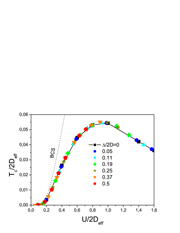
Figure 1: Universal dependence of superconducting critical temperature on Hubbard attraction for different levels of disorder.

In Fig. 1 we show the universal dependence of superconducting critical temperature $T_{c}$ on Hubbard attraction for different levels of disorder obtained in Ref. JETP15 . This is a manifestation of the generalized Anderson theorem. In the weak coupling region $T_{c}$ is well described by BCS model (dashed line in Fig. 1 shows $T_{c}$ determined by Eq. (8) with chemical potential independent of $U$ and obtained for the quarter – filled “bare” band), while in the strong coupling region $T_{c}$ is determined by the condition of Bose condensation of Cooper pairs giving $\sim t^{2}/U$ dependence (corresponding to inverse mass dependence of compact Bosons), passing through a characteristic maximum at $U/2D_{eff}\sim 1$ in BCS – BEC crossover region.

III Ginzburg – Landau expansion

Ginzburg – Landau expansion for the difference of free energies of superconducting and normal phases can be written in the standard form:

$$F_{s}-F_{n}=A|\Delta_{\bf q}|^{2}+q^{2}C|\Delta_{\bf q}|^{2}+\frac{B}{2}|\Delta_{\bf q}|^{4},$$ (9)

where $\Delta_{\bf q}$ is the Fourier component of the order parameter.

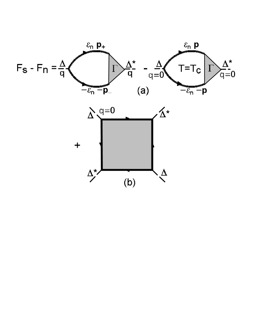
Figure 2: Diagrammatic representation of Ginzburg – Landau expansion.

Microscopically GL – expansion (9) is determined by diagrams of loop – expansion for the free energy of electrons in an “external” field of random fluctuations of order parameter with small wave – vector ${\bf q}$ SCLoc ; Diagr shown in Fig.2 (where fluctuations are represented by dashed lines). In disordered system, the use here of the standard impurity diagram technique implicitly assumes the self – averaging nature of the order parameter Genn ; SCLoc_PRep ; SCLoc .

Within the framework of Nozieres – Schmitt-Rink approach NS the loops with two and four Cooper vertices, shown in Fig.2, do not contain contributions from attractive Hubbard interaction (as in weak coupling theory) and are “dressed” only by disorder (impurity) scattering . However, the chemical potential here, which has an important dependence on the strength of interaction $U$ and determines the condition of Bose condensation of Cooper pairs, should be calculated in the framework of DMFT+$\Sigma$ approximation, as it was done in Refs. JTL14 ; JETP15 in calculations of $T_{c}$.

In Ref. JETP16 we have shown that in this approach GL – coefficients $A$ and $B$ are determined by the following expressions:

$$A(T)=\frac{1}{U}-\int_{-\infty}^{\infty}d\varepsilon\tilde{N}_{0}(\varepsilon)\frac{th\frac{\varepsilon-\mu}{2T}}{2(\varepsilon-\mu)},$$ (10)

$$B=\int_{-\infty}^{\infty}\frac{d\varepsilon}{2(\varepsilon-\mu)^{3}}\left(th\frac{\varepsilon-\mu}{2T}-\frac{(\varepsilon-\mu)/2T}{ch^{2}\frac{\varepsilon-\mu}{2T}}\right)\tilde{N}_{0}(\varepsilon),$$ (11)

For $T\to T_{c}$ coefficient $A(T)$ takes the usual form:

$$A(T)\equiv\alpha(T-T_{c}).$$ (12)

In BCS weak coupling limit we obtain the standard expressions for $\alpha$ and $B$ Diagr :

$$\alpha_{BCS}=\frac{\tilde{N}_{0}(\mu)}{T_{c}},\qquad B_{BCS}=\frac{7\zeta(3)}{8\pi^{2}T_{c}^{2}}\tilde{N}_{0}(\mu).$$ (13)

so that coefficients $A$ and $B$ are determined only by disorder widened density of states $\tilde{N}_{0}(\varepsilon)$ and chemical potential $\mu$. Then, in the case of semi – elliptic density of states their dependence on disorder is described by the simple replacement $D\to D_{eff}$ and we have universal dependencies of $\alpha$ and $B$ (properly normalized by powers of $2D_{eff}$) on $U/2D_{eff}$, as shown in Fig. 3. Both $\alpha$ and $B$ drop fast with the growth of interaction $U/2D_{eff}$.

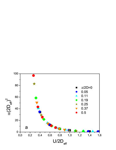
Figure 3: Universal dependence of Ginzburg – Landau coefficients $\alpha$ (a) and $B$ (b) on the strength of Hubbard attraction for different levels of disorder.

It should be noted that Eqs. (10) and (11) for coefficients $A$ and $B$ were obtained in Ref. JETP16 using the exact Ward identities and remain valid also in the limit of strong disorder (up to Anderson localization). Correspondingly, in the limit of strong disorder the coefficients $A$ and $B$ depend on disorder only via appropriate dependence of the density of states.

Dependence on disorder, related only to the band widening by $D\to D_{eff}$, is also observed for specific heat discontinuity at the critical temperature JETP16 , determined by coefficients $\alpha$ and $B$:

$$C_{s}(T_{c})-C_{n}(T_{c})=T_{c}\frac{\alpha^{2}}{B}.$$ (14)

In Fig. 4 we show the universal dependence of specific heat discontinuity on $U/2D_{eff}$. In BCS limit specific heat discontinuity grows with coupling, while in BEC limit it drops with $U/2D_{eff}$, passing through maximum at $U/2D_{eff}\approx 0.55$ in BCS – BEC crossover region. This behavior of specific heat discontinuity is mainly related to the similar dependence of $T_{c}$ (cf. Fig. 1), as $\frac{\alpha^{2}}{B}$ in Eq. (14) only smoothly depends on the coupling strength.

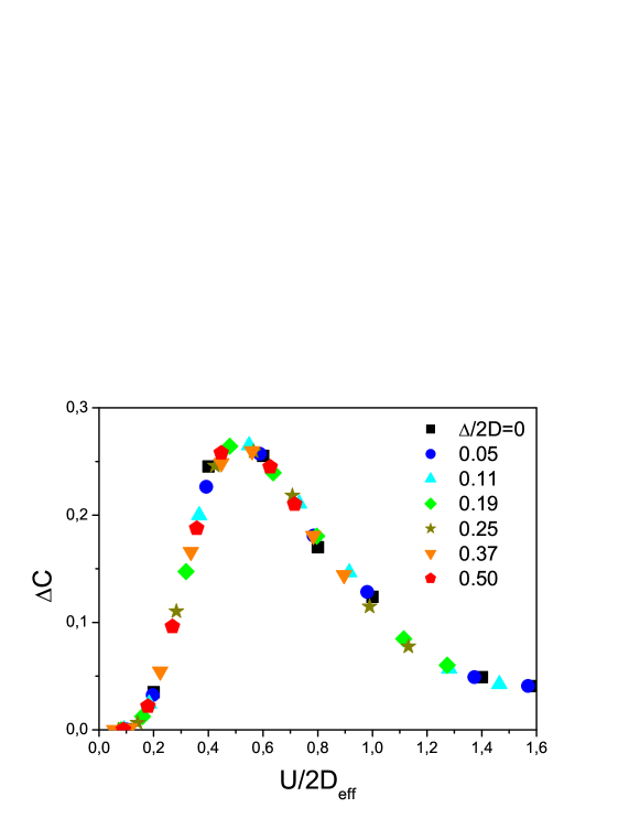
Figure 4: Universal dependence of specific heat discontinuity on $U/2D_{eff}$ for different disorder levels.

From diagrammatic representation of GL – expansion shown in Fig. 2 it is clear, that coefficient $C$ is determined by the $q^{2}$ term in the expansion of the two – particle loop (first term in Fig. 2) in powers of $q$. Then we obtain:

$$C=-T\lim_{q\to 0}\sum_{n,\bf p,\bf{p^{\prime}}}\frac{\Phi_{\bf p\bf{p^{\prime}}}(\varepsilon_{n},{\bf q})-\Phi_{\bf p\bf{p^{\prime}}}(\varepsilon_{n},0)}{q^{2}},$$ (15)

where $\Phi_{\bf p,\bf{p^{\prime}}}(\varepsilon_{n},{\bf q})$ is two – particle Green’s function in Cooper channel “dressed” (in Nozieres – Schmitt-Rink approximation) only by impurity scattering. To determine the coefficient $C$ we again use the exact Ward identity, derived by us in Ref. PRB07 :

$$G(\varepsilon_{n},{\bf p_{+}})-G(-\varepsilon_{n},-{\bf p_{-}})=-\sum_{\bf p^{\prime}}\Phi_{\bf pp^{\prime}}(\varepsilon_{n},{\bf q})\left[(G_{0}^{-1}(\varepsilon_{n},{\bf p^{\prime}_{+}})-G_{0}^{-1}(-\varepsilon_{n},-{\bf p^{\prime}_{-}})\right],$$ (16)

where ${\bf p_{\pm}}={\bf p}\pm\frac{\bf q}{2}$, $G_{0}(\varepsilon_{n},{\bf p})=\frac{1}{\varepsilon_{n}+\mu-\varepsilon_{\bf p}}$ is the “bare” single – particle Green’s function at Fermion Matsubara frequencies $\varepsilon_{n}$, while $G(\varepsilon_{n},{\bf p})$ is the single – particle Green’s function “dressed” only by impurity scattering. Introducing the notation $\Delta G(\varepsilon_{n},{\bf p})=G(\varepsilon_{n},{\bf p_{+}})-G(-\varepsilon_{n},-{\bf p_{-}})$ and using the symmetry $\varepsilon({\bf p})=\varepsilon(-{\bf p})$ and $G(\varepsilon_{n},-{\bf p})=G(\varepsilon_{n},{\bf p})$ we rewrite the Ward identity as:

$$\Delta G(\varepsilon_{n},{\bf p})=-\sum_{\bf p^{\prime}}\Phi_{\bf pp^{\prime}}(\varepsilon_{n},{\bf q})(2i\varepsilon_{n}-\Delta\varepsilon_{\bf p^{\prime}}),$$ (17)

where $\Delta\varepsilon_{\bf p}=\varepsilon_{\bf p_{+}}-\varepsilon_{\bf p_{-}}$. Then we can perform here summation over ${\bf p}$ (also with additional multiplication by $\Delta\varepsilon_{\bf p}$) to obtain the following system of equations:

$$\sum_{\bf{p}}\Delta G(\varepsilon_{n},{\bf p}) = -2i\varepsilon_{n}\Phi_{0}(\varepsilon_{n},{\bf q})+\Phi_{1}(\varepsilon_{n},{\bf q})$$

$$\sum_{\bf{p}}\Delta\varepsilon_{\bf p}\Delta G(\varepsilon_{n},{\bf p}) = -2i\varepsilon_{n}\Phi_{1}(\varepsilon_{n},{\bf q})+\sum_{\bf p,p^{\prime}}\Delta\varepsilon_{\bf p}\Phi_{\bf pp^{\prime}}(\varepsilon_{n},{\bf q})\Delta\varepsilon_{\bf p^{\prime}},$$ (18)

where $\Phi_{0}(\varepsilon_{n},{\bf q})=\sum_{\bf pp^{\prime}}\Phi_{\bf pp^{\prime}}(\varepsilon_{n},{\bf q})$, $\Phi_{1}(\varepsilon_{n},{\bf q})=\sum_{\bf pp^{\prime}}\Phi_{\bf pp^{\prime}}(\varepsilon_{n},{\bf q})\Delta\varepsilon_{\bf p^{\prime}}=\sum_{\bf pp^{\prime}}\Delta\varepsilon_{\bf p}\Phi_{\bf pp^{\prime}}(\varepsilon_{n},{\bf q})$. Then, excluding $\Phi_{1}(\varepsilon_{n},{\bf q})$ from this system of equations, we obtain:

$$\sum_{\bf{p}}\Delta\varepsilon_{\bf p}\Delta G(\varepsilon_{n},{\bf p})=-2i\varepsilon_{n}\sum_{\bf{p}}\Delta G(\varepsilon_{n},{\bf p})-(2i\varepsilon_{n})^{2}\Phi_{0}(\varepsilon_{n},{\bf q})+\sum_{\bf pp^{\prime}}\Delta\varepsilon_{\bf p}\Phi_{\bf pp^{\prime}}(\varepsilon_{n},{\bf q})\Delta\varepsilon_{\bf p^{\prime}}.$$ (19)

All terms in Eq. (19) are functions of ${\bf q}^{2}$. Let us write down two lowest – order terms of $q^{2}$ – expansion of Eq. (19). The $\sim q^{0}$ term is:

$$\Phi_{0}(\varepsilon_{n},{\bf q}=0)=-\frac{\sum_{\bf{p}}\Delta G(\varepsilon_{n},{\bf p})}{2i\varepsilon_{n}}.$$ (20)

As there is no dependence on the direction of ${\bf q}$ we choose ${\bf q}=(q,0,0)$. Then $\sim q^{2}$ terms are written as:

$$\varphi(\varepsilon_{n},{\bf q}=0){(2i\varepsilon_{n})}^{2}=\sum_{\bf{p}\bf{p^{\prime}}}v_{x}\Phi_{\bf{pp^{\prime}}}(\varepsilon_{n},{\bf q}){v_{x}}^{\prime}-\lim_{q\to 0}\frac{\sum_{\bf p}\Delta\varepsilon_{\bf p}\Delta G(\varepsilon_{n},{\bf p})}{q^{2}},$$ (21)

where $v_{x}=\frac{\partial\varepsilon_{\bf p}}{\partial p_{x}}$ and $\varphi(\varepsilon_{n},{\bf q}=0)=\lim_{q\to 0}\frac{\Phi_{0}(\varepsilon_{n},{\bf q})-\Phi_{0}(\varepsilon_{n},0)}{q^{2}}$.

For weak enough disorder we can neglect localization corrections and consider the two – particle loop in “ladder” approximation for disorder scattering. Then, due to vector nature of vertices, all vertex corrections vanish due to angular integration and we obtain:

$$\sum_{\bf{p}\bf{p^{\prime}}}v_{x}\Phi_{\bf{pp^{\prime}}}(\varepsilon_{n},{\bf q}){v_{x}}^{\prime}=\sum_{\bf p}{v_{x}}^{2}G(\varepsilon_{n},{\bf p})G(-\varepsilon_{n},{\bf p})$$ (22)

For the case of isotropic spectrum we have:

$$\lim_{q\to 0}\frac{\sum_{\bf p}\Delta\varepsilon_{\bf p}\Delta G(\varepsilon_{n},{\bf p})}{q^{2}}=-\frac{1}{2}\sum_{\bf p}\frac{{\partial}^{2}\varepsilon_{\bf p}}{\partial{p_{x}}^{2}}(G(\varepsilon_{n},{\bf p})+G(-\varepsilon_{n},{\bf p})).$$ (23)

As a result, we can write $C$ coefficient (15) as:

$$C=-T\sum_{n}\frac{\sum_{\bf p}{v_{x}}^{2}G(\varepsilon_{n},{\bf p})G(-\varepsilon_{n},{\bf p})+\frac{1}{2}\sum_{\bf p}\frac{{\partial}^{2}\varepsilon_{\bf p}}{\partial{p_{x}}^{2}}(G(\varepsilon_{n},{\bf p})+G(-\varepsilon_{n},{\bf p}))}{{(2i\varepsilon_{n})}^{2}}.$$ (24)

After the standard summation over Matsubara frequencies we obtain:

$$C=-\frac{1}{8\pi}\int_{-\infty}^{\infty}d\varepsilon\frac{th\frac{\varepsilon}{2T}}{\varepsilon}\sum_{\bf p}\left({v_{x}}^{2}Im\frac{G^{R}(\varepsilon,{\bf p})G^{A}(-\varepsilon,{\bf p})}{\varepsilon+i\delta}+\frac{{\partial}^{2}\varepsilon_{\bf p}}{\partial{p_{x}}^{2}}Im\frac{G^{R}(\varepsilon,{\bf p})}{\varepsilon+i\delta}\right).$$ (25)

Finally $C$ coefficient is expressed as:

$$C=-\frac{1}{8\pi}\int_{-\infty}^{\infty}d\varepsilon\frac{th\frac{\varepsilon}{2T}}{\varepsilon^{2}}\sum_{\bf p}\left({v_{x}}^{2}Im(G^{R}(\varepsilon,{\bf p})G^{A}(-\varepsilon,{\bf p}))+\frac{{\partial}^{2}\varepsilon_{\bf p}}{\partial{p_{x}}^{2}}ImG^{R}(\varepsilon,{\bf p})\right)+$$

$$\frac{1}{16T}\sum_{\bf p}\left({v_{x}}^{2}Re(G^{R}(0,{\bf p})G^{A}(0,{\bf p}))+\frac{{\partial}^{2}\varepsilon_{\bf p}}{\partial{p_{x}}^{2}}ReG^{R}(0,{\bf p})\right).$$ (26)

The procedure to calculate velocity $v_{x}$ and its derivative $\frac{{\partial}^{2}\varepsilon_{\bf p}}{\partial{p_{x}}^{2}}$ in the model with semi – elliptic density of states was discussed in detail in Ref. HubDis .

In the absence of disorder ($\Delta=0$) we replace $G\to G_{0}$ and the expression for $C$ takes the following form:

$$C=-\frac{1}{8\pi}\sum_{\bf p}\left(\frac{{v_{x}}^{2}}{{(\varepsilon_{\bf p}-\mu)}^{2}}-\frac{{\partial}^{2}\varepsilon_{\bf p}}{\partial{p_{x}}^{2}}\frac{1}{\varepsilon_{\bf p}-\mu}\right)\left(\frac{th\frac{\varepsilon_{\bf p}-\mu}{2T}}{\varepsilon_{\bf p}-\mu}-\frac{1}{2T}\right)$$ (27)

In the weak coupling BCS limit in the absence of disorder the coefficient $C$ reduces to the standard expression Diagr :

$$C_{BCS}=\frac{7\zeta(3)}{16\pi^{2}T_{c}^{2}}N_{0}(\mu)\frac{v_{F}^{2}}{d},$$ (28)

where $v_{F}$ is Fermi velocity, $d$ – dimensionality of space. Semi – elliptic density of states is a good approximation for $d=3$. As noted above disorder influence on $C$ is not reduced to a simple replacement $N_{0}\to\tilde{N}_{0}$, so that even in the BCS weak coupling limit (in contrast to coefficients $\alpha$ and $B$ (cf. (13)) we can not derive for $C$ a compact expression, similar to (28).

IV Main results

Let us discuss now the main results of our calculations for the gradient term coefficient $C$ of GL – expansion and the related physical characteristics, such as the coherence length, penetration depth and the slope of the upper critical magnetic field at $T_{c}$.

The coherence length at given temperature $\xi(T)$ determines the characteristic scale of order – parameter $\Delta$ inhomogeneities:

$$\xi^{2}(T)=-\frac{C}{A}.$$ (29)

Coefficient $A$ changes its sign at the critical temperature $A=\alpha(T-T_{c})$, so that

$$\xi(T)=\frac{\xi}{\sqrt{1-T/T_{c}}},$$ (30)

where we have introduced the coherence length as:

$$\xi=\sqrt{\frac{C}{\alpha T_{c}}}.$$ (31)

In the weak coupling limit and in the absence of disorder it is written in the standard form Diagr :

$$\xi_{BCS}=\sqrt{\frac{C_{BCS}}{\alpha_{BCS}T_{c}}}=\sqrt{\frac{7\zeta(3)}{16\pi^{2}d}}\frac{v_{F}}{T_{c}}.$$ (32)

Penetration depth of magnetic field into superconductor is defined as:

$$\lambda^{2}(T)=-\frac{c^{2}}{32\pi e^{2}}\frac{B}{AC}.$$ (33)

Thus:

$$\lambda(T)=\frac{\lambda}{\sqrt{1-T/T_{c}}},$$ (34)

where we have introduced:

$$\lambda^{2}=\frac{c^{2}}{32\pi e^{2}}\frac{B}{\alpha CT_{c}},$$ (35)

which in the absence of disorder has the form:

$$\lambda^{2}_{BCS}=\frac{c^{2}}{32\pi e^{2}}\frac{B_{BCS}}{\alpha_{BCS}C_{BCS}T_{c}}=\frac{c^{2}}{16\pi e^{2}}\frac{d}{N_{0}(\mu)v_{F}^{2}}.$$ (36)

Note that $\lambda_{BCS}$ does not depend on $T_{c}$, and correspondingly on the coupling strength, so that it is convenient for normalization of penetration depth $\lambda$ (35) for arbitrary $U$ and $\Delta$.

Close to $T_{c}$ the upper critical field $H_{c2}$ is defined via GL – coefficients as:

$$H_{c2}=\frac{\Phi_{0}}{2\pi\xi^{2}(T)}=-\frac{\Phi_{0}}{2\pi}\frac{A}{C},$$ (37)

where $\Phi_{0}=c\pi/e$ is magnetic flux quantum. Then the slope of the upper critical field at $T_{c}$ is given by:

$$\frac{dH_{c2}}{dT}=\frac{\Phi_{0}}{2\pi}\frac{\alpha}{C}.$$ (38)

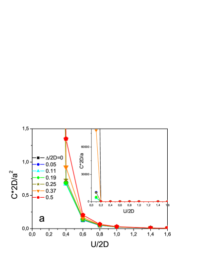
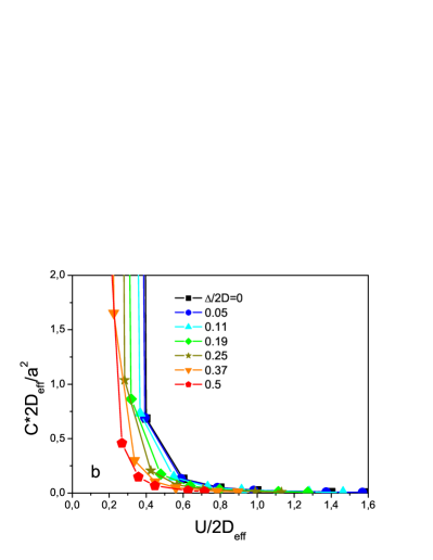
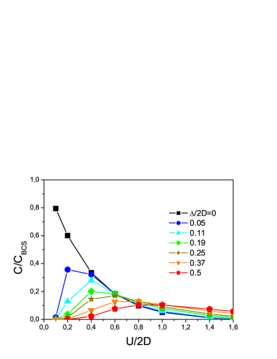
Figure 5: Dependence of the coefficient $C$ on the strength of Hubbard attraction for different levels of disorder ($a$ – lattice parameter). (a) — all energy units are normalized by the width of the “bare” conduction band $2D$. (b) — all energy units normalized by effective band width $2D_{eff}$. (c) — coefficient $C$ normalized by its value $C_{BCS}$ in the weak coupling limit and in the absence of disorder.

In Fig. 5 we show the dependencies of coefficient $C$ on the strength of Hubbard attraction for different disorder levels. It is seen that $C$ drops fast with the growth of the coupling constant. Especially fast this drop is in the weak coupling region (see insert in Fig. 5(a)). Being essentially a two – particle characteristic coefficient $C$ does not demonstrate universal dependencies on disorder, similar to $\alpha$ and $B$ coefficients, as is clearly seen from Fig. 5 (b). Fig. 5 (c) shows the coupling strength dependence of $C$ normalized by its BCS value (28) in the absence of disorder.

Figure 6: Dependence of coefficient $C$, normalized by its value in the absence of disorder, on disorder levels for different values of Hubbard attraction $U$.

In Fig. 6 we show the dependencies of $C$ on disorder for different values of coupling strength $U/2D$. In the weak coupling limit ($U/2D=0.1$) we observe fast enough drop of $C$ with the growth of disorder in the region of weak enough disorder scattering. However, in the region of strong enough disorder we can observe even the growth of $C$ with disorder, related mainly to noticeable band widening at high disorder levels and respective drop in the effective coupling $U/2D_{eff}$. For intermediate couplings ($U/2D=0.4-0.6$) coefficient $C$ only demonstrates some weak growth with disorder. In BEC limit ($U/2D>1$) coefficient $C$ is practically independent of disorder.

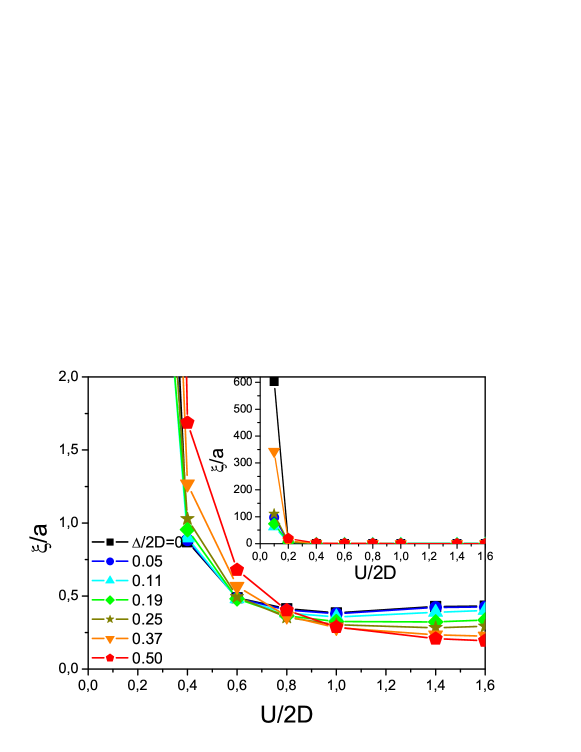
Figure 7: Dependence of coherence length, normalized by lattice parameter $a$, on Hubbard attraction $U$ for different disorder levels. Insert: fast growth of coherence length in weak coupling BCS limit.

Let us now discuss the physical characteristics. Dependence of coherence length on the strength of Hubbard attraction is shown in Fig. 7. We can see that in the weak coupling region (cf. insert in Fig.7) the coherence length drops fast with the growth of $U$ at any disorder level, reaching the values of the order of lattice spacing $a$ at the intermediate couplings $U/2D\sim 0.4-0.6$. The further growth of the coupling strength leads only to small changes of coherence length.

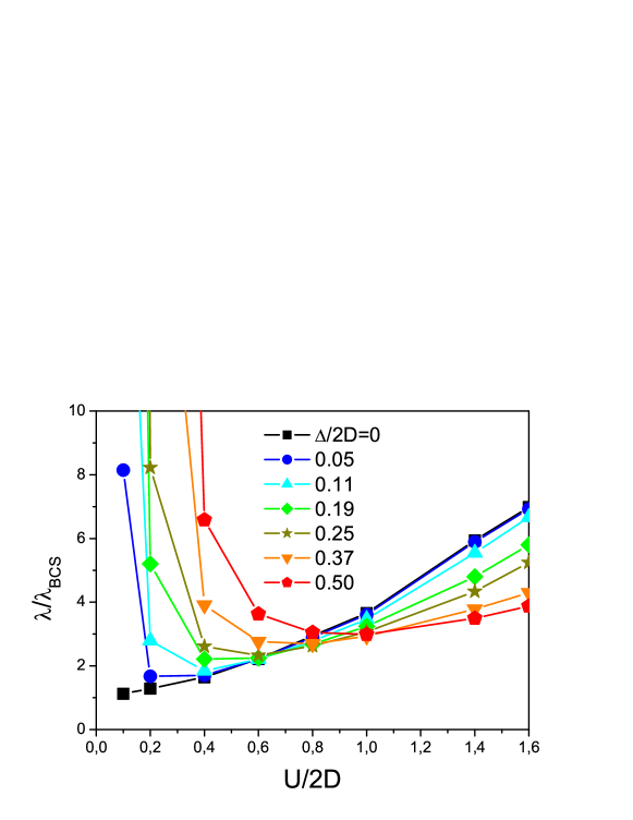
Figure 8: Dependence of penetration depth, normalized by its BCS value in the absence of disorder, on Hubbard attraction $U$ for different disorder levels.

In Fig. 8 we show the dependence of penetration depth, normalized by its BCS value in the absence of disorder (36), on Hubbard attraction $U$ for different levels of disorder. In the absence of disorder scattering penetration depth grows with coupling. Disorder in BCS weak coupling limit leads to fast growth of penetration depth (for “dirty” BCS superconductors $\lambda\sim l^{-1/2}$, where $l$ is the mean free path). In BEC strong coupling region disorder only slightly diminishes the penetration depth (cf. Fig. 11(a)).

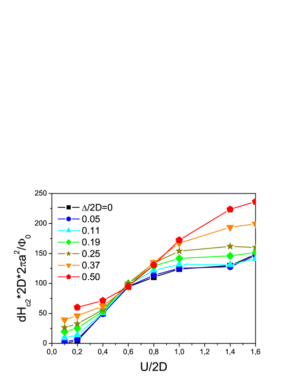
Figure 9: Dependence of the upper critical magnetic field slope on Hubbard attraction $U$ for different disorder levels.

Dependence of the slope of the upper critical filed $dH_{c2}\equiv(dH_{c2}/dT)_{T=T_{c}}$ on Hubbard attraction for different disorder levels is shown in Fig. 9. For any value of disorder scattering the slope of the upper critical field grows with coupling. However, in the limit of weak disorder we observe the fast growth of the slope with $U$ in the limit of weak enough attraction, while in the strong coupling limit the slope is weakly dependent on $U/2D$.

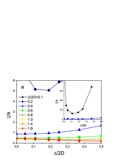
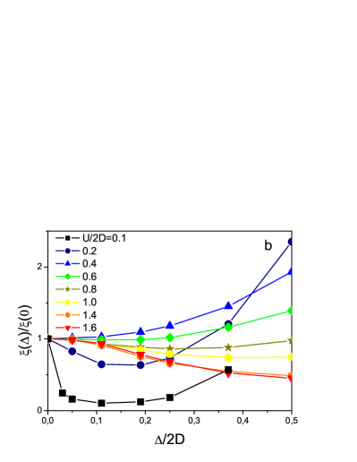
Figure 10: Dependence of coherence length on disorder for different values of Hubbard attraction. (a) — coherence length normalized by lattice parameter $a$. Insert: coherence length dependence on disorder in the limit of weak coupling. (b) — coherence length normalized by its value in the absence of disorder.

In Fig. 10 we show the dependence of coherence length $\xi$ on disorder for different values of coupling. In BCS weak coupling limit and for weak enough disorder we observe the standard “dirty” superconductors dependence $\xi\sim l^{1/2}$, i.e. the coherence length drops with the growth of disorder (cf. insert in Fig. 10(a)). However, for strong enough disorder the coherence length starts to grow with disorder (cf. insert in Fig. 10(a) and Fig. 10(b)), which is mainly related to the noticeable widening of the initial band by disorder and appropriate drop of $U/2D_{eff}$. With further growth of the coupling strength $U/2D\geq 0.4-0.6$ the coherence length $\xi$ becomes of the order of the lattice parameter and is almost independent of disorder. In particular, in strong coupling BEC limit for $U/2D=1.4,1.6$ the growth of disorder to very large values ($\Delta/2D=0.5$) leads to the drop of coherence length by the factor of two (cf. Fig. 10(b)).

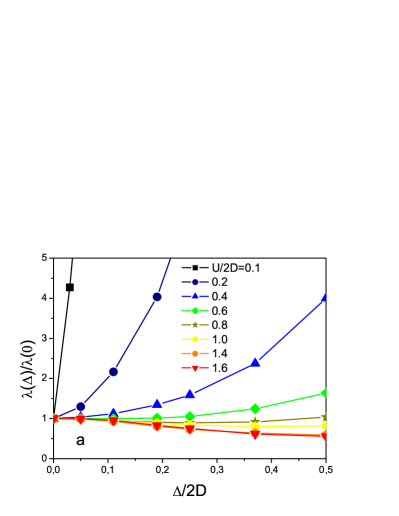
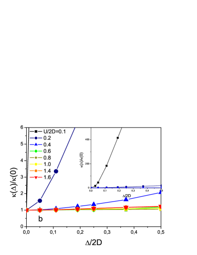
Figure 11: Dependence of penetration depth (a) and Ginzburg – Landau parameter (b) on disorder for different values of Hubbard attraction. Insert: the growth of GL – parameter with disorder in the weak coupling limit.

Dependence of penetration depth on disorder for different values of Hubbard attraction is shown in Fig. 11(a). In the limit of weak coupling in accordance with the theory of “dirty” superconductors disorder leads to the growth of penetration depth $\lambda\sim l^{-1/2}$. With the increase of the coupling strength this growth of penetration depth with disorder slows down and in the limit of very strong coupling $U/2D=1.4,1.6$ penetration depth even slightly diminishes with the growth of disorder. In Fig. 11(b) we show the disorder dependence of dimensionless Ginzburg – Landau parameter $\kappa=\lambda/\xi$. We can see that in the weak coupling limit GL – parameter grows fast with disorder (cf. insert in Fig. 11(b)) in accordance with the theory of “dirty” superconductors, where $\kappa\sim l^{-1}$. With the increase of the coupling the growth of GL – parameter with disorder slows down and in the limit of strong coupling $U/2D>1$ parameter $\kappa$ is practically independent of disorder.

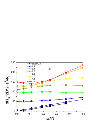
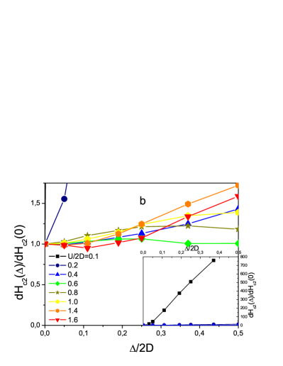
Figure 12: Dependence of the slope of the upper critical field (a) and the slope normalized by its value in the absence of disorder (b) on the level of disorder for different values of Hubbard attraction. Insert: the growth of the slope with disorder in the weak coupling limit.

In Fig. 12 we show the dependence of the slope of the upper critical magnetic field on disorder. In the weak coupling limit we again observe the typical “dirty” superconductor behavior — the slope grows with disorder (cf. Fig. 12(a) and the insert in Fig. 12(b)). For the intermediate coupling region ($U/2D=0.4-0.8$) the slope of the upper critical field is practically independent of disorder. In the limit of very strong coupling at small disorder the slope of the upper critical field can even slightly diminish, but in the limit of strong disorder the slope grows with the growth of disorder scattering.

V Conclusion

In the framework of DMFT+$\Sigma$ generalization of dynamic mean field theory we have studied the effects of disorder on the coefficients of Ginzburg – Landau expansion and the related physical characteristics of superconductors close to $T_{c}$ in attractive Hubbard model. To study the GL – coefficients we have used the combination of DMFT+$\Sigma$ approach and Nozieres – Schmitt-Rink approximation. Calculations were performed for the wide range of the values of attractive potential $U$, from the weak coupling region ($U/2D_{eff}\ll 1$), where instability of the normal phase and superconductivity are well described by BCS model, up to the strong coupling limit ($U/2D_{eff}>1$), where the superconducting transition is related to the Bose – Einstein condensation of compact Cooper pairs.

The growth of the coupling strength $U$ leads to fast drop of all GL – coefficients. Coherence length $\xi$ drops fast with the growth of the coupling strength and for $U/2D\sim 0.4$ becomes of the order of the lattice parameter and only slightly changes with the further growth of the coupling. Penetration depth in “clean” superconductors grows with $U$, while in “dirty” case it drops in the weak coupling region and grows in BEC limit, passing through the minimum in the intermediate (crossover) region of $U/2D\sim 0.4-0.8$. The slope of the upper critical magnetic field grows with $U$. Specific heat discontinuity grows with Hubbard attraction $U$ in the weak coupling region and diminishes in the strong coupling region, passing through the maximum at $U/2D_{eff}\approx 0.55$.

Disorder influence on the critical temperature $T_{c}$, GL – coefficients $A$ and $B$ and specific heat discontinuity is universal — their change is related only to conduction band widening by disorder scattering, i.e. to the replacement $D\to D_{eff}$. Thus, both in BCS – BEC crossover region and in the strong coupling limit both critical temperature and GL – coefficients $A$ and $B$ obey the generalized Anderson theorem — all the influence of disorder reduces to disorder change of the density of states.

GL – coefficient $C$ was studied here in the “ladder” approximation for disorder scattering. Disorder influence upon $C$ is not universal and is not related purely to the conduction band widening by disorder. In the limit of weak coupling $U/2D_{eff}\ll 1$ the behavior of $C$ and the related physical characteristics are well described by the usual theory of “dirty” superconductors. Both $C$ and coherence length drops fast with the growth of disorder, while the penetration depth and the slope of the upper critical magnetic field grow with disorder. In the region of BCS – BEC crossover and in the BEC limit the coefficient $C$ and all physical characteristics are only weakly dependent on disorder. In particular, in BEC limit both the coherence length and penetration depth are only slightly suppressed with the growth of disorder, so that the GL – parameter $\kappa$ is practically independent of disorder.

This work was supported by RSF grant 14-12-00502.

References

- (1) I.M. Lifshitz. Selected works. Physics of Real Crystals and Disordered Systems, “Nauka”, Moscow 1987 (in Russian)
- (2) I.M. Lifshitz. Usp. Fiz. Nauk 83, 617 (1964) [Sov. Phys. - Uspekhi 7, 549 (1964)]
- (3) I.M. Lifshitz. Zh. Eksp. Teor. Fiz. 53, 743 (1967) [Sov. Phys. JETP 26, 462 (1967)]
- (4) A.A. Abrikosov, L.P. Gor’kov. Zh. Eksp. Teor. Fiz. 35, 1558 (1958) [Sov. Phys. JETP 8, 1090 (1959)]
- (5) A.A. Abrikosov, L.P. Gor’kov. Zh. Eksp. Teor. Fiz. 36, 319 (1958) [Sov. Phys. JETP 9, 220 (1959)]
- (6) A.A. Abrikosov, L.P. Gor’kov. Zh. Eksp. Teor. Fiz. 39, 1781 (1960) [Sov. Phys. JETP 12, 1243 (1961)]
- (7) P.W. Anderson. J. Phys. Chem. Solids 11, 26 (1959)
- (8) P.G. De Gennes. Superconductivity of Metals and Alloys. W.A. Benjamin, NY 1966
- (9) M.V. Sadovskii. Physics Reports 282, 225 (1997)
- (10) M.V. Sadovskii. Superconductivity and Localization. World Scientific, Singapore 2000
- (11) L.N. Bulaevskii, S.V. Panyukov, M.V. Sadovskii. Zh. Eksp. Teor. Fiz. 92, 672 (1987) [Sov. Phys. JETP 65, 380 (1987)]
- (12) A. J. Leggett, in “Modern Trends in the Theory of Condensed Matter”, edited by A. Pekalski and J. Przystawa (Springer, Berlin 1980).
- (13) P. Nozieres and S. Schmitt-Rink, J. Low Temp. Phys. 59, 195 (1985)
- (14) Th. Pruschke, M. Jarrell, and J. K. Freericks, Adv. in Phys. 44, 187 (1995).
- (15) A. Georges, G. Kotliar, W. Krauth, and M. J. Rozenberg, Rev. Mod. Phys. 68, 13 (1996).
- (16) D. Vollhardt in “Lectures on the Physics of Strongly Correlated Systems XIV”, eds. A. Avella and F. Mancini, AIP Conference Proceedings vol. 1297, p. 339 (AIP, Melville, New York, 2010); ArXiV: 1004.5069
- (17) M. Keller, W. Metzner, and U. Schollwock. Phys. Rev. Lett. 86, 4612 4615 (2001); ArXiv: cond-mat/0101047
- (18) A. Toschi, P. Barone, M. Capone, and C. Castellani. New Journal of Physics 7, 7 (2005); ArXiv: cond-mat/0411637v1
- (19) J. Bauer, A.C. Hewson, and N. Dupis. Phys. Rev. B 79, 214518 (2009); ArXiv: 0901.1760v2
- (20) A. Koga and P. Werner. Phys. Rev. A 84, 023638 (2011); ArXiv: 1106.4559v1
- (21) N.A. Kuleeva, E.Z. Kuchinskii, M.V. Sadovskii. Zh. Eksp. Teor. Fiz. 146, 304 (2014); [JETP 119, 264 (2014)] ArXiv: 1401.2295
- (22) E.Z.Kuchinskii, I.A.Nekrasov, M.V.Sadovskii. Pisma Zh. Eksp. Teor. Fiz. 82, 217 (2005) [JETP Lett. 82, 198 (2005)]; ArXiv: cond-mat/0506215.
- (23) M.V. Sadovskii, I.A. Nekrasov, E.Z. Kuchinskii, Th. Prushke, V.I. Anisimov. Phys. Rev. B 72, No 15, 155105 (2005); ArXiV: cond-mat/0508585
- (24) E.Z. Kuchinskii, I.A. Nekrasov, M.V. Sadovskii. 32, . 4/5, 528-537 (2006) [Low Temp. Phys. 32, 398 (2006)]; ArXiv: cond-mat/0510376
- (25) E.Z. Kuchinskii, I.A. Nekrasov, M.V. Sadovskii. Usp. Fiz. Nauk 182, 345 (2012) [Physics Uspekhi 55, 325 (2012)]; ArXiv:1109.2305
- (26) E.Z. Kuchinskii, I.A. Nekrasov, M.V. Sadovskii, Zh. Eksp. Teor. Fiz 133, 670 (2008); [JETP 106, 581 (2008)]; ArXiv: 0706.2618.
- (27) E.Z.Kuchinskii, N.A.Kuleeva, I.A.Nekrasov, M.V.Sadovskii. Zh. Eksp. Teor. Fiz. 137, 368 (2010); [JETP 110, 325 (2010)]; ArXiv: 0908.3747
- (28) E.Z.Kuchinskii, I.A.Nekrasov, M.V.Sadovskii. Phys. Rev. B 80, 115124 (2009); ArXiv: 0906.3865
- (29) E.Z. Kuchinskii, I.A. Nekrasov, M.V. Sadovskii. Phys. Rev. B 75, 115102-115112 (2007); ArXiv: cond-mat/0609404.
- (30) E.Z. Kuchinskii, N.A. Kuleeva, M.V. Sadovskii. Pisma Zh. Eksp. Teor. Fiz. 100, 213 (2014) [JETP Letters 100, 192 (2014)]; ArXiv: 1406.5603
- (31) E.Z. Kuchinskii, N.A. Kuleeva, M.V. Sadovskii. Zh. Eksp. Teor. Fiz. 147, 1220 (2015) [JETP 120, 1095 (2015)]; ArXiv:1411.1547
- (32) E.Z. Kuchinskii, M.V. Sadovskii. Zh. Eksp. Teor. Fiz. 149, 589 (2016) [JETP 122, 510 (2016)]; ArXiv:1507.07654
- (33) R. Micnas. Acta Physica Polonica A100(s), 177 (2001); ArXiv: cond-mat/0211561v2
- (34) M. Drechsler and W. Zwerger. Ann. Phys.(Leipzig) 1, 15 (1992)
- (35) S. Stintzing and W. Zwerger. Phys. Rev. B 56, 9004 (1997); ArXiv: cond-mat/9703129v2
- (36) E.Z. Kuchinskii, N.A. Kuleeva, M.V. Sadovskii. Zh. Eksp. Teor. Fiz. 149, 430 438 (2016) [JETP 122, 375 (2016)]; ArXiv:1507.07649
- (37) M.V. Sadovskii. Diagrammatics. World Scientific, Singapore 2006
- (38) R. Bulla, T.A. Costi, T. Pruschke, Rev. Mod. Phys. 60, 395 (2008).