Swift follow-up of gravitational wave triggers: results from the first aLIGO run and optimisation for the future

Abstract

During its first observing run, in late 2015, the advanced LIGO facility announced 3 gravitational wave (GW) triggers to electromagnetic follow-up partners. Two of these have since been confirmed as being of astrophysical origin: both are binary black hole mergers at $\sim\,$500 Mpc; the other trigger was later found not to be astrophysical. In this paper we report on the Swift follow up observations of the second and third triggers, including details of 21 X-ray sources detected; none of which can be associated with the GW event. We also consider the challenges that the next GW observing run will bring as the sensitivity and hence typical distance of GW events will increase. We discuss how to effectively use galaxy catalogues to prioritise areas for follow up, especially in the presence of distance estimates from the GW data. We also consider two galaxy catalogues and suggest that the high completeness at larger distances of the 2MASS Photometric Redshift Catalogue (2MPZ) makes it very well suited to optimise Swift follow-up observations.

1 Introduction

In the last quarter of 2015, the Advanced Laser Interferometer Gravitational-wave Observatory observatory (aLIGO; LIGO Scientific Collaboration et al. 2015; Abbott et al. 2016f) performed its first observing run (‘O1’) searching for gravitational waves (GW). Each potential GW event was assigned a false alarm rate (FAR) indicating the frequency with which a noise event with a signal of the observed strength is expected to arise. Partner electromagnetic (EM) facilities, including Swift (Gehrels et al., 2004), were notified of GW signals with an FAR of less than one per month (Abbott et al., 2016a). O1 yielded the detection of two GW events, which have been confidently identified as binary black hole (BBH) mergers: GW150914 (Abbott et al., 2016d) and GW151226 (Abbott et al., 2016e), and there was a further trigger (G194575) from the online analysis which was later determined to be a noise event. Another possible merger event was detected in offline analysis of the O1 data [LVT151012; (The LIGO Scientific Collaboration et al., 2016)]. Details of that event were not provided to EM partners until 2016 April, so no Swift follow up was performed. The full results of O1 were reported by Abbott et al. (2016b).

Whilst the direct detection of GW was a significant achievement which marked the beginning of a new era of astronomy, in order to maximise the scientific potential of such discoveries, complementary EM data are needed. The three events reported so far are all believed to be stellar-mass BBH mergers, which were not expected to produce significant EM emission (e.g. Kamble & Kaplan, 2013). However, Fermi-GBM reported a possible low-significance event 0.4 s after the GW trigger for GW150914, which may be associated with the GW event (Connaughton et al., 2016). In the days following the announcement of this, many authors suggested that EM emission from stellar-mass BBH is possible given the correct binary parameters, or a charged black hole (e.g. Zhang, 2016; Yamazaki et al., 2016; Perna et al., 2016; Loeb, 2016), although others suggested that a physical association between the GW and GBM events was unlikely (Lyutikov, 2016). Further, INTEGRAL reported no detection (Savchenko et al., 2016) and suggest that this casts doubt over whether the object detected by GBM was astrophysical in origin. This issue will likely only be resolved by future GW detections of BBH with both contemporaneous and follow-up EM observations.

Regardless of whether BBH mergers give rise to EM emission, aLIGO is also expected to detect GW from the coalescence of binary neutron star systems or neutron star-black hole systems. These are both expected to produce multi-wavelength EM radiation, for example in the form of a short gamma-ray burst (sGRB, e.g. Berger 2014) if the binary is viewed close to face-on, or a kilonova (Li & Paczyński, 1998) regardless of the jet orientation; see e.g. Nakar & Piran (2011); Metzger & Berger (2012); Zhang (2013) for a discussion of possible EM counterparts to such events.

In an earlier paper (Evans et al. 2016b; hereafter ‘paper I’) we presented the Swift observations of GW150914. In this work we present the results of the Swift observations of the other two triggers reported to the EM teams during O1, and consider how the Swift follow-up strategy may best evolve for the second run (O2) expected in the second half of 2016.

Throughout this paper, all errors are given at the 1-$\sigma$ level, unless stated otherwise.

2 Swift observations

The Swift satellite (Gehrels et al., 2004) contains three complementary instruments. The Burst Alert Telescope (BAT; Barthelmy et al. 2005) is a 15–350 keV coded-mask instrument with a field of view $\sim\,$2 sr. Its primary role is to trigger on new transient events such as GRBs. The other two instruments are narrow-field instruments, used for example to follow up GRBs detected by BAT. The X-ray telescope (XRT; Burrows et al. 2005) is a 0.3–10 keV focusing instrument with a peak effective area of 110 cm² at 1.5 keV and a roughly circular field of view with radius 12.3^′. The ultra-violet/optical telescope (UVOT; Roming et al. 2005) has 6 optical filters covering 1600–6240 Å and a white filter covering 1600–8000 Å), with a peak effective area of 50 cm² in the $u$ band. The field of view is square, $\sim\,$17^′ to a side.

The ideal scenario for Swift to observe a GW event would be for BAT to detect EM emission (e.g. an sGRB) independently of the GW trigger on the same event. Swift would then automatically slew and gather prompt XRT and UVOT data. An sGRB is only seen if the coalescing binary is inclined such that the jet is oriented towards Earth; the opening angles of sGRB jets are not well known, however the observational limits are in the range $\sim\,$5–25^∘(Burrows et al., 2006; Grupe et al., 2006; Fong et al., 2015; Zhang et al., 2015; Troja et al., 2016), therefore from purely geometrical constraints, we expect only a minority of binary neutron star/neutron star-black hole mergers detected in GW to be accompanied by an sGRB (e.g. for a jet angle of 10^∘, only 1.5% will be viewed on-axis), whereas the GW signal is only modestly affeted by binary inclination. Some authors (e.g. Troja et al. 2010; Tsang 2013) have suggested that the neutron star crust can be disrupted prior to the merger and that this could give rise to an isotropic precursor, i.e. BAT could in principle detect such emission from an off-axis GRB. However, these could well be too faint to trigger Swift-BAT. Also, while an excellent GRB-detection machine, Swift-BAT can only observe $\sim\,$1/6 of the sky at any given time. The combination of these factors means that, while a simultaneous ALIGO-BAT detection would be scientifically optimal, it is not a particularly likely occurrance.

In addition, Swift can respond to the GW trigger, and observe a portion of the GW error region (which typically hundreds of square degrees in size) rapidly with its narrow-field telescopes. Evans et al. (2016a) discussed optimal ways to do this, focusing primarily on the XRT, since it has a larger field of view than the UVOT, and the expected rate of unrelated transient events in the X-ray range, while not well constrained, is expected to be lower than in the optical bands (see Kanner et al. 2013; Evans et al. 2016a for a discussion of X-ray transient rates). Their suggested approach was to modify the GW error region by means of a galaxy catalogue (they used the Gravitational Wave Galaxy Catalogue (GWGC): White et al. 2011), weighting each pixel in the GW skymap by the luminosity of the catalogued galaxies in that pixel, and then to observe in a succession of short observations, in decreasing order of probability in this combined map. A more detailed Bayesian approach to this was discussed by Fan et al. (2014). As we reported in paper I, the ability to observe a large number of fields with short exposures required operational changes for Swift which were not completed in time for O1, therefore we were only able to observe a relatively small part of the GW error regions for the triggers during that run. As described in paper I for GW150914, we combined the GW error region for each trigger in O1 with GWGC, weighting the galaxies according to their $B$-band luminosities, and selecting XRT fields based on the resultant probability map.

The data analysis approach was described in paper I so here we offer only a précis. For XRT, the source detection system was based on that of Evans et al. (2014), slightly modified to support shorter exposures. Every source detected was automatically assigned a Rank of 1–4 describing how likely it was to be the counterpart to the GW event, with 1 being the most likely. This was based on whether the source was previously catalogued, its flux compared to previous detection or upper limits and its proximity to a known galaxy (full definitions of the ranks are in paper I). The detection system also produces warning flags for sources which it believes may be spurious due to effects, such as diffuse X-ray emission (the detection system is designed for point sources), or instrumental artefacts, such as stray light or optical loading (see Evans et al. 2014 section 3.4 and fig. 5). For each source detected, a GCN ‘Counterpart’ notice was automatically produced as soon as the source was detected; this contained standard details (position, time of detection, flux) and also the rank and any warning flags. All sources were checked by humans, and any which were spurious were removed, and the verified sources reported in LVC/GCN circulars (Evans et al. 2015a, b, c, f, g, h, i, j).

UVOT data were analysed using standard heasoft tools, and an automated pipeline was used to search for transients. Visual screening was applied to UVOT images, using the Digitized Sky Survey as a comparison. Although no rank 1 or 2 X-ray sources were found during O1, the UVOT data around any such sources would also have been closely inspected by eye.

2.1 GW150914

GW150914 was detected at the end of the aLIGO engineering run immediately prior to O1, and was the first ever direct detection of GW. The Swift results for this event were reported in full in paper I. Recently (2016 April) we reobserved the GW error region of GW150914, as the final step to commission the ability to perform large-scale rapid tiling with Swift. Swift observed 426 fields during the UT day 2016 April 21 with 60 s of exposure per field, covering a total of 53 sq deg. Only one X-ray source was detected in these observations, the known X-ray emitter 1RXS J082709.9$-$650447, which was detected with a flux consistent with that from the Rosat observations (Voges et al., 1999). The scientific ‘result’ from these observations is that, as expected, the only background X-ray source found was a known (rank 4) object; therefore we are optimistic that a transient should be easy to distinguish. However, these observations also demonstrate that Swift is now capable of performing large-scale tiling in response to a GW trigger.

2.2 Trigger G194575

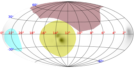
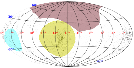
Figure 1: The ‘BAYESTAR’ GW localisation map for trigger G194575, produced by the LVC team on 2015 October 22 (top), combined with our luminosity-weighted GWGC map (bottom). Coordinates are equatorial, J2000. The yellow and cyan circles indicate the regions towards which XRT and UVOT cannot point due to proximity to the Sun and Moon respectively. The large maroon area is the BAT partially coded field of view at the time of the GW event. For this event, unfortunately the majority of the error region was unobservable due to its proximity to the Sun.

Table 1: Swift observations of the error region of LVC trigger G194575

Pointing direction	Start timea	Exposure	Source	XRT limit	UVOT magnitude
(J2000)	(UTC)	(s)		0.3–10 keV
				erg cm-2 s-1
$00^{h}11^{m}27.60^{s},-06^{\circ}25^{\prime}38.3^{\prime\prime}$	Oct 27 01:17:46	1985	LSQ15bjb	1.4$\times 10^{-13}$	$u$=16.7
$00^{h}58^{m}13.27^{s},-03^{\circ}39^{\prime}50.4^{\prime\prime}$	Nov 06 23:22:15	9948b	iPTF15dld	4.9$\times 10^{-14}$	N/Ac

^a All observations were in 2015.
^b The observation of iPTF15dld was not a continuous exposure due to Swift’s low-Earth orbit. The 10 ks of data were obtained between the Nov 6 at 23:22:15 and Nov 07 at 10:16:44 UT.
^c The source could not be deconvolved from the host galaxy in the UVOT data, so no magnitude was derived.

The aLIGO ‘compact binary coalescence’ (CBC) pipeline, which uses a template library of expected GW waveforms from merging compact binaries, triggered on 2015 October 22 at 13:33:19.942 UT. The detected signal had an FAR of 9.65$\times 10^{-8}$ Hz, equivalent to one per four months (Singer et al., 2015a). Unfortunately, most of the higher probability areas of the error region were too close to the Sun for observations with Swift (Fig. 1), therefore only the low probability regions were observable. Additionally, offline analysis of the GW signal reduced the FAR to 8.19$\times 10^{-6}$ Hz (one per 1.41 days), and it was therefore determined not to be a real GW event (LIGO Scientific Collaboration, 2015a). Although this trigger is therefore not of astrophysical significance, one point of procedural interest for future triggers is worth noting. Before the significance of the trigger had been downgraded, two sources identified by ground-based observatories were reported as being of potential interest: LSQ15bjb (Rabinowitz et al., 2015a) and iPTF15dld (Singer et al., 2015b), which were detected by the La Silla QUEST and iPTF ground-based facilities respectively. Swift observed both of these sources and, finding no X-ray counterpart, we reported upper limits (Evans et al., 2015d, e). LSQ15bjb was originally reported as an uncatalogued and rapidly brightening optical source (Rabinowitz et al., 2015a), which was subsequently classified as a type Ia supernova (Piranomonte et al., 2015). iPTF15dld was one of several optical transients reported by (Singer et al., 2015b) that were consistent in position with a known galaxy at $z<0.1$; it later transpired that this source had been detected by by La Silla QUEST 19 days before the GW event (Rabinowitz et al., 2015b).

Details of the Swift observations and results for these two sources are given in Table 1. This demonstrates the ability to be flexible when performing Swift GW follow up, and perform targetted observation of point sources detected by other facilities, as well the blind searches.

2.3 GW 151226

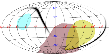
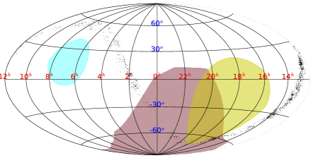
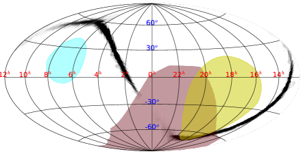
Figure 2: The ‘BAYESTAR’ GW localisation map of GW151226, produced by the LVC team on 2015 December 26 (top), combined with our luminosity-weighted GWGC map (middle). The bottom panel is the refined ‘LALInference‘ map. The yellow and cyan circles are as in Fig. 1. These images are centred on RA=0, unlike Fig. 1, so that the regions are more visible.

Table 2: Swift observations of the error region of GW 151226.

Pointing direction	Start timea	Exposure
(J2000)	(UTC)	(s)
$09^{h}43^{m}50.88^{s},+59^{\circ}48^{\prime}02.9^{\prime\prime}$	Dec 27 at 18:37:03	1384
$13^{h}30^{m}7.20^{s},-21^{\circ}13^{\prime}01.2^{\prime\prime}$	Dec 27 at 20:19:11	333
$13^{h}31^{m}33.84^{s},-21^{\circ}13^{\prime}01.2^{\prime\prime}$	Dec 27 at 20:21:31	325
$13^{h}30^{m}50.64^{s},-21^{\circ}30^{\prime}32.4^{\prime\prime}$	Dec 27 at 20:23:53	288
$13^{h}29^{m}23.76^{s},-21^{\circ}30^{\prime}32.4^{\prime\prime}$	Dec 27 at 20:26:14	318
$13^{h}28^{m}40.56^{s},-21^{\circ}13^{\prime}01.2^{\prime\prime}$	Dec 27 at 20:28:34	305
$13^{h}29^{m}23.76^{s},-20^{\circ}55^{\prime}30.0^{\prime\prime}$	Dec 27 at 20:30:53	313
$13^{h}30^{m}50.64^{s},-20^{\circ}55^{\prime}30.0^{\prime\prime}$	Dec 27 at 20:33:13	340
$13^{h}32^{m}17.28^{s},-20^{\circ}55^{\prime}30.0^{\prime\prime}$	Dec 27 at 20:35:30	213
$13^{h}33^{m}0.48^{s},-21^{\circ}13^{\prime}01.2^{\prime\prime}$	Dec 27 at 20:37:49	285
$13^{h}32^{m}17.28^{s},-21^{\circ}30^{\prime}32.4^{\prime\prime}$	Dec 27 at 20:40:07	310
$13^{h}31^{m}33.84^{s},-21^{\circ}48^{\prime}00.0^{\prime\prime}$	Dec 27 at 20:42:25	325
$13^{h}30^{m}7.20^{s},-21^{\circ}48^{\prime}00.0^{\prime\prime}$	Dec 27 at 20:44:42	378
$13^{h}28^{m}40.56^{s},-21^{\circ}48^{\prime}00.0^{\prime\prime}$	Dec 27 at 20:46:59	318
$13^{h}27^{m}57.12^{s},-21^{\circ}30^{\prime}32.4^{\prime\prime}$	Dec 27 at 20:49:11	320
$13^{h}27^{m}13.68^{s},-21^{\circ}13^{\prime}01.2^{\prime\prime}$	Dec 27 at 20:51:23	323
$13^{h}27^{m}57.12^{s},-20^{\circ}55^{\prime}30.0^{\prime\prime}$	Dec 27 at 20:53:32	320
$13^{h}28^{m}40.56^{s},-20^{\circ}38^{\prime}02.4^{\prime\prime}$	Dec 27 at 20:55:39	308
$13^{h}30^{m}7.20^{s},-20^{\circ}38^{\prime}02.4^{\prime\prime}$	Dec 27 at 20:57:44	323
$13^{h}31^{m}33.84^{s},-20^{\circ}38^{\prime}02.4^{\prime\prime}$	Dec 27 at 20:59:47	290
$13^{h}49^{m}32.88^{s},-30^{\circ}29^{\prime}16.8^{\prime\prime}$	Dec 28 at 01:14:23	308
$13^{h}51^{m}6.72^{s},-30^{\circ}29^{\prime}16.8^{\prime\prime}$	Dec 28 at 01:16:22	193
$13^{h}50^{m}19.92^{s},-30^{\circ}46^{\prime}48.0^{\prime\prime}$	Dec 28 at 01:18:21	157
$13^{h}48^{m}46.08^{s},-30^{\circ}46^{\prime}48.0^{\prime\prime}$	Dec 28 at 01:20:21	295
$13^{h}47^{m}59.04^{s},-30^{\circ}29^{\prime}16.8^{\prime\prime}$	Dec 28 at 01:22:19	310
$13^{h}48^{m}46.08^{s},-30^{\circ}11^{\prime}49.2^{\prime\prime}$	Dec 28 at 01:24:16	438
$13^{h}50^{m}19.92^{s},-30^{\circ}11^{\prime}49.2^{\prime\prime}$	Dec 28 at 01:26:12	300
$13^{h}51^{m}53.76^{s},-30^{\circ}11^{\prime}49.2^{\prime\prime}$	Dec 28 at 01:28:08	310
$13^{h}52^{m}40.56^{s},-30^{\circ}29^{\prime}16.8^{\prime\prime}$	Dec 28 at 01:30:04	423
$13^{h}51^{m}53.76^{s},-30^{\circ}46^{\prime}48.0^{\prime\prime}$	Dec 28 at 01:32:00	165
$13^{h}51^{m}6.72^{s},-31^{\circ}04^{\prime}19.2^{\prime\prime}$	Dec 28 at 01:33:55	290
$13^{h}49^{m}32.88^{s},-31^{\circ}04^{\prime}19.2^{\prime\prime}$	Dec 28 at 01:35:49	305
$13^{h}47^{m}59.04^{s},-31^{\circ}04^{\prime}19.2^{\prime\prime}$	Dec 28 at 01:37:42	313
$13^{h}47^{m}12.24^{s},-30^{\circ}46^{\prime}48.0^{\prime\prime}$	Dec 28 at 01:39:33	418
$13^{h}46^{m}25.44^{s},-30^{\circ}29^{\prime}16.8^{\prime\prime}$	Dec 28 at 01:41:22	245
$13^{h}47^{m}12.24^{s},-30^{\circ}11^{\prime}49.2^{\prime\prime}$	Dec 28 at 01:43:08	368
$13^{h}47^{m}59.04^{s},-29^{\circ}54^{\prime}18.0^{\prime\prime}$	Dec 28 at 01:44:53	303
$13^{h}49^{m}32.88^{s},-29^{\circ}54^{\prime}18.0^{\prime\prime}$	Dec 28 at 01:46:37	165
$13^{h}51^{m}6.72^{s},-29^{\circ}54^{\prime}18.0^{\prime\prime}$	Dec 28 at 01:48:19	127
$14^{h}03^{m}9.12^{s},-34^{\circ}09^{\prime}25.2^{\prime\prime}$	Dec 28 at 09:14:07	80
$14^{h}04^{m}47.04^{s},-34^{\circ}09^{\prime}25.2^{\prime\prime}$	Dec 28 at 09:16:09	215
$14^{h}03^{m}58.08^{s},-34^{\circ}26^{\prime}52.8^{\prime\prime}$	Dec 28 at 09:18:05	315
$14^{h}02^{m}20.40^{s},-34^{\circ}26^{\prime}52.8^{\prime\prime}$	Dec 28 at 09:20:03	218
$14^{h}01^{m}31.68^{s},-34^{\circ}09^{\prime}25.2^{\prime\prime}$	Dec 28 at 09:21:59	87
$14^{h}02^{m}20.40^{s},-33^{\circ}51^{\prime}54.0^{\prime\prime}$	Dec 28 at 09:23:54	115
$14^{h}03^{m}58.08^{s},-33^{\circ}51^{\prime}54.0^{\prime\prime}$	Dec 28 at 09:25:49	90
$14^{h}05^{m}35.76^{s},-33^{\circ}51^{\prime}54.0^{\prime\prime}$	Dec 28 at 09:27:42	105
$14^{h}06^{m}24.48^{s},-34^{\circ}09^{\prime}25.2^{\prime\prime}$	Dec 28 at 09:29:37	100
$14^{h}05^{m}35.76^{s},-34^{\circ}26^{\prime}52.8^{\prime\prime}$	Dec 28 at 09:31:31	92
$14^{h}04^{m}47.04^{s},-34^{\circ}44^{\prime}24.0^{\prime\prime}$	Dec 28 at 09:33:25	107
$14^{h}01^{m}31.68^{s},-34^{\circ}44^{\prime}24.0^{\prime\prime}$	Dec 28 at 09:37:08	285
$14^{h}00^{m}42.72^{s},-34^{\circ}26^{\prime}52.8^{\prime\prime}$	Dec 28 at 09:38:57	135
$13^{h}59^{m}54.00^{s},-34^{\circ}09^{\prime}25.2^{\prime\prime}$	Dec 28 at 09:40:44	295

^a Observations were 2015 December or 2016 January.

Table 3: continued

Pointing direction	Start timea	Exposure
(J2000)	(UTC)	(s)
$14^{h}00^{m}42.72^{s},-33^{\circ}51^{\prime}54.0^{\prime\prime}$	Dec 28 at 09:42:31	310
$14^{h}01^{m}31.68^{s},-33^{\circ}34^{\prime}22.8^{\prime\prime}$	Dec 28 at 09:44:13	195
$14^{h}03^{m}9.12^{s},-33^{\circ}34^{\prime}22.8^{\prime\prime}$	Dec 28 at 09:45:56	401
$14^{h}04^{m}47.04^{s},-33^{\circ}34^{\prime}22.8^{\prime\prime}$	Dec 28 at 09:47:37	278
$12^{h}31^{m}7.44^{s},+12^{\circ}18^{\prime}50.4^{\prime\prime}$	Dec 28 at 15:24:31	443
$12^{h}32^{m}30.24^{s},+12^{\circ}18^{\prime}50.4^{\prime\prime}$	Dec 28 at 15:26:54	406
$12^{h}31^{m}48.96^{s},+12^{\circ}01^{\prime}22.8^{\prime\prime}$	Dec 28 at 15:29:21	438
$12^{h}30^{m}26.16^{s},+12^{\circ}01^{\prime}22.8^{\prime\prime}$	Dec 28 at 15:31:47	431
$12^{h}29^{m}44.88^{s},+12^{\circ}18^{\prime}50.4^{\prime\prime}$	Dec 28 at 15:34:11	423
$12^{h}30^{m}26.16^{s},+12^{\circ}36^{\prime}21.6^{\prime\prime}$	Dec 28 at 15:36:36	386
$12^{h}31^{m}48.96^{s},+12^{\circ}36^{\prime}21.6^{\prime\prime}$	Dec 28 at 15:38:53	418
$12^{h}33^{m}11.52^{s},+12^{\circ}36^{\prime}21.6^{\prime\prime}$	Dec 28 at 15:41:09	416
$12^{h}33^{m}53.04^{s},+12^{\circ}18^{\prime}50.4^{\prime\prime}$	Dec 28 at 15:43:22	423
$12^{h}33^{m}11.52^{s},+12^{\circ}01^{\prime}22.8^{\prime\prime}$	Dec 28 at 15:45:34	413
$12^{h}32^{m}30.24^{s},+11^{\circ}43^{\prime}51.6^{\prime\prime}$	Dec 28 at 15:47:47	421
$12^{h}31^{m}7.44^{s},+11^{\circ}43^{\prime}51.6^{\prime\prime}$	Dec 28 at 15:49:58	433
$12^{h}29^{m}44.88^{s},+11^{\circ}43^{\prime}51.6^{\prime\prime}$	Dec 28 at 15:52:08	411
$12^{h}29^{m}3.12^{s},+12^{\circ}01^{\prime}14.7^{\prime\prime}$	Dec 28 at 15:54:15	423
$12^{h}28^{m}22.08^{s},+12^{\circ}18^{\prime}50.4^{\prime\prime}$	Dec 28 at 15:56:21	418
$12^{h}29^{m}3.36^{s},+12^{\circ}36^{\prime}21.6^{\prime\prime}$	Dec 28 at 15:58:23	428
$12^{h}29^{m}44.88^{s},+12^{\circ}53^{\prime}52.8^{\prime\prime}$	Dec 28 at 16:00:24	335
$12^{h}31^{m}7.44^{s},+12^{\circ}53^{\prime}52.8^{\prime\prime}$	Dec 28 at 16:02:46	263
$12^{h}32^{m}30.24^{s},+12^{\circ}53^{\prime}52.8^{\prime\prime}$	Dec 28 at 16:05:01	328
$02^{h}59^{m}41.20^{s},+25^{\circ}14^{\prime}12.2^{\prime\prime}$	Jan 05 at 17:43:10	3763b
$02^{h}32^{m}59.75^{s},+18^{\circ}38^{\prime}07.0^{\prime\prime}$	Jan 07 at 15:52:50	17182c

^a Observations were 2015 December or 2016 January.
^b Observations of PS15dqa. These observations were not continuous but occurred in two ‘snapshots’ on consecutive Swift orbits.
^c Observations of PS15dpn. This was observed every few days for two weeks, the last observation occurring on 2016 January 25.

Table 4: XRT sources detected in observations of GW151226

Position	Errora	Flux (erg cm-2 s-1)	Rank	Catalogued match	Separation
(J2000)	(arcsec)	0.3–10 keV			(arcsec)
$13^{h}30^{m}13.26^{s},-20^{\circ}54^{\prime}16.4^{\prime\prime}$	5.3	$(4.1\pm 2.2)\times 10^{13}$	3
$12^{h}30^{m}47.32^{s},+12^{\circ}20^{\prime}20.3^{\prime\prime}$	6.6	$(6.3\pm 2.3)\times 10^{12}$	3
$12^{h}32^{m}7.03^{s},+11^{\circ}51^{\prime}21.6^{\prime\prime}$	6.6	$(6.7\pm 2.6)\times 10^{13}$	3
$13^{h}30^{m}16.30^{s},-20^{\circ}55^{\prime}26.1^{\prime\prime}$	6.0	$(4.6\pm 2.8)\times 10^{13}$	3
$12^{h}31^{m}29.59^{s},+11^{\circ}52^{\prime}37.8^{\prime\prime}$	6.7	$(6.0\pm 2.7)\times 10^{13}$	3
$12^{h}31^{m}42.62^{s},+12^{\circ}19^{\prime}45.3^{\prime\prime}$	13.1	$(7.7\pm 4.4)\times 10^{13}$	3
$13^{h}29^{m}25.00^{s},-21^{\circ}13^{\prime}37.2^{\prime\prime}$	5.7	$(1.1\pm 0.4)\times 10^{12}$	3
$02^{h}59^{m}42.18^{s},+25^{\circ}12^{\prime}46.5^{\prime\prime}$	5.8	$(6.3\pm 3.4)\times 10^{14}$	3
$12^{h}30^{m}59.30^{s},+12^{\circ}11^{\prime}33.9^{\prime\prime}$	5.6	$(8.3\pm 4.6)\times 10^{13}$	4	3XMM J123059.4+121131	2.7
$13^{h}49^{m}19.27^{s},-30^{\circ}18^{\prime}35.4^{\prime\prime}$	4.1	$(5.3\pm 1.2)\times 10^{11}$	4	1SXPS J134919.2-301834	6.5
$13^{h}48^{m}44.40^{s},-30^{\circ}29^{\prime}46.5^{\prime\prime}$	5.9	$(2.2\pm 0.5)\times 10^{12}$	4	XMMSL1 J134844.6-302948	2.7
$13^{h}30^{m}7.66^{s},-20^{\circ}56^{\prime}11.1^{\prime\prime}$	6.0	$(8.5\pm 3.1)\times 10^{13}$	4	1SXPS J133007.7-205619	8.4
				[RKV2003] QSO J1330-2056 abs 0.84992	5.3b
$12^{h}30^{m}42.99^{s},+12^{\circ}23^{\prime}17.1^{\prime\prime}$	5.5	$(1.8\pm 0.5)\times 10^{10}$	4	2RXP J123044.7+122331	28.9
				[SFH81] 1157	7.9b
$13^{h}30^{m}7.02^{s},-21^{\circ}41^{\prime}59.8^{\prime\prime}$	5.1	$(2.7\pm 0.6)\times 10^{12}$	4	1RXS J133006.8-214156	3.9
				[RKV2003] QSO J1330-2142 abs 0.3014	2.9b
$13^{h}49^{m}4.00^{s},-30^{\circ}17^{\prime}46.3^{\prime\prime}$	7.6	$(2.0\pm 0.5)\times 10^{12}$	4	XMMSL1 J134904.4-301745	3.6
				[RP98d] P6	6.3b
$12^{h}31^{m}12.74^{s},+12^{\circ}03^{\prime}17.1^{\prime\prime}$	7.3	$(3.0\pm 1.1)\times 10^{13}$	4	3XMM J123113.1+120307	6.6
				2MASX J12311311+1203075	6.6b

^a 90% confidence
^b From SIMBAD

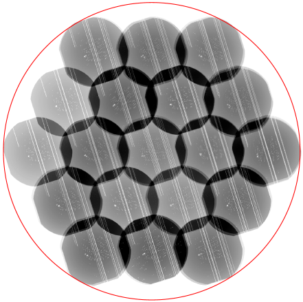
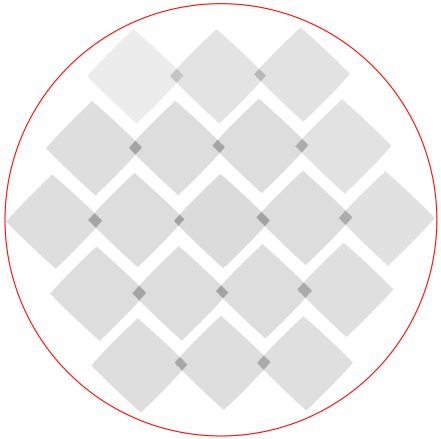
Figure 3: An example XRT (top) and UVOT (bottom) exposure map from a 19-point tile used in the follow-up observations of GW151226. The circle is shown for scale and has radius 0.88^∘.

The CBC pipeline triggered on 2015 December 26 at 03:38:53.648 UT, with a signal with FAR lower than one per month (LIGO Scientific Collaboration, 2015b); this was later refined to an FAR lower than one per hundred years (LIGO Scientific Collaboration, 2015c). The GW waveform indicated that this was a high-mass event, most likely a BH-BH merger (LIGO Scientific Collaboration, 2015b). As with both previous triggers, a portion of the error region was too close to the Sun to observe with Swift (Fig. 2). The trigger was announced to the follow-up community on 2015 December 27 at 16:28 UT, and Swift observations began at 18:35 UT on the same day. We followed the same procedure as for the earlier triggers, selecting the most probable XRT fields after combining with the GWGC galaxy catalogue. However, after the first field had been observed, we modified this approach and instead of selecting single XRT fields, we selected regions covered by a set of 19 tiled pointings (Fig. 3). We uploaded four such observation sets, as detailed in Table 2. We also performed additional sets of observations, observing the locations of PS15dqa and PS15dpn (Chambers et al., 2015): optical sources highlighted as potentially interesting. PS15dpn was observed repeatedly for several days in order to track the UV evolution of its light curve. This source is not believed to be related to the GW trigger, and the PS15dpn data are not presented in this work.

The GW localisation of GW151226 is shown in Fig. 2. At the time of the Swift observations, only the ‘BAYESTAR’ map (produced by the low-latency pipeline; Singer & Price 2016) was available (top two panels). A revised skymap produced by the offline ‘LALInference’ pipeline [Veitch et al. (2015); bottom panel of Fig. 2] was made available on 2016 January 16 (LIGO Scientific Collaboration & VIRGO, 2015), well after our observations had been completed. The BAT field of view overlaps the GW localisations, covering 14% of the probability in the ‘BAYESTAR’ map and 15% from the revised map [these probabilities are higher, $\sim\,$29%  and 33% after weighting by the GWGC, however since the distance to this merger is large ($440^{+180}_{-190}$ Mpc; Abbott et al. 2016e) and GWGC only contains galaxies to 100 Mpc, the galaxy-weighted map is not appropriate]. We created a 15–350 keV BAT light curve from $T_{0}-100$ to $T_{0}+100$ s ($T_{0}$ is the GW trigger time) with bins of 1.024 s. No signal is seen, at the 4-$\sigma$ level with an upper limit (also 4 $\sigma$) of 303.6 counts in a single bin. We used 4 $\sigma$ as the limit rather than 3 $\sigma$ because, for a 1.024-s binned light curve we expect a 3-$\sigma$ noise fluctuation every $\sim\,$6 minutes, therefore the chance of a spurious signal in our data is high. At 4 $\sigma$ noise fluctuations are expected only every 4.4 hours. To convert this to a flux limit we assumed a typical short GRB BAT spectrum: a power-law with a photon index of 1.32. The counts-to-flux conversion depends on the angle of the source to the BAT boresight which, since the source position is poorly contsrained, is not known. If the GW source was close to the BAT boresight (‘fully coded’ by the BAT mask) the upper limit is 4.3$\times 10^{-8}$ erg

$$cm^{-2}\ s^{-1}.Forasourcewhichishalfcodedbythemask(45^{\circ}\ offaxis)thelimitis1.7\times 10^{-7}ergcm^{-2}\ s^{-1},andifthesourcewasonly10\%\ codedbytheBATmask(56^{\circ}\ offaxis)thelimitis9.0\times 10^{-7}ergcm^{-2}\ s^{-1}.\par TheinitialXRTobservations(i.e.notincludingtheobservationsofPS15dqaorPS15dpn)covered8.5squaredegreesandenclosed0.9\%\ oftheprobabilityinboththeoriginalandrevisedskymaps.55sourcesweredetectedintheseobservations,however39ofthesewereartefactsofanareaofextendedemission(allbut2ofwhichwerecorrectlyflaggedassuchbytheautomatedsystemandinthecounterpartnotices,thefinaltwowereremovedbyvisualinspection).Detailsofthe16genuinesources,noneofwhichisbelievedtobethecounterpart,aregiveninTable~{}\ref{tab:res_151226};eightofthesewererank3sources(uncatalogued,butbelowpreviouscataloguedetectionlimits),andeightrank4(cataloguedsourcesatfluxesconsistentwiththeircataloguedvalues).\par NouncataloguedsourceswerefoundintheUVOTdata.\par$$

2.3.1 Late observations

On 2016 January 13 we performed a new set of observations of the error region of GW151226. This consisted of 201 short ($\sim\,60$ s) exposures, and was primarily performed as part of commissioning the ability to rapidly tile GW error regions with Swift. These observations precede those reported in Section 2.1 (i.e. the 2016 April observations of GW150914), and the test was only allowed to run for a few hours. This test revealed a bug in our software affecting low resolution GW localisations (healpix-format maps with nside$<512$), as a result of which the 201 fields selected did not lie within the GW error region (this bug is now fixed).

As with the 2016 April 24-hour test (Section 2.1), the only X-ray sources found were two rank 4 sources. Fortuitously, these both lay in an area of the sky previously observed by Swift-XRT, and the two sources were in the 1SXPS catalogue (Evans et al., 2014), which allows us to compare their fluxes with no spectral assumptions. The sources were 1SXPS J090436.8+553600 (catalogued XRT count-rate: $0.168\pm 0.004$ s^-1, rate in the GW observations: $0.15\pm 0.06$ s^-1) and 1SXPS J101504.1+492559 (catalogued at $1.300\pm 0.008$ s^-1, observed at $2.0\pm 0.4$ s^-1, i.e. both were consistent with the observed rate at the 1.5 $\sigma$ level).

3 Optimisations for future GW runs

The second aLIGO observing run (‘O2’) is expected to take place in the second half of 2016, with Advanced VIRGO (AdVIRGO; Acernese et al. 2015) also anticipated to be collecting data during the latter part of this run (the anticipated timeline for the aLIGO/AdVIRGO commissioning is given by Abbott et al. 2016c). As noted earlier, a new observing mode for Swift has now been commissioned, so it will be able to cover $\sim\,$50 sq deg per day, representing a significant improvement over the O1 response.

The core approach to Swift observations during O2 is expected to be as recommended by Evans et al. (2016a): combining the GW error region with an appropriate galaxy catalogue, and performing 60 s observations of as many of the most probable fields as possible, as soon as possible, for the first 48 hours (when afterglow emission from an on-axis sGRB will be brightest). Thereafter we will re-observe these fields for longer (500 s) exposures, as Evans et al. (2016a) argued that more than 48 hours after the GW trigger the population of detectable sGRBs will be dominated by off-axis objects (which require longer observations to detect). However, this broad plan hides a key detail: what galaxy catalogue should we use, and indeed, how should we use it?

3.1 Selecting a galaxy catalogue

For O1 we used the GWGC, since this extends to 100 Mpc, which the predictions of LIGO Scientific Collaboration et al. (2013) and the simulations of Singer et al. (2014) suggested was an appropriate horizon for binary neutron star mergers detectable by aLIGO during O1. These same authors predict the horizon distance will be higher (up to $\sim\,$250 Mpc) during O2. The two GW sources detected so far were both at much larger distances, $\sim\,$500 Mpc. As discussed in Section 1, while these sources are BBH mergers which were not believed to be strong EM emitters, the possible detection of a sGRB by Fermi coincident with GW150914 renders this uncertain, and it would be preferable to be able to observe the error regions from such triggers. If we still wish to reduce the sky area searched by using galaxy catalogues, we therefore need a catalogue with a reasonable degree of completeness out to at least 500 Mpc. However, when extending to such a distance the number of galaxies becomes so large that the benefits of targetting galaxies are diminished, therefore some means of selecting which galaxies to target preferentially is needed.

One method was proposed by Gehrels et al. (2016), who noted that by selecting only the brightest galaxies (those that produce 50% of galactic light) the probability of selecting the GW host galaxy is immediately reduced by 50%, but the number of galaxies one has to search is reduced by more than 50% (around 68% according to our analysis). Our approach is similar to this. We do not reject the fainter galaxies, but our galaxy map is weighted by the luminosity of the galaxy, and each possible XRT field of view (over the whole sky) is assigned a probability:

$$\mathcal{P}\propto\sum_{i}{\frac{L_{i}}{L_{\rm tot}}\mathcal{P}_{\rm GW}}$$ (1)

where $\mathcal{P}_{\rm GW}$ is the probability that the GW event lies within the XRT field of view according to the GW skymaps, $L_{\rm tot}$ is the total luminosity contained in the galaxy catalogue, and the summation is over all galaxies within the XRT field of view. Swift pointings are performed approximately in decreasing order of probability (modulo observing constraints and some optimisations to keep the time observing to time slewing ratio high), and the number of fields observed is not based on the probability enclosed, but is limited by the amount of observing time committed to the follow up.

This process could be further optimised if the distance to the GW event is available promptly, so that only galaxies at an appropriate distance are selected. Singer et al. (2016) showed that 3D skymaps could be rapidly produced by aLIGO during O2. For these, each pixel in the skymap would contain not just a probability, but also the parameters for how that probability is distributed in distance. This would allow equation (1) to be modified to include the distance to the galaxy (which may itself be a probability distribution) and the distance dependence of $P_{\rm GW}$, as we demonstrate shortly.

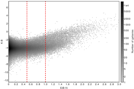
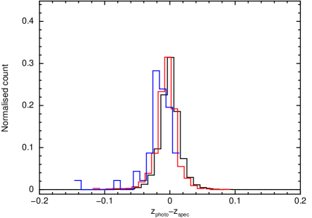
Figure 4: The effect of extinction on the colour and redshift accuracy of the 2MPZ V1.1 catalogue. Top: The extinction-corrected $K-B$ colour as a function of extinction. For values of $E(B-V)\geq 0.5$ a clear trend starts to emerge, indicating a selection effect due to reddening. The contours indicate the density of the points, and the red lines mark $E(B-V)=0.5$ and 1. Bottom: Histograms of $z_{\rm photo}-z{\rm spec}$ for objects with spectroscopic redshift measurements, for $E(B-V)<0.5$ (black), $0.5\leq E(B-V)<1$ (red) and $E(B-V)\geq 1$ (blue). The red histogram shows a small systematic shift, such that the mean photometric redshift is 0.004 too low compared to spectroscopic values; the widths are comparible. At high extinction, the photometric redshift calibration becomes very poor.

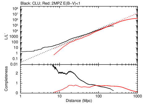
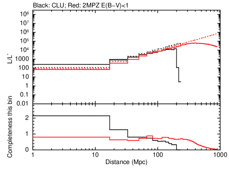
Figure 5: The completeness of the CLU (black) and 2MPZ V1.1 (red). In each plot the upper pane shows the theoretical total $L/L^{*}$ predicted by a Schechter function (dotted line) as a function of distance, and the observed value from the catalogues (solid line); the lower pane shows the ratio of the theoretical to observed, which we interpret as the completeness of the catalogue. The CLU data and theoretical values relate to $B$-band magnitudes. The 2MPZ data use $K$-band magnitudes. For 2MPZ, only sources in regions with $E(B-V)<1$ are included; the magnitudes have been corrected from isophotal to total values; see text for details. Left: Luminosity is integrated out to the distance on the x-axis, hence completeness refers to how complete the catalogue is out to distance D. Right: Luminosity is calculated in distance bins, hence completeness refers to how complete the catalogue is at distance D.

First, we must select an appropriate galaxy catalogue. Ideally this will be highly complete out to at least 500 Mpc, have uniform sky coverage, and reliable luminosity (in a single band) and distance measurements for every galaxy.

Gehrels et al. (2016) introduced the ‘Census of the Local Universe’ (CLU) catalogue, and Evans et al. (2016a) suggested the 2MASS Photometric Redshift catalogue [2MPZ; Bilicki et al. (2014) and Antolini & Heyl (2016) also suggested using 2MPZ]. The CLU is a meta catalogue created from several existing catalogues (Kasliwal, in preparation), whereas 2MPZ is based on a cross-correlation of the 2MASS extended source catalogue with the WISE and SuperCOSMOS all-sky catalogues. Following Gehrels et al. (2016) and earlier works (e.g. White et al. (2011)) we estimate the completeness of the catalogues by comparing the integrated luminosity observed out to a given distance, with that predicted by a Schechter function (Schechter, 1976). Using the terminology of Gehrels et al. (2016) we can define this function in terms of $x=L/L^{*}$ and the integrated luminosity per unit volume is therefore given by:

$$LdV=\int_{0}^{\infty}\phi^{*}L^{*}x^{\alpha+1}e^{-x}dx$$ (2)

where $L^{*}$, $\phi^{*}$ and $\alpha$ are measured from observations. For the $B$-band data used in the CLU, Gehrels et al. (2016) give $M_{B}^{*}=-19.7+5\log h$, $\alpha_{B}=-1.07$ and $\phi_{B}^{*}=0.016h^{3}$ ($M^{*}$ is the absolute magnitude of a galaxy with luminosity $L^{*}$); for 2MPZ we use the $K$-band magnitudes (as the catalogue is IR-selected) and the parameters from Kochanek et al. (2001): $M_{K}^{*}=-23.39+5\log h$, $\alpha_{B}=-1.09$ and $\phi_{B}^{*}=0.0116h^{3}$. We assumed $h=0.7(=H_{0}/100)$. To avoid questions of photometric zeropoints, rather than comparing the observed luminosity with that predicted by the Schechter function, we compare $x=L/L^{*}$, thus the zeropoints cancel out. From equation 2, the theoretical value for $x$ within volume $V$ is

$$x=\int_{0}^{\infty}\phi^{*}x^{\alpha+1}e^{-x}dxV=\phi^{*}\Gamma(\alpha+2,0)V$$ (3)

where $\Gamma$ is the incomplete gamma function.

The 2MPZ catalogue contains not the total infra-red magnitude of each galaxy, but instead those measured out to the 20mag/sq arcsec isophote (for the $K$ band, labelled as ‘k_m_k20fe’ in the 2MASS database). Such magnitudes will systematically miss some flux and need to be corrected for the total light. We follow Bilicki et al. (2011) and use the mean correction advocated by Kochanek et al. (2001), subtracting 0.2 mag from the $K$-band magnitudes of every entry in 2MPZ. We used a pre-release version 1.1 of 2MPZ. which contains $\sim\,$6,000 extra galaxies compared to 2MPZ (added after the correction of WISE instrumental artefacts), and the version we used contains more data that the public one as it had no cuts made for Galactic extinction or stellar density. Bilicki et al. (2014) noted that such cuts are important to preserve uniformity. At high extinction the dust maps of Schlegel et al. (1998) may saturate (i.e. become inaccurate); more significantly, at high extinction the intrinsically fainter galaxies become undetectable, and this is a function of wavelength, so intrinsically redder galaxies tend to be retained while bluer ones are lost, biasing the sample. In areas of high stellar density, where galaxies and stars may be blended, the colours can also become unreliable. For these reasons the publicly released catalogues (both v1 and v1.1) do not include sources for which $E(B-V)>1.5$ mag or log(stellar density, sources per square degree)$>$4.0; no such filters were applied to the dataset we began with (providing an extra 6,700 sources compared to the public dataset): we wish for a sample that is as homogeneous as possible, yet also accurate and complete, therefore we explored what cuts were necessary to achieve this. Fig. 4 shows the $K-B$ colour (both values are corrected for Galactic extinction) as a function of extinction, $E(B-V)$. A clear bias begins to emerge when the extinction exceeds 0.5 mag, demonstrating that the extinction correction, and therefore colours and hence photometric redshifts ($z_{\rm photo}$), are unreliable in this regime. The bottom panel of Fig. 4 shows the difference between the photometric redshift and spectroscopic redshift ($z_{\rm spec}$) for those objects with both, for three samples: $E(B-V)<0.5$, $0.5\leq E(B-V)<1$ and $E(B-V)\geq 1$. The $0.5\leq E(B-V)<1$ sample is slightly off-centre, suggesting that at these extinctions, $z_{\rm photo}$ is systematically underestimated by 0.004, however this shift is small compared to the uncertainty (discussed below) and can be ignored. There are only 46 objects in 2MPZ with a spectroscopic redshift and $E(B-V)\geq 1$ so we have not subdivided the data further for Fig. 4, however the effect of extinction on the distribution of photometric redshift is similar to that in Fig. 4; at higher extinctions, the distribution is biased towards ever lower photometric redshifts. While the number of galaxies at high extinctions is small compared to the overall catalogue, this clustering means that the inclusion of high-extinction objects significantly distorts the measurements of how complete the catalogue is. We therefore applied a cut of $E(B-V)<1$ to 2MPZ, resulting in 9,638 (1.0%) of the sources being discarded; all future discussion of 2MPZ in this work refers to this sample. We also investigated the effect that stellar density has on the accuracy of the catalogue. As with extinction, a clear bias in colour is visible at high stellar densities, however the extinction filtering just described removes all the sources with colours affected by stellar density, so an independent density filter is not needed.

In Fig. 5 we show the completeness of CLU and 2MPZ. At $D<40$Mpc, CLU is over-complete (i.e. contains more than the expected luminosity): this was also true of GWGC which White et al. (2011) attributed to the effect of the Virgo cluster. 2MPZ does not show this overcompleteness, this is likely the result both of the (comparatively) low sensitivity of 2MASS to low-surface-brightness galaxies (which dominate the nearby sample), and the inaccuracy of the photometric redshift: we return to the latter point below. Beyond $\sim\,$60 Mpc the 2MPZ survey is significantly more complete than CLU. 2MPZ also has the advantage of being more uniform across the sky than CLU; compare fig. 13 of Bilicki et al. (2014) with fig. 1 of Gehrels et al. (2016). In particular, completeness of CLU will depend on sky position, as this dataset is constructed from spectroscopic surveys, which at present do not cover the full sky beyond $\sim\,$130 Mpc [$z=0.03$: completeness of the 2MASS Redshift Survey, Huchra et al. (2012)]. Such a limitation does not apply to photometric all-sky surveys, such as 2MASS or WISE, which are only limited by their respective flux limits and Galactic plane nuisances.

These considerations suggest that 2MPZ represents the better catalogue to use, although if the GW information shows that the object is $<60$ Mpc away it may be better to instead use CLU.

However, the accuracy of the redshift information must also be considered. While CLU employs only spectroscopic redshift measurements, roughly 2/3 of the sources in 2MPZ have only photometric redshifts, which will have a larger uncertainty. To determine the accuracy of the photometric redshifts, we selected from 2MPZ only those objects with $E(B-V)<1$ and with both spectroscopic and photometric redshifts (the latter had the systematic correction above applied for $E(B-V)\geq 0.5$). We then created histograms of $z_{\rm photo}-z_{\rm spec}$ in several $z_{\rm photo}$ bins; two examples are shown in Fig. 6. These are approximately Gaussian, but the width ($\sigma_{z_{p}}$) varies with redshift. We fit this variation (Fig. 6, lower panel) with a broken powerlaw:

$$\sigma_{z_{p}}=\left\{\begin{array}[]{ll}0.043\ z_{\rm photo}^{0.402}&z_{\rm photo}<0.10\\ 0.023\ z_{\rm photo}^{0.14}&z_{\rm photo}\geq 0.10\\ \end{array}\right.$$ (4)

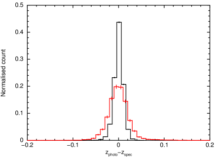
Figure 6: The accuracy of the photometric redshifts in 2MPZ. Top: Histograms of $z_{\rm photo}-z_{\rm spec}$ for galaxies with $z_{\rm photo}<0.05$ (black) and $0.2\leq z_{\rm photo}<0.25$ (red). Bottom: The variation of the Gaussian $\sigma$ of the histograms as a function of photometric redshift; the model is given in equation 4.

as shown in the lower panel of Fig. 6. This uncertainty must be taken into account when comparing the distance of a galaxy with the distance inferred from the GW data, as will be described in Section 3.2. This relatively large uncertainty in photometric redshift will also distort the completeness curve slightly. The probability of a galaxy with true redshift $z_{1}$ being assigned $z_{\rm photo}=z_{1}+\Delta z=z_{2}$ is slightly lower than the inverse: the probability of a galaxy with a true redshift $z_{2}$ being assigned $z_{\rm photo}=z_{2}-\Delta z=z_{1}$, because there is more volume (and so more galaxies) at $z_{2}$ than at $z_{1}$. This is clearly a bigger effect at lower redshift, where $\Delta z/z$ is higher. Similarly towards the limit of the catalogue’s redshift range (i.e. $z\to 0$ and $z\to z_{\rm lim}$) the completeness will be underestimated because some galaxies with true redshifts inside the catalogue’s redshift range will receive photometric values outside of it, but there are no (or few) galaxies outside of the limit to ‘compensate’. The overall effect of this is that the completeness shown in Fig. 5 is underestimated until the catalogue limit ($z\sim\,0.3$ corresponding to $D\sim\,1.6$ Gpc) is approached, i.e. 2MPZ is more complete within the distance range we are interested in than implied from Fig. 5, which strengthens the argument that 2MPZ is the better choice of the two catalogues we have studied. Looking further in the future as the horizon distance of aLIGO/AVIRGO rises further, we may wish to consider the forthcoming WISExSuperCOSMOS photometric redshift catalogue (Bilicki et al. 2016 in press), which covers less of sky than 2MPZ (70%), but reaches much deeper in redshift (median $z\sim\,0.2,D\sim\,850$ Mpc), however we defer study on the cost/benefit of this to a future work.

3.2 Using the distance and completeness

In our GW response to date, we have used galaxy catalogues in a simplistic way: we ignored the (in)completeness of the catalogue (i.e. regions of the sky without known galaxies were given zero probability of hosting the GW event) and did not weight galaxies by their distance compared to the expected distance to the GW event – the latter was not possible due to the lack of GW distance estimate available at trigger-time. In O2 and beyond, the horizon distance is such that the incompleteness of galaxy catalogues is significant (Fig. 5), and the aLIGO/VIRGO teams are likely to produce rapid distance estimates (Singer et al., 2016); therefore, we describe now a new method of galaxy convolution to produce higher-fidelity skymaps than we have used to date.

Considering first completeness: if the distance $D$ to the GW source is known perfectly, then we can estimate the completeness of the galaxy catalogue at this distance from the lower panel of Fig. 5, we will call this $C$. The probability that the GW event occurred in a known galaxy is thus $C$, and the probability that it occurred in an unknown one is $1-C$. Singer et al. (2016) demonstrated that the distance $D$ deduced from the GW data is a function of direction on the sky. The GW error regions are distributed as healpix-format skymaps, and each pixel in this map in the Singer et al. (2016) approach has its own $D$ distribution and hence $C$ value, which we calculate thus:

$$C_{p}=\frac{\int P_{p}(D)C(D)dD}{\int P_{p}(D)dD}$$ (5)

where $P_{p}(D)$ is the probability distribution of the distance, defined for the pixel $p$. Therefore, for each given pixel in the skymap, the probability of the GW event occurring in an uncatalogued galaxy within that pixel is:

$$\mathcal{P}_{{\rm nogal},p}=\mathcal{P}_{{\rm GW},p}\left(1-C_{p}\right)$$ (6)

where $\mathcal{P}_{{\rm GW},p}$ is the probability in the original skymap from the aLIGO/AVIRGO team for pixel $p$.

For pixels containing galaxies, an extra factor $\mathcal{P}_{{\rm gal},p}$ must be included. Previously (paper I) we defined this as in equation 1: the GW probability multiplied by the ratio of galaxy luminosity in the pixel to the total catalogued galaxy luminosity. This now needs to refer only to the luminosity within the distance indicated by the GW dataset, and needs a correction for completeness. We therefore redefine the probability of the GW event occurring within a known galaxy in pixel $p$ thus:

$$\mathcal{P}_{{\rm gal},p}=\mathcal{P}_{{\rm GW},p}C_{p}N\sum_{g}\left(\mathcal{P}(g|P_{p}[D])\frac{L_{g}}{L_{\rm tot}}\right)$$ (7)

The summation is over all galaxies $g$ in pixel $p$. $L_{g}$ is the luminosity of galaxy $g$ divided by the number of pixels it covers. $N$ is a normalisation needed to ensure that $\sum_{p}\mathcal{P}_{{\rm gal},p}=C$ (if $C$ is the catalogue completeness averaged over all pixels). This is given by:

$$N=\frac{\sum_{p}\mathcal{P}_{{\rm GW},p}C_{p}}{\sum_{p}\left(C_{p}\mathcal{P}_{{\rm GW},p}\sum_{g}{\left(\mathcal{P}(g|P_{p}[D])\frac{L_{g}}{L_{\rm tot}}\right)}\right)}$$ (8)

$L_{\rm tot}$ in equations (7)–(8) is the total catalogued galaxy luminosity within the GW volume, so $\sum_{g}\frac{L_{g}}{L_{\rm tot}}$ gives the ratio of the actual luminosity in pixel $p$ compared to the total distance-weighted luminosity of all galaxies in the GW error region, i.e. the relative probability of the galaxies in this pixel containing a merger event compared to those in any other pixel. $L_{\rm tot}$ is given by:

$$L_{\rm tot}=\sum_{p}\sum_{g}\left[\mathcal{P}(g|P_{p}[D])L_{g}\right]$$ (9)

where $\mathcal{P}(g|P(D)_{p})$ is the probability that the galaxy $g$ is at the correct distance to host the GW event. This is simply:

$$\mathcal{P}(g|P_{p}[D])=\int P_{p}(D)P_{g}(D)dD$$ (10)

where $P(D)_{p}$ is the probability as a function of distance for pixel P, determined from the GW data. For the low-latency analysis this is a Gaussian multiplied by distance squared (Singer et al., 2016). $P_{g}(D)$ is the probability distribution of the distance $D$ of galaxy $g$. 2MPZ does not contain uncertainties on the photometric redshift measurements, therefore we need to decide on the form of $P_{g}(D)$. For galaxies in 2MPZ with spectroscopic redshift we assume that the dominant source of error is the peculiar velocity of the galaxy, and we take 500 km s^-1 as representative of this. This corresponds to a distance error of $500/H_{0}=7.4$ Mpc (assuming $H_{0}=70$ km s^-1 Mpc^-1), so for galaxies with spectroscopic redshift we treat $P_{g}(D)$ as a Gaussian with $\sigma=7.4$ Mpc. For photometric redshifts we use the prescription given in Section 3.1 (the peculiar velocity correction is insignificant compared to this and can be ignored).

Having now calculated the probability of the GW event occurring in an unknown galaxy, or in any specific known galaxy, the probability that the GW event is in pixel $p$ of the skymap is simply:

$$\mathcal{P}_{p}=\mathcal{P}_{{\rm nogal},p}+\mathcal{P}_{{\rm gal},p}$$ (11)

Finally, the map must be renormalised such that it sums to unity. The result of this is a modified probability map on the sky which accounts for both the GW localisation and our prior knowledge of the structure of the local universe. This can then be used in a manner similar to that proposed by Gehrels et al. (2016), i.e. by selecting fields in (descending) probability order until some threshold probability has been selected (50% in the method of Gehrels et al. 2016). Alternatively, as suggested in Section 3, we can observe as many fields as possible in a given time interval, but again observing in order of priority.

Based on local structure in the universe it could be argued that the unknown galaxies are not homogeneously distributed on the sky, but are instead more likely near known galaxies. In this case, more exotic definitions of $P_{{\rm nogal},p}$ could be created to account for the distance to nearby galaxies. For the present, we will limit ourselves to the simple prescription above. Similarly since the values of binary inclination and distance determined from the GW are degenerate, the probability distribution of binary inclination for each pixel could in principle be produced and then, from a template library of GRB light curves for different inclinations, one could determine the probability of detecting a GRB from a given pixel as a function of time. While this is under investigation it is not likely to be possible on the timescale of O2, and is beyond the scope of this paper.

3.3 Which luminosity to use

The above calculations weigh each galaxy by its luminosity. However, which band one uses is also pertinent. The $K$-band provides a reasonable proxy for stellar mass in the galaxy, which we may take as being a proxy for the number of binary neutron-star systems in the galaxy and hence the probability of hosting a merger of such a system. However, recent observations (D’Avanzo et al., 2009; Fong et al., 2013) suggest that short GRBs are more common in late-type galaxies (suggesting that the probability of a compact binary coalescing is influenced by recent star formation), which suggest that it is more appropriate to weight galaxies by their $B$ band luminosity. 2MPZ contains both infrarad magnitudes (from 2MASS and WISE) and the optical $R$ and $B$ magnitudes (from SuperCOSMOS), which gives us the flexibility to select which band we wish to use, if the theoretical (or observation) priors change.

To investigate this, and the impact of the galaxy convolution, we performed a series of simulations. We started with the GW simulations of Singer et al. (2016), which provide 3-D probability maps for 250 simulated binary neutron star mergers in the 2-detector configuration. These simulations assume that the mergers are simply distributed homogeneously in space, whereas we wish to seed them in galaxies. Each GW simulation has the position and distance to the simulated event. We calculated the completeness $C$ of 2MPZ at this distance, and then generated a random number $0\leq\mathcal{R}<1$. If $\mathcal{R}\geq C$ the GW event was treated as occuring in an uncatalogued galaxy, so the data needed no changes. Otherwise, a host galaxy for the event was selected at random from the 2MPZ catalogue, with each galaxy having a probabilty of being the host, proportional to $L\mathcal{P}(D)$ (where $L$ is the galaxy luminosity and $\mathcal{P}(D)$ is the probability that this galaxy is at the distance of the simulated merger). Since the LIGO probability maps are strongly dependent on the geocentric direction to the merger, rather than rotate these maps such that the GW events occured in galaxies, instead we rotated the galaxy catalogue such that the selected host was at the position of the simulated merger. We then created a series of XRT fields tiled on the sky, arranged them in decreasing order of probability and determined which field contained the merger event.

We did this five times with different models. In the first instance, we performed no galaxy convolution at all, i.e. we simulated tiling the original GW error region. In the other four simulations, we selected host galaxies based on either their $B$- or $K$-band luminosities, and then convolved the GW map with 2MPZ using the $B$- or $K$-band luminosities. That is, we simulated the cases where our assumption about which galaxies are more likely to host GW events are correct (the same band was used in selecting the host and convolving the GW region), and when they are incorrect (one band was used to select the hosts, and the other used in convolution).

In Fig. 7 we show the results of this. Plotted is the cumulative distribution of which field contained the GRB in the 250 simulated mergers, for the different simulations runs. This confirms that the galaxy convolution significantly reduces the typical number of XRT fields we have to observe before we reach the correct location. With no convolution, 50% of the time at least 1,200 XRT fields are needed to reach the correct location. With convolution this falls to $\sim\,$170 (a factor of $\sim\,$7 decrease) if the same band is used in the simulations and search, or $\sim\,$300 fields (a factor of $\sim\,$4 improvement over the no-convolution approach) if different bands are used. Therefore, while the choice of which band to use when convolving galaxies does have a significant effect, choosing the wrong band is still much better than not using galaxy convolution.

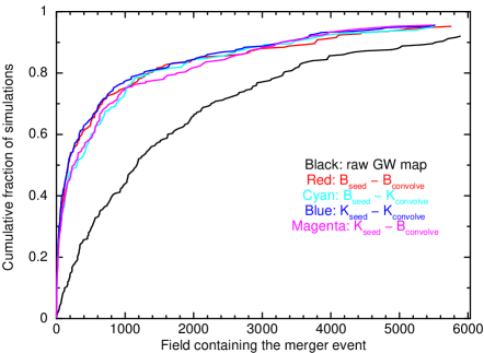
Figure 7: The cumulative distribution of which XRT field (in probability order) contains the GW event, from 250 simulated GW events (per colour), showing the benefit of galaxy convolution and the impact of using an incorrect assumption as to which luminosity band the galaxies should be weighted by. Black: Simulations where the XRT fields are generated based on the original GW map with no galaxy convolution. Red: The GW events are seeded in hosts weighted by $B$-band luminosity, and the GW error region is convolved with a $B$-band weighted galaxy catalogue. Cyan: Seeding is weighted by the $B$-band, but convolution uses the $K$-band. Blue: Seeding and convolution both use the $K$-band. Magenta: Seeding is weighted by the $K$-band and convolution by the $B$-band.

4 Conclusions

Swift performed rapid-response follow up to all three GW triggers released to the EM partners by the aLIGO team during the O1 operating run of aLIGO. No compelling X-ray, optical or gamma-ray counterpart was found, however this is not surprising, since only a small fraction of the GW error region was covered. Additionally, one of the GW triggers was spurious and the other two are believed to be BBH mergers, which may not be expected to give rise to EM emission. For the second trigger, we can place a limit on the hard X-ray emission of (4.3–90)$\times 10^{-8}$ erg

$$cm^{-2}\ s^{-1}(15--350keV)foraregionenclosing15\%\ oftheGWprobability.\par Inthefuture\emph{Swift}\ willbeabletoobserveamuchlargerfractionoftheGWerrorregionasanewobservingcapabilityhasbeencommissioned,whichwillenablelarge-scale,short-exposuretiling.GivenboththeincreasedhorizondistanceexpectedduringO2,andthefactthatbothrealGWeventsinO1wereatlargedistances(\sim\,500Mpc),targetinggalaxiesintheGWGC,whichislimitedto100Mpc,isnotagoodapproach.The2MPZcatalogue,whichusesamixtureofspectroscopicandphotometricredshifts,offersabetterprospect(unlesstheGWlocalisationidentifiestheobjectasbeing<60MpcfromEarth),andwehaveshownhowwecanusethecompletenessmeasurementsforthiscatalogue,andtheGWdistanceestimatesexpectedtoberapidlyavailableinO2,tooptimisetheskymapproducedbytheaLIGO/AVIRGOteams.Inthefuture,asnewcataloguesbecomeavailable(suchastheWISExSuperCOSMOS,GLADEinprep/press)orwhenphotometricredshiftsareaddedtoWise-2MASScomplilation\cite[citep]{(\@@bibref{AuthorsPhrase1Year}{Kovacs15}{\@@citephrase{, }}{})},andthesensitivityandlocalisationcharacteristicsofaLIGO/AVIRGOimproveitmaybevaluabletoreassessthebenefitsofgalaxytargetingandchoiceofcatalogue.\par\par\par\par$$

References

- Abbott et al. (2016a) Abbott B. P., et al., 2016a, preprint (arXiv:1602.08492)
- Abbott et al. (2016b) Abbott B. P., et al., 2016b, Technical Report LIGO-P1600088, https://dcc.ligo.org/LIGO-P1600088/public/main. https://dcc.ligo.org/LIGO-P1600088/public/main
- Abbott et al. (2016c) Abbott B. P., et al., 2016c, Living Reviews in Relativity, 19
- Abbott et al. (2016d) Abbott B. P., et al., 2016d, Phys. Rev. Lett., 116, 061102
- Abbott et al. (2016e) Abbott B. P., et al., 2016e, Phys. Rev. Lett., 116, 241103
- Abbott et al. (2016f) Abbott B. P., et al., 2016f, Physical Review Letters, 116, 131103
- Acernese et al. (2015) Acernese F., et al., 2015, Classical and Quantum Gravity, 32, 024001
- Antolini & Heyl (2016) Antolini E., Heyl J. S., 2016, preprint, (arXiv:1602.07710)
- Barthelmy et al. (2005) Barthelmy S. D., et al., 2005, Space Sci. Rev., 120, 143
- Berger (2014) Berger E., 2014, ARA&A, 52, 43
- Bilicki et al. (2011) Bilicki M., Chodorowski M., Jarrett T., Mamon G. A., 2011, ApJ, 741, 31
- Bilicki et al. (2014) Bilicki M., Jarrett T. H., Peacock J. A., Cluver M. E., Steward L., 2014, ApJS, 210, 9
- Burrows et al. (2005) Burrows D. N., et al., 2005, Space Sci. Rev., 120, 165
- Burrows et al. (2006) Burrows D. N., et al., 2006, ApJ, 653, 468
- Chambers et al. (2015) Chambers K. C., et al., 2015, Gamma Ray Coordinates Network Circular, 18811
- Connaughton et al. (2016) Connaughton V., et al., 2016, preprint, (arXiv:1602.03920)
- D’Avanzo et al. (2009) D’Avanzo P., et al., 2009, A&A, 498, 711
- Evans et al. (2014) Evans P. A., et al., 2014, ApJS, 210, 8
- Evans et al. (2015a) Evans P. A., et al., 2015a, Gamma Ray Coordinates Network Circular, 18331
- Evans et al. (2015b) Evans P. A., et al., 2015b, Gamma Ray Coordinates Network Circular, 18346
- Evans et al. (2015c) Evans P. A., et al., 2015c, Gamma Ray Coordinates Network Circular, 18446
- Evans et al. (2015d) Evans P. A., et al., 2015d, Gamma Ray Coordinates Network Circular, 18489
- Evans et al. (2015e) Evans P. A., et al., 2015e, Gamma Ray Coordinates Network Circular, 18569
- Evans et al. (2015f) Evans P. A., et al., 2015f, Gamma Ray Coordinates Network Circular, 18732
- Evans et al. (2015g) Evans P. A., et al., 2015g, Gamma Ray Coordinates Network Circular, 18733
- Evans et al. (2015h) Evans P. A., et al., 2015h, Gamma Ray Coordinates Network Circular, 18748
- Evans et al. (2015i) Evans P. A., et al., 2015i, Gamma Ray Coordinates Network Circular, 18834
- Evans et al. (2015j) Evans P. A., et al., 2015j, Gamma Ray Coordinates Network Circular, 18870
- Evans et al. (2016a) Evans P. A., et al., 2016a, MNRAS, 455, 1522
- Evans et al. (2016b) Evans P. A., et al., 2016b, MNRAS, 460, L40
- Fan et al. (2014) Fan X., Messenger C., Heng I. S., 2014, ApJ, 795, 43
- Fong et al. (2013) Fong W., et al., 2013, ApJ, 769, 56
- Fong et al. (2015) Fong W., Berger E., Margutti R., Zauderer B. A., 2015, ApJ, 815, 102
- Gehrels et al. (2004) Gehrels N., et al., 2004, ApJ, 611, 1005
- Gehrels et al. (2016) Gehrels N., Cannizzo J. K., Kanner J., Kasliwal M. M., Nissanke S., Singer L. P., 2016, ApJ, 820, 136
- Górski et al. (2005) Górski K. M., Hivon E., Banday A. J., Wandelt B. D., Hansen F. K., Reinecke M., Bartelmann M., 2005, ApJ, 622, 759
- Grupe et al. (2006) Grupe D., Burrows D. N., Patel S. K., Kouveliotou C., Zhang B., Mészáros P., Wijers R. A. M., Gehrels N., 2006, ApJ, 653, 462
- Huchra et al. (2012) Huchra J. P., et al., 2012, ApJS, 199, 26
- Kamble & Kaplan (2013) Kamble A., Kaplan D. L. A., 2013, International Journal of Modern Physics D, 22, 1341011
- Kanner et al. (2013) Kanner J., Baker J., Blackburn L., Camp J., Mooley K., Mushotzky R., Ptak A., 2013, ApJ, 774, 63
- Kochanek et al. (2001) Kochanek C. S., et al., 2001, ApJ, 560, 566
- Kovács & Szapudi (2015) Kovács A., Szapudi I., 2015, MNRAS, 448, 1305
- LIGO Scientific Collaboration (2015a) LIGO Scientific Collaboration 2015a, Gamma Ray Coordinates Network Circular, 18626
- LIGO Scientific Collaboration (2015b) LIGO Scientific Collaboration 2015b, Gamma Ray Coordinates Network Circular, 18851
- LIGO Scientific Collaboration (2015c) LIGO Scientific Collaboration 2015c, Gamma Ray Coordinates Network Circular, 18853
- LIGO Scientific Collaboration & VIRGO (2015) LIGO Scientific Collaboration VIRGO 2015, Gamma Ray Coordinates Network Circular, 18889
- LIGO Scientific Collaboration et al. (2013) LIGO Scientific Collaboration et al., 2013, preprint, (arXiv:1304.0670)
- LIGO Scientific Collaboration et al. (2015) LIGO Scientific Collaboration et al., 2015, Classical and Quantum Gravity, 32, 074001
- Li & Paczyński (1998) Li L.-X., Paczyński B., 1998, ApJ, 507, L59
- Loeb (2016) Loeb A., 2016, ApJ, 819, L21
- Lyutikov (2016) Lyutikov M., 2016, preprint, (arXiv:1602.07352)
- Metzger & Berger (2012) Metzger B. D., Berger E., 2012, Astrophys. J., 746, 48
- Nakar & Piran (2011) Nakar E., Piran T., 2011, Nature, 478, 82
- Perna et al. (2016) Perna R., Lazzati D., Giacomazzo B., 2016, preprint, (arXiv:1602.05140)
- Piranomonte et al. (2015) Piranomonte S., et al., 2015, Gamma Ray Coordinates Network Circular, 18488
- Rabinowitz et al. (2015a) Rabinowitz D., C. B., Ellman N., Woodward E., Nugent P., 2015a, Gamma Ray Coordinates Network Circular, 18473
- Rabinowitz et al. (2015b) Rabinowitz D., et al., 2015b, Gamma Ray Coordinates Network Circular, 18572
- Roming et al. (2005) Roming P. W. A., et al., 2005, Space Sci. Rev., 120, 95
- Savchenko et al. (2016) Savchenko V., et al., 2016, ApJ, 820, L36
- Schechter (1976) Schechter P., 1976, ApJ, 203, 297
- Schlegel et al. (1998) Schlegel D. J., Finkbeiner D. P., Davis M., 1998, ApJ, 500, 525
- Singer & Price (2016) Singer L. P., Price L. R., 2016, Phys. Rev. D, 93, 024013
- Singer et al. (2014) Singer L. P., et al., 2014, Astrophys. J., 795, 105
- Singer et al. (2015a) Singer L., et al., 2015a, Gamma Ray Coordinates Network Circular, 18442
- Singer et al. (2015b) Singer L. P., Kasliwal M. M., Ferretti R., Cenko S. B., Barlow T., Cao Y., Laher R., Rana J., 2015b, Gamma Ray Coordinates Network Circular, 18497
- Singer et al. (2016) Singer L. P., et al., 2016, preprint, (arXiv:1603.07333)
- The LIGO Scientific Collaboration et al. (2016) The LIGO Scientific Collaboration et al., 2016, preprint, (arXiv:1602.03839)
- Troja et al. (2010) Troja E., Rosswog S., Gehrels N., 2010, ApJ, 723, 1711
- Troja et al. (2016) Troja E., et al., 2016, preprint, (arXiv:1605.03573)
- Tsang (2013) Tsang D., 2013, ApJ, 777, 103
- Veitch et al. (2015) Veitch J., et al., 2015, Phys. Rev. D, 91, 042003
- Voges et al. (1999) Voges W., et al., 1999, A&A, 349, 389
- White et al. (2011) White D. J., Daw E. J., Dhillon V. S., 2011, Class. Quantum Gravity, 28, 085016
- Yamazaki et al. (2016) Yamazaki R., Asano K., Ohira Y., 2016, preprint, (arXiv:1602.05050)
- Zhang (2013) Zhang B., 2013, ApJ, 763, L22
- Zhang (2016) Zhang B., 2016, preprint, (arXiv:1602.04542)
- Zhang et al. (2015) Zhang B.-B., van Eerten H., Burrows D. N., Ryan G. S., Evans P. A., Racusin J. L., Troja E., MacFadyen A., 2015, ApJ, 806, 15