Distance geometry approach for special graph coloring problems

Rosiane de Freitas Instituto de Computação, Universidade Federal do Amazonas, Av. Rodrigo Otávio 3000, 69000-000, Manaus, Brazil Bruno Dias Instituto de Computação, Universidade Federal do Amazonas, Av. Rodrigo Otávio 3000, 69000-000, Manaus, Brazil Nelson Maculan COPPE, Universidade Federal do Rio de Janeiro, C.P. 68530, 21945-970, Rio de Janeiro, Brazil Jayme Szwarcfiter COPPE, Universidade Federal do Rio de Janeiro, C.P. 68530, 21945-970, Rio de Janeiro, Brazil

Abstract

One of the most important combinatorial optimization problems is graph coloring. There are several variations of this problem involving additional constraints either on vertices or edges. They constitute models for real applications, such as channel assignment in mobile wireless networks. In this work, we consider some coloring problems involving distance constraints as weighted edges, modeling them as distance geometry problems. Thus, the vertices of the graph are considered as embedded on the real line and the coloring is treated as an assignment of positive integers to the vertices, while the distances correspond to line segments, where the goal is to find a feasible intersection of them. We formulate different such coloring problems and show feasibility conditions for some problems. We also propose implicit enumeration methods for some of the optimization problems based on branch-and-prune methods proposed for distance geometry problems in the literature. An empirical analysis was undertaken, considering equality and inequality constraints, uniform and arbitrary set of distances, and the performance of each variant of the method considering the handling and propagation of the set of distances involved.

Keywords: branch-and-prune; channel assignment; constraint propagation; graph theory; T-coloring.

1 Introduction

Let $G=(V,E)$ be an undirected graph. A $k$ -coloring of $G$ is an assignment of colors $\{1,2,\dots,k\}$ to the vertices of $G$ so that no two adjacent vertices share the same color. The chromatic number $\chi_{G}$ of a graph is the minimum value of $k$ for which $G$ is $k$ -colorable. The classic graph coloring problem, which consists in finding the chromatic number of a graph, is one of the most important combinatorial optimization problems and it is known to be NP-hard (Karp, 1972).

There are several versions of this classic vertex coloring problem, involving additional constraints, in both edges as vertices of the graph, with a number of practical applications as well as theoretical challenges. One of the main applications of such problems consists of assigning channels to transmitters in a mobile wireless network. Each transmitter is responsible for the calls made in the area it covers and the communication among devices is made through a channel consisting of a discrete slice of the electromagnetic spectrum. However, the channels cannot be assigned to calls in an arbitrary way, since there is the problem of interference among devices located near each other using approximate channels. There are three main types of interferences: co-channel, among calls of two transmitters using the same channels; adjacent channel, among calls of two transmitters using adjacent channels and co-site, among calls on the same cell that do not respect a minimal separation. It is necessary to assign channels to the calls such that interference is avoided and the spectrum usage is minimized (Audhya et al., 2011; Koster and Munhoz, 2010; Koster, 1999).

Thus, the channel assignment scenario is modeled as a graph coloring problem by considering each transmitter as a vertex in a undirected graph and the channels to be assigned as the colors that the vertices will receive. Some more general graph coloring problems were proposed in the literature in order to take the separation among channels into account, such as the T-coloring problem, also known as the Generalized Coloring Problem (GCP) where, for each edge, the absolute difference between colors assigned to each vertex must not be in a given forbidden set (Hale, 1980). The Bandwidth Coloring Problem, a special case of T-coloring where the absolute difference between colors assigned to each vertex must be greater or equal a certain value (Malaguti and Toth, 2010), and the coloring problem with restrictions of adjacent colors (COLRAC), where there is a restriction graph for which adjacent colors in it cannot be assigned to adjacent vertices (Akihiro et al., 2002).

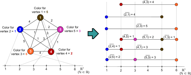
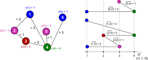
The separation among channels is a type of distance constraint, so we can see the channel assignment as a type of distance geometry (DG) problem (Liberti et al., 2014) since we have to place the channels in the transmitters respecting some distances imposed in the edges, as can be seen in Figure 1. One method to solve DG problems is the branch-and-prune approach proposed by Lavor et al. (2012a, b), where a solution is built and if at some point a distance constraint is violated, then we stop this construction (prune) and try another option for the current solution in the search space. See also: Mucherino et al. (2013); Lavor et al. (2012a); Freitas et al. (2014a, b); Dias (2014); Dias et al. (2013, 2012).

For graph theoretic concepts and terminology, see the book by Bondy and Murty (2008).

The main contribution of this paper consists of a distance geometry approach for special cases of T-coloring problems with distance constraints, involving a study of graph classes for which some of these distance coloring problems are unfeasible, and branch-prune-and-bound algorithms, combining concepts from the branch-and-bound method and constraint propagation, for the considered problems.

The remainder of this paper is organized as follows. Section 2 defines the distance geometry models for some special graph coloring problems. Section 3 shows some properties regarding the structure of those distance geometry graph coloring problems, including the determination of feasibility for some graphs classes. Section 4 formulates the branch-prune-and-bound (BPB) algorithms proposed for the problems and shows properties regarding optimality results. Section 5 shows results of some experiments done with the BPB algorithms using randomly generated graphs for each proposed model. Finally, Section 6 concludes the paper and states the next steps for ongoing research.

Refer to caption — Figure 1: Example of channel assignment with distance constraints, where the separation is given by the weight in each edge. The image on the right shows the network as an undirected graph and the projection of vertices on the real number line, but considering only natural numbers.

2 Distance geometry and graph colorings

We propose an approach in distance geometry for special vertex coloring problems with distance constraints, based on the Discretizable Molecular Distance Geometry Problem (DMDGP), which is a special case of the Molecular Distance Geometry Problem, where the set $V$ of vertices from the input graph $G$ are ordered such that the set $E$ of edges contain all cliques on quadruplets of consecutive vertices, that is, any four consecutive vertices induce a complete graph ( $\forall i\in\{4,\dots,n\}\ \forall j,k\in\{i-3,\dots,i\}\ (\{j,k\}\in E)$ ) (Lavor et al., 2012a). Furthermore, a strict triangular inequality holds on weights of edges between consecutive vertices in such ordering ( $\forall i\in\{2,\dots,n-1\}\ d_{i-1,i+1}<d_{i-1,i}\ +\ d_{i,i+1}$ ). All coordinates are given in $\mathbb{R}^{3}$ space. The position for a point $i$ (where $i\geq 4$ ) can be determined using the positions of the previous three points $i-1,i-2$ and $i-3$ by intersecting three spheres with radii $d_{i-3,i},d_{i-2,i}$ and $d_{i-1,i}$ , obtaining two possible points that are checked for feasibility.

A similar reasoning can be used in vertex coloring problems with distance constraints, where the distances that must be respected involve the absolute difference between two values $x(i)$ and $x(j)$ (respectively, the color points attributed to $i$ and $j$ ), but for these problems the space considered is actually unidimensional. The positioning of a vertex $i$ can be determined by using a neighbor $j$ that is already positioned. Thus, we have a 0-sphere, consisting of a projection of a 1-sphere (a circle), which itself is a projection of a 2-sphere (the three-dimensional sphere), as shown in Figure 2. The 0-sphere is a line segment with a radius $d_{i,j}$ , and feasible colorings consist of treating the intersections of these 0-spheres. Figure 3 exemplifies the correlations between these types of spheres and shows the example from Figure 1 as the positioning of these line segments.

In this work we focus on problems with exact distances between colors, and also in the analysis of different types of BPB algorithms and integer programming models.

Based on DMDGP, which is a decision problem involving equality distance constraints, the basic distance graph coloring model we consider also involves equality constraints between colors of two neighbor vertices $i$ and $j$ . That is, the absolute difference between them must be exactly equal to an arbitrary weight imposed on the edge $(i,j)$ , and the solution candidate must satisfy all given constraints. We can formally define as follows.

Given a graph $G=(V,E)$ , we define $d_{i,j}$ as a positive integer weight associated to an edge $(i,j)\in E(G)$ . In distance coloring, for each vertex $i$ , a color must be determined for it (denoted by $x(i)$ ) such that the constraints imposed on the edges between $i$ and its neighbors are satisfied. A variation of the classic graph coloring problem consists in finding the minimum span of $G$ , that is, in determining that the maximum $x(i)$ , or color used, be the minimum possible. Based on these preliminary definitions, we describe the following distance geometry vertex coloring problems.

Definition 1.

Coloring Distance Geometry Problem (CDGP): Given a simple weighted undirected graph $G=(V,E)$ , where, for each $(i,j)\in E$ , there is a weight $d_{i,j}\in\mathbb{N}$ , find an embedding $x:V\rightarrow\mathbb{N}$ (that is, an embedding of $G$ on the real number line, but considering only the natural number points) such that $|x(i)-x(j)|=d_{i,j}$ for each $(i,j)\in E$ .

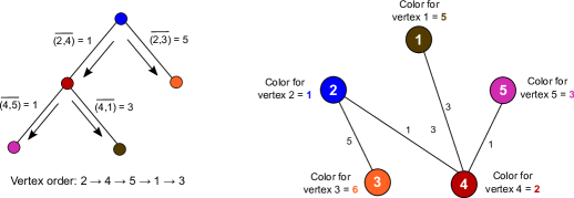
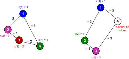
CDGP involves equality constraints, and thus is named as Equal Coloring Distance Geometry Problem and labeled as EQ-CDGP. A solution for this problem consists of a tree, whose vertices are colored with colors that respect the equality constraints involving the weighted edges (see Figure 4). Since CDGP (or EQ-CDGP) is a decision problem, only a feasible solution is required. This problem is NP-complete, as shown below.

Theorem 1.

EQ-CDGP is NP-complete.

Proof.

To prove that EQ-CDGP $\in$ NP-complete, we must show that EQ-CDGP $\in$ NP and EQ-CDGP $\in$ NP-hard.

1. EQ-CDGP $\in$ NP.
Given, for a graph $G=(V,E)$ , an embedding $x:V\rightarrow\mathbb{N}$ , its feasibility can be checked by taking each edge $(i,j)\in E$ and examining if its endpoints do not violate the corresponding distance constraint, that is, if $|x(i)-x(j)|=d_{i,j}$ . If all distance constraints are valid, then $x$ is a certificate for a positive answer to the EQ-CDGP instance, meaning that a certificate for a YES answer can be verified in $O(|E|)$ time, which is linear. Thus, EQ-CDGP $\in$ NP.

2. EQ-CDGP $\in$ NP-hard.
Since EQ-CDGP is equivalent to 1-Embeddability with integer weights, which is NP-hard (Saxe, 1979), we can use the same proof for the latter problem to show that EQ-CDGP is also NP-hard. The proof is made by reducing the Partition problem, which is known to be NP-complete (Garey and Johnson, 1979) to EQ-CDGP.
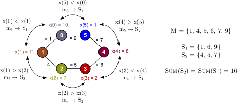
Consider a Partition instance, consisting of a set $I$ of $r$ integers, that is, $M=\{m_{1},m_{2},\dots,m_{r}\}$ . Let $G$ be a weighted graph $G=(V,E)$ , where $G$ is a cycle such that $|V|=|E|=r$ and, for each edge $(i,j)$ , its weight is a natural number denoted by $d_{i,j}$ . This graph is constructed from $M$ by considering:

•

$V=\{i_{0},i_{1},\dots,i_{r-1}\}.$
•

$E=\{(i_{b},i_{b+1\text{ mod }r})\ |\ 0\leq b\leq r\}.$
•

$d_{i_{b},i_{b+1\text{ mod }r}}=m_{b}\ (\forall 0\leq b\leq r).$

Now, let $x:V\rightarrow\mathbb{N}$ be an embedding of the vertices on the number line. If it is a valid embedding, then we can define two sets:

•

$S_{1}=\{m_{b}\ |\ x(i_{b})<x(i_{b+1\text{ mod }r})\}$ .
•

$S_{2}=\{m_{b}\ |\ x(i_{b})>x(i_{b+1\text{ mod }r})\}$ .

We have that $S_{1}$ and $S_{2}$ are disjoint subsets of $M$ (that is, they form a partition of $M$ ) where the sum of all $S_{1}$ elements is equal to the sum of all $S_{2}$ elements, that is, if the cyclic graph constructed from $G$ admits an embedding on the line (which means that its solution to EQ-CDGP is YES), then $M$ has a YES solution for Partition and vice-versa. This reduction can be made in $O(r)$ time, thus, EQ-CDGP $\in$ NP-hard. ∎

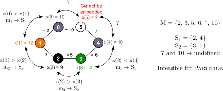
To illustrate the reasoning from Theorem 1, let $M$ be an instance of Partition such that $M=\{1,4,5,6,7,9\}$ . Figure 5 shows its corresponding EQ-CDGP solution.

Since most graph coloring problems in the literature and in real world applications are optimization problems, we define an optimization version of this basic distance geometry graph coloring problem, as shown below.

Definition 2.

Minimum Equal Coloring Distance Geometry Problem (MinEQ-CDGP): Given a simple weighted undirected graph $G=(V,E)$ , where, for each $(i,j)\in E$ , there is a weight $d_{i,j}\in\mathbb{N}$ , find an embedding $x:V\rightarrow\mathbb{N}$ such that $|x(i)-x(j)|=d_{i,j}$ for each $(i,j)\in E$ whose span $S$ , defined as $S=\max_{i\in V}x(i)$ , that is, the maximum used color, is the minimum possible.

Figure 6 shows an example of this model and its corresponding 0-sphere visualization.

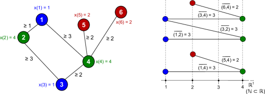
On the other hand, instead of equalities, we can consider inequalities, such that the weight $d_{i,j}$ on an edge $(i,j)$ is actually a lower bound for the distance to be respected between the color points $x(i)$ and $x(j)$ , that is, $|x(i)-x(j)|\geq d_{ij}$ . Thus, we can modify MinEQ-CDGP to deal with this scenario, which becomes the following model.

Definition 3.

Minimum Greater than or Equal Coloring Distance Geometry Problem(MinGEQ-CDGP): Given a simple weighted undirected graph $G=(V,E)$ , where, for each $(i,j)\in E$ , there is a weight $d_{i,j}\in\mathbb{N}$ , find an embedding $x:V\rightarrow\mathbb{N}$ such that $|x(i)-x(j)|\geq d_{i,j}$ for each $(i,j)\in E$ whose span ( $\max\limits_{i\in V}x(i)$ ) is the minimum possible.

MinGEQ-CDGP is equivalent to the bandwidth coloring problem (BCP) (Malaguti and Toth, 2010), which itself is equivalent to the minimum span frequency assignment problem (MS-FAP) (Koster, 1999; Audhya et al., 2011).

Figure 6 In Figure 7, this model, along with its 0-sphere representation, is exemplified.

2.1 Special cases

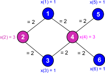
For the models previously stated, we can identify some specific scenarios for which additional properties can be identified. The first special case is for EQ-CDGP, the decision distance coloring problem, where all distances are the same, that is, the input is a graph with uniform edge weights, as stated below.

Definition 4.

Coloring Distance Geometry Problem with Uniform Distances (EQ-CDGP-Unif): Given a simple weighted undirected graph $G=(V,E)$ , and a nonnegative integer $\varphi$ , find an embedding $x:V\rightarrow\mathbb{N}$ such that $|x(i)-x(j)|=\varphi$ for each $(i,j)\in E$ .

For the optimization version, we can also define this special case, as shown below.

Definition 5.

Minimum Equal Coloring Distance Geometry Problem with Uniform Distances (MinEQ-CDGP-Unif): Given a simple weighted undirected graph $G=(V,E)$ , and a nonnegative integer $\varphi$ , find an embedding $x:V\rightarrow\mathbb{N}$ such that $|x(i)-x(j)|=\varphi$ for each $(i,j)\in E$ whose span ( $\max_{i\in V}x(i)$ ) is the minimum possible.

In this model, an input graph can be defined by its sets of vertices and edges and the $\varphi$ value, instead of a set of weights for each edge. A similar special case exists for MinGEQ-CDGP, as stated in the following definition.

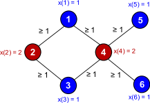
Definition 6.

Minimum Greater than or Equal Coloring Distance Geometry Problem with Uniform Distances (MinGEQ-CDGP-Unif): Given a simple weighted undirected graph $G=(V,E)$ , and a nonnegative integer $\varphi$ , find an embedding $x:V\rightarrow\mathbb{N}$ such that $|x(i)-x(j)|\geq\varphi$ for each $(i,j)\in E$ whose span ( $\max_{i\in V}x(i)$ ) is the minimum possible.

When $\varphi=1$ , MinGEQ-CDGP-Unif is equivalent to the classic graph coloring problem (Figure 8).

A summary of all distance coloring models, including special cases, is given in Table 1.

Table 1: Summary of distance coloring models.

Problem	Constraint type	Distance type
EQ-CDGP and MinEQ-CDGP	$\forall(i,j)\in E,\ \|x(i)-x(j)\|=d_{i,j}$	$\forall(i,j)\in E,\ d_{i,j}\in\mathbb{N}$
MinGEQ-CDGP	$\forall(i,j)\in E,\ \|x(i)-x(j)\|\geq d_{i,j}$	$\forall(i,j)\in E,\ d_{i,j}\in\mathbb{N}$
EQ-CDGP-Unif and MinEQ-CDGP-Unif	$\forall(i,j)\in E,\ \|x(i)-x(j)\|=d_{i,j}$	$\forall(i,j)\in E,\ d_{i,j}=\varphi$ $(\varphi\in\mathbb{N})$
MinGEQ-CDGP-Unif	$\forall(i,j)\in E,\ \|x(i)-x(j)\|\geq d_{i,j}$	$\forall(i,j)\in E,\ d_{i,j}=\varphi$ $(\varphi\in\mathbb{N})$

3 Feasibility conditions of distance graph coloring problems

In this section, we discuss feasibility conditions related to our proposed EQ-CDGP problems. Clearly, the problems involving inequality constraints are always feasible. This is the case for the MinGEQ-CDGP and MinGEQ-CDGP problems (and the special cases with uniform distances, MinGEQ-CDGP-Unif and MinGEQ-CDGP-Unif). However, this is not so for versions that involve only equality constraints, EQ-CDGP and its special case with uniform distances, the EQ-CDGP-Unif problem.

3.1 Feasibility conditions for EQ-CDGP-Unif

Graphs that admit a solution for the EQ-CDGP-Unif problem are characterized by the following theorem.

Theorem 2.

A graph $G$ has solution YES for EQ-CDGP-Unif problem if and only if $G$ is bipartite.

Proof.

Let $G$ be a graph, input to a EQ-CDGP-Unif problem, where for each edge $v_{i}v_{j}$ of $G$ , the distance required is $d_{ij}=\varphi$ , $\varphi\in\mathbb{N}$ , constant. Suppose $G$ has a YES solution for the problem such that $x:V\rightarrow\mathbb{N}$ is a certificate for that solution. Let $x(i)$ be the color assigned to $v_{i}\in V$ . Choose an arbitrary path $v_{1},v_{2},...,v_{k}$ of $G$ , not necessarily simple. Then $|x(i)-x(j)|=\varphi$ , for $|i-j|=1$ . The latter implies $x(i)=x(i+2)$ , $i=1,2,...,k-2$ . Consequently, if the path contains the same vector $v_{i}$ twice, their corresponding indices are the same. That is, all edges of $G$ are necessarily even, and $G$ is bipartite.

Conversely, if $G$ is bipartite, its vertices admit a proper coloring with two distinct colors. Assign the value $x(i)$ to the vertices of the first color, and the value $\varphi+1$ to the second one. Then $|x(i)-x(j)|=\varphi$ , for each edge $v_{i}v_{j}$ of $G$ , and EQ-CDGP-Unif has a YES solution. As an alternative way of proving that if a graph is bipartite then it has a YES solution for EQ-CDGP, observe that, since the input graph is bipartite, it is also 2-colorable (considering the classic graph coloring problem), that is, the entire graph can be colored using only two different colors, which can be determined by considering a single edge from the graph. All edges $(i,j)$ have the same distance constraint, that is, $|x(i)-x(j)|=\varphi$ , so the two colors that will be used are {1, 1+ $\varphi$ }, which form the solution for the EQ-CDGP-Unif instance.

In order to prove the converse statement, that is, if a graph has a YES solution for EQ-CDGP, it is bipartite, we will use a proof by contrapositive, which states that if a graph is not bipartite, then it has a NO solution for EQ-CDGP. This will be done by mathematical induction on odd cycles, since a graph is not bipartite if, and only if, it contains an odd cycle. Let $|V|=2z+1$ . The proof will be by induction on $z$ (the number of vertices).

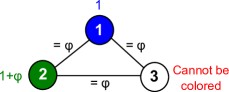
Base case: $z=1$ . We have the cycle $C_{3}$ , with three vertices ( $V=\{1,2,3\}$ ) and three edges ( $\{(1,2),(1,3),(2,3)\}$ ), with $|x(i)-x(j)|=\varphi$ for all of them. Without loss of generality, let $x(1)=1$ and $x(2)=1+\varphi$ . Then we have that:

•

Since $(1,3)\in E$ and $x(1)=1$ , then $|x(3)-1|=\varphi$ . All colors must be positive integers, so $x(3)=1+\varphi$ .
•

Since $(2,3)\in E$ and $x(2)=1+\varphi$ , then $|x(3)-(1+\varphi)|=\varphi\ \ \Rightarrow\ \ |x(3)-1-\varphi|=\varphi$ . By this inequation, $x(3)=1$ or $x(3)=1+2\varphi$ .

From this result, we have that $x(3)=1+\varphi$ and ( $x(3)=1$ or $x(3)=1+2\varphi$ ) at the same time, which is impossible. Then $C_{3}$ has a NO solution for EQ-CDGP, as seen in Figure 9.

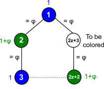
Induction hypothesis: The cycle $C_{2z+1}$ has a NO solution for EQ-CDGP.

Inductive step: By the inductive hypothesis, the cycle $C_{2z+1}$ is infeasible for EQ-CDGP. If we consider the cycle $C_{2(z+1)+1}=C_{2z+3}$ , we have that the size of the cycle increases by two vertices, but it will still be an odd cycle. If we add only one vertex, that is, we consider the cycle $C_{2z+1+1}=C_{2z+2}$ , we will have an even cycle. Since all even cycles are bipartite, they are feasible in EQ-CDGP according to Theorem 2. Now, consider that another vertex is added to $C_{2z+2}$ , becoming $C_{2z+3}$ . Without loss of generality, consider that the new vertex $2z+3$ is adjacent to vertices $2z+2$ and $1$ , that is, we have $\{(2z+2,2z+3),(2z+3,1)\}\subseteq E$ , and $x(2z+2)=1+\varphi$ and $x(1)=1$ (these colors can be seen as having been assigned when we added only one vertex, generating an even cycle). Then we have that:

•

Since $(2z+2,2z+3)\in E$ and $x(2z+2)=1+\varphi$ , then $|x(2z+3)-(1+\varphi)|=\varphi\ \ \Rightarrow\ \ |x(2z+3)-1-\varphi|=\varphi$ . By this inequation, $x(2z+3)=1$ or $x(2z+3)=1+2\varphi$ .
•

Since $(2z+3,1)\in E$ and $x(1)=1$ , then $|x(2z+3)-1|=\varphi$ . All colors must be positive integers, so $x(2z+3)=1+\varphi$ .

From this result, we have that $x(2z+3)=1+\varphi$ and ( $x(2z+3)=1$ or $x(2z+3)=1+2\varphi$ ) at the same time, which is impossible. Therefore $C_{2z+3}$ has a NO solution for EQ-CDGP, as can be seen in Figure 10. ∎

As a complementary result, graphs which have odd-length cycles as induced subgraphs will always have a NO solution for EQ-CDGP-Unif, because a graph is bipartite if, and only if, it contains no odd-length cycles. Since the recognition of bipartite graphs can be done in linear time using a graph search algorithm such as depth-first search (DFS), the EQ-CDGP-Unif problem can be solved in linear time.

3.2 Feasibility conditions for EQ-CDGP

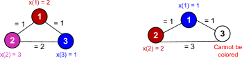
Clearly, Theorem 2 does not apply when the distances are arbitrarily defined. Depending on the edge weights, bipartite graphs may have NO solutions for EQ-CDGP, and graphs which include odd-length cycles may have YES solutions. Figure 11 shows examples of instances considering each case. However, this decision problem can be easily solved for trees, as shown below.

Theorem 3.

Let $G=(V,E,d)$ , be a tree, where $\forall(i,j)\in E\ \ d_{i,j}$ is an arbitrary positive integer. Then $G$ always has a YES solution for EQ-CDGP.

Proof.

We describe a simple algorithm for assigning colors that satisfy the EQ-CDGP problem.

Initially unmark all vertices. Choose an arbitrary vertex $v_{i}$ , assign any positive integer value $x(v_{i})$ to $v_{i}$ , and mark $v_{i}$ . Iteratively, choose an unmarked vertex $v_{j}$ , adjacent to some marked vertex $v_{k}$ . Assign the value $x(v_{j})=d_{jk}+x(v_{j})$ and mark $v_{j}$ . Repeat the iteration until all vertices become marked. ∎

The algorithm described in Theorem 3 has linear time complexity. It is important to note that when this procedure is applied to a MinEQ-CDGP instance, that is, the optimization problem with equality constraints, it only guarantees that a feasible solution is found for a tree, not the optimal one.

4 Algorithmic techniques and methods to solve EQ-CDGP models

In this section, we show some algorithmic strategies to solve our distance geometry graph coloring models, and discuss some algorithmic strategies considering the EQ-CDGP models proposed in the previous section.

4.1 Branch-prune-and-bound methods

For solving the three distance geometry graph coloring models shown in Section 2, we developed three algorithms that combine concepts from constraint propagation and optimization techniques.

A branch-and-prune (BP) algorithm was proposed by Lavor et al. (2012a) for the Discretizable Molecular Distance Geometry Problem (DMDGP), based on a previous version for the MDGP by Liberti et al. (2008). The algorithm proceeds by enumerating possible positions for the vertices that must be located in three-dimensional space ( $\mathbb{R}^{3}$ ), by manipulating the set of available distances. The position for a vertex $i$ , where $i\in[4,n]$ and $n$ is the number of vertices that must be placed in $\mathbb{R}^{3}$ , is determined with respect to the last three vertices that have already been positioned, following the ordering and sphere intersection cited in Section 2. However, a distance between the currently positioned vertex and a previous one that was placed before the last three can be violated, which requires feasibility tests to guarantee that the solution being built is valid. The authors applied the Direct Distance Feasibility (DDF) pruning test, where $\forall(i,j)\in E\ \ |||x(i)-x(j)||-d_{i,j}|<\epsilon$ , and where $\epsilon$ is a given tolerance.

In this work, we adapted these concepts to study and solve our proposed distance geometry coloring models. One of the first reflections that can be made is that for the distance geometry coloring models, there are no initial assumptions to be respected, and thus, there is no explicit vertex ordering to be considered, so we build the ordering by an implicit enumerating process. We mix concepts from branch-and-prune for DMDGP and branch-and-bound procedures to obtain partial solutions (sequences of vertices that have already been colored) that cannot improve on the current best solution.

Our branch-prune-and-bound (BPB) method works as follows. First, a vertex $i$ that has not been colored yet is selected as a starting point. This vertex receives the color $1$ , which is the lowest available (since all colors are positive integers). Then a neighbor $j$ of $i$ that has not been colored yet is selected. A color selection algorithm is used for setting a color to $j$ and the process is repeated recursively for neighbors of $j$ that have not been colored yet. When an uncolored neighbor of the current vertex cannot be found, a uncolored vertex of the graph is used. Pseudocode for this general procedure is given in Algorithm 1.

Algorithm 1 Branch-prune-and-bound general algorithm.

1:graph

G

(with set

V

of vertices and set

E

of edges), function

d:E\rightarrow\mathbb{N}

of distances for each edge, previous vertex

i

, current vertex

j

to be colored, current partial coloring

x

, best complete coloring found

x_{best}

, upper bound

ub

, array

pred

of predecessors from each vertex (initially all set to -1) and enumeration tree depth

dpt

2:function Branch-Prune-And-Bound(

G=(V,E),d,i,j,x,x_{best},ub,pred,dpt

)

3: for each neighbor

k

j

4: if

predec[k]=-1

then

predec[k]\leftarrow i

\triangleright

Set current vertex as predecessor of neighbors

6: if

i=-1

then

i\leftarrow predec[j]

\triangleright

If this call did not come from a neighbor, use predecessor information

colorsAvail\leftarrow

SelectColors(

G,d,i,j,x,ub

)

9: while

colorsAvail\neq\emptyset

10:

color\leftarrow

element of

colorsAvail

11:

colorsAvail\leftarrow colorsAvail-\{color\}

12:

x(j)\leftarrow color

13: if

\max\limits_{v\in V\ |\ v\text{ is colored}}x(v)\geq ub

then

14: Remove color from

i

15: continue

\triangleright

Discard this possible partial solution by bounding

16: if FeasibilityTest(

G,d,f,x,i

) = false then

17: Remove color from

i

18: return

\triangleright

Distance violation, discard partial solution by pruning

19: if

dpt=|V|

then

\triangleright

If true, then all vertices are colored

20: if

\max\limits_{v\in V}x(v)

<

\max\limits_{v\in V}x_{best}(v)

then

21:

x_{best}\leftarrow x

22:

ub\leftarrow\max\limits_{v\in V}x(v)

23: else

24:

hasNeighbor\leftarrow

false

25: for each neighbor

k

j

26: if

k

is not colored then

27:

hasNeighbor\leftarrow

true

28: Branch-Prune-And-Bound(

G,d,f,j,k,x,x_{best},ub,dpt+1

)

29: if

hasNeighbor=

false then

30: for each vertex

k

G

such that

predec[k]\neq-1

\triangleright

Only from vertices with predecessors

31: if

k

is not colored then

32: Branch-Prune-And-Bound(

G,d,f,-1,k,x,x_{best},ub,dpt+1

)

33: Remove color from

i

34: return

x_{best}

We propose different strategies for selecting a color for a vertex and illustrate how the feasibility checking can be done in different levels of the procedure. Each of these cases are discussed below.

Color selection for a vertex

There are two possibilities for determining which colors a vertex can use, determined by the call to SelectColors()), which returns a set of possible colors for a vertex.

The first one, denoted by BPB-Prev, is based on the original BP algorithm by Lavor et al. (2012a). When a vertex $i$ has to be colored, the single previously colored vertex $j$ is taken into account. If $j$ is an invalid vertex, which means that $i$ is not an uncolored neighbor of $j$ , then the only color that $i$ can receive is 1. Otherwise, the function returns a set of cardinality at most 2, whose elements are:

1.

$x(j)+d_{i,j}$ .
2.

$x(j)-d_{i,j}$ (returned only if $x(j)>d_{i,j}$ ).

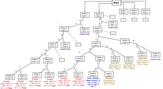
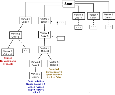
This means that this criterion uses only information from the previous vertex to determine colors, which makes the BPB that uses it an inexact algorithm, something that the original BP for DMDGP also is (Lavor et al., 2012a). However, to counter this in our BPB, when a vertex is colored, its neighbors are marked so that they can use the current vertex as a predecessor in case the search restarts from one of such neighbors. Since we assume the input graph is connected and the algorithm essentially walks through the graph, this information helps to find the true optimal solution. This procedure is done in $O(1)$ time, since only two arithmetic operations are made to determine the colors. An example of this color selection possibility is given in Figure 12.

When using this criterion, we apply the feasibility checking at each colored vertex. However, an alternative is to prune only infeasible solutions where all vertices have colors, that is, we apply the feasibility test only at the last level of the enumeration tree. An example of this alternative is shown in Figure 13, where it is possible to see that this strategy makes the tree grow very large.

The second selection criterion is undertaken using information from all colored neighbors to determine the color for the current vertex $i$ . This is done by solving a system of absolute value inequalities (or equalities, in the case of MinEQ). Those inequalities arise from the distance constraints for the edges. Let $i$ be the vertex that must be colored. The color $x(i)$ must be the solution of a system of absolute value (in)equalities where there is one for each colored neighbor $j$ and each one is as follows:

$|x(j)-x(i)|\ \ \text{OP}\ \ d_{i,j}$

Where OP is either “=” (for MinEQ-CDGP type problems) or “ $\geq$ ” (for MinGEQ-CDGP type problems). The color that will be assigned to $j$ is the smallest value that satisfies all (in)equalities. We note that this procedure always returns a set of cardinality 1, that is, only one color (since only the lowest index is returned) which is also feasible for the partial solution and eventually leads to the optimal solution, although it requires more work per vertex. This selection strategy runs in $O(ub)$ time, where $ub$ is an upper bound for the span, since, to solve the system, we have to mark each possible solution in the interval $[1,ub]$ and select the smallest value. Figure 14 shows an example of an enumeration tree using this color selection strategy.

Feasibility checking

When building a partial solution we must verify if it is feasible when not all distances are taken into account at the same time, especially on BPB-Prev. We used a similar feasibility test to the Direct Distance Feasibility (DDF) used on the BP algorithm for the DMDGP.

Let $i$ be the vertex that has just been colored. Then we must check, for each neighbor $j$ that has already been colored, if the condition $|x(i)-x(j)|\geq d_{i,j}$ (if $f((i,j))=0$ ) or $|x(i)-x(j)|=d_{i,j}$ (if $f((i,j))=1$ ). This test can be seen as a variation of DDF setting $\epsilon$ to zero and allowing inequalities in the test. We denote this procedure as Direct Distance Coloring Feasibility (DDCF) and its pseudocode is given in Algorithm 2.

Algorithm 2 Direct Distance Coloring Feasibility (DDCF) check

1:graph

G

(with set

V

of vertices and set

E

of edges), problem type

t

(MinGEQ-CDGP or MinEQ-CDGP), matrix

d

of distances for each edge, current coloring

x

and vertex

i

2:function DDCF-Check(

G,d,f,x,i

)

3: for each neighbor

k

i

4: if

k

is colored then

5: if

t

= MinGEQ-CDGP then

\triangleright

Inequality constraint

6: if

|x(k)-x(i)|>d_{i,j}

then

7: return false

8: else

\triangleright

Equality constraint

9: if

|x(k)-x(i)|\neq d_{i,j}

then

10: return false

11: return true

We note that when selecting a color using the first criterion (only taking into account the previously colored vertex) the feasibility check can be made at each colored vertex or only when all vertices have been colored (which will require that the function DDF-Check() is called for each vertex). Each check (for only one vertex) runs in $O(|V|)$ time, and if the entire coloring is checked (that is, for all vertices), it runs in $O(|V|^{2})$ time. We also note that, when using the second criterion (using a system of absolute value (in)equalities), the feasibility check can be skipped, since the color that it returns is always feasible.

The combination of these selection criteria and the corresponding feasibility checks result in three possible BPB algorithms, which are summarized in Table 2.

Table 2: Summary of branch-prune-and-bound methods.

Algorithm	Color set size	Color selection of a vertex		Feasibility checking
		Strategy	Time complexity	When	Time complexity
BPB-Prev - Previous neighbor	2	$x(i)=x(j)+d_{i,j}$ or $x(i)=x(j)+d_{i,j}$ (if $x(i)>x(j)+d_{i,j}$ )	$O(1)$	At each colored vertex	$O(\|V\|)$ for each vertex
BPB-Prev-CheckFull - Alternate previous neighbor	2	$x(i)=x(j)+d_{i,j}$ or $x(i)=x(j)+d_{i,j}$ (if $x(i)>x(j)+d_{i,j}$ )	$O(1)$	Only when all vertices are colored	$O(\|V\|^{2})$ for entire coloring
BPB-Select - System of all neighbors	1	$x(i)=\min\{k\in[1,UB]:\forall(i,j)\in E\ \|x(j)-k\|\ =\text{(or $\geq$)}\ d_{i,j}\}$ ,	$O(ub)$	Not needed	-

5 Computational experiments

In order to analyze the behavior of the proposed distance geometry coloring problems and the branch-prune-and-bound algorithms, we made two main sets of experiments: the first one involved generating many random graphs with different numbers of vertices according to some configurations and counting how many include even or odd cycles (while the rest are trees), since some of the properties of distance geometry coloring are related to these types of graphs.

All algorithms used in these experiments were implemented in C language (compiled with gcc 4.8.4 using options -Ofast -march=native -mtune=native) and executed on a computer equipped with an Intel Core i7-3770 (3,4GHz), 8GB of memory and Linux Mint 17 operating system. We describe each set of experiments below.

5.1 Counting members of graph classes in random instances

Using Theorems 2 and 3, we have information about some types of graphs which always have feasible embeddings for EQ-CDGP and EQ-CDGP-Unif. Based on this, we generated a large amount of random graphs with different number of vertices and counted how many were cyclic (and based on that, how many there were for each possibility of having even or odd cycles) and how many were trees.

Each random graph always starts as a random spanning tree, that is, a connected undirected graph $G=(V,E)$ , where $|E|=|V|-1$ . To generate this initial tree, we used a random walk algorithm proposed independently by Broder (1989) and Aldous (1990). The procedure works by using a set $V^{*}$ of the vertices outside the tree and a set $W$ of edges of the spanning tree. Then, whenever the random walk reaches a vertex $j$ outside the tree, the edge $(i,j)$ is added to $E$ and $j$ is removed from $V^{*}$ . This continues until $V^{*}=\varnothing$ . We note that this amounts to making a random walk in a complete graph of $|V|$ vertices and it generates trees in a uniform manner, that is, for all possible spanning trees of a given complete graph, each one has the same probability of being generated by the algorithm.

After the initial tree is generated, we add random new edges to it until the graph has the desired number of edges. This parameter is also randomly set, sampled from interval $\left[|V|-1,\frac{|V|(|V|-1)}{2}\right]$ . This interval ensures that the generated graph is always connected and is, at least, a tree and, at most, a complete graph.

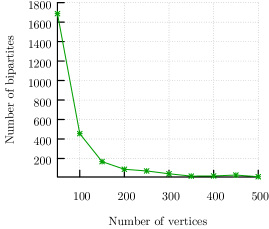
In Table 3, we outline statistics obtained from using the described procedure to generate 1,000,000 (one million) random graphs for each $|V|\in\{50,100,150,200,250,300,350,400,450,500\}$ . As we can observe, most of the graphs (more than 99%) generated have odd cycles, which translates into a very small set of possible EQ-CDGP-Unif instances with feasible embeddings for this configuration of random graphs. By increasing the number of vertices, more possibilities for generating edges appear, but the number of possible connections which will lead to trees or graphs with even cycles is very small. In fact, we can deduce that this configuration generated very few bipartite graphs. For EQ-CDGP (with arbitrary distances), the space of instances with guaranteed feasible embeddings is even smaller, since only trees are certain to have them. However, as shown in Section 3, odd and even cycles can have embeddings depending on how the edges are weighted.

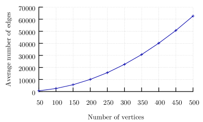
In Figure 15, we can observe the growth of the average number of edges between all generated graphs for each number of vertices. Since the number of edges in a graph is proportional to the square of the number of edges (since $\frac{|V|(|V|-1)}{2}\ \in\ O(|V|^{2})$ , the curve follows a similar pattern, being a half parabola.

Table 3: Number of random graphs with even, odd or no cycles (trees) and bipartite graphs generated for each number of vertices. For each size, 1,000,000 graphs were generated.

$\|V\|$	Average $\|E\|$	Average Density	# Graphs with Odd Cycles	# Graphs with Even Cycles	# Trees	# Bipartite Graphs	CPU Time (sec)
50	637.56	0.5205	998309	854	837	1691	257.07
100	2523.52	0.5098	999553	238	209	447	753.25
150	5656.64	0.5062	999832	74	94	168	1808.25
200	10059.56	0.5055	999910	45	45	90	3403.02
250	15675.94	0.5036	999926	41	33	74	4553.07
300	22586.52	0.5036	999958	18	24	42	6764.28
350	30688.21	0.5025	999975	13	12	25	10042.43
400	40120.76	0.5028	999975	14	11	25	11886.32
450	50678.60	0.5016	999971	15	14	29	14415.33
500	62628.32	0.5020	999988	6	6	12	23332.64

5.2 Results for branch-prune-and-bound algorithms

Table 4: Results for BP algorithm (decision/search) applied to EQ-CDGP instances - 4, 5, 6, 7 and 8 vertices.

			BPB-Prev				BPB-Prev-FeasCheckFull				BPB-Select
$\|$ V $\|$	Type	Inst	Span	# Prunes	# Nodes	CPU Time (s)	Span	# Prunes	# Nodes	CPU Time (s)	Span	# Prunes	# Nodes	CPU Time (s)
4	OddCycle	1	Infeasible	28	36	0.000	Infeasible	36	54	0.000	Infeasible	16	34	0.000
	OddCycle	2	Infeasible	21	32	0.000	Infeasible	25	42	0.000	Infeasible	12	30	0.000
	OddCycle	3	Infeasible	21	32	0.000	Infeasible	22	41	0.000	Infeasible	12	30	0.000
	OddCycle	4	Infeasible	19	32	0.000	Infeasible	21	41	0.000	Infeasible	12	30	0.000
	EvenCycle	1	Infeasible	20	32	0.000	Infeasible	20	32	0.000	Infeasible	8	28	0.000
	EvenCycle	2	Infeasible	20	32	0.000	Infeasible	20	32	0.000	Infeasible	8	28	0.000
	EvenCycle	3	24	0	4	0.000	24	0	4	0.000	24	0	4	0.000
	EvenCycle	4	19	0	4	0.000	19	0	4	0.000	19	0	4	0.000
	Tree	1	21	0	4	0.000	21	0	4	0.000	14	0	4	0.000
	Tree	2	34	0	4	0.000	34	0	4	0.000	14	0	4	0.000
	Tree	3	29	0	4	0.000	29	0	4	0.000	20	0	4	0.000
	Tree	4	41	0	4	0.000	41	0	4	0.000	21	0	4	0.000
5	OddCycle	1	38	0	5	0.000	38	0	5	0.000	38	1	7	0.000
	OddCycle	2	Infeasible	38	58	0.000	Infeasible	56	88	0.000	Infeasible	20	54	0.000
	OddCycle	3	20	1	5	0.000	20	1	6	0.000	20	0	5	0.000
	OddCycle	4	Infeasible	61	69	0.000	Infeasible	106	175	0.000	Infeasible	30	62	0.000
	EvenCycle	1	44	0	5	0.000	44	0	5	0.000	32	1	7	0.000
	EvenCycle	2	36	0	5	0.000	36	0	5	0.000	24	0	5	0.000
	EvenCycle	3	Infeasible	54	77	0.000	Infeasible	66	97	0.000	Infeasible	20	60	0.000
	EvenCycle	4	Infeasible	51	76	0.000	Infeasible	62	96	0.000	Infeasible	20	60	0.000
	Tree	1	20	0	5	0.000	20	0	5	0.000	17	0	5	0.000
	Tree	2	19	0	5	0.000	19	0	5	0.000	19	0	5	0.000
	Tree	3	23	0	5	0.000	23	0	5	0.000	20	0	5	0.000
	Tree	4	39	0	5	0.000	39	0	5	0.000	20	1	7	0.000
6	OddCycle	1	Infeasible	149	161	0.000	Infeasible	378	533	0.001	Infeasible	45	105	0.000
	OddCycle	2	Infeasible	176	168	0.000	Infeasible	887	1114	0.001	Infeasible	76	128	0.000
	OddCycle	3	Infeasible	167	161	0.000	Infeasible	374	465	0.000	Infeasible	48	105	0.000
	OddCycle	4	Infeasible	126	135	0.000	Infeasible	504	624	0.001	Infeasible	43	95	0.000
	EvenCycle	1	Infeasible	100	131	0.000	Infeasible	122	187	0.000	Infeasible	30	97	0.000
	EvenCycle	2	46	0	6	0.000	46	0	6	0.000	21	0	6	0.000
	EvenCycle	3	Infeasible	155	223	0.000	Infeasible	242	381	0.000	Infeasible	60	160	0.000
	EvenCycle	4	Infeasible	84	137	0.000	Infeasible	120	203	0.000	Infeasible	30	100	0.000
	Tree	1	16	0	6	0.000	16	0	6	0.000	13	0	6	0.000
	Tree	2	54	0	6	0.000	54	0	6	0.000	19	0	6	0.000
	Tree	3	34	0	6	0.000	34	0	6	0.000	27	5	17	0.000
	Tree	4	39	0	6	0.000	39	0	6	0.000	39	0	6	0.000
7	OddCycle	1	Infeasible	191	196	0.000	Infeasible	2234	2880	0.003	Infeasible	66	139	0.000
	OddCycle	2	Infeasible	360	307	0.000	Infeasible	5398	6875	0.007	Infeasible	148	229	0.000
	OddCycle	3	Infeasible	383	323	0.000	Infeasible	5360	6506	0.006	Infeasible	138	219	0.000
	OddCycle	4	Infeasible	378	310	0.000	Infeasible	5391	6470	0.006	Infeasible	144	227	0.000
	EvenCycle	1	Infeasible	263	361	0.000	Infeasible	429	686	0.001	Infeasible	91	246	0.000
	EvenCycle	2	36	151	193	0.000	36	192	243	0.000	23	26	105	0.000
	EvenCycle	3	Infeasible	250	283	0.000	Infeasible	1093	1422	0.001	Infeasible	70	178	0.000
	EvenCycle	4	Infeasible	293	382	0.000	Infeasible	511	745	0.001	Infeasible	100	259	0.000
	Tree	1	34	0	7	0.000	34	0	7	0.000	19	0	7	0.000
	Tree	2	33	0	7	0.000	33	0	7	0.000	14	0	7	0.000
	Tree	3	27	0	7	0.000	27	0	7	0.000	27	2	11	0.000
	Tree	4	35	0	7	0.000	35	0	7	0.000	35	1	10	0.000
8	OddCycle	1	Infeasible	650	505	0.001	Infeasible	34796	41815	0.041	Infeasible	220	336	0.000
	OddCycle	2	Infeasible	896	1202	0.001	Infeasible	1750	2191	0.002	Infeasible	145	438	0.000
	OddCycle	3	Infeasible	696	652	0.001	Infeasible	3192	4052	0.004	Infeasible	99	251	0.000
	OddCycle	4	Infeasible	1092	1075	0.001	Infeasible	13940	18078	0.018	Infeasible	311	563	0.001
	EvenCycle	1	51	0	8	0.000	51	0	8	0.000	28	1	10	0.000
	EvenCycle	2	Infeasible	1005	1072	0.001	Infeasible	5410	6544	0.007	Infeasible	230	511	0.000
	EvenCycle	3	Infeasible	1474	1934	0.002	Infeasible	3346	4369	0.005	Infeasible	352	883	0.001
	EvenCycle	4	40	0	8	0.000	40	0	8	0.000	18	4	19	0.000
	Tree	1	45	0	8	0.000	45	0	8	0.000	34	0	8	0.000
	Tree	2	47	0	8	0.000	47	0	8	0.000	29	0	8	0.000
	Tree	3	43	0	8	0.000	43	0	8	0.000	22	0	8	0.000
	Tree	4	71	0	8	0.000	71	0	8	0.000	20	1	10	0.000

Table 5: Results for BP algorithm (decision/search) applied to EQ-CDGP instances - 9, 10, 12, 14 and 16 vertices.

			BPB-Prev				BPB-Prev-FeasCheckFull				BPB-Select
$\|$ V $\|$	Type	Inst	Span	# Prunes	# Nodes	CPU Time (s)	Span	# Prunes	# Nodes	CPU Time (s)	Span	# Prunes	# Nodes	CPU Time (s)
9	OddCycle	1	Infeasible	1638	1537	0.002	Infeasible	46903	60000	0.065	Infeasible	434	777	0.001
	OddCycle	2	Infeasible	1633	1219	0.001	Infeasible	328822	400892	0.397	Infeasible	456	650	0.001
	OddCycle	3	Infeasible	1165	923	0.001	Infeasible	385150	467221	0.456	Infeasible	452	620	0.000
	OddCycle	4	Infeasible	1417	1801	0.002	Infeasible	2479	3574	0.003	Infeasible	297	801	0.001
	EvenCycle	1	61	0	9	0.000	61	0	9	0.000	34	0	9	0.000
	EvenCycle	2	26	0	9	0.000	26	0	9	0.000	20	7	24	0.000
	EvenCycle	3	Infeasible	2011	2542	0.003	Infeasible	3414	4392	0.005	Infeasible	226	788	0.000
	EvenCycle	4	Infeasible	946	1142	0.001	Infeasible	1347	1785	0.002	Infeasible	88	357	0.000
	Tree	1	55	0	9	0.000	55	0	9	0.000	38	10	30	0.000
	Tree	2	68	0	9	0.000	68	0	9	0.000	27	0	9	0.000
	Tree	3	88	0	9	0.000	88	0	9	0.000	29	0	9	0.000
	Tree	4	45	0	9	0.000	45	0	9	0.000	21	0	9	0.000
10	OddCycle	1	Infeasible	33183	42018	0.042	Infeasible	155000	173304	0.168	Infeasible	7939	15821	0.011
	OddCycle	2	Infeasible	2619	1974	0.002	Infeasible	2108251	2797473	2.814	Infeasible	792	1127	0.001
	OddCycle	3	Infeasible	3529	2963	0.003	Infeasible	316389	400670	0.367	Infeasible	710	1184	0.001
	OddCycle	4	Infeasible	4379	3333	0.004	Infeasible	1481970	1818952	1.868	Infeasible	1030	1441	0.001
	EvenCycle	1	Infeasible	3500	3114	0.003	Infeasible	157665	199713	0.174	Infeasible	520	1036	0.001
	EvenCycle	2	Infeasible	46618	48740	0.045	Infeasible	160032	193409	0.224	Infeasible	4718	9984	0.006
	EvenCycle	3	Infeasible	70914	86532	0.086	Infeasible	254208	304707	0.249	Infeasible	4662	10887	0.007
	EvenCycle	4	72	1	10	0.000	72	1	10	0.000	38	0	10	0.000
	Tree	1	59	0	10	0.000	59	0	10	0.000	27	4	18	0.000
	Tree	2	40	0	10	0.000	40	0	10	0.000	31	1	12	0.000
	Tree	3	49	0	10	0.000	49	0	10	0.000	33	4	18	0.000
	Tree	4	46	0	10	0.000	46	0	10	0.000	29	3	16	0.000
12	OddCycle	1	Infeasible	108359	103428	0.115	Infeasible	965368	1140595	1.284	Infeasible	9947	18283	0.012
	OddCycle	2	Infeasible	24433	23227	0.026	Infeasible	1559180	1807872	1.927	Infeasible	1578	3718	0.003
	OddCycle	3	Infeasible	7440	5294	0.006	Infeasible	36724085	44121832	41.883	Infeasible	1426	2058	0.002
	OddCycle	4	Infeasible	8467	5648	0.006	Infeasible	544947529	645413373	390.399	Infeasible	2293	2876	0.002
	EvenCycle	1	49	0	12	0.000	49	0	12	0.000	22	42	146	0.000
	EvenCycle	2	Infeasible	13801	16577	0.017	Infeasible	53860	62497	0.073	Infeasible	954	2799	0.002
	EvenCycle	3	41	0	12	0.000	41	0	12	0.000	35	16	51	0.000
	EvenCycle	4	Infeasible	18820	19828	0.021	Infeasible	381806	495804	0.393	Infeasible	6572	13539	0.009
	Tree	1	38	0	12	0.000	38	0	12	0.000	27	58	139	0.000
	Tree	2	50	0	12	0.000	50	0	12	0.000	22	0	12	0.000
	Tree	3	48	0	12	0.000	48	0	12	0.000	34	440	1016	0.001
	Tree	4	52	0	12	0.000	52	0	12	0.000	26	2	16	0.000
14	OddCycle	1	Infeasible	2725363	2744206	2.820	Infeasible	104517592	118562122	101.605	Infeasible	119828	218219	0.146
	OddCycle	2	Infeasible	34217	23821	0.019	Infeasible	3407171273	4097250986	3314.219	Infeasible	5217	6949	0.005
	OddCycle	3	Infeasible	25749	16751	0.018	Infeasible	11200102605	14120166774	10800.000	Infeasible	4890	6169	0.005
	OddCycle	4	Infeasible	17520	11848	0.013	Infeasible	4872771100	5921495589	5148.447	Infeasible	2844	3883	0.003
	EvenCycle	1	Infeasible	22438	20427	0.022	Infeasible	1726508	1934194	1.889	Infeasible	286	955	0,001
	EvenCycle	2	Infeasible	8815580	9620137	9.640	Infeasible	38618944	42925314	27.755	Infeasible	240185	480564	0.306
	EvenCycle	3	Infeasible	8022290	8013781	7.269	Infeasible	32873088	37749326	29.182	Infeasible	146774	329350	0.205
	EvenCycle	4	Infeasible	4979521	5359288	4.921	Infeasible	16804920	21169856	17.424	Infeasible	160477	354148	0.225
	Tree	1	55	0	14	0.000	55	0	14	0.000	29	54	138	0.000
	Tree	2	63	0	14	0.000	63	0	14	0.000	37	164	385	0.000
	Tree	3	67	0	14	0.000	67	0	14	0.000	31	60	166	0.000
	Tree	4	59	0	14	0.000	59	0	14	0.000	39	647	1432	0.001
16	OddCycle	1	Infeasible	9674081	8970218	8.843	Infeasible	270950088	312103257	218.788	Infeasible	229364	464467	0.295
	OddCycle	2	Infeasible	40827	26130	0.019	Infeasible	9212314467	13585438967	10800.000	Infeasible	10334	12037	0.010
	OddCycle	3	Infeasible	64340	40739	0.031	Infeasible	12857613205	16238297924	10800.000	Infeasible	13417	15677	0.012
	OddCycle	4	Infeasible	79312	71850	0.056	Infeasible	135939959	153954534	104.928	Infeasible	7508	14908	0.010
	EvenCycle	1	79	0	16	0.000	79	0	16	0.000	35	356	799	0.001
	EvenCycle	2	Infeasible	41169779	41680959	35.448	Infeasible	881601120	1035374397	712.612	Infeasible	10410162	19341115	12.607
	EvenCycle	3	72	0	16	0.000	72	0	16	0.000	29	1390	3171	0.002
	EvenCycle	4	Infeasible	61277800	71043803	55.371	Infeasible	250169040	273392839	196.395	Infeasible	787682	1851608	1.155
	Tree	1	65	0	16	0.000	65	0	16	0.000	30	222	502	0.000
	Tree	2	86	0	16	0.000	86	0	16	0.000	30	15	50	0.000
	Tree	3	74	0	16	0.000	74	0	16	0.000	36	329	756	0.001
	Tree	4	79	0	16	0.000	79	0	16	0.000	23	9	42	0.000

Table 6: Results for BP algorithm (decision/search) applied to EQ-CDGP instances - 18 and 20 vertices.

			BPB-Prev				BPB-Prev-FeasCheckFull				BPB-Select
$\|$ V $\|$	Type	Inst	Span	# Prunes	# Nodes	CPU Time (s)	Span	# Prunes	# Nodes	CPU Time (s)	Span	# Prunes	# Nodes	CPU Time (s)
18	OddCycle	1	Infeasible	508400	411189	0.324	Infeasible	14249119873	14806963853	10800.000	Infeasible	18527	33062	0.023
	OddCycle	2	Infeasible	1151865	809413	0.630	Infeasible	6511737586	7859547065	10800.000	Infeasible	29654	46174	0.032
	OddCycle	3	Infeasible	164231	137272	0.093	Infeasible	2830789695	3168256401	3927.393	Infeasible	1411	3456	0.002
	OddCycle	4	Infeasible	117988	72425	0.050	Infeasible	8764779022	9900318687	10800.000	Infeasible	25336	28579	0.022
	EvenCycle	1	Infeasible	11859360	10893632	8.610	Infeasible	1336188416	1468424277	979.763	Infeasible	92766	208614	0.135
	EvenCycle	2	Infeasible	152740084	167194942	127.611	Infeasible	611753448	711245102	598.378	Infeasible	996127	2340311	1.429
	EvenCycle	3	Infeasible	466856235	439993043	298.974	Infeasible	6868230379	7523523165	10800.000	Infeasible	2312073	4373462	2.787
	EvenCycle	4	Infeasible	54784145	53791828	36.624	Infeasible	285915264	360281393	505.807	Infeasible	2527172	5361369	3.354
	Tree	1	88	0	18	0.000	88	0	18	0.000	31	6170	12737	0.008
	Tree	2	61	0	18	0.000	61	0	18	0.000	25	1171	2731	0.002
	Tree	3	91	0	18	0.000	91	0	18	0.000	28	57	157	0.000
	Tree	4	71	0	18	0.000	71	0	18	0.000	30	1634	3433	0.002
20	OddCycle	1	Infeasible	273165199	217944054	169.144	Infeasible	6147895146	9044193773	10800.000	Infeasible	1786324	3216901	2.101
	OddCycle	2	Infeasible	2231047	1503222	1.467	Infeasible	6371122973	8069928711	10800.000	Infeasible	63034	89385	0.066
	OddCycle	3	Infeasible	1049440	744982	0.542	Infeasible	7751043598	8898429750	10800.000	Infeasible	31642	48916	0.035
	OddCycle	4	Infeasible	414762	249339	0.170	Infeasible	13950045871	14504063426	10800.000	Infeasible	56488	64593	0.051
	EvenCycle	1	Infeasible	7618735112	8591239945	7112.081	$ -	-	-	Running	Infeasible	20719998	47209517	29.050
	EvenCycle	2	141	0	20	0.000	141	0	20	0.000	36	13158	25609	0.017
	EvenCycle	3	Infeasible	20754606	17374721	14.777	Infeasible	7684808926	7634511236	10800.000	Infeasible	167148	351029	0.225
	EvenCycle	4	Infeasible	15355600960	14057177765	10800.000	Infeasible	5426010704	7820985965	10800.000	Infeasible	335043320	686615646	428.222
	Tree	1	64	0	20	0.000	64	0	20	0.000	24	107586	201000	0.132
	Tree	2	103	0	20	0.000	103	0	20	0.000	29	560	1443	0.001
	Tree	3	96	0	20	0.000	96	0	20	0.000	36	2908	6536	0.004
	Tree	4	115	0	20	0.000	115	0	20	0.000	27	57601	151814	0.095

In order to use some of the random graphs in experiments with the BPB algorithms, we selected four graphs of each type (with even cycle, with odd cycle and trees) for each number of vertices and randomly weighted the edges with a uniform distribution in the interval $[1,30]$ . We made two subsets of experiments: the first one involved only the EQ-CDGP and EQ-CDGP-Const models, in order to find a feasible solution for each of its instances that were generated (that is, the algorithms use the pruning procedure, but not bounding - equivalently, stopping the search as soon as the first feasible solution is found), and the second one involved the optimization models for each discussed model (MinEQ-CDGP, MinEQ-CDGP-Const, MinGEQ-CDGP and MinGEQ-CDGP-Const).

Tables 4, 5 and 6 give detailed results with 4 to 8, 9 to 16 and 18 to 20 vertices, respectively, considering each BPB algorithm applied to the decision versions. We can see that BPB-Prev reaches a feasible solution faster than the other methods (that is, it solves the decision problem in less time), but it also returns the first feasible solution with a worst span than BPB-Select (noting that BPB-Prev-FeasCheckFull always returns the same span from BPB-Prev because only the pruning point is changed). However, it is much slower to prove that an instance is infeasible (that is, the answer to the decision problem is NO). This is explained by the fact that the enumeration tree is smaller in BPB-Select, since instead of two color possibilities for each vertex, there is only one. Although the time complexity of determining the color for a vertex in BPB-Select is higher (as shown in Table 2), this is compensated by generating a smaller tree and that the feasibility check is not explicitly needed, since it is guaranteed by the color selection algorithm. We also note that BPB-Prev-FeasCheckFull has the worst CPU times for infeasible instances, because the method will keep branching the enumeration tree to find a feasible solution, but since feasibility checking is only done at the leaf nodes, the tree will tend to become the full enumeration tree.

In the same manner, Table 7 shows the results for the BPB algorithms considering the optimization versions and applied only to feasible MinEQ-CDGP instances. For almost all of these instances, BPB-Prev is the best method, BPB-Prev-FeasCheckFull shows similar performance and BPB-Select has worse CPU times. The ties between BPB-Prev and BPB-Prev-FeasCheckFull are explained by the fact that although, in the latter method, the feasibility checking at the leaf nodes increases the time required to find a feasible solution, we keep using the bounding procedures at each node, which reduces the amount of work needed to find the optimal solution. We also note that, for the 4th Tree instance with 20 vertices, BPB-Select does not find the true optimum for the problem. This happens because the method is recursively applied only to vertices which have recorded neighbors, in the same manner as the other two BPBs, but the system of absolute value expressions returns only one color, which may not be the one for the optimal solution when applying the recursion only on some vertices. On some experiments, we detected that, if we generate all vertice orders and apply the color selection of BPB-Select, on them, the optimal solution is found, but the CPU times become very high, since this procedure does not take advantage of the 0-sphere intersection characteristic.

The last experiments were made by applying the BPB algorithms on all instances considered for the algorithms, but by transforming them to MinGEQ-CDGP (changing the $=$ in constraints to $\geq$ ). Since they are always feasible for MinGEQ-CDGP because of its equivalence to BCP, we only have to consider optimization problems, as was already done in Section 2. The same pattern of previous experiments occur here, with BPB-Prev being the best method of the three, however, the CPU time difference between it and BPB-Prev-FeasCheckFull becomes much more apparent here, since there are many more feasible solutions for MinGEQ-CDGP than MinEQ-CDGP.

Table 7: Results for BPB algorithms (optimization) applied to MinEQ-CDGP instances - 4 to 20 vertices.

			BPB-Prev							BPB-Prev-FeasCheckFull							BPB-Select
$\|$ V $\|$	Type	Inst	Span	# Bounds	# Prunes	# Sol.	# Nodes	First Time (s)	Total Time (s)	Span	# Bounds	# Prn.	# Sol.	# Nodes	First Time (s)	Total Time (s)	Span	# Bounds	# Prunes	# Sol.	# Nodes	First Time (s)	Total Time (s)
4	EvenCycle	3	19	12	0	3	26	0.000	0.000	19	12	0	3	26	0.000	0.000	19	8	0	3	25	0.000	0.000
	EvenCycle	4	19	10	0	1	23	0.000	0.000	19	10	0	1	23	0.000	0.000	19	9	0	1	22	0.000	0.000
	Tree	1	14	7	0	3	21	0.000	0.000	14	7	0	3	21	0.000	0.000	14	5	1	1	21	0.000	0.000
	Tree	2	14	6	0	3	21	0.000	0.000	14	6	0	3	21	0.000	0.000	14	5	2	1	24	0.000	0.000
	Tree	3	20	5	0	2	17	0.000	0.000	20	5	0	2	17	0.000	0.000	20	5	2	1	20	0.000	0.000
	Tree	4	21	5	0	2	13	0.000	0.000	21	5	0	2	13	0.000	0.000	21	6	0	1	14	0.000	0.000
5	OddCycle	1	21	24	15	2	57	0.000	0.000	21	24	18	2	67	0.000	0.000	21	16	6	2	50	0.000	0.000
	OddCycle	3	20	24	11	1	52	0.000	0.000	20	28	9	1	63	0.000	0.000	20	18	5	1	50	0.000	0.000
	EvenCycle	1	24	24	0	2	55	0.000	0.000	24	24	0	2	55	0.000	0.000	24	14	8	3	66	0.000	0.000
	EvenCycle	2	19	11	0	4	34	0.000	0.000	19	11	0	4	34	0.000	0.000	19	6	7	2	47	0.000	0.000
	Tree	1	17	32	0	3	64	0.000	0.000	17	32	0	3	64	0.000	0.000	17	15	6	1	58	0.000	0.000
	Tree	2	19	20	0	1	47	0.000	0.000	19	20	0	1	47	0.000	0.000	19	14	3	1	45	0.000	0.000
	Tree	3	20	14	0	2	33	0.000	0.000	20	14	0	2	33	0.000	0.000	20	12	7	1	44	0.000	0.000
	Tree	4	20	8	0	2	26	0.000	0.000	20	8	0	2	26	0.000	0.000	20	10	2	1	32	0.000	0.000
6	EvenCycle	2	21	15	0	4	43	0.000	0.000	21	15	0	4	43	0.000	0.000	21	15	10	1	71	0.000	0.000
	Tree	1	12	19	0	4	46	0.000	0.000	12	19	0	4	46	0.000	0.000	12	13	31	2	111	0.000	0.000
	Tree	2	19	19	0	4	41	0.000	0.000	19	19	0	4	41	0.000	0.000	19	19	23	1	99	0.000	0.000
	Tree	3	19	33	0	4	71	0.000	0.000	19	33	0	4	71	0.000	0.000	19	20	16	2	103	0.000	0.000
	Tree	4	21	30	0	3	64	0.000	0.000	21	30	0	3	64	0.000	0.000	21	18	13	3	85	0.000	0.000
7	EvenCycle	2	23	28	158	2	251	0.000	0.000	23	29	199	2	303	0.000	0.000	23	7	33	1	144	0.000	0.000
	Tree	1	14	29	0	5	72	0.000	0.000	14	29	0	5	72	0.000	0.000	14	18	23	2	139	0.000	0.000
	Tree	2	14	61	0	6	117	0.000	0.000	14	61	0	6	117	0.000	0.000	14	31	25	1	145	0.000	0.000
	Tree	3	16	166	0	6	276	0.000	0.000	16	166	0	6	276	0.000	0.000	16	80	37	2	264	0.000	0.000
	Tree	4	21	154	0	5	277	0.000	0.000	21	154	0	5	277	0.000	0.000	21	73	35	3	240	0.000	0.000
8	EvenCycle	1	21	362	0	9	610	0.000	0.001	21	362	0	9	610	0.000	0.001	21	94	148	4	618	0.000	0.000
	EvenCycle	4	16	158	0	5	320	0.000	0.000	16	158	0	5	320	0.000	0.000	16	110	319	3	1100	0.000	0.001
	Tree	1	26	305	0	6	616	0.000	0.000	26	305	0	6	616	0.000	0.000	26	114	272	2	1055	0.000	0.001
	Tree	2	22	121	0	9	237	0.000	0.000	22	121	0	9	237	0.000	0.000	22	43	116	2	462	0.000	0.000
	Tree	3	18	221	0	6	372	0.000	0.000	18	221	0	6	372	0.000	0.000	18	98	81	2	403	0.000	0.000
	Tree	4	20	66	0	8	119	0.000	0.000	20	66	0	8	119	0.000	0.000	20	50	37	1	219	0.000	0.000
9	EvenCycle	1	22	48	0	5	96	0.000	0.000	22	48	0	5	96	0.000	0.000	22	102	129	2	634	0.000	0.000
	EvenCycle	2	20	7006	0	2	11367	0.000	0.011	20	7006	0	2	11367	0.000	0.012	20	1319	4075	1	11204	0.000	0.007
	Tree	1	24	1078	0	5	1697	0.000	0.001	24	1078	0	5	1697	0.000	0.001	24	363	639	2	2241	0.000	0.001
	Tree	2	27	585	0	6	1067	0.000	0.001	27	585	0	6	1067	0.000	0.001	27	331	1028	1	3181	0.000	0.002
	Tree	3	19	45	0	13	106	0.000	0.000	19	45	0	13	106	0.000	0.000	19	46	66	2	357	0.000	0.000
	Tree	4	19	666	0	6	1012	0.000	0.001	19	666	0	6	1012	0.000	0.001	19	524	1111	2	3778	0.000	0.002
10	EvenCycle	4	26	280	77	8	598	0.000	0.001	26	422	50	8	876	0.000	0.001	26	91	237	3	975	0.000	0.001
	Tree	1	18	256	0	9	346	0.000	0.000	18	256	0	9	346	0.000	0.000	18	305	990	3	2829	0.000	0.002
	Tree	2	26	2112	0	5	3375	0.000	0.003	26	2112	0	5	3375	0.000	0.003	26	1360	5484	3	15417	0.000	0.011
	Tree	3	27	320	0	7	552	0.000	0.000	27	320	0	7	552	0.000	0.001	27	139	738	2	2167	0.000	0.001
	Tree	4	26	881	0	4	1323	0.000	0.001	26	881	0	4	1323	0.000	0.001	26	441	782	3	2884	0.000	0.003
12	EvenCycle	1	19	670	0	9	1361	0.000	0.002	19	670	0	9	1361	0.000	0.001	19	1861	3798	2	14073	0.000	0.008
	EvenCycle	3	29	9332	0	5	15289	0.000	0.017	29	9332	0	5	15289	0.000	0.016	29	2558	18025	2	44790	0.000	0.028
	Tree	1	23	4141	0	4	6440	0.000	0.005	23	4141	0	4	6440	0.000	0.006	23	2045	6647	2	20117	0.000	0.012
	Tree	2	22	4505	0	13	6552	0.000	0.004	22	4505	0	13	6552	0.000	0.005	22	2593	8634	1	23614	0.000	0.014
	Tree	3	22	1301	0	5	2183	0.000	0.002	22	1301	0	5	2183	0.000	0.002	22	850	7513	3	18146	0.001	0.011
	Tree	4	22	857	0	6	1651	0.000	0.002	22	857	0	6	1651	0.000	0.001	22	798	3852	2	12531	0.000	0.010
14	Tree	1	23	38238	0	13	62515	0.000	0.052	23	38238	0	13	62515	0.000	0.056	23	5425	33422	3	88155	0.000	0.054
	Tree	2	23	1007	0	9	2209	0.000	0.002	23	1007	0	9	2209	0.000	0.002	23	3973	24761	2	61087	0.000	0.038
	Tree	3	31	2453	0	6	4429	0.000	0.003	31	2453	0	6	4429	0.000	0.003	31	2965	17661	1	45496	0.000	0.030
	Tree	4	26	54238	0	11	83694	0.000	0.075	26	54238	0	11	83694	0.000	0.080	26	8282	115099	3	269844	0.001	0.163
16	EvenCycle	1	26	182114	0	20	295175	0.000	0.289	26	182114	0	20	295175	0.000	0.198	26	67665	374596	3	965581	0.000	0.583
	EvenCycle	3	26	53810	0	6	98735	0.000	0.077	26	53810	0	6	98735	0.000	0.065	26	21662	87388	2	245263	0.002	0.146
	Tree	1	30	113395	0	10	169791	0.000	0.159	30	113395	0	10	169791	0.000	0.171	30	74842	581089	1	1338678	0.001	0.838
	Tree	2	27	203094	0	22	341417	0.000	0.308	27	203094	0	22	341417	0.000	0.365	27	48245	170534	2	502088	0.000	0.291
	Tree	3	24	3809	0	15	6723	0.000	0.007	24	3809	0	15	6723	0.000	0.007	24	33899	464250	3	1061101	0.000	0.675
	Tree	4	22	1383	0	14	2559	0.000	0.003	22	1383	0	14	2559	0.000	0.003	22	2832	10660	2	43577	0.000	0.024
18	Tree	1	28	8389425	0	25	13361587	0.000	13.669	28	8389425	0	25	13361587	0.000	13.129	28	1999203	5027971	3	13736111	0.008	8.232
	Tree	2	25	496847	0	10	814700	0.000	0.756	25	496847	0	10	814700	0.000	0.895	25	2046711	10251603	1	24302076	0.002	14.682
	Tree	3	23	27147	0	24	45099	0.000	0.037	23	27147	0	24	45099	0.000	0.051	23	106035	1357251	3	3054495	0.000	1.886
	Tree	4	25	17224	0	17	32305	0.000	0.034	25	17224	0	17	32305	0.000	0.034	26	558631	2127000	3	5881291	0.002	3.422
20	EvenCycle	2	24	1916715	0	52	2846521	0.000	2.662	24	1916715	0	52	2846521	0.000	3.759	24	6196691	52250460	5	105240633	0.016	65.083
	Tree	1	24	1128664	0	11	1547952	0.000	1.542	24	1128664	0	11	1547952	0.000	1.466	24	25491780	210995206	1	436478894	0.133	267.977
	Tree	2	27	52049	0	17	87918	0.000	0.099	27	52049	0	17	87918	0.000	0.098	27	417220	2576200	2	6562696	0.001	3.968
	Tree	3	24	176846	0	25	320886	0.000	0.329	24	176846	0	25	320886	0.000	0.325	24	1328968	8067883	3	18762973	0.004	11.476
	Tree	4	26	146052	0	31	217805	0.000	0.124	26	146052	0	31	217805	0.000	0.170	27	72428	4236362	1	10113435	0.082	3.049

Table 8: Results for BPB algorithms (optimization) applied to MinGEQ-CDGP instances - 4 to 10 vertices.

			BPB-Prev							BPB-Prev-FeasCheckFull							BPB-Select
$\|$ V $\|$	Type	Inst	Span	# Bounds	# Prunes	# Sol.	# Nodes	First Time (s)	Total Time (s)	Span	# Bounds	# Prn.	# Sol.	# Nodes	Time 1st (s)	CPU Time (s)	Span	# Bounds	# Prunes	# Sol.	# Nodes	Time to 1st (s)	CPU Time (s)
4	OddCycle	1	34	12	16	2	41	0.000	0.000		12	16	2	47	0.000	0.000	34	2	12	2	40	0.000	0.000
	OddCycle	2	38	10	9	2	31	0.000	0.000	38	11	9	2	35	0.000	0.000	38	6	5	1	30	0.000	0.000
	OddCycle	3	14	11	4	3	29	0.000	0.000	14	14	1	3	32	0.000	0.000	14	3	6	2	30	0.000	0.000
	OddCycle	4	17	13	3	2	31	0.000	0.000	17	16	0	2	34	0.000	0.000	17	3	7	2	32	0.000	0.000
	EvenCycle	1	22	8	3	3	26	0.000	0.000	22	8	3	3	26	0.000	0.000	21	3	4	1	22	0.000	0.000
	EvenCycle	2	19	9	5	3	29	0.000	0.000	19	9	5	3	29	0.000	0.000	19	3	3	2	23	0.000	0.000
	EvenCycle	3	19	12	0	3	26	0.000	0.000	19	12	0	3	26	0.000	0.000	19	8	0	3	25	0.000	0.000
	EvenCycle	4	19	10	0	1	23	0.000	0.000	19	10	0	1	23	0.000	0.000	19	5	4	1	22	0.000	0.000
	Tree	1	14	7	0	3	21	0.000	0.000	14	7	0	3	21	0.000	0.000	14	4	2	1	21	0.000	0.000
	Tree	2	14	6	0	3	21	0.000	0.000	14	6	0	3	21	0.000	0.000	13	3	3	1	20	0.000	0.000
	Tree	3	20	5	0	2	17	0.000	0.000	20	5	0	2	17	0.000	0.000	20	5	2	1	20	0.000	0.000
	Tree	4	21	5	0	2	13	0.000	0.000	21	5	0	2	13	0.000	0.000	21	5	1	1	14	0.000	0.000
5	OddCycle	1	21	24	15	2	57	0.000	0.000	21	24	18	2	67	0.000	0.000	21	14	8	2	49	0.000	0.000
	OddCycle	2	22	16	16	2	51	0.000	0.000	22	18	18	2	61	0.000	0.000	22	10	7	3	57	0.000	0.000
	OddCycle	3	20	24	10	2	53	0.000	0.000	20	28	8	2	63	0.000	0.000	20	12	11	1	50	0.000	0.000
	OddCycle	4	18	26	17	2	65	0.000	0.000	18	50	0	2	95	0.000	0.000	18	9	19	1	71	0.000	0.000
	EvenCycle	1	24	24	0	2	55	0.000	0.000	24	24	0	2	55	0.000	0.000	21	9	9	2	50	0.000	0.000
	EvenCycle	2	19	11	0	4	34	0.000	0.000	19	11	0	4	34	0.000	0.000	15	7	5	2	37	0.000	0.000
	EvenCycle	3	24	17	11	3	52	0.000	0.000	24	18	11	3	57	0.000	0.000	20	9	5	2	40	0.000	0.000
	EvenCycle	4	29	25	12	3	61	0.000	0.000	29	27	12	3	65	0.000	0.000	21	9	8	2	48	0.000	0.000
	Tree	1	17	32	0	3	64	0.000	0.000	17	32	0	3	64	0.000	0.000	17	12	9	1	58	0.000	0.000
	Tree	2	19	20	0	1	47	0.000	0.000	19	20	0	1	47	0.000	0.000	19	9	8	1	47	0.000	0.000
	Tree	3	20	14	0	2	33	0.000	0.000	20	14	0	2	33	0.000	0.000	20	13	6	1	44	0.000	0.000
	Tree	4	20	8	0	2	26	0.000	0.000	20	8	0	2	26	0.000	0.000	20	10	2	1	31	0.000	0.000
6	OddCycle	1	30	75	84	4	205	0.000	0.000	30	120	104	4	344	0.000	0.000	25	9	38	4	137	0.000	0.000
	OddCycle	2	29	125	233	5	358	0.000	0.000	29	212	394	5	783	0.000	0.001	29	11	104	3	297	0.000	0.000
	OddCycle	3	26	72	88	9	189	0.000	0.000	26	100	114	9	293	0.000	0.000	20	11	24	5	102	0.000	0.000
	OddCycle	4	19	48	81	5	150	0.000	0.000	19	70	157	5	276	0.000	0.000	19	13	28	2	109	0.000	0.000
	EvenCycle	1	21	26	11	4	71	0.000	0.000	21	30	7	4	79	0.000	0.000	21	15	12	1	77	0.000	0.000
	EvenCycle	2	21	15	0	4	43	0.000	0.000	21	15	0	4	43	0.000	0.000	21	21	5	1	74	0.000	0.000
	EvenCycle	3	21	54	19	4	126	0.000	0.000	21	63	16	4	149	0.000	0.000	16	31	10	4	116	0.000	0.000
	EvenCycle	4	18	33	9	3	82	0.000	0.000	18	35	10	3	93	0.000	0.000	18	18	10	2	86	0.000	0.000
	Tree	1	12	19	0	4	46	0.000	0.000	12	19	0	4	46	0.000	0.000	12	33	11	2	111	0.000	0.000
	Tree	2	19	19	0	4	41	0.000	0.000	19	19	0	4	41	0.000	0.000	19	29	13	1	99	0.000	0.000
	Tree	3	19	33	0	4	71	0.000	0.000	19	33	0	4	71	0.000	0.000	18	9	18	1	74	0.000	0.000
	Tree	4	21	30	0	3	64	0.000	0.000	21	30	0	3	64	0.000	0.000	21	18	12	2	83	0.000	0.000
7	OddCycle	1	22	101	115	4	249	0.000	0.000	22	288	269	4	763	0.000	0.001	22	35	90	3	289	0.000	0.000
	OddCycle	2	39	349	689	4	927	0.000	0.001	39	920	1860	4	3711	0.000	0.005	39	92	286	1	880	0.000	0.001
	OddCycle	3	26	293	623	11	847	0.000	0.001	26	877	1872	11	3425	0.000	0.004	26	64	249	5	743	0.000	0.001
	OddCycle	4	31	171	526	6	638	0.000	0.001	31	718	2427	6	3872	0.000	0.004	30	31	229	1	584	0.000	0.001
	EvenCycle	1	25	65	44	4	166	0.000	0.000	25	86	37	4	226	0.000	0.000	21	25	34	2	153	0.000	0.000
	EvenCycle	2	23	62	24	5	145	0.000	0.000	23	63	27	5	150	0.000	0.000	21	32	16	2	147	0.000	0.000
	EvenCycle	3	24	89	54	6	203	0.000	0.000	24	156	79	6	359	0.000	0.000	21	37	21	3	164	0.000	0.000
	EvenCycle	4	18	50	12	4	105	0.000	0.000	18	60	8	4	124	0.000	0.000	18	37	27	1	155	0.000	0.000
	Tree	1	14	29	0	5	72	0.000	0.000	14	29	0	5	72	0.000	0.000	13	21	8	3	98	0.000	0.000
	Tree	2	14	61	0	6	117	0.000	0.000	14	61	0	6	117	0.000	0.000	14	27	33	3	184	0.000	0.000
	Tree	3	16	166	0	6	276	0.000	0.000	16	166	0	6	276	0.000	0.000	16	92	53	2	356	0.000	0.000
	Tree	4	21	154	0	5	277	0.000	0.000	21	154	0	5	277	0.000	0.000	21	96	39	3	320	0.000	0.000
8	OddCycle	1	$ -	-	-	-	-	-	Running	49	3564	20774	10	29653	0.000	0.035	49	333	1086	3	3454	0.000	0.003
	OddCycle	2	24	183	64	4	422	0.000	0.001	24	191	104	4	481	0.000	0.001	24	52	130	1	516	0.000	0.000
	OddCycle	3	20	244	168	3	573	0.000	0.001	20	459	201	3	1035	0.000	0.001	20	40	100	4	400	0.000	0.000
	OddCycle	4	18	409	235	4	855	0.000	0.001	18	905	980	4	2672	0.000	0.003	18	279	106	3	808	0.000	0.001
	EvenCycle	1	$ -	-	-	-	-	-	Running	21	362	0	9	610	0.000	0.001	16	136	60	3	460	0.000	0.000
	EvenCycle	2	20	207	257	8	550	0.000	0.001	20	285	594	8	1156	0.000	0.001	20	94	90	3	412	0.000	0.000
	EvenCycle	3	20	278	312	11	778	0.000	0.001	20	373	402	11	1113	0.000	0.001	19	82	100	2	442	0.000	0.000
	EvenCycle	4	16	158	0	5	320	0.000	0.000	16	158	0	5	320	0.000	0.000	15	332	46	4	857	0.000	0.001
	Tree	1	26	305	0	6	616	0.000	0.001	26	305	0	6	616	0.000	0.001	21	115	113	3	584	0.000	0.000
	Tree	2	22	121	0	9	237	0.000	0.000	22	121	0	9	237	0.000	0.000	18	90	51	2	390	0.000	0.000
	Tree	3	18	221	0	6	372	0.000	0.000	18	221	0	6	372	0.000	0.000	18	125	133	2	679	0.000	0.000
	Tree	4	20	66	0	8	119	0.000	0.000	20	66	0	8	119	0.000	0.000	20	40	64	2	290	0.000	0.000
9	OddCycle	1	34	1094	2322	6	3890	0.000	0.004	34	4304	12208	6	22898	0.001	0.026	34	149	984	5	2793	0.000	0.002
	OddCycle	2	40	3370	8078	8	8822	0.000	0.011	40	39699	110777	8	190479	0.000	0.228	34	465	2638	5	5960	0.000	0.005
	OddCycle	3	31	2771	12854	14	14713	0.000	0.018	31	25017	216547	14	299935	0.007	0.364	31	1123	4532	2	12065	0.000	0.010
	OddCycle	4	31	192	73	6	426	0.000	0.001	31	252	82	6	567	0.000	0.001	21	87	81	4	393	0.000	0.000
	EvenCycle	1	22	48	0	5	96	0.000	0.000	22	48	0	5	96	0.000	0.000	21	64	120	2	485	0.000	0.000
	EvenCycle	2	20	7006	0	2	11367	0.000	0.013	20	7006	0	2	11367	0.000	0.013	16	2564	701	1	6564	0.000	0.004
	EvenCycle	3	22	163	31	10	318	0.000	0.000	22	179	30	10	353	0.000	0.000	21	43	78	2	374	0.000	0.000
	EvenCycle	4	19	86	25	6	210	0.000	0.000	19	103	12	6	238	0.000	0.000	18	17	33	1	165	0.000	0.000
	Tree	1	24	1078	0	5	1697	0.000	0.002	24	1078	0	5	1697	0.000	0.002	21	217	216	3	912	0.000	0.001
	Tree	2	27	585	0	6	1067	0.000	0.001	27	585	0	6	1067	0.000	0.001	21	354	356	1	1492	0.000	0.001
	Tree	3	19	45	0	13	106	0.000	0.000	19	45	0	13	106	0.000	0.000	18	56	38	3	276	0.000	0.000
	Tree	4	19	666	0	6	1012	0.000	0.001	19	666	0	6	1012	0.000	0.001	16	172	657	2	1754	0.000	0.001
10	OddCycle	1	35	3003	7975	10	14123	0.000	0.018	35	9709	26544	10	43331	0.000	0.055	35	4458	5347	3	21621	0.000	0.017
	OddCycle	2	28	6667	16959	10	19750	0.000	0.024	28	223072	400955	10	906517	0.011	1.125	27	1329	10080	6	22206	0.000	0.017
	OddCycle	3	29	2823	8230	10	10695	0.000	0.014	29	24168	77732	10	136667	0.000	0.172	29	766	2592	4	7877	0.000	0.006
	OddCycle	4	34	5561	12524	9	15171	0.000	0.019	34	96871	286890	9	487391	0.000	0.607	34	702	8012	5	16534	0.000	0.014
	EvenCycle	1	20	3134	2760	10	7361	0.001	0.009	20	13435	9751	10	34744	0.004	0.041	20	247	1057	3	2947	0.000	0.002
	EvenCycle	2	17	4576	1461	9	8398	0.000	0.011	17	7008	60	9	11364	0.000	0.014	17	1626	2065	3	8519	0.000	0.006
	EvenCycle	3	22	1877	266	3	2902	0.000	0.003	22	3584	0	3	5266	0.000	0.006	21	846	894	2	3697	0.000	0.003
	EvenCycle	4	25	291	56	9	598	0.000	0.001	25	393	39	9	787	0.000	0.001	20	47	39	3	218	0.000	0.000
	Tree	1	18	256	0	9	346	0.000	0.000	18	256	0	9	346	0.000	0.000	18	590	783	2	2958	0.000	0.002
	Tree	2	26	2112	0	5	3375	0.000	0.004	26	2112	0	5	3375	0.000	0.004	20	446	141	3	1127	0.000	0.001
	Tree	3	27	320	0	7	552	0.000	0.001	27	320	0	7	552	0.000	0.001	21	156	360	3	1244	0.000	0.001
	Tree	4	26	881	0	4	1323	0.000	0.002	26	881	0	4	1323	0.000	0.002	20	598	291	3	2005	0.000	0.001

Table 9: Results for BPB algorithms (optimization) applied to MinEQ-CDGP instances - 12 to 20 vertices.

			BPB-Prev							BPB-Prev-FeasCheckFull							BPB-Select
$\|$ V $\|$	Type	Inst	Span	# Bounds	# Prunes	# Sol.	# Nodes	First Time (s)	Total Time (s)	Span	# Bounds	# Prn.	# Sol.	# Nodes	Time 1st (s)	CPU Time (s)	Span	# Bounds	# Prunes	# Sol.	# Nodes	Time to 1st (s)	CPU Time (s)
18	OddCycle	1	24	128682	169800	36	303312	0.000	0.331	24	57939861	55723668	36	147688713	0.011	181.333	23	89251	2157123	6	4215186	0.000	3.294
	OddCycle	2	28	195913	344857	21	481728	0.000	0.685	28	171250440	166458915	21	447646216	0.009	503.647	28	156374	725207	10	1786184	0.000	1.283
	OddCycle	3	29	52772	52858	26	116964	0.000	0.146	29	3292370	2066685	26	7598024	0.000	8.484	27	28930	127942	4	383073	0.000	0.298
	OddCycle	4	57	765800493	2410439059	44	1844704597	0.000	2165.522	84	388902913	8179300886	26	9777141840	0.000	10800.000	56	254968496	7563812423	15	11912285919	0.000	10800.000
	EvenCycle	1	22	36813	17943	43	69147	0.000	0.056	22	341699	9988	43	539430	0.000	0.533	21	153559	261663	6	929927	0.000	0.539
	EvenCycle	2	27	299602	61969	23	533097	0.000	0.739	27	546904	11706	23	911089	0.000	1.095	21	441889	1561547	4	5096657	0.000	3.778
	EvenCycle	3	26	1086457	1493813	17	2963076	0.000	3.927	26	12126525	7756606	17	28907005	0.033	32.674	21	2328257	2049088	3	8815279	0.000	6.128
	EvenCycle	4	21	75255	14380	12	148619	0.000	0.181	21	178965	25836	12	368870	0.000	0.399	17	54179	692407	5	1749663	0.000	1.318
	Tree	1	28	8389425	0	25	13361587	0.000	18.072	28	8389425	0	25	13361587	0.000	16.323	21	3480825	11725139	5	31510553	0.000	24.106
	Tree	2	25	496847	0	10	814700	0.000	1.140	25	496847	0	10	814700	0.000	0.871	21	3385503	5562843	3	16351954	0.000	11.111
	Tree	3	23	27147	0	24	45099	0.000	0.061	23	27147	0	24	45099	0.000	0.048	19	1168701	3161985	2	10148322	0.000	7.577
	Tree	4	25	17224	0	17	32305	0.000	0.035	25	17224	0	17	32305	0.000	0.036	21	3617491	3960687	4	17214598	0.000	11.342
20	OddCycle	1	25	22163660	22312193	29	48128543	0.000	52.703	25	1098477035	898689359	29	2635612691	0.000	2834.168	25	30005823	182202237	2	481689865	0.000	298.143
	OddCycle	2	30	18199655	57912028	24	62598812	0.000	59.472	33	1384131561	6610913025	21	10548373532	0.005	10800.000	30	9486329	105756952	5	248377444	0.000	170.801
	OddCycle	3	30	4723994	12256692	33	14889051	0.000	15.432	37	1313725187	7755384023	28	11169891551	0.000	10800.000	29	3280215	14139380	4	35525456	0.000	24.019
	OddCycle	4	51	1326464513	4631500220	44	3584556973	0.000	3810.559	73	638518954	9954255379	31	11074870144	0.000	10800.000	50	367727937	7605396821	14	12755365765	0.000	10800.000
	EvenCycle	1	24	7208896	2212099	19	14803299	0.000	16.686	24	10219092	8719552	19	29371082	0.000	32.160	21	244902785	91113414	5	724708042	0.000	418.513
	EvenCycle	2	24	1916715	0	52	2846521	0.000	3.037	24	1916715	0	52	2846521	0.000	3.078	21	265125525	35429733	2	548890756	0.000	316.485
	EvenCycle	3	26	417941	457800	31	935063	0.000	0.942	26	17707200	18010642	31	45679688	0.000	43.227	21	4529934	1546737	5	12937093	0.000	8.702
	EvenCycle	4	26	215044982	697065560	17	1421952015	846.276	1415.138	26	919810062	5667438936	17	9537061616	6903.557	9588.792	21	266995348	272027469	2	1143758266	0.000	680.188
	Tree	1	24	1128664	0	11	1547952	0.000	1.684	24	1128664	0	11	1547952	0.000	1.796	21	497365528	932560094	5	3285799702	0.000	1977.674
	Tree	2	27	52049	0	17	87918	0.000	0.089	27	52049	0	17	87918	0.000	0.087	21	27313206	17555281	4	98225542	0.000	61.035
	Tree	3	24	176846	0	25	320886	0.000	0.356	24	176846	0	25	320886	0.000	0.249	21	11863544	18549550	4	65387940	0.000	42.189
	Tree	4	26	146052	0	31	217805	0.000	0.249	26	146052	0	31	217805	0.000	0.176	21	8637029	3463966	3	21799871	0.000	13.998

6 Concluding remarks

In this paper, we proposed some distance geometry models for graph coloring problems with distance constraints that can be applied to important, modern real world applications, such as in telecommunications for channel assignment in wireless networks. In these proposed coloring distance geometry problems (CDGPs), the vertices of the graph are embedded on the real line and the coloring is treated as an assignment of natural numbers to the vertices, while the distances correspond to line segments, whose objective is to determine a feasible intersection of them.

We tackle such problems under the graph theory approach, to establish conditions of feasibility through behavior analysis of the problems in certain classes of graphs, identifying prohibited structures for which the occurrence indicates that it can not admit a valid solution, as well as identifying classes graphs that always admit valid solution.

We also developed exact and approximate enumeration algorithms, based on the Branch-and-Prune (BP) algorithm proposed for the Discretizable Molecular Distance Geometry Problem (DMDGP), combining concepts from constraint propagation and optimization techniques, resulting in Branch-Prune-and-Bound algorithms (BPB), that handle the set of distances in different ways in order to get feasible and optimal solutions. The computational experiments involved equality and inequality constraints and both uniform and arbitrary sets of distances, where we measure the number of prunes and bounds and the CPU time needed to reach the best solution.

Ongoing and future works include improving the BPB formulations by domain reduction and more specific constraints; developing hybrid methods, involving integer and constraint programming; and applying heuristics, in order to solve the proposed distance coloring models more efficiently. Studying problems posed to specific classes of graphs, in order to establish other characterizations of feasibility conditions for more general CDGP problems, is also a subject of research in progress.

Acknowledgement

We would like to thank Dr. Leo Liberti, professor at LIX - École Polytechnique, France, for his valuable contribution to this work, having identified a relationship between coloring problems in graphs with additional constraints on the edges and distance geometry problems, and for discussing some of the ideas presented here.

References

Akihiro et al. (2002) U. Akihiro, I. Hiro, U. Hideyuki, and Y. Mitsuo. A Coloring Problem With Restrictions of Adjacent Colors. International Transactions in Operational Research, 9(2):183–194, 2002. doi: 10.1111/1475-3995.00349.
Aldous (1990) D. Aldous. The random walk construction of uniform spanning trees and uniform labelled trees. SIAM Journal on Discrete Mathematics, 3(4):450–465, 1990.
Audhya et al. (2011) G. Audhya, K. Sinha, S. Ghosh, and B. Sinha. A survey on the channel assignment problem in wireless networks. Wireless Communications and Mobile Computing, 11:583–609, 2011.
Bondy and Murty (2008) J. Bondy and U. Murty. Graph Theory: Graduate Texts in Mathematics. Springer, 3rd edition, 2008.
Broder (1989) A. Broder. Generating random spanning trees. In 30th Annual Symposium on Foundations of Computer Science, pages 442–447. IEEE, 1989.
Dias (2014) B. Dias. Theoretical models and algorithms for optimizing channel assignment in wireless mobile networks. Master’s thesis, Federal University of Amazonas, Brazil, 2014. In portuguese.
Dias et al. (2012) B. Dias, R. Freitas, and N. Maculan. Alocação de canais em redes celulares sem fio: algoritmos e modelos teóricos em grafos e escalonamento. In Proceedings of the XVI Latin-Ibero-American Conference on Operations Research / XLIV Brazilian Symposium of Operations Research. Brazilian Society of Operations Research (SOBRAPO), 2012. In portuguese.
Dias et al. (2013) B. Dias, R. Freitas, and J. Szwarcfiter. On graph coloring problems with distance constraints. In Proceedings of I Workshop on Distance Geometry and Applications (DGA 2013), 2013.
Freitas et al. (2014a) R. Freitas, B. Dias, N. Maculan, and J. Szwarcfiter. On feasibility conditions in graph coloring problems with distance constraints. In Many Faces of Distances (Workshop), 2014a.
Freitas et al. (2014b) R. Freitas, C. Santos, B. Dias, C. Lavor, N. Maculan, and J. Szwarcfiter. Some notes on Euclidean distance geometry and graph theory involving telecom, computer networks and molecular biology applications. In 20th Conference of the International Federation of Operational Research Societies (IFORS 2014), 2014b.
Garey and Johnson (1979) M. Garey and D. Johnson. Computers and Intractability: A Guide to the Theory of NP-Completeness. W. H. Freeman, 1979.
Hale (1980) W. Hale. Frequency assignment: Theory and applications. Proceedings of the IEEE, 25:1497–1514, 1980.
Karp (1972) Richard Karp. Reducibility Among Combinatorial Problems. In R. E. Miller and J. W. Thatcher, editors, Complexity of Computer Computations, pages 85–103. Plenum Press, 1972.
Koster (1999) A. Koster. Frequency assignment: models and algorithms. PhD thesis, Universiteit Maastricht, the Netherlands, 1999.
Koster and Munhoz (2010) A. Koster and X. Munhoz. Graphs and Algorithms in Communication Networks: Studies in Broadband, Optical, Wireless and Ad Hoc Networks. Texts in Theoretical Computer Science. Springer, 2010.
Lavor et al. (2012a) C. Lavor, L. Liberti, N. Maculan, and A. Mucherino. The discretizable molecular distance geometry problem. European Journal of Operational Research, 52(1):115–146, 2012a.
Lavor et al. (2012b) C. Lavor, L. Liberti, N. Maculan, and A. Mucherino. Recent advances on the discretizable molecular distance geometry problem. Computational Optimization and Applications, 219(3):698–706, 2012b.
Liberti et al. (2008) L. Liberti, C. Lavor, and N. Maculan. A branch-and-prune algorithm for the molecular distance geometry problem. International Transactions in Operational Research, 15(1):1–17, 2008.
Liberti et al. (2014) L. Liberti, C. Lavor, N. Maculan, and A. Mucherino. Euclidean Distance Geometry and Applications. SIAM Review, 56(1):3–69, 2014.
Malaguti and Toth (2010) E. Malaguti and P. Toth. A survey on vertex coloring problems. International Transactions in Operational Research, 17(1):1–34, 2010. doi: 10.1111/j.1475-3995.2009.00696.x.
Mucherino et al. (2013) A. Mucherino, C. Lavor, L. Liberti, and N. Maculan. Distance Geometry: Theory, Methods and Applications. Springer, 2013.
Saxe (1979) J. B. Saxe. Embeddability of weighted graphs in $k$ -space is strongly NP-hard. In Proceedings of 17th Allerton Conference in Communications, Control and Computing, pages 480–489, 1979.