Topological Magnon Bands in Ferromagnetic Star Lattice

Abstract

The experimental observation of topological magnon bands and thermal Hall effect in a kagomé lattice ferromagnet Cu(1-3, bdc) has inspired the search for topological magnon effects in various insulating ferromagnets that lack an inversion center allowing a Dzyaloshinskii-Moriya (DM) spin-orbit interaction. The star lattice (also known as the decorated honeycomb lattice) ferromagnets is an ideal candidate for this purpose because it is a variant of the kagomé lattice with additional links that connect the up-pointing and down-pointing triangles. This gives rise to twice the unit cell of the kagomé lattice, hence a more interesting topological magnon effects. In particular, the triangular bridges on the star lattice can be coupled either ferromagnetically or antiferromagnetically which is not possible on the kagome lattice ferromagnets. Here, we study DM-induced topological magnon bands, chiral edge modes, and thermal magnon Hall effect on the star lattice ferromagnet in different parameter regimes. The star lattice can also be visualized as the parent material from which topological magnon bands can be realized for the kagomé and honeycomb lattices in some limiting cases.

I Introduction

Topological magnon matter is the magnonic analog of topological fermionic matter. In contrast, magnons are charge-neutral bosonic excitations of ordered quantum magnets. Thus, the transport properties of magnons are believed to be the new direction for dissipationless transports in insulating ferromagnets applicable to modern technology such as magnon spintronics and magnon thermal devices kru ; kru1 ; kru2 . In insulating collinear quantum magnets the DM interaction dm ; dm1 arising from spin-orbit coupling (SOC) dm1 is the key ingredient that leads to thermal magnon Hall effect alex0 ; alex1 ; alex1a ; alex6 and topological magnon bands alex2 ; alex7 ; alex6a ; hir ; shin ; shin1 ; zhh ; alex4a ; alex4 ; jh ; sol ; sol1 ; kkim . The DM interaction is present in magnetic systems that lack inversion symmetry between magnetic ions. The kagomé lattice is built with this structure, because the midpoint of the bonds connecting two nearest-neighbour magnetic ions is not a center of inversion. Therefore, a DM interaction is intrinsic to the kagomé lattice. The thermal magnon Hall effect induced by the DM interaction was first observed experimentally in a number of three-dimensional (3D) ferromagnetic pyrochlores — Lu₂V₂O₇, Ho₂V₂O₇, and In₂Mn₂O₇ alex1 ; alex1a . Subsequently, the thermal magnon Hall effect was realized in a kagomé ferromagnet Cu(1-3, bdc) alex6 followed by the first experimental realization of topological magnon bands alex6a in the same material. On the other hand, no topologcal magnon bands have been observed in pyrochlore ferromagnets, but recent studies have proposed Weyl magnons in 3D pyrochlore ferromagnets mok ; su .

In the same way a pyrochlore lattice can be visualized as an alternating kagomé and triangular layers, the star lattice (also known as the decorated honeycomb lattice) can be visualized as an interpolating lattice between the honeycomb lattice and the kagomé lattice. The number of sites per unit cell in star lattice is six, three times as in honeycomb and twice as in kagome. Most importantly, the star lattice plays a prominent role in different branches of physics. The Kitaev model on the star lattice has an exact solution as a chiral spin liquid zheng1 . The star lattice also plays an important role in ultracold atoms zheng6 . In particular, quantum magnets zheng ; zheng1 ; zheng3 ; zheng4 ; zheng6 and topological insulators zheng2 ; zheng5 ; zheng5a on the star-lattice show distinctive remarkable features different from the kagome and honeycomb lattices.

Motivated by these interesting features on the star lattice, the study of topological magnon bands on the star lattice is necessary and unavoidable. In this work, we study the topological magnon bands and the thermal magnon Hall response in insulating quantum ferromagnet on the star lattice. We show that lack of an inversion center allows a DM interaction between the midpoint of the triangular bonds. The DM interaction induces a fictitious magnetic flux in the unit cell and leads to nontrivial topological magnon bands. This directly leads to the existence of nonzero Berry curvatures and Chern numbers accompanied by topologically protected gapless edge modes. Indeed, it is feasible to synthesize magnetic materials with the star structure and directly confirm the present theoretical results.

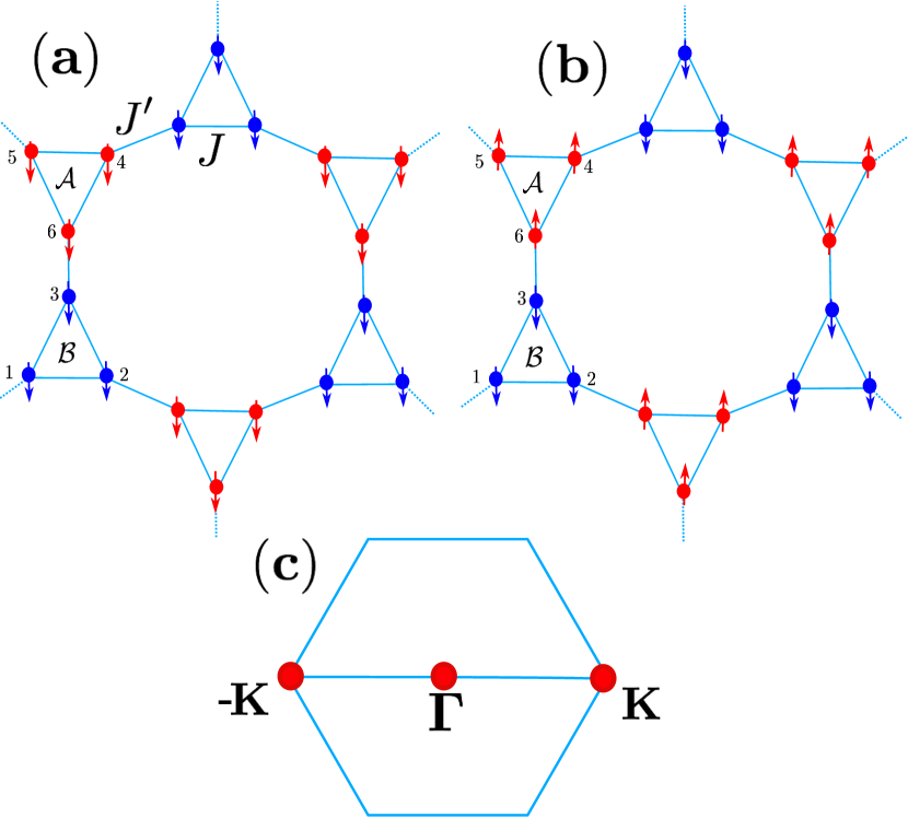
Figure 1: Color online. Schematics of star lattice. (a) Coupled ferromagnets within and between triangles of the star lattice. (b) Coupled antiferromagnets between the triangles. (c). The Brillouin zone of the star lattice.

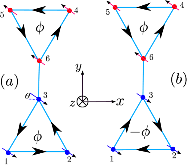
Figure 2: The possible configurations of the DM-induced flux $\phi_{ij}$ (see Appendix A) in the presence of a magnetic field, where $\theta$ is the field-induced canting angle. Bold arrows indicate the sign of the fictitious magnetic flux $\phi_{ij}$ and the small arrows show the magnetic-field-induced spin canting in the $x$-$z$ plane. $(a)$ Uniform flux. $(b)$ Staggered flux.

II Ferromagnetic Hamiltonian

Quantum magnets on the star lattice are known to possess magnetic long-range orders zheng ; zheng4 . However, the effects of the intrinsic DM perturbation have not been considered on the star lattice. Here, we study a ferromagnetic model which is a magnetically ordered state on the star lattice. The Hamiltonian is given by

$$\mathcal{H} =\mathcal{H}_{0}+\mathcal{H}_{Z}+\mathcal{H}_{\text{pert}},$$ (1)

where

$$\mathcal{H}_{0}=-J\sum_{\langle ij\rangle}{\bf S}_{i}\cdot{\bf S}_{j}+J^{\prime}\sum_{\langle ij\rangle}{\bf S}_{i}\cdot{\bf S}_{j},$$ (2)

and $J,J^{\prime}$ are exchange couplings within sites on the triangles “$\Delta$” and between triangles “$\Delta\leftrightarrow\nabla$” as shown in Fig. 1. The Zeeman magnetic field is given by

$$\mathcal{H}_{Z}=-\mathbb{H}\cdot\sum_{i}{\bf S}_{i},$$ (3)

where $\mathbb{H}=h\mathbb{\hat{z}}$ with $h=g\mu_{B}H$ is the strength of the out-of-plane magnetic field. The last term $\mathcal{H}_{\text{pert}}$ represents all the perturbative interactions to the Heisenberg exchange. The DM interaction is usually the dominant perturbative anisotropy. It is allowed on the star-lattice due to lack of inversion center between magnetic ions according to the Moriya rule dm1 . The magneto-crystalline anisotropy is second order in perturbation which can be neglected. Therefore, we will consider only the DM perturbation term. Hence,

$$\mathcal{H}_{\text{pert}}=\sum_{\langle ij\rangle}\mathbb{D}_{ij}\cdot{\bf S}_{i}\times{\bf S}_{j}.$$ (4)

There are two ferromagnetic ordered states on the star-lattice. The first one corresponds to $J>0$ and $J^{\prime}<0$, i.e. fully polarized ferromagnets on sublattice $\mathcal{A}$ (down pointing triangles indicated with blue sites) and $\mathcal{B}$ (up pointing triangles indicated with red sites) as shown in Fig. 1. The second one corresponds to $J>0$ and $J^{\prime}>0$, i.e., antiferromagnetic interaction between triangles and ferromagnetic interaction on each triangle. In the latter case the spins on sublattice $\mathcal{A}$ are oriented in the opposite direction to those on sublattice $\mathcal{B}$, and they also cant along the magnetic field direction as shown in Fig. 2. As we will show in the subsequent sections, the latter case recovers the former case at the saturation field $h_{s}=2J^{\prime}S$.

III Results

III.1 Ground state energy

At zero field the spins are aligned along the star plane chosen as the $x$-$y$ plane with the quantization axis chosen along the $x$-direction. The ground state is a collinear ferromagnet unaffected by the DM interaction. However, if the sublattices $\mathcal{A}$ and $\mathcal{B}$ are coupled antiferromagnetically, that is $J>0$ and $J^{\prime}>0$, then a small magnetic field induces canting along the direction of the field and the ground state is no longer the collinear ferromagnets. The collinear ferromagnet is only recovered at the saturation field $h_{s}$. In the large-$S$ limit, the spin operators can be approximated as classical vectors, written as $\mathbb{S}_{\tau}=S\mathbb{n}_{\tau}$, where $\mathbb{n}_{\tau}=\left(\sin\theta\cos\vartheta_{\tau},\sin\theta\sin\vartheta_{\tau},\cos\theta\right)$ is a unit vector and $\tau$ denotes the down ($\mathcal{A}$) and up ($\mathcal{B}$) triangles, with $\vartheta_{\mathcal{A}}=0$ and $\vartheta_{\mathcal{B}}=\pi$ and $\theta$ is the magnetic-field-induced canting angle. As the system is ordered ferromagnetically on each triangle, the DM interaction does not contribute to the classical energy given by

$$e_{0}=-JS^{2}+\frac{J^{\prime}S^{2}}{2}\cos 2\theta-hS\cos\theta,$$ (5)

where $e_{0}=E/6N$ is energy per site and $N$ is the number of sites per unit cell. Minimizing the classical energy yields the canting angle $\cos\theta=h/h_{s}$.

III.2 Magnetic excitations

In the low temperature regime the magnetic excitations above the classical ground state are magnons and higher order magnon-magnon interactions are negligible. Thus, the linearized Holstein-Primakoff (HP) spin-boson representation HP is valid. Due to the magnetic-field-induced spin canting, we have to rotate the coordinate axes such that the $z$-axis coincides with the local direction of the classical polarization. This involves rotating the spins from laboratory frame to local frame by the spin oriented angles $\vartheta_{\tau}$ about the $z$-axis. This rotation is followed by another rotation about the $y$-axis with the canting angle $\theta$, and the resulting transformation is given by

$$S_{i\tau}^{x}=\pm S_{i\tau}^{\prime x}\cos\theta\pm S_{i\tau}^{\prime z}\sin\theta,$$

$$S_{i\tau}^{y}=\pm S_{i\tau}^{\prime y},$$ (6)

$$S_{i\tau}^{z}=-S_{i\tau}^{\prime x}\sin\theta+S_{i\tau}^{\prime z}\cos\theta,$$

where $+(-)$ applies to the spins residing on the sublattice $\mathcal{A}$ ($\mathcal{B}$) triangles respectively. It is easily checked that this rotation does not affect the collinear ferromagnetic ordering on each triangle, that is the $J$ term.

Usually, in collinear ferromagnets the perpendicular-to-field DM component does to contribute to the free magnon theory because the magnetic moments are polarized along the magnetic field direction alex1 ; alex1a ; alex6 . Therefore, only the parallel-to-field DM component has a significant contribution to the free magnon dispersion alex2 ; alex7 ; alex6a ; hir ; shin ; shin1 ; zhh ; alex4a ; alex4 ; jh ; sol ; sol1 ; kkim ; alex0 ; alex1 ; alex1a ; alex6 . In the present model, however, the situation is different. Due to antiferromagnetic coupling between triangles an applied magnetic field induces two spin components — one parallel to the field and the other perpendicular to the field. As we pointed out above, the DM interaction has a finite contribution to the free magnon model only when the magnetic moments are along its direction. Therefore the parallel-to-field DM component (${\bf D}\parallel{\bf H}$) and the perpendicular-to-field DM component (${\bf D}\perp{\mathbb{H}}$) will have a finite contribution to the free magnon theory due to spin canting. The former is rescaled as $D_{\parallel,\theta}\to D\cos\theta$ and the latter is rescaled as $D_{\perp,\theta}\to D\sin\theta$ by the magnetic field. Implementing the spin transformation (III.2) the terms that contribute to the free magnon model are given by

$$\mathcal{H}_{0}=-J\sum_{\langle i,j\rangle\tau}{\bf S}_{i\tau}^{\prime}\cdot{\bf S}_{j\tau}^{\prime}$$

$$-J^{\prime}\sum_{\langle i,j\rangle\tau\tau^{\prime}}[\cos 2\theta(S_{i\tau}^{\prime x}S_{j\tau^{\prime}}^{\prime x}-S_{i\tau}^{\prime z}S_{j\tau^{\prime}}^{\prime z})+S_{i\tau}^{\prime y}S_{j\tau^{\prime}}^{\prime y}],$$ (7)

$$~{}\mathcal{H}_{Z}=-h_{\theta}\sum_{i\tau}S_{i\tau}^{\prime z},$$ (8)

$$\mathcal{H}_{\text{pert},\parallel}=D_{\parallel,\theta}\sum_{\langle i,j\rangle\tau}\chi_{ij\tau}^{\prime z},~{}\mathcal{H}_{\text{pert},\perp}=\pm D_{\perp,\theta}\sum_{\langle i,j\rangle\tau}\chi_{ij\tau}^{\prime z},$$ (9)

where $h_{\theta}=h\cos\theta$ and $\chi_{ij\tau}^{\prime z}$ is the $z$-component of the vector spin chirality $[{\bf S}_{i}^{\prime}\times{\bf S}_{j}^{\prime}]_{z}$. We note that $H_{\text{pert},\parallel}$ and $H_{\text{pert},\perp}$ DM components are oriented perpendicular to the bond due to the magnetic field. From these expressions it is evident that at zero magnetic field ($\theta=\pi/2$) the spins are along the $x$-$y$ plane of the star lattice, therefore only the DM component parallel to the spin axis has a finite contribution to the free magnon model. The same is true at the saturation field ($\theta=0$) when the spins are fully aligned along the $z$-direction. In Appendix A we have shown the tight binding magnon model. In the following section we will consider the two field-induced spin components separately.

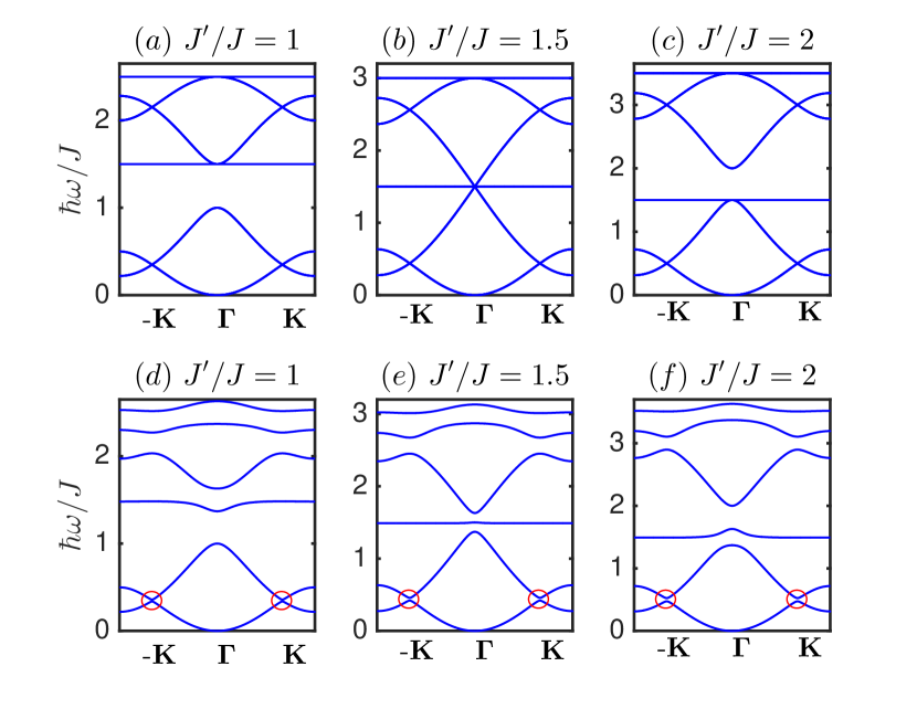
Figure 3: Color online. Magnon bands in the fully polarized ferromagnet at the saturation field $h=h_{s}$. Top panel: $D=0$. Bottom panel: $D/J=0.15$. The circled points are gapped.

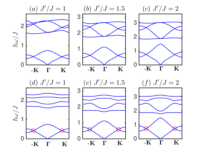
Figure 4: Color online. Magnon bands in the canted antiferromagnet for $h<h_{s}=0.75J$. Top panel: Perpendicular-to-field spin components. Bottom panel: Parallel-to-field spin components. The DM value is $D/J=0.15$. The circled points are gapped.

III.3 Topological magnon bands

We note that the first topological magnon bands have been measured in the kagomé ferromagnet Cu(1-3, bdc) alex6a , thus paving the way to search for topological magnon bands in other systems. In the following we study the topological magnon bands in the star lattice ferromagnet. We consider spin-$1/2$ and take $J$ as the unit of energy while varying $J^{\prime}/J$. We also take the DM value of the kagomé ferromagnet Cu(1-3, bdc) $D/J=0.15$ alex6 ; alex6a . In Fig. 3 we have shown the magnon bands at $D=0$ and $D/J=0.15$ with varying $J^{\prime}/J$. In the former (top panel) the lower bands for $J^{\prime}/J<1.5$ in Fig. 3(a) looks like Dirac magnon on the honeycomb lattice mag . On the other hand, for $J^{\prime}/J>1.5$ the bands in Fig. 3(c) resemble two copies of magnon bands on the kagomé lattice ferromagnet with a flat band and two dispersive Dirac magnon bands on each copy. The gap closes at $J^{\prime}/J=1.5$ as shown in Fig. 3(b). For nonzero DM interaction (lower panel) the the magnon bands are separated by a finite energy gap proportional to the DM interaction in all the parameter regimes. Notice that the collinear ferromagnet at $h=h_{s}$ has a quadratic dispersion (Goldstone mode) at the ${\bf\Gamma}$ point due spontaneous breaking of U(1) symmetry about the $z$-axis. In contrast, for $h<h_{s}$ the spins are canted due to antiferromagnetic interaction between the triangles. This leads to two spin components — perpendicular-to-field spin components and parallel-to-field spin components. In Fig. 4 we have shown the magnon bands in the canted antiferromagnetic phase. Indeed, we recover a linear Goldstone mode at the ${\bf\Gamma}$ point which signifies an antiferromagnetic spin order. In this case the model is no longer an analog of topological fermion insulator on the star lattice zheng2 ; zheng5 ; zheng5a . Furthermore, the perpendicular-to-field spin components (top panel of Fig. 4) show gapless magnon bands even in the presence of DM interaction. A similar gapless magnon bands was reported in the kagomé ferromagnet Cu(1-3, bdc) alex6a when the spins are polarized along the kagomé plane by an in-plane magnetic field. In contrast, the parallel-to-field spin components (bottom panel of Fig. 4) show a finite gap separating the magnon bands due to the presence of DM interaction along the spin polarization.

III.4 Chiral edge modes

The topological aspects of gap Dirac points can be studied by the defining the Berry curvature and the Chern number. In the present model we started from an antiferromagnetic coupled ferromagnets and then recovered a collinear ferromagnetic model. Therefore the Hamiltonian has an off-diagonal terms and the diagonalization requires the generalized Bogoliubov transformation and the eigenfunctions define the Berry curvatures and Chern numbers (see Appendix B). The Chern number vanishes for all bands at zero DM interaction (top panel of Fig. 3). We also find that the Chern number vanishes for the magnon bands of perpendicular-to-field spin components (top panel of Fig. 4). This signifies a trivial magnon insulator. However, we find nonzero Chern numbers for the other magnon bands (bottom panel of Figs. 3 and 4) which defines a topological magnon insulator. A nonzero Chern number is associated with topological chiral gapless magnon edge modes which appear at the DM-induced gaps as shown in Figs. 5 and 6. The edge modes are solved for a strip geometry on the star-lattice with open boundary conditions along the $y$ direction and infinite along the $x$ direction.

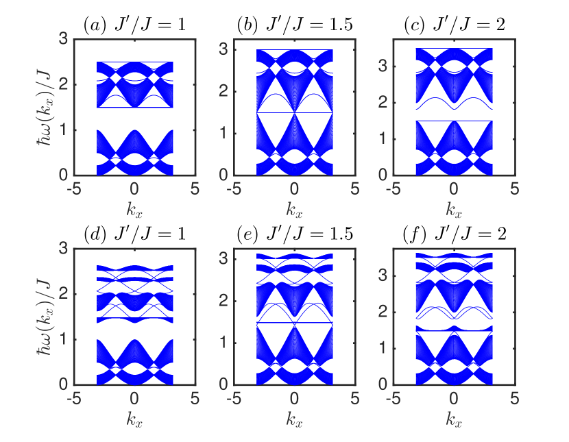
Figure 5: Color online. The corresponding chiral magnon edge modes for Fig. 3.

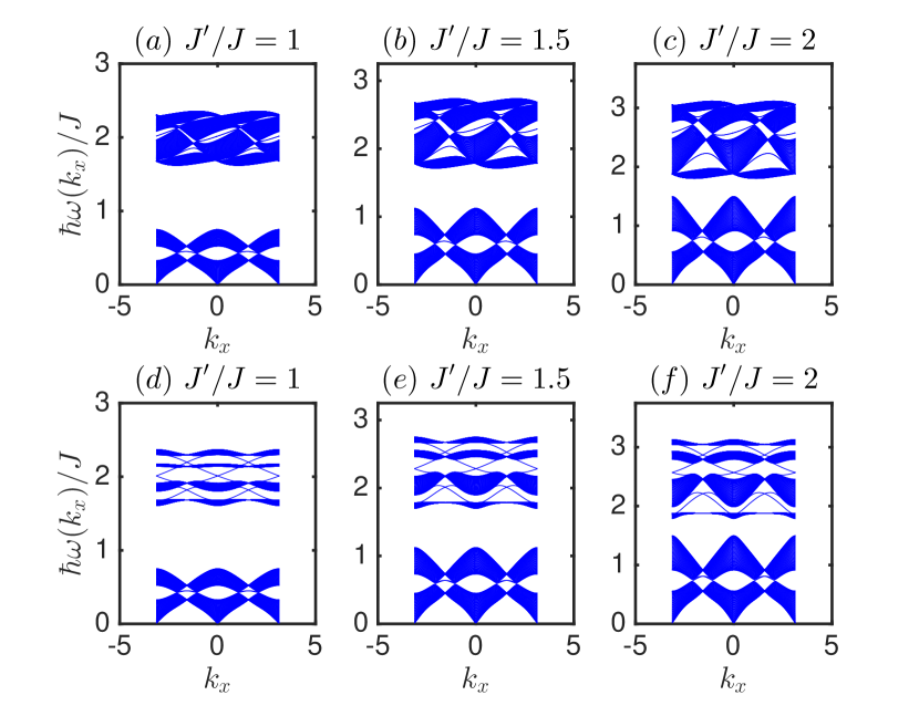
Figure 6: Color online. The corresponding chiral magnon edge modes for Fig. 4.

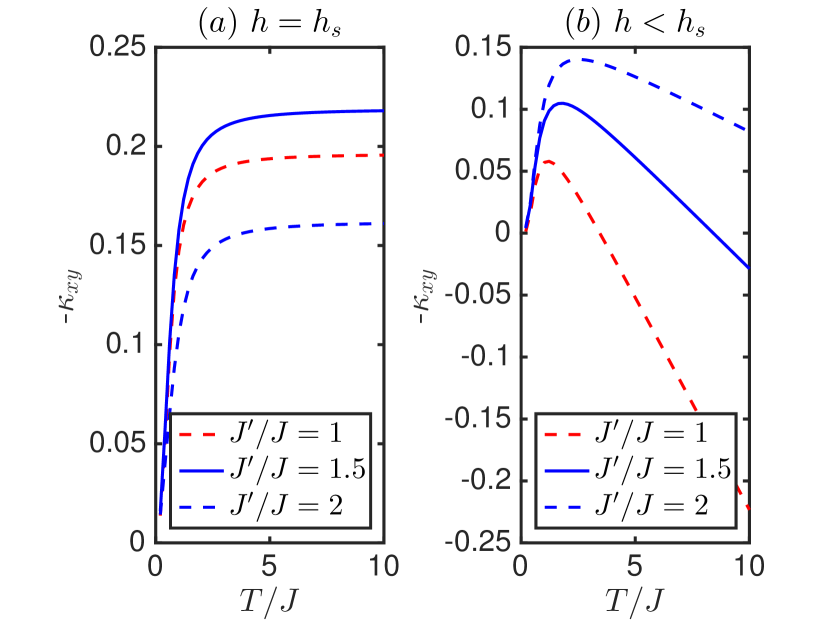
Figure 7: Color online. Low temperature dependence of the thermal Hall conductivity for several values of $J^{\prime}/J$ and $D/J=0.15$.

III.5 Thermal magnon Hall effect

Inelastic neutron scattering experiment has measured the thermal Hall conductivity in the kagomé and pyrochlore ferromagnets alex1 ; alex1a ; alex6 . Theoretically, the thermal Hall effect in insulating ferromagnets is understood as a consequence of the topological magnon bands induced by the DM interaction alex0 . A temperature gradient $-\bm{\nabla}T$ induces a transverse heat current $\mathbb{J}^{Q}$ and the DM-induced Berry curvature acts as an effective magnetic field that deflects the propagation of magnon in the system giving rise to a thermal Hall effect similar to Hall effect in electronic systems. From linear response theory, one obtains $\mathcal{J}_{\alpha}^{Q}=-\sum_{\beta}\kappa_{\alpha\beta}\nabla_{\beta}T$, where $\kappa_{\alpha\beta}$ is the thermal conductivity and the transverse component $\kappa_{xy}$ is associated with thermal Hall conductivity given explicitly as alex2 ; shin1

$$\kappa_{xy}=-\frac{k_{B}^{2}T}{\hbar V}\sum_{\mathbb{k}}\sum_{\alpha=1}^{N}\left(c_{2}[g\left(\omega_{\mathbb{k}\alpha}\right)]-\frac{\pi^{2}}{3}\right)\Omega_{xy;\alpha}(\mathbb{k}),$$ (10)

where $V$ is the volume of the system, $k_{B}$ is the Boltzmann constant, $T$ is the temperature, $g(\omega_{\alpha\mathbb{k}})=[e^{{\omega_{\alpha\mathbb{k}}}/k_{B}T}-1]^{-1}$ is the Bose function, and $c_{2}(x)$ is defined as

$$c_{2}(x)=(1+x)\left(\ln\frac{1+x}{x}\right)^{2}-(\ln x)^{2}-2\text{Li}_{2}(-x),$$ (11)

with $\text{Li}_{2}(x)$ being the dilogarithm. The Berry curvature $\Omega_{xy;\alpha}(\mathbb{k})$ is defined in Appendix B. The thermal Hall conductivity is finite only in the fully polarized collinear ferromagnets at $h=h_{s}$ and the parallel-to-field spin components in the canted antiferromagnet for $h<h_{s}$. As shown in Fig. 7 the thermal Hall conductivity shows a sharp peak and a sign change in the canted phase and vanishes at zero temperature as there are no thermal excitations. This is consistent with the trend observed in previous experiments on the kagomé and pyrochlore ferromagnets alex1 ; alex1a ; alex6 .

IV Conclusion

The star lattice has attracted considerable attention in recent years as an exact solution of Kitaev model zheng1 . Chiral spin liquids, topological fermion insulators and quantum anomalous Hall effect have been proposed zheng ; zheng1 ; zheng3 ; zheng4 ; zheng6 ; zheng2 ; zheng5 ; zheng5a . However, there is no experimental realizations at the moment. In this work, we have contributed to the list of interesting proposals on the star lattice. We have shown that insulating quantum ferromagnets on the star lattice are candidates for topological magnon insulators and thermal magnon Hall transports. We showed that the intrinsic DM interaction which is allowed on the star lattice gives rise to magnetic excitations that exhibit nontrivial magnon bands with non-vanishing Berry curvatures and Chern numbers. We believe that the synthesis of magnetic materials with a star structure is feasible. In fact, experiment has previously realized polymeric iron (III) acetate as a star lattice antiferromagnet with both spin frustration and magnetic long-range order zheng . A strong applied magnetic field is sufficient to induce a ferromagnetic ordered phase in this material and the topological magnon bands can be realized. Unfortunately, inelastic neutron scattering is a bulk sensitive method and the chiral magnon edge modes have not been measured in any topological magnon insulator alex6a . It is possible that edge sensitive methods such as light luuk or electronic kha scattering method can see the chiral magnon edge modes in topological magnon insulators.

Appendix A Free magnon theory

The corresponding free magnon model is achieved by mapping the spin operators to boson operators HP : $S_{i,\tau}^{\prime x}=\sqrt{S/2}(b_{i,\tau}^{\dagger}+b_{i,\tau})$, $S_{i,\tau}^{\prime y}=i\sqrt{S/2}(b_{i,\tau}^{\dagger}-b_{i,\tau})$, and $S_{i,\tau}^{\prime z}=S-b_{i,\tau}^{\dagger}b_{i,\tau}$. The resulting free magnon model is given by

$$\mathcal{H} =v_{0}\sum_{j,\tau}n_{j\tau}-v_{t}\sum_{\langle ij\rangle,\tau}(e^{-i\sigma\phi_{ij}}b^{\dagger}_{i\tau}b_{j\tau}+h.c.)$$

$$-v^{\prime}\sum_{\langle ij\rangle\tau\tau^{\prime}}[(b_{i\tau}^{\dagger}b_{j\tau^{\prime}}+h.c.)\cos^{2}\theta-(b_{i\tau}^{\dagger}b_{j\tau^{\prime}}^{\dagger}+h.c.)\sin^{2}\theta],$$ (12)

where $n_{j\tau}=b_{j\tau}^{\dagger}b_{j\tau}$, $v_{0}=2v_{s}-v_{s}^{\prime}\cos 2\theta+h\cos\theta=2v_{s}+v_{s}^{\prime}$, $v_{s}(v_{s}^{\prime})=JS(J^{\prime}S)$,  $v_{t}=\sqrt{v_{s}^{2}+v_{D_{z(x),\theta}}^{2}}=JS/\cos(\phi_{ij}),~{}v_{D_{\parallel(\perp),\theta}}=D_{\parallel(\perp),\theta}S$; $\phi_{ij}=\pm\phi=\arctan(D_{\parallel(\perp),\theta}/J)$ is a magnetic flux generated by the DM interaction within the triangular plaquettes, similar to Haldane model fdm . For ${\bf D}\parallel{\bf H}$, $\sigma=1$ and for ${\bf D}\perp{\bf H}$, $\sigma=\pm 1$ for sublattice $\mathcal{A}$ and $\mathcal{B}$ respectively. The configurations of $\phi_{ij}$ for both cases are depicted in Fig. 2. The total flux in the dodecagon consisting of twelve sites is $-2\phi$ and $0$ respectively. Indeed, $\phi_{ij}$ vanishes along the $J^{\prime}$ link as it contains no triangular plaquettes.

The momentum space Hamiltonian can be written as $\mathcal{H}=\frac{1}{2}\sum_{\mathbb{k}}\psi^{\dagger}_{\mathbb{k}}\cdot\bm{\mathcal{H}}(\mathbb{k})\cdot\psi_{\mathbb{k}},$ with $\psi^{\dagger}_{\mathbb{k}}=(b_{\mu,\mathbb{k}}^{\dagger},\thinspace b_{\mu^{\prime},\mathbb{k}}^{\dagger},b_{\mu,-\mathbb{k}},\thinspace b_{\mu^{\prime},-\mathbb{k}})$, where $\mu=1,2,3$ and $\mu^{\prime}=4,5,6$. The Bogoliubov Hamiltonian $\mathcal{H}(\mathbb{k})$ is a $2N\times 2N$ matrix given by

$$\bm{\mathcal{H}}(\mathbb{k})=\begin{pmatrix}\mathbb{A}(\mathbb{k},\phi)&\mathbb{B}(\mathbb{k})\\ \mathbb{B}^{*}(-\mathbb{k})&\mathbb{A}^{*}(-\mathbb{k},\phi)\end{pmatrix},$$ (13)

where

$$\mathbb{A}(\mathbb{k})=\begin{pmatrix}\mathbb{a}(\sigma\phi)&\mathbb{b}_{1}(\mathbb{k})\\ \mathbb{b}_{1}(-\mathbb{k})&\mathbb{a}(\sigma\phi)\end{pmatrix},~{}\mathbb{B}(\mathbb{k})=\begin{pmatrix}{\bf 0}&\mathbb{b}_{2}(\mathbb{k})\\ \mathbb{b}_{2}(-\mathbb{k})&{\bf 0}\end{pmatrix},$$ (14)

$$\mathbb{a}(\sigma\phi)=\begin{pmatrix}v_{0}&-v_{t}e^{-i\sigma\phi}&-v_{t}e^{i\sigma\phi}\\ -v_{t}e^{i\sigma\phi}&v_{0}&-v_{t}e^{-i\sigma\phi}\\ -v_{t}e^{-i\sigma\phi}&-v_{t}e^{i\sigma\phi}&v_{0}\end{pmatrix},$$ (15)

$$\mathbb{b}_{1}(\mathbb{k})=-v_{s}^{\prime}\cos^{2}\theta\begin{pmatrix}e^{ik_{2}}&0&0\\ 0&e^{ik_{1}}&0\\ 0&0&1\end{pmatrix},$$ (16)

$$\mathbb{b}_{2}(\mathbb{k})=v_{s}^{\prime}\sin^{2}\theta\begin{pmatrix}e^{ik_{2}}&0&0\\ 0&e^{ik_{1}}&0\\ 0&0&1\\ \end{pmatrix},$$ (17)

where $k_{1}=\mathbb{k}\cdot\mathbb{a}_{1}$ and $k_{2}=\mathbb{k}\cdot\mathbb{a}_{2}$. The lattice basis vectors are chosen as $\mathbb{a}_{1}=2\hat{\mathbb{x}}$ and $\mathbb{a}_{2}=\hat{\mathbb{x}}+\sqrt{3}\hat{\mathbb{y}}$. At the saturation field $h=h_{s}(\theta=0)$ the spins are fully aligned along the $z$-axis and $\mathbb{b}_{2}(\mathbb{k})=0$. We therefore recover collinear ferromagnet along the $z$-direction. The Hamiltonian is diagonalized below.

Appendix B Berry curvature and Chern number

To diagonalize the Hamiltonian we make a linear transformation $\psi_{\mathbb{k}}=\mathcal{P}_{\mathbb{k}}Q_{\mathbb{k}}$, where $\mathcal{P}_{\mathbb{k}}$ is a $2N\times 2N$ paraunitary matrix and $Q^{\dagger}_{\mathbb{k}}=(\mathcal{Q}_{\mathbb{k}}^{\dagger},\thinspace\mathcal{Q}_{-\mathbb{k}})$ with $\mathcal{Q}_{\mathbb{k}}^{\dagger}=(\gamma_{\mathbb{k}\mu}^{\dagger},\thinspace\gamma_{\mathbb{k}\mu^{\prime}}^{\dagger})$ being the quasiparticle operators. The matrix $\mathcal{P}_{\mathbb{k}}$ satisfies the relations,

$$\mathcal{P}_{\mathbb{k}}^{\dagger}\bm{\mathcal{H}}(\mathbb{k})\mathcal{P}_{\mathbb{k}}=\mathcal{E}_{\mathbb{k}},$$ (18)

$$\mathcal{P}_{\mathbb{k}}^{\dagger}\bm{\tau}_{3}\mathcal{P}_{\mathbb{k}}=\bm{\tau}_{3},$$ (19)

where $\mathcal{E}_{\mathbb{k}}=\text{diag}(\omega_{\mathbb{k}\alpha},~{}\omega_{-\mathbb{k}\alpha})$, $\bm{\tau}_{3}=\text{diag}(\mathbf{I}_{N\times N},-\mathbf{I}_{N\times N})$, and $\omega_{\mathbb{k}\alpha}$ are the energy eigenvalues and $\alpha$ labels the bands. From Eq. 19 we get $\mathcal{P}_{\mathbb{k}}^{\dagger}=\bm{\tau}_{3}\mathcal{P}_{\mathbb{k}}^{-1}\bm{\tau}_{3}$, and Eq. 18 is equivalent to saying that we need to diagonalize the Hamiltonian $\bm{\mathcal{H}}^{\prime}(\mathbb{k})=\bm{\tau}_{3}\bm{\mathcal{H}}(\mathbb{k}),$ whose eigenvalues are given by $\bm{\tau}_{3}\mathcal{E}_{\mathbb{k}}$ and the columns of $\mathcal{P}_{\mathbb{k}}$ are the corresponding eigenvectors. The eigenvalues of this Hamiltonian cannot be obtained analytically except at zero field. The paraunitary operator $\mathcal{P}_{\mathbb{k}}$ defines a Berry curvature given by

$$\Omega_{ij;\alpha}(\mathbb{k})=-2\text{Im}[\bm{\tau}_{3}\mathcal{(}\partial_{k_{i}}\mathcal{P}_{\mathbb{k}\alpha}^{\dagger})\bm{\tau}_{3}(\partial_{k_{j}}\mathcal{P}_{\mathbb{k}\alpha})]_{\alpha\alpha},$$ (20)

with $i,j=\{x,y\}$ and $\mathcal{P}_{\mathbb{k}\alpha}$ are the columns of $\mathcal{P}_{\mathbb{k}}$. In this form, the Berry curvature simply extracts the diagonal components which are the most important. From Eq. 18 the Berry curvature can be written alternatively as

$$\Omega_{ij;\alpha}(\mathbb{k})=-\sum_{\alpha^{\prime}\neq\alpha}\frac{2\text{Im}[\braket{\mathcal{P}_{\mathbb{k}\alpha}}{v_{i}}{\mathcal{P}_{\mathbb{k}\alpha^{\prime}}}\braket{\mathcal{P}_{\mathbb{k}\alpha^{\prime}}}{v_{j}}{\mathcal{P}_{\mathbb{k}\alpha}}]}{\left(\omega_{\mathbb{k}\alpha}-\omega_{\mathbb{k}\alpha^{\prime}}\right)^{2}},$$ (21)

where $\mathbb{v}=\partial\bm{\mathcal{H}}^{\prime}(\mathbb{k})/\partial\mathbb{k}$ defines the velocity operators. The Berry curvature is related to DM interaction $\Omega(\mathbb{k})\propto\phi$ and the Chern number is defined as,

$$\mathcal{C}_{\alpha}=\frac{1}{2\pi}\int_{{BZ}}dk_{x}dk_{y}~{}\Omega_{xy;\alpha}(\mathbb{k}).$$ (22)

References

- (1) V. V. Kruglyak, S. O. Demokritov, and D. Grundler, J. Phys. D: Appl. Phys. 43, 264001 (2010).
- (2) Benjamin Lenk, Henning Ulrichs, Fabian Garbs, Markus Münzenberg, Physics Reports 507, 107 (2011).
- (3) A. V. Chumak et al., Nature Physics 11, 453 (2015).
- (4) I. Dzyaloshinsky J. Phys. Chem. Solids 4, 241 1958; T. Moriya Phys. Rev. 120, 91 (1960).
- (5) T. Moriya Phys. Rev. 120, 91 (1960).
- (6) H. Katsura, N. Nagaosa, and P. A. Lee Phys. Rev. Lett. 104, 066403 (2010).
- (7) Y. Onose et al., Science 329, 297 (2010).
- (8) T. Ideue et al., Phys. Rev. Lett. 85, 134411 (2012).
- (9) Max Hirschberger et al., Phys. Rev. Lett. 115, 106603 (2015).
- (10) R. Chisnell et al., Phys. Rev. Lett. 115, 147201 (2015).
- (11) R. Matsumoto and S. Murakami Phys. Rev. Lett. 106, 197202 (2011); Phys. Rev. B 84, 184406 (2011).
- (12) A. A. Kovalev and V. Zyuzin, Phys. Rev. B 93, 161106(R) (2016).
- (13) M. Hirschberger et al., Science 348, 106 (2015).
- (14) R. Shindou et.al., Phys. Rev. B 87, 174427 (2013); Phys. Rev. B 87, 174402 (2013).
- (15) R. Matsumoto, R. Shindou, and S. Murakami, Phys. Rev. B 89, 054420 (2014).
- (16) L. Zhang et al., Phys. Rev. B 87, 144101 (2013).
- (17) H. Lee, J. H. Han, and P. A. Lee Phys. Rev. B. 91, 125413 (2015) .
- (18) A. Mook, J. Henk, and I. Mertig Phys. Rev. B 90, 024412 (2014); A. Mook, J. Henk, and I. Mertig, Phys. Rev. B 89, 134409 (2014).
- (19) J. H. Han, H. Lee, J. Phys. Soc. Jpn. 86, 011007 (2017).
- (20) S. A. Owerre, J. Phys.: Condens. Matter 28, 386001 (2016).
- (21) S. A. Owerre, J. Appl. Phys. 120, 043903 (2016).
- (22) Se Kwon Kim et al., Phys. Rev. Lett. 117, 227201 (2016).
- (23) A. Mook, J. Henk, and I. Mertig, Phys. Rev. Lett. 117, 157204 (2016).
- (24) Ying Su, X. S. Wang, X. R. Wang, arXiv:1609.01500 (2016).
- (25) H. Yao and S. A. Kivelson, Phys. Rev. Lett. 99, 247203 (2007).
- (26) Heng-Fu Lin et al., Phys. Rev. A 90, 053627 (2014).
- (27) Y. -Z. Zheng et al., Angew. Chem., Int. Ed. 46, 6076 (2007).
- (28) J. O. Fjaerestad, arXiv:0811.3789.
- (29) B.-J. Yang, A. Paramekanti, and Y. B. Kim, Phys. Rev. B 81, 134418 (2010).
- (30) A. Rüegg, J. Wen, and G. A. Fiete, Phys. Rev. B 81, 205115 (2010).
- (31) Wen-Chao Chen et al., Phys. Rev. B 86, 085311 (2012).
- (32) Mengsu Chen and Shaolong Wan, J. Phys.: Condens. Matter 24, 325502 (2012).
- (33) T. Holstein and H. Primakoff, Phys. Rev. 58, 1098 (1940).
- (34) F. D. M. Haldane Phys. Rev. Lett. 61, 2015 (1988).
- (35) J. Fransson, A. M. Black-Schaffer, and A. V. Balatsky, Phys. Rev. B 94, 075401 (2016).
- (36) Luuk J. P. Ament, Michel van Veenendaal, Thomas P. Devereaux, John P. Hill, and Jeroen van den Brink, Rev. Mod. Phys. 83, 705 (2011).
- (37) Khalil Zakeri, Physics Reports 545, 47 (2014).