A Convex Relaxation Approach to Higher-Order Statistical Approaches to Signal Recovery

Abstract

In this work, we investigate an efficient numerical approach for solving higher order statistical methods for blind and semi-blind signal recovery from non-ideal channels. We develop numerical algorithms based on convex optimization relaxation for minimization of higher order statistical cost functions. The new formulation through convex relaxation overcomes the local convergence problem of existing gradient descent based algorithms and applies to several well-known cost functions for effective blind signal recovery including blind equalization and blind source separation in both single-input-single-output (SISO) and multi-input-multi-output (MIMO) systems. We also propose a fourth order pilot based cost function that benefits from this approach. The simulation results demonstrate that our approach is suitable for short-length packet data transmission using only a few pilot symbols.

Keywords: Blind signal recovery, semi/blind channel equalization, convex optimization, semidefinite programming, rank 1 approximation.

I Introduction

Blind signal recovery is a well-known problem in signal processing and communications. With a special goal of recovering unknown input signals to unknown linear systems based on the system output signals, this problem typically manifests itself either as blind equalization or blind source separation. In SISO systems or single-input-multiple-output (SIMO) systems, the goal of channel equalization is to undo the inter-symbol interference (ISI). In MIMO systems or in source separation, the objective is to mitigate both the ISI and the inter-channel interference (ICI) in order to successfully separate different sources. The advantage lies in the fact that blind algorithms do not require allocation of extra bandwidth to training signals whereas semiblind algorithms can substantially reduce the length of training signals. System implementations based on blind algorithms have appeared in downstream cable modem [1], HDTV [2, 3, 4].

The specially designed cost functions for blind signal recovery typically pose a challenge to the issue of global convergence and convergence speed. In literature, global convergent algorithms for blind equalization and source separation do exist for linear programming equalization [5] and space-time signal detection [6]. However, without limiting system input signals to the special QAM class, most of the blind algorithms are based on non-quadratic and non-convex costs that utilize high-order statistics of the received signals. Well-known algorithms of this type include the constant modulus algorithm (CMA) [7, 8], the Shalvi-Weinstein algorithm (SWA) [9], and the minimum entropy deconvolution (MED) algorithm [10, 11]. In fact, without modifications, these stochastic gradient descent (SGD) algorithms typically admit multiple local minima [12, 13] and require large numbers of data and iterations to converge.

To improve convergence speed of blind channel equalization techniques, batch algorithms can effectively utilize the statistical information of the channel output signals. They can significantly shorten the convergence time [14, 15, 16, 17, 18, 19]. Unfortunately, local convergence remains a major obstacle, that requires good initialization strategies. Another approach to mitigate the local convergence problem is through relaxation by “lifting” the receiver parameters to a new parameterization that covers a larger parameter space over which the cost function is convex [20, 21]. Once the convex problem is uniquely solved, the solution is mapped back to the original restrictive parameter space. For example, the authors of [20] relaxed the outer-product matrix of the equalizer parameter space from a rank-1 matrix to an unrestricted square matrix over which the CMA cost becomes quadratic and can be solved globally via least squares (LS). From the relaxed solution, a series of linear operations map the solution back into the right equalizer coefficient space. In [21], the authors proposed a similar relaxation with a much more elegant algorithm that modifies the CMA cost function into a special sum. The modified CMA cost is first solved over a more restrictive semi-definite positive matrix space. The resulting convex optimization problem is then solved efficiently via semidefinite programing (SDP). Iterative mappings must also follow the SDP solution in order to determine the equalizer parameters [21].

In this work, we study means to improve the convergence of general blind and semiblind equalization algorithms by generalizing the cost modification principle presented in [21]. We can therefore develop a more general batch implementation of well-known blind equalization and source separation algorithms that minimize cost functions involving the fourth order statistics of system output signals. More specifically, the new implementation leverages a convex optimization relaxation that can be applied to CMA, SWA, and MED algorithms. We show that our convex formulation requires less resource and improves the efficiency of the convex formulation in [21]. We further generalize the formulation to accommodate the semi-blind algorithms when a small number of training symbols are available to assist the receiver signal recovery and separation. Our proposed method overcomes the local convergence problem which is a drawback of traditional gradient descent implementations.

The rest of the paper is organized as follows. In Section II, we introduce MIMO system model. Section III discusses batch MIMO blind source recovery using CMA cost as an example of real-valued fourth order functions. Section IV presents a convex formulation of the fourth order function and algorithm to find its global minima. In Section V, we extend formulation to other blind algorithms based on fourth order cost. A semiblind algorithm using fourth order function is proposed in Section VI. In Section VII, we present our simulation results and Section VIII contains some concluding remarks. In the Appendices, we include the formulation of converting cross-correlation cost and the training based cost into real-valued fourth order functions.

II Problem Statement and System Model

We consider a baseband MIMO system model with $N_{\text{T}}$ transmit antennas and $N_{\text{R}}$ receive antennas. This MIMO model covers SIMO and SISO channels. Let $s_{n}\left(k\right)$, $n=1,\ldots,N_{\text{T}}$ denote random independent data symbols for transmit antenna $n$ at time $k$. $\{s_{n}\}$ typically belong to finite set ${\cal A}$. Consistent with practical QAM systems, we assume that $s_{n}\left(k\right)$ are mutually independent and identically distributed (i.i.d.) with variance $\sigma_{s}^{2}$ and fourth order kurtosis $\gamma_{s}<0$.

The data streams are transmitted over multipath MIMO channels denoted by impulse responses $h_{j,n}\left(m\right)$, $n=1,\ldots,N_{\text{T}}$, $j=1,\ldots,N_{\text{R}}$, $m=0,\ldots,L_{h}$, with delay spread of $L_{h}+1$ samples. Assuming the MIMO channel is corrupted by i.i.d. additive white Gaussian noise (AWGN) $v_{j}\left(k\right)$ with zero-mean and variance $\sigma_{v}^{2}$, the output of $j$-th receiver can be expressed as

$$x_{j}\left(k\right) = \sum_{n=1}^{N_{\text{T}}}\sum_{m=0}^{L_{h}}h_{j,n}\left(m\right)s_{n}(k-m)+v_{j}\left(k\right).$$ (1)

The goal of the MIMO receiver is to recover data stream $s_{n}\left(k\right)$, $n=1,\ldots,N_{\text{T}}$ from the channel output $\{x_{j}\left(k\right)\}$. Following most of the works in this area, we shall focus only on linear FIR equalizers. Given $N_{\text{R}}$ sub-channel outputs, we apply a $N_{\text{T}}\times N_{\text{R}}$ MIMO equalizer with parameter vector

$$\mathbf{w}_{i,j}=\left[w_{i,j}\left(0\right)\>w_{i,j}\left(1\right)\ldots w_{i,j}\left(L_{w}\right)\right]^{T}$$

where $L_{w}$ is considered as the order of individual equalizer and $i=1,\ldots,N_{\text{T}}$, $j=1,\ldots,N_{\text{R}}$. If the channel is flat fading (or non-frequency-selective), then we have a degenerated problem of blind source separation for which $L_{h}=0$. The FIR blind MIMO equalizer then degenerates into a linear source separation matrix $\mathbf{W}=[w_{i,j}(0)]$.

The linear receiver output has $N_{\text{T}}$ parallel output streams denoted by

$$y_{i}\left(k\right) =\sum_{j=1}^{N_{\text{R}}}w_{i,j}^{*}\left(k\right)\circledast x_{j}(k)$$

$$=\sum_{j=1}^{N_{\text{R}}}\sum_{\ell=0}^{L_{w}}w_{i,j}^{*}\left(\ell\right)x_{j}(k-\ell)$$ (2)

where $\circledast$ denote the convolution. Our objective is to optimize the linear receiver parameters $\{w_{i,j}(n)\}$ such that the source data symbols are recovered by $y_{i}\left(k\right)$ without interference as follows

$$y_{i}\left(k\right)=e^{j\phi_{i}}s_{q_{i}}(k-k_{i})+\mbox{residual noise}.$$

Note that $\phi_{i}$ is a phase ambiguity that is inherent to the blind signal recovery which cannot be resolved without additional information; and $k_{i}$ is the output delay of the $q_{i}-$th signal recovery that does not affect the receiver performance. Upon optimum convergence, a simple memoryless decision device $\mbox{dec}(\cdot)$ can be applied, and at high signal to noise ratio (SNR), we have

$$\hat{s}_{i}(k-k_{i})=\mbox{dec}\left[y_{i}(k)\right]=s_{q_{i}}(k-k_{i}).$$

For convenience of notation, we further define

$$\mathbf{w}_{i} =\left[\mathbf{w}_{i,1}^{T}\>\mathbf{w}_{i,2}^{T}\ldots\mathbf{w}_{i,N_{\text{R}}}^{T}\right]^{T},$$

$$\mathbf{x}_{j}\left(k\right) =\left[x_{j}\left(k\right)\>x_{j}\left(k-1\right)\ldots x_{j}\left(k-L_{w}\right)\right]^{T},$$

$$\mathbf{x}\left(k\right) =\left[\mathbf{x}_{1}^{T}\left(k\right)\>\mathbf{x}_{2}^{T}\left(k\right)\ldots\mathbf{x}_{N_{\text{R}}}^{T}\left(k\right)\right]^{T}.$$

With these notations, we can write

$$y_{i}\left(k\right) =\sum_{j=1}^{N_{\text{R}}}\mathbf{w}_{i,j}^{H}\mathbf{x}_{j}(k)=\mathbf{w}_{i}^{H}\mathbf{x}(k)$$

$$=\sum_{n=1}^{N_{\text{T}}}\underbrace{\left(\sum_{j=1}^{N_{\text{R}}}w_{i,j}^{*}\left(k\right)\circledast h_{j,n}\left(k\right)\right)}_{\mbox{combined response }c_{i,n}^{*}\left(k\right)}\circledast s_{n}(k)$$

$$+\underbrace{\sum_{j=1}^{N_{\text{R}}}w_{i,j}^{*}\left(k\right)\circledast v_{j}(k)}_{\mbox{Gaussian noise $\eta_{i}\left(k\right)$}}$$ (3)

$$=\sum_{n=1}^{N_{\text{T}}}c_{i,n}^{*}\left(k\right)\circledast s_{n}(k)+\eta_{i}\left(k\right).$$ (4)

In MIMO blind equalization, we would like to find equalizer parameter vectors $\mathbf{w}_{i}$ such that the combined (channel-equalizer) response is free of inter-symbol and inter-channel interferences

$$c_{i,n}\left(k\right)=\begin{cases}e^{j\phi_{i}}&\text{for }k=k_{i},\>n=q_{i}\\ 0&\text{otherwise}.\end{cases}$$ (5)

III Constant Modulus Algorithm for MIMO Equalization

In this section, we provide a real-valued representation of the conventional batch CMA cost. This representation is one of the keys to reduce parameter space compared to the work of [21] in which the formulation is based on complex values. This representation is also applied to other blind channel equalization and blind source separation costs and will be shown in the latter sections.

III-A CMA for single source recovery

For the sake of clarity, we discuss the CMA cost as an example of selecting blind cost. To recover a particular source, the CMA cost function for the $i$-th equalizer output sequence is defined as

$$J_{\text{b},i}=J_{\text{cma},i}=E\left[\left(|y_{i}(k)|^{2}-R_{2}\right)^{2}\right]$$ (6)

where $R_{2}=\frac{E\left[\left|s_{i}\left(k\right)\right|^{4}\right]}{E\left[\left|s_{i}\left(k\right)\right|^{2}\right]}$. The CMA cost can be represented as a function of the equalizer coefficients and the channel output statistics [22]. Since the formulation here deals with single source, the source index $i$ is omitted.

Let $\text{Re}\left\{\boldsymbol{x}\right\}$ and $\text{Im}\left\{\boldsymbol{x}\right\}$ denote the real and imaginary parts of $\boldsymbol{x}$. Now define $\mathbf{u}=\left[\begin{array}[]{c}\text{Re}\left\{\mathbf{w}\right\}\\ \text{Im}\left\{\mathbf{w}\right\}\end{array}\right]$, $\mathbf{x}_{\text{r}}(k)=\left[\begin{array}[]{c}\text{Re}\left\{\mathbf{x}(k)\right\}\\ \text{Im}\left\{\mathbf{x}(k)\right\}\end{array}\right]$ and $\mathbf{x}_{\text{i}}(k)=\left[\begin{array}[]{c}\text{Im}\left\{\mathbf{x}(k)\right\}\\ -\text{Re}\left\{\mathbf{x}(k)\right\}\end{array}\right]$. We have the following relationship

$$\text{Re}\left\{y\left(k\right)\right\} = \mathbf{u}^{T}\mathbf{x}_{\text{r}}(k),$$ (7)

$$\text{Im}\left\{y\left(k\right)\right\} = \mathbf{u}^{T}\mathbf{x}_{\text{i}}(k).$$ (8)

As a result, we have

$$\begin{split}\left|y\left(k\right)\right|^{2}&=\text{Re}^{2}\left\{y\left(k\right)\right\}+\text{Im}^{2}\left\{y\left(k\right)\right\}\\ &=\mathbf{u}^{T}\mathbf{x}_{\text{r}}(k)\mathbf{x}_{\text{r}}(k)^{T}\mathbf{u}+\mathbf{u}^{T}\mathbf{x}_{\text{i}}(k)\mathbf{x}_{\text{i}}(k)^{T}\mathbf{u}\\ &=\mathbf{u}^{T}\underbrace{\left[\mathbf{x}_{\text{r}}(k)\mathbf{x}_{\text{r}}^{T}(k)+\mathbf{x}_{\text{i}}(k)\mathbf{x}_{\text{i}}^{T}(k)\right]}_{\bar{\mathbf{X}}_{k}}\mathbf{u}.\end{split}$$ (9)

By denoting the rank-1 matrix $\bar{\mathbf{X}}_{k}=\mathbf{x}_{\text{r}}(k)\mathbf{x}_{\text{r}}^{T}(k)+\mathbf{x}_{\text{i}}(k)\mathbf{x}_{\text{i}}^{T}(k)$ and $\mathbf{U}=\mathbf{u}\mathbf{u}^{T}$, we have

$$\left|y\left(k\right)\right|^{2}=\text{Tr}\left(\bar{\mathbf{X}}_{k}\mathbf{U}\right).$$ (10)

Note that both $\bar{\mathbf{X}}_{k}$ and $\mathbf{U}$ are symmetric of dimension $2N\times 2N$ with $N=L_{w}+1$. In other words, $\bar{\mathbf{X}}_{k}$ and $\mathbf{U}$ can be mapped by the svec$\left(\cdot\right)$ operator to lower dimensional subspace $\mathbb{R}^{N\left(2N+1\right)}$ after ignoring redundant entries. Furthermore, we sort the entries in the usual lexicographic order. We define the following operators and vectors:

• For a symmetric $2N\times 2N$ matrix $\mathbf{X}$, we define svec$\left(\cdot\right)$ operator and its reverse operator $\mbox{svec}^{-1}\left(\cdot\right)$ as

  $$\begin{split}\text{svec}\left(\mathbf{X}\right)&=\left[X_{1,1}\>2X_{1,2}\ldots\>2X_{1,2n}\>X_{2,2}\right.\\ &\quad\left.2X_{2,3}\ldots 2X_{2,2N}\ldots X_{2N,2N}\right]^{T}\in\mathbb{R}^{N(2N+1)},\\ \mathbf{X}&=\mbox{svec}^{-1}\left(\text{svec}\left(\mathbf{X}\right)\right).\end{split}$$ (11)

• For a vector $\mathbf{u}\in\mathbb{R}^{2N}$, we define $\mathbf{v}=\mbox{qvec}(\mathbf{u})$ as vector whose entries are all second order (quadratic) terms $\left\{u_{i}u_{j}\right\}$ and sorted in the usual lexicographic order.

  $$\begin{split}\mathbf{v}&=\mbox{qvec}(\mathbf{u})\\ &=[u_{1}u_{1}\>u_{1}u_{2}\ldots u_{1}u_{2n}\>u_{2}u_{2}\>u_{2}u_{3}\>\ldots\\ &\quad\;\;u_{2}u_{2N}\ldots u_{2N}u_{2N}]^{T}.\end{split}$$ (12)

  There is one to one mapping between elements of $\mathbf{v}$ and $\mathbf{U}=\mathbf{u}\mathbf{u}^{T}$ as $\mathbf{v}$ consists of all upper triangle elements of $\mathbf{U}$. Nevertheless, the reverse operator needs further consideration. Given an arbitrary $\mathbf{v}\in\mathbb{R}^{2N^{2}+N+1}$, we can form the corresponding $\mathbf{U}$, which is not necessarily a rank 1 matrix. Therefore, we define the reverse operator with approximation $\mbox{qvec}^{-1}(\mathbf{v})$ as follows: First, using $\mathbf{v}$ to form the corresponding $\mathbf{U}$; Next, find the rank 1 approximation of $\mathbf{U}$ by its maximum eigenvalue $\lambda_{\mathbf{U}}$ and the corresponding eigenvector $\mathbf{u}_{\text{eig}}$. The resulting matrix is ${\lambda_{\mathbf{U}}}\mathbf{u}_{\text{eig}}\mathbf{u}^{T}_{\text{eig}}$.

With the above definitions, the output power can be rewritten as

$$\begin{split}E\left[\left|y\left(k\right)\right|^{2}\right]&=E\left[\mathbf{v}^{T}\text{svec}\left(\bar{\mathbf{X}}_{k}\right)\right]=\mathbf{v}^{T}\text{svec}\left(E\left[\bar{\mathbf{X}}_{k}\right]\right)\\ &=\mathbf{v}^{T}\underset{\mathbf{b}}{\underbrace{E\left[\text{svec}\left(\bar{\mathbf{X}}_{k}\right)\right]}}=\mathbf{v}^{T}\mathbf{b}.\end{split}$$ (13)

Similarly, the fourth order moment of equalizer output is

$$E\left[\left|y\left(k\right)\right|^{4}\right] = \mathbf{v}^{T}\underset{\mathbf{C}}{\underbrace{E\left[\text{svec}\left(\bar{\mathbf{X}}_{k}\right)\text{svec}^{T}\left(\bar{\mathbf{X}}_{k}\right)\right]}}\mathbf{v}$$ (14)

$$= \mathbf{v}^{T}\mathbf{C}\mathbf{v}.$$

Therefore, the CMA cost can be written into a fourth order function of $\mathbf{u}$ or a quadratic function of $\mathbf{v}$ as

$$J_{\text{cma}} = \mathbf{v}^{T}\mathbf{C}\mathbf{v}-2R_{2}\mathbf{b}^{T}\mathbf{v}+R_{2}^{2}.$$ (15)

The equalizer can be found by minimizing the polynomial function $J_{\text{cma}}$.

III-B Multi-source recovery

To recover multiple input source signals of a MIMO channel, we must form several single stream receivers $\{\mathbf{w}_{i}\}$ to generate multiple receiver output streams $\{y_{i}(k)\}$ that will represent distinct source signals $\{s_{q_{i}}(k)\}$. Typically, a blind algorithm is adept at recovering one of the possible source signals. However, because of the inherent properties of blind equalization, the receiver is unable to ascertain which signal may be recovered a priori. As a result, multiple single stream receivers may recover duplicate signals and miss some critical source signals. To avoid duplicate convergence, proper initialization of each $\mathbf{w}_{i}$ may help lead to a diversified convergence as needed. However, there is unfortunately no guarantee that different initial values of $\mathbf{w}_{i}$ will lead to $q_{i}\not=q_{j}$. In order to ensure that different receiver vectors $\mathbf{w}_{i}$ extract distinct signals, common criteria rely on the prior information that the source signals are i.i.d. and mutually independent.

Let $J_{\text{b},i}$ denote a blind cost function, for examples, CMA, SWA, or MED, to recover the source $i$, the cost function for multiple blind source recovery (BSR) is [23, 24]

$$J_{\text{bsr}}=\sum_{i=1}^{N_{\text{T}}}J_{\text{b},i}+\lambda_{\text{cr}}\cdot\sum_{i\neq j}^{N_{\text{T}}}J_{\text{cr},i,j}$$ (16)

where $\lambda_{\text{cr}}$ is a positive scalar and $J_{\text{cr},i,j}$ accounts for the correlation of the receiver outputs $i$ and $j$. The minimization of $J_{\text{cr},i,j}$ ensures that the equalizers converge to different solutions corresponding to different sources. One can recover all sources either simultaneously or sequentially to reduce the parameter size.

In sequential source recovery, we start by extracting the first source by minimizing one single CMA cost. Assume the sources up to $j-1$ are equalized and separated, we can minimize the following cost for separating the source $j$.

$$J_{\text{bsr},j}=J_{\text{b},j}+\lambda_{\text{cr}}\sum_{i=1}^{j-1}J_{\text{cr},i,j}.$$ (17)

In this work, we consider the sequential approach. $J_{\text{cr},i,j}$ can be chosen as the sum of cross-cumulants [24] or as the sum of cross-correlations [23]. Since the use of cross-cumulant is for coarse step separation [24] and may lead to poor convergence, here, we use the cross-correlation

$$J_{\text{cr},i,j}=\sum_{l=-\delta}^{\delta}\left|E\left[y_{i}\left(k\right)y_{j}^{*}\left(k-l\right)\right]\right|^{2}$$ (18)

where $\delta$ is an integer parameter to be chosen during system design. $J_{\text{cr},i,j}$ can also be written as a fourth order function of $\mathbf{u}_{j}$ or a second order function of $\mathbf{v}_{j}=\mbox{qvec}(\mathbf{u}_{j})$. Noticing that $\mathbf{u}_{i}$, for $i<j$, are already known, we can write

$$\sum_{i=1}^{j-1}J_{\text{cr},i,j}=\mathbf{q}_{j}^{T}\mathbf{v}_{j}$$ (19)

where $\mathbf{q}_{j}$ is a vector formed by the previously calculated equalizers and received statistics. The detailed calculation of $\mathbf{q}_{j}$ is given in the Appendix A.

Eventually, the cost in (17) when using CMA and cross-correlation can be written as a fourth order (cost) function of equalizer parameter with zero odd-order coefficients similar to $J_{\text{cma}}$:

$$J_{\text{bsr},j} =f(\mathbf{u}_{j})$$

$$=\mathbf{v}_{j}^{T}\mathbf{C}\mathbf{v}_{j}-2R_{2}\mathbf{b}^{T}\mathbf{v}_{j}+R_{2}^{2}+\lambda_{\text{cr}}\mathbf{q}_{j}^{T}\mathbf{v}_{j}$$

$$=\mathbf{v}_{j}^{T}\mathbf{C}\mathbf{v}_{j}-\left(2R_{2}\mathbf{b}^{T}-\lambda_{\text{cr}}\mathbf{q}_{j}^{T}\right)\mathbf{v}_{j}+R_{2}^{2}.$$ (20)

In the following section, we discuss the method to find global minima of the functions of this type.

IV Semidefinite programming approach to minimize a fourth order polynomial

IV-A General formulation

General formula to find the global minimum of a non-negative polynomial is discussed in [25, 26]. Here, we restrict the formulation for the fourth order polynomial $f\left(\mathbf{u}\right)$ with $\mathbf{u}\in\mathbb{R}^{2N}$. The minimization of $f\left(\mathbf{u}\right)$ is equivalent to

max $$\qquad\tau$$ (21)

s.t. $$\qquad f\left(\mathbf{u}\right)-\tau\geq 0\text{ for all }\mathbf{u}.$$

This optimization is equivalent to lifting the horizontal hyperplane created by $\tau$ until it lies immediately beneath the hypersurface $f\left(\mathbf{u}\right)$. The intersection points that the hyperplane and the hypersurface are the global minima of $f\left(\mathbf{u}\right)$. This problem is convex with a convex cost and linear constraints in $\tau$. The problem, however, still a hard problem to solve since the number of constraints is infinite. Although it is hard to find the optimal solution to this problem, we can modify and simplify the problem by narrowing down the search space. Since $f\left(\mathbf{u}\right)-\tau$ is non-negative, we are looking for a representation of $f\left(\mathbf{u}\right)-\tau$ as a sum of square. Following the work of [21], we define two convex cones of fourth order polynomials of $\mathbf{u}$, $\mathcal{C}$ and $\mathcal{D}$:

$$\mathcal{C} =\left\{\left.g\right|g(\mathbf{u})\text{ is real-valued fourth order polynomial of }\mathbf{w}\right.$$

$$\qquad\qquad\left.\text{ and }g(\mathbf{u})\geq 0,\forall\mathbf{u}\right\},$$

$$\mathcal{D} =\left\{\left.g\right|g(\mathbf{u})=\sum_{i}g_{i}^{2}(\mathbf{u})\text{ with each }\right.$$

$$\qquad\left.g_{i}(\mathbf{u})\text{ is real-valued second-order polynomial of }\mathbf{u}\right\}.$$

We can rewrite the optimization problem in (21) in term of $\mathcal{C}$ as

max $$\qquad\tau$$ (22)

s.t. $$\qquad f\left(\mathbf{u}\right)-\tau\in\mathcal{C}.$$

Since the problem in (22) is hard to solve, we can follow [21] and narrow down our feasible solution from $\mathcal{C}$ to a more restrictive set $\mathcal{D}$

max $$\qquad\tau$$ (23)

s.t. $$\qquad f\left(\mathbf{u}\right)-\tau\in\mathcal{D}.$$

This problem can be cast into a convex semi-definite programming to be solved efficiently [27].

We recall the following lemma, which is a simplified version of the results in [27].

Lemma 1.

Given any forth-order polynomial $g\left(\mathbf{u}\right)$, the following relation holds:

$$g\left(\mathbf{u}\right)\in\mathcal{D}\Longleftrightarrow g\left(\mathbf{u}\right)=\bar{\mathbf{u}}^{T}\mathbf{G}\bar{\mathbf{u}}$$

$$\text{for some symmetric matrix }\mathbf{G}\succcurlyeq\mathbf{0}$$ (24)

where $\bar{\mathbf{u}}=\left[\mathbf{u}_{(2)}\>\mathbf{u}_{(1)}\>u_{(0)}\right]^{T}$ and $u_{(0)}=1$, $\mathbf{u}_{(1)}=\mathbf{u}$, $\mathbf{u}_{(2)}=\mbox{\text{qvec}}\left(\mathbf{u}\right)$.

Therefore, we obtain an equivalent formulation of (23) as

max $$\qquad\tau$$

s.t. $$\qquad f\left(\mathbf{u}\right)-\tau=\bar{\mathbf{u}}^{T}\mathbf{G}\bar{\mathbf{u}}\text{ for all }\bar{\mathbf{u}}$$

and $$\qquad\mathbf{G}\succcurlyeq 0.$$ (25)

The problem can be solved efficiently using semi-definite programming [28]. Solving (25) for $\tau$, $\mathbf{G}$, we obtain the global solution for this problem.

In general, the solutions for (22) and (23) are not the same. Define $\tau_{\mathcal{C}}$ and $\tau_{\mathcal{D}}$ the solutions of (22), (23), respectively. Since, (23) is a restrictive version of (22), we have $\tau_{\mathcal{C}}\leq\tau_{\mathcal{D}}$. Nevertheless, simulation tests in [29] showed that the solutions of (22) and (23) are nearly identical for arbitrary polynomial cost functions $f(\mathbf{u})$. In the next subsection, we will show that they are actually identical in the case of CMA cost.

IV-B Minimization of fourth order cost functions without odd-order coefficients

Now, we would like to specialize the algorithm for solving CMA cost. Therefore, we focus on the functions that are fourth order without odd-order entries.

Define

$$\mathcal{E} =\left\{\left.g\right|g(\mathbf{u})\text{ is real-valued polynomial of }\mathbf{u}\right.$$

$$\qquad\left.\text{ with only even-order coefficients}\right\}.$$

The CMA cost and other mentioned costs in this work belong to the function set $\mathcal{C}\cap\mathcal{E}$. The minimization problem is simply

max $$\qquad\tau$$ (26)

s.t. $$\qquad f\left(\mathbf{u}\right)-\tau\in\mathcal{C}\cap\mathcal{E}.$$

As the problem in (26) remains hard to solve, we reduce our feasible solution from $\mathcal{\mathcal{C}\cap\mathcal{E}}$ to $\mathcal{D\cap\mathcal{E}}$ as

max $$\qquad\tau$$ (27)

s.t. $$\qquad f\left(\mathbf{u}\right)-\tau\in\mathcal{D\cap\mathcal{E}}.$$

We can arrive at the following proposition:

Proposition 2.

The solutions of the problems in (26) and (27) are identical.

Proof.

Let $\bar{\tau}$ be the optimal solution for (26). Since $f\left(\mathbf{u}\right)-\bar{\tau}$ is a quadratic function of $\mathbf{v}$ and is non-negative for all $\mathbf{v}$, it can always be written as a sum of squares of polynomials [30]. In other words, the solution of (26) and (27) are identical. ∎

Thus, unlike the general formulation, the restrictive problem in (27) does not introduce any gap. We can now refine Lemma 1 into the following proposition:

Proposition 3.

Given any forth-order polynomial $g\left(\mathbf{u}\right)$ without odd-order coefficients, the following relationship holds:

$$g\left(\mathbf{u}\right)\in\mathcal{D}\cap\mathcal{E}\Longleftrightarrow g\left(\mathbf{u}\right)=\tilde{\mathbf{u}}^{T}\tilde{\mathbf{G}}\tilde{\mathbf{u}}$$

$$\text{for some symmetric matrix }\tilde{\mathbf{G}}\succcurlyeq\mathbf{0}$$ (28)

where $\tilde{\mathbf{u}}=\left[\mathbf{u}_{(2)}\>u_{(0)}\right]^{T}$, $u_{(0)}=1$, and $\mathbf{u}_{(2)}=\mbox{qvec}\left(\mathbf{u}\right)$.

Proof.

From Lemma 1, we find $\mathbf{G}$ such that $g\left(\mathbf{u}\right)=\bar{\mathbf{u}}^{T}\mathbf{G}\bar{\mathbf{u}}$ and $\mathbf{G}\succcurlyeq 0$. We partition $\mathbf{G}$ as

$$\mathbf{G}=\left[\begin{array}[]{ccc}\mathbf{G}_{22}&\mathbf{G}_{21}&\mathbf{G}_{20}\\ \mathbf{G}_{21}^{T}&\mathbf{G}_{11}&\mathbf{G}_{10}\\ \mathbf{G}_{20}^{T}&\mathbf{G}_{10}^{T}&\mathbf{G}_{00}\end{array}\right]$$ (29)

where $\mathbf{G}_{ij}$ corresponds to the coefficients for the product terms between entries of $\mathbf{u}_{(i)}$ and $\mathbf{u}_{(j)}$. Consequently, the function $g\left(\mathbf{u}\right)$ can be rewritten as

$$g\left(\mathbf{u}\right) =\mathbf{u}_{(2)}^{T}\mathbf{G}_{22}\mathbf{u}_{(2)}+\mathbf{u}_{(2)}^{T}\mathbf{G}_{21}\mathbf{u}_{(1)}+\mathbf{u}_{(2)}^{T}\mathbf{G}_{20}$$

$$+\mathbf{u}_{(1)}^{T}\mathbf{G}_{21}^{T}\mathbf{u}_{(2)}+\mathbf{u}_{(1)}^{T}\mathbf{G}_{11}\mathbf{u}_{(1)}+\mathbf{u}_{(1)}^{T}\mathbf{G}_{10}$$

$$+\mathbf{G}_{20}^{T}\mathbf{u}_{(2)}+\mathbf{G}_{10}^{T}\mathbf{u}_{(1)}+\mathbf{G}_{00}$$

$$=\mathbf{u}_{(2)}^{T}\mathbf{G}_{22}\mathbf{u}_{(2)}+2\mathbf{u}_{(2)}^{T}\mathbf{G}_{20}+\mathbf{u}_{(1)}^{T}\mathbf{G}_{11}\mathbf{u}_{(1)}+\mathbf{G}_{00}$$

$$+2\mathbf{u}_{(2)}^{T}\mathbf{G}_{21}\mathbf{u}_{(1)}^{T}+2\mathbf{u}_{(1)}^{T}\mathbf{G}_{10}.$$ (30)

Since $g\left(\mathbf{u}\right)$ does not have odd-order entries, we have

$$\mathbf{u}_{(2)}^{T}\mathbf{G}_{21}\mathbf{u}_{(1)}^{T} =0,$$ (31)

$$\mathbf{u}_{(1)}^{T}\mathbf{G}_{10} =0.$$ (32)

We can rewrite $g\left(\mathbf{u}\right)=\bar{\mathbf{u}}^{T}\bar{\mathbf{G}}\bar{\mathbf{u}}$, where

$$\bar{\mathbf{G}}=\left[\begin{array}[]{ccc}\mathbf{G}_{22}&0&\tilde{\mathbf{G}}_{20}\\ 0&0&0\\ \mathbf{G}_{20}^{T}&0&\mathbf{G}_{00}\end{array}\right]$$

and

$$\tilde{\mathbf{G}}_{20}=\mathbf{G}_{20}+\text{svec}\left(\mathbf{G}_{11}\right)/2.$$

This is equivalent to

$$g\left(\mathbf{u}\right)=\tilde{\mathbf{u}}^{T}\tilde{\mathbf{G}}\tilde{\mathbf{u}}$$

where $\tilde{\mathbf{G}}=\left[\begin{array}[]{cc}\mathbf{G}_{22}&\tilde{\mathbf{G}}_{20}\\ \tilde{\mathbf{G}}_{20}^{T}&\mathbf{G}_{00}\end{array}\right]\succcurlyeq 0$ since $g\left(\mathbf{u}\right)\geq 0$ by definition. ∎

IV-C Semidefinite programing solution

Following Proposition 3, the optimization problem in (27) is equivalent to solving

max $$\qquad\tau$$

s.t. $$\qquad f\left(\mathbf{u}\right)-\tau=\tilde{\mathbf{u}}^{T}\tilde{\mathbf{G}}\tilde{\mathbf{u}}$$

and $$\qquad\tilde{\mathbf{G}}\succcurlyeq 0$$ (33)

where $f\left(\mathbf{u}\right)\in\mathcal{D}\cap\mathcal{E}$, i.e., $f\left(\mathbf{u}\right)=\mathbf{u}_{(2)}^{T}\mathbf{A}_{22}\mathbf{u}_{(2)}+2\mathbf{A}_{20}^{T}\mathbf{u}_{(2)}+\mathbf{A}_{00}$, and $\tilde{\mathbf{u}}$ is defined as in (28). Here, $\mathbf{A}_{ij}$ corresponds to the coefficients for the product terms between entries of $\mathbf{u}_{(i)}$ and $\mathbf{u}_{(j)}$ and $u_{(0)}=1$. The optimization in (33) can be recast into

$$\begin{split}\text{max }&\qquad\tau\\ \text{s.t. }&\qquad\mathbf{u}_{(2)}^{T}\mathbf{A}_{22}\mathbf{u}_{(2)}=\mathbf{u}_{(2)}^{T}\mathbf{G}_{22}\mathbf{u}_{(2)},\\ &\qquad\mathbf{A}_{20}^{T}\mathbf{u}_{(2)}=\mathbf{G}_{20}\mathbf{u}_{(2)},\\ &\qquad\mathbf{A}_{00}-\tau=\mathbf{G}_{00}\\ \text{and }&\qquad\tilde{\mathbf{G}}\succcurlyeq 0.\end{split}$$ (34)

Similar to [21], we let $1\leq i\leq j\leq l\leq m\leq 2N$ and define $\mathcal{P}_{i,j,l,m}$ as the set of all distinct 4-tuples that are permutation of $\left(i,j,l,m\right)$. Now define a subset of $\mathcal{P}_{i,j,l,m}$ as

$$\mathcal{Q}_{i,j,l,m}=\left\{\left(i,j,l,m\right),\left(i,j,l,m\right)\in\mathcal{P}_{i,j,l,m}\mbox{ and }i\leq j,\>l\leq m\right\}.$$

$f\left(\mathbf{u}\right)-\tau$ can be written into two ways as follows

$$\begin{split}&f\left(\mathbf{u}\right)-\tau=\tilde{\mathbf{u}}^{T}\tilde{\mathbf{G}}\tilde{\mathbf{u}}\\ &=\sum_{1\leq i\leq j\leq l\leq m\leq 2N}\left(\sum_{\left(i^{\prime},j^{\prime},l^{\prime},m^{\prime}\right)\in\mathcal{Q}_{i^{\prime},j^{\prime},l^{\prime},m^{\prime}}}\mathbf{G}_{(i^{\prime},j^{\prime})(l^{\prime},m^{\prime})}\right)\\ &u_{i}u_{j}u_{l}u_{m}+\sum_{1\leq i\leq j\leq 2N}\left(2\mathbf{G}_{(i,j)}\right)u_{i}u_{j}+\mathbf{G}_{00}\end{split}$$ (35)

and

$$\begin{split}&f\left(\mathbf{u}\right)-\tau=\mathbf{u}_{(2)}^{T}\mathbf{A}_{22}\mathbf{u}_{(2)}+2\mathbf{A}_{20}^{T}\mathbf{u}_{(2)}+\mathbf{A}_{00}-\tau\\ &=\sum_{1\leq i\leq j\leq l\leq m\leq 2N}\left(\sum_{\left(i^{\prime},j^{\prime},l^{\prime},m^{\prime}\right)\in\mathcal{Q}_{i^{\prime},j^{\prime},l^{\prime},m^{\prime}}}\mathbf{A}_{(i^{\prime},j^{\prime})(l^{\prime},m^{\prime})}\right)\\ &u_{i}u_{j}u_{l}u_{m}+\sum_{1\leq i\leq j\leq 2N}\left(2\mathbf{A}_{(i,j)}\right)u_{i}u_{j}+\mathbf{A}_{00}-\tau\end{split}$$ (36)

where $\mathbf{G}_{(i,j)(l,m)}$ and $\mathbf{A}_{(i,j)(l,m)}$ represents the entries of $\mathbf{G}_{22}$ and $\mathbf{A}_{22}$, respectively, for the product term between entries $u_{i}u_{j}$ and $u_{l}u_{m}$ in $\mathbf{u}_{(2)}$. Similarly, $\mathbf{G}_{(i,j)}$ and $\mathbf{A}_{(i,j)}$ denote the entries of $\mathbf{G}_{20}$ and $\mathbf{A}_{20}$, respectively, for product term $u_{i}u_{j}$ in $\mathbf{u}_{(2)}$.

The optimization in (34) can be rewritten as

max $$\tau$$

s.t. $$\qquad\left(\sum_{\left(i^{\prime},j^{\prime},l^{\prime},m^{\prime}\right)\in\mathcal{Q}_{i,j,l,m}}\mathbf{G}_{(i^{\prime},j^{\prime})(l^{\prime},m^{\prime})}\right)$$ (37)

$$=\left(\sum_{\left(i^{\prime},j^{\prime},l^{\prime},m^{\prime}\right)\in\mathcal{Q}_{i,j,l,m}}\mathbf{A}_{(i^{\prime},j^{\prime})(l^{\prime},m^{\prime})}\right),$$

$$\qquad\qquad\qquad\forall\>1\leq i\leq j\leq l\leq m\leq 2N,$$

$$\mathbf{G}_{(ij)}=\mathbf{A}_{(ij)},\quad\forall\>1\leq i\leq j\leq 2N,$$

$$\mathbf{A}_{00}-\tau=\mathbf{G}_{00},$$

$$\tilde{\mathbf{G}}\succcurlyeq 0.$$ (38)

This problem is convex with linear and semi-definite constraints. Therefore, it can be solved efficiently using available optimization tools such as Sedumi or SDPT-3 [31].

The proposed convex optimization is a real-valued and a simplified version of the complex-valued problem in [21]. By modifying the approach given in [21], our method has two numerical benefits that lead to lower complexity. First, it exploits the special characteristic of fourth order statistics blind costs that have zero odd-order coefficients. As a result, the unknown parameter space is reduced. Second, the real-valued formulation captures all necessary information for equalization. Because in our real-valued formulation, the matrix $\mathbf{G}$ does not increase in size, the real-valued formulation therefore further reduces the number of parameters to half.

IV-D Post-processing

After reaching the global solution $\mathbf{G}_{\text{opt}}$ of (25) via SDP, the result must be translated and mapped back to the original blind receiver parameter space. Here, we describe such post-processing procedure.

If the global optimum is achieved, there exists $\tilde{\mathbf{u}}$ such that

$$\begin{cases}\tilde{\mathbf{u}}^{T}\mathbf{G}_{\text{opt}}\tilde{\mathbf{u}}&=0\\ \tilde{\mathbf{u}}^{T}&=[\tilde{\mathbf{u}}_{(2)}^{T}\;1]\\ \mbox{rank}\left(\tilde{\mathbf{U}}\right)&=1\end{cases}$$ (39)

where $\tilde{\mathbf{U}}$ is the symmetric matrix formed by the elements of $\tilde{\mathbf{u}}_{(2)}$ inside $\mbox{qvec}^{-1}(\cdot)$. Since $\mathbf{G}_{\text{opt}}$ is positive semidefinite, the solution $\tilde{\mathbf{u}}$ must lie in the null space of $\mathbf{G}_{\text{opt}}$. If the null space of $\mathbf{G}_{\text{opt}}$ has dimension 1, then we already have $\tilde{\mathbf{u}}_{\text{opt}}$ uniquely. Otherwise, we must look for $\tilde{\mathbf{u}}$ inside the eigenspace corresponding to the smallest eigenvalues of $\mathbf{G}_{\text{opt}}$. Furthermore, the last element of $\tilde{\mathbf{u}}_{\text{opt}}$ must equal to 1. We now describe an iterative algorithm for real-valued data that was modified from the one proposed in [21]:

• Step 1. Initialization: pick a random $\tilde{\mathbf{u}}^{\left(0\right)}$. Find the null space of $\mathbf{G}_{\text{opt}}$ by finding $\mathbf{V}$ that consists of eigenvectors of $\mathbf{G}_{\text{opt}}$ whose eigenvalues are below a set threshold $\gamma$.

• Step 2. For a $k>0$, find the linear projection of $\tilde{\mathbf{u}}^{\left(k\right)}$ onto $\mathbf{V}$:

  $$\hat{\mathbf{u}}=\mathbf{V}\mathbf{V}^{T}\tilde{\mathbf{u}}^{(k)}.$$ (40)

• Step 3. Normalize the last element to 1. Rescale $\hat{\mathbf{u}}$ as

  $$\check{\mathbf{u}}=\hat{\mathbf{u}}/\hat{u}_{0}$$ (41)

  where $\hat{u}_{0}$ is the last element of $\hat{\mathbf{u}}$. The resulting vector $\check{\mathbf{u}}$ now is in null space of $\mathbf{G}_{\text{opt}}$ and its last element is 1. Let $\check{\mathbf{u}}_{2}$ be the vector consisting of the first $2N^{2}+N$ elements of $\check{\mathbf{u}}$ as $\check{\mathbf{u}}=\left[\check{\mathbf{u}}_{2}\>1\right]^{T}$.

• Step 4. Calculate $\mathbf{u}=\mbox{qvec}^{-1}\left(\check{\mathbf{u}}_{2}\right)$, note that this is an approximation operation related to rank 1 approximation. Form $\tilde{\mathbf{u}}^{\left(k+1\right)}=\left[\left(\text{qvec}\left(\mathbf{u}\right)\right)^{T}\;1\right]^{T}$.

• Step 5. Repeat step 2 until converge. The equalizer is contained in $\mathbf{u}$ as

  $$\mathbf{u}=\left[\mbox{Re}\left(w^{T}\right)\>\mbox{Im}\left(w^{T}\right)\right]^{T}.$$

Note that in step 3 of this existing post-processing, the last element of $\check{\mathbf{u}}$ must be nonzero. In practice, this condition may not always be true. To overcome this weakness, we can require instead that the equalizer output have the same power as the transmitted symbols. We introduce an additional gain $g$ on $\mathbf{u}$, (or $g^{2}$ on $\mathbf{v}=\mbox{qvec}(\mathbf{u})$ ) such that $g\mathbf{u}$ produces the output with the same power as the transmitted symbol,

$$E\left[\left|y\left(k\right)\right|^{2}\right]=g^{2}\mathbf{v}^{T}\mathbf{b}=\sigma_{s}^{2}.$$ (42)

Hence,

$$g=\sqrt{\frac{\sigma_{s}^{2}}{\mathbf{v}^{T}\mathbf{b}}}.$$ (43)

As a result, we have a more robust and new post-processing algorithm as follows:

• Step 1. Initialization: pick a random $\tilde{\mathbf{u}}^{\left(0\right)}$. Find the null space of $\mathbf{G}_{\text{opt}}$ by finding matrix $\mathbf{V}$ which consists of eigenvectors of $\mathbf{G}_{\text{opt}}$ corresponding to the eigenvalues less than threshold $\gamma$.

• Step 2. For a $k>0$, find $\hat{\mathbf{u}}$ which is the linear projection of $\tilde{\mathbf{u}}^{\left(k\right)}$ onto $\mathbf{V}$ as (40). Let $\hat{\mathbf{u}}_{2}$ be the vector consisting of the first $2N^{2}+N$ elements of $\hat{\mathbf{u}}$ as $\hat{\mathbf{u}}=\left[\hat{\mathbf{u}}_{2}\>1\right]^{T}$.

• Step 3. Calculate $\mathbf{u}=\mbox{qvec}^{-1}\left(\hat{\mathbf{u}}_{2}\right)$.

• Step 4. Find $g$ using (43). The new equalizer is $\check{\mathbf{u}}=g\mathbf{u}$, and the new $\tilde{\mathbf{u}}^{\left(k+1\right)}=\left[\left(\text{qvec}\left(\check{\mathbf{u}}\right)\right)^{T}\;1\right]^{T}$.

• Step 5. Repeat step 2 until converge.

IV-E Complexity discussion

The complexity of the system depends mostly on the size of $\mathbf{G}$. It affects the size of kurtosis and covariance matrices, the number of variables input to the SDP solver, the size of vectors and matrices in post-processing step. Similar to many other batch algorithms the complexity of forming the statistical matrices is $\mathcal{O}(KN^{4})$. The SDP solver using interior point method requires the worst case complexity of $O(n^{3.5})$, where $n$ is the number of variables. As the size of matrix $\mathbf{G}$ is $\mathcal{O}(N^{2})\mathcal{O}(N^{2})$, the SDP-solver requires $\mathcal{O}((N^{4})^{3.5})$ arithmetic operations. For the post-processing techniques, the dominant operation is the rank one approximation which is realized by singular value decomposition and its complexity is $\mathcal{O}(N^{3})$. We further discuss about the SDP solver complexity as it is dominant. Compared to the work in [21], we can see that, in big O notation, the worst case complexity do not change. However, in practice, convex optimization in [21] estimates $2N$ complex equalizer taps whereas the proposed CO-CMA method estimates $2N$ many real equalization taps resulting into reduction of worse case complexity. That is equivalent to reduce the complexity of the SDP solver by $2^{3.5}$ for the best case. This, in practice, is very significant.

In [21], the authors mentioned about sparsity of $\mathbf{G}$ for the formulation of CMA cost where the first and the third order parts are zeros and a specially tailored SDP solver is needed. With our formulation, we show that it is not necessary to have such a solver. By omitting the odd order parts, the new formulation further reduces the number of variables from $(2N^{2}+3N+1)\times(2N^{2}+3N+1)$ to $(2N^{2}+N+1)\times(2N^{2}+N+1)$. For $N=6$, it is equivalent to reducing $37\%$ complexity.

Another advantage of our formulation over the formulation in [21] is that the vector $\mathbf{u}$ comprises the real and imaginary parts of the equalizer whereas the corresponding component in [21] is made of the equalizer vector and its Hermitian. In [21], this dependency is not imposed in the post-processing step and may requires more iterations to converge. In fact, our simulations show that at most 3 iterations are requires to converge where as the work in [21] requires 5 iterations.

As compared to the traditional gradient decent algorithms, the convex optimization approach, which uses SDP solver for the fourth order cost, provides much better performance at the expanse of complexity. The gradient decent algorithms such as BGD-CMA or OS-CMA, have low complexity and suffer from local minima and, in many cases, provide poor performance. In contrast, the convex optimization approach at least finds a local minimum that achieves good performance. Due to large computational complexity, the convex optimization approach is not viable for real time applications. Nevertheless, our work achieves incremental complexity reduction for CO-CMA method.

V Generalization to Other Algorithms

The principle of the convex optimization relaxation and the accompanied iterative mapping procedure can be generalized beyond CMA. In fact, several well-known blind algorithms based on fourth order statistics can also be recast into convex optimization algorithms.

V-A Shalvi-Weinstein algorithm

Closely related to CMA is SWA [9]. This algorithm is also based on the fourth order statistics by minimizing the following cost

$$\begin{split}J_{\text{SWA}}=&E\left[\left|y\left(k\right)\right|^{4}\right]-\left(2+\frac{\left(1+\alpha\right)\gamma_{s}}{\sigma_{s}^{4}}\right)\\ &E^{2}\left[\left|y\left(k\right)\right|^{2}\right]+2\alpha\frac{\gamma_{s}}{\sigma_{s}^{2}}E\left[\left|y\left(k\right)\right|^{2}\right].\end{split}$$ (44)

Here, the source index $i$ is omitted. For $\alpha=-R_{2}\sigma_{s}^{2}/\gamma_{s}$, the SWA cost becomes the CMA cost with a constant difference.

Using real-valued vector notation, we can rewrite the SWA cost as

$$J_{\text{SWA}}= \mathbf{v}^{T}\mathbf{C}\mathbf{v}-\left(2+\frac{\left(1+\alpha\right)\gamma_{s}}{\sigma_{s}^{4}}\right)\mathbf{v}^{T}\mathbf{b}\mathbf{b}^{T}\mathbf{v}+2\alpha\frac{\gamma_{s}}{\sigma_{s}^{2}}\mathbf{v}^{T}\mathbf{b}$$

$$= \mathbf{v}^{T}\left[\mathbf{C}-\left(2+\frac{\left(1+\alpha\right)\gamma_{s}}{\sigma_{s}^{4}}\right)\mathbf{b}\mathbf{b}^{T}\right]\mathbf{v}+$$ (45)

$$2\left(\alpha\frac{\gamma_{s}}{\sigma_{s}^{2}}\mathbf{b}^{T}\right)\mathbf{v}.$$

Clearly, the cost function is a fourth order function of the equalizer parameter vector $\mathbf{u}$, similar to the CMA. Hence, we can apply the proposed convex optimization method on this cost function for convergence enhancement.

V-B MED cost and the modified cost for convex optimization

Another related algorithm is the MED algorithm originally developed by Donoho in [11] as

Maximize $$\text{sign}\left(\gamma_{s}\right)E\left[\left|y\left(k\right)\right|^{4}\right]$$

subject to $$E\left[\left|y\left(k\right)\right|^{2}\right]=\sigma_{s}^{2}.$$

Taking into account the negative kurtosis of the communication signals, i.e., $\text{sign}\left(\gamma_{s}\right)=-1$, we form an equivalent cost

$$J_{\text{med}}=E\left[\left|y\left(k\right)\right|^{4}\right]+\lambda_{\text{p}}\left(E\left[\left|y\left(k\right)\right|^{2}\right]-\sigma_{s}^{2}\right)^{2}$$ (47)

where $\lambda_{\text{p}}$ is the Lagrangian multiplier for the power constraints. The cost can be further summarized as

$$\begin{split}J_{\text{med}}=&E\left[\left|y\left(k\right)\right|^{4}\right]+\lambda_{\text{p}}E^{2}\left[\left|y\left(k\right)\right|^{2}\right]-\\ &\lambda_{\text{p}}2\sigma_{s}^{2}E\left[\left|y\left(k\right)\right|^{2}\right]+\lambda_{\text{p}}\sigma_{s}^{4}.\end{split}$$ (48)

Applying the real-valued formulation, we arrive at another fourth order blind cost function

$$J_{\text{med}} =\mathbf{v}^{T}\left[\mathbf{C}+\lambda_{\text{p}}\mathbf{b}\mathbf{b}^{T}\right]\mathbf{v}-2\left(\lambda_{\text{p}}\sigma_{s}^{2}\mathbf{b}^{T}\right)\mathbf{v}+\lambda_{\text{p}}\sigma_{s}^{4}.$$

Therefore, we can apply the proposed convex optimization method on MED for convergence enhancement.

VI Application to Semiblind Equalization and Signal Recovery

In practice, there are often pilot symbols for channel estimation and equalization. Semiblind equalization and signal recovery are desirable when the linear system is too complex for the available pilot symbols to fully estimate or equalize. In such cases, integrating pilot symbols with blind recovery criterion into a semiblind equalization makes better sense. In this section, we present a semiblind algorithm by utilizing the available pilot samples to enhance the equalization performance using the aforementioned convex optimization formulation.

Our basic principle is to construct a special semiblind cost for minimization. Typically, such cost functions are usually formed as a linear combination of a blind criterion $J_{\text{b}}$ and a pilot based cost $J_{\text{t}}$ in the form of

$$J_{\text{sb}} =\lambda J_{\text{b}}+(1-\lambda)J_{\text{t}}.$$ (49)

Here the scalar $\lambda$ depends on a number of factors such as the pilot sequence length, the number of sources, as well as the source signal constellations.

In order to apply the same convex optimization principle, we aim to develop a semiblind cost function that is also a fourth order function of the receiver parameters. This cost function $J_{\text{sb}}$ should also only have even order coefficients. Here, for simplicity, we discuss the use of pilot in single source recovery mode (SISO or SIMO channel model), although our method can be easily generalized for multiple sources.

For a single signal source, we can omit the source index. Without loss of generality, let the transmitted symbol $s(k)$, $k=1,...,L_{\text{t}}$ be the training sequence. In the absence of noise and under perfect channel equalization, we have the following linear relationship between training symbols and received signals

$$\mathbf{w}^{H}\mathbf{x}(k)=s(k-d),\qquad\;n=1,...,L_{\text{t}}.$$ (50)

where $d$ is the decision delay.

We convert the complex data representation to real-valued data representation by defining

$$s_{\text{t}}(p)=\begin{cases}\mbox{Re}\left\{s(\frac{p}{2}-d)\right\}&\mbox{ if $p$ is even}\\ \mbox{Im}\left\{s(\frac{p+1}{2}-d)\right\}&\mbox{ if $p$ is odd}\end{cases}$$ (51)

and

$$\mathbf{x}_{\text{t}}(p)=\begin{cases}\mathbf{x}_{\text{r}}(\frac{p}{2})&\mbox{ if $p$ is even}\\ \mathbf{x}_{\text{i}}(\frac{p+1}{2})&\mbox{ if $p$ is odd.}\end{cases}$$ (52)

The relationship between training vector and the received signal vector can be equivalently written as real-valued signal representation as follows

$$\mathbf{u}^{T}\mathbf{x}_{\text{t}}(p)=s_{\text{t}}(p),\qquad p=1,\;2,\;\cdots,\;2L_{\text{t}}.$$ (53)

This relationship can be also written as a fourth order function of $\mathbf{u}$ through the following steps.

First, under noise free condition, if the channel can be completely equalized, then the following criteria can be used for channel equalization

$$\mathbf{u}^{T}\mathbf{x}_{\text{t}}(p)\mathbf{x}_{\text{t}}^{T}(q)\mathbf{u}=s_{\text{t}}(p)s_{\text{t}}(q),\qquad p,q=1,\;2,\;\cdots,\;2L_{\text{t}}.$$ (54)

Therefore, the equalizer should minimize the following pilot-based fourth order cost function

$$J_{\text{t}} =\sum_{p=1}^{2L_{\text{t}}}\sum_{q=p}^{2L_{\text{t}}}\left[\mathbf{u}^{T}\mathbf{x}_{\text{t}}(p)\mathbf{x}_{\text{t}}^{T}(q)\mathbf{u}-s_{\text{t}}(p)s_{\text{t}}(q)\right]^{2}$$

$$=\mathbf{v}^{T}\mathbf{C}_{\text{t}}\mathbf{v}-\mathbf{b}_{\text{t}}\mathbf{v}+a_{\text{t}},$$ (55)

where $\mathbf{C}_{\text{t}}$, $\mathbf{b}_{\text{t}}$, and $a_{\text{t}}$ are appropriately defined matrix, vector, and scalar that correspond to the fourth, the second, and the zero-th order coefficients of $J_{\text{t}}$, respectively. Their details are presented in Appendix B.

This cost can be combined with one of the blind costs to form semi-blind costs which can be solved by the convex optimization

$$J_{sb}=\mathbf{v}^{T}\mathbf{C}_{\text{sb}}\mathbf{v}-\mathbf{b}_{\text{sb}}\mathbf{v}+a_{\text{sb}}$$ (56)

where

$$\mathbf{C}_{\text{sb}} =\lambda\mathbf{C}_{\text{b}}+(1-\lambda)\mathbf{C}_{\text{t}},$$ (57)

$$\mathbf{b}_{\text{sb}} =\lambda\mathbf{b}_{\text{b}}+(1-\lambda)\mathbf{b}_{\text{t}},$$ (58)

$$a_{\text{sb}} =\lambda a_{\text{b}}+(1-\lambda)a_{\text{t}}$$ (59)

with $\mathbf{C}_{\text{b}}$, $\mathbf{b}_{\text{b}}$, and $a_{\text{b}}$ are the matrix, vector, scalar that correspond to fourth, second, zero order coefficients of the aforementioned blind costs, respectively.

VII Simulation results

We now present numerical results to illustrate the performance of our new batch algorithms using convex optimization (CO) for CMA, SWA, MED and the fourth order cost semiblind algorithm. In batch algorithms, the expectations are replaced by the average of $K$ equalizer input data samples for each antenna. To show the advantages of our formulation, we compare our algorithms with other blind/semiblind algorithms using gradient descent method. For the best performance, batch gradient descent algorithms are used and marked as BGD.

The semiblind algorithms are marked as SB. The semiblind cost for comparison is selected with CMA cost for the blind part and LS cost for pilots in (49):

$$J_{\text{b}}=J_{\text{cma}},\qquad\qquad J_{\text{t}}=\sum_{k=\delta+1}^{\delta+L_{\text{t}}}\left|\mathbf{w}^{H}\mathbf{x}\left(k\right)-s\left(k-\delta\right)\right|^{2}.$$ (60)

Here, the decision delays $\delta$ is chosen optimally.

We compare the algorithm performance in terms of the final receiver ISI. Quantitatively, the equalization effectiveness is measured by the normalized ISI for the $i-$th equalizer output defined as

$$\text{ISI}_{i}=\frac{\sum_{j,k}\left|c_{i,j}\left(k\right)\right|^{2}-{\max_{j,k}}\left|c_{i,j}\left(k\right)\right|^{2}}{{\max_{j,k}}\left|c_{i,j}\left(k\right)\right|^{2}}.$$ (61)

For multiple source signals, we also define the sum normalized ISI as

$$\text{ISI}=\mbox{$\sum$}_{i}\text{ISI}_{i}.$$ (62)

There are several systems in our studies: SISO system with multipath, $2\times 2$ MIMO system with multipath and a $4\times 4$ mixing matrix. The convex optimization is proceeded using available optimization tool [31]. The results are averaged over 500 Monte-Carlo realizations of inputs and channels, unless otherwise specified.

VII-A SISO channel

We first test our convex optimization using CMA, SWA, MED costs on SISO channel and compare with BGD-CMA. The QPSK and 16-QAM inputs are passed through 3-tap Rayleigh channels with unit power profile and the receive signals are equalized by $6$-tap equalizers. Tables I and II compare the ISI performance of different algorithms for QPSK and 16-QAM channel inputs, respectively. For convex optimization, SDP-3 with interior point method is used. For post-processing, the threshold $\gamma$ is set at $10^{-7}$. The CO-CMA uses both post-processing techniques in [21] (marked as "pp1") and the newly proposed one (marked as "pp2"). Other CO algorithms apply only the proposed post-processing technique. The data length is $1000$ to ensure good convergence.

TABLE I: The ISI and cost of different algorithms for SISO system with QPSK inputs

ISI (dB)	No noise (SNR=$\infty$)	SNR=$14$dB
Optimum	$-10.1813$	-
CO-CMA (pp1)	$-10.1102$	$-9.5104$
CO-CMA (pp2)	$-10.1104$	$-9.5918$
CO-SWA ($\alpha=0.5$)	$-10.1106$	$-9.5953$
CO-MED ($\lambda_{\text{p}}=2$)	$-10.1060$	$-9.5892$
BGD-CMA-(1)	$-8.0446$	$-7.9024$
BGD-CMA-(3)	$-8.6376$	$-8.4791$

TABLE II: The ISI and cost of different algorithms for SISO system with 16-QAM inputs

ISI (dB)	No noise (SNR=$\infty$)	SNR=$14$dB
Optimum	$-10.1813$	-
CO-CMA (pp1)	$-9.7162$	$-9.2021$
CO-CMA (pp2)	$-9.7169$	$-9.2186$
CO-SWA ($\alpha=5$)	$-9.7166$	$-9.2196$
CO-MED ($\lambda_{\text{p}}=2$)	$-9.7170$	$-9.2161$
BGD-CMA-(1)	$-7.9992$	$-6.4451$
BGD-CMA-(3)	$-8.3059$	$-7.2917$

The simulations show no significant performance difference among the algorithms using convex optimization. Under good condition, i.e., high SNR and long enough data size, the convex optimization could find the global minima for each case. In fact, the equalization objective does not depend on the costs. The difference among the costs with the choice of parameters are perhaps the convergence of the gradient descent implementations as confirmed by many works [17, 22, 32, 33]. Similar results can be observed in MIMO channel. Therefore, in the rest of the simulation results, we only consider CMA as an example of fourth order statistic based blind channel equalization cost. We also compare the CO algorithms with BGD-CMA in Tables I and II, The BGD-CMA-(1) and BGD-CMA-(3) are initialized with single spike at the first and the third position, respectively. We can see that the initial value is essential for BGD algorithms as they converge to local minima. On the other hand, the CO algorithms do not depend on the initial value to reach a near global optima.

Comparing two post-processing techniques for CO-CMA for floating point implementation, our newly proposed method is slightly better than the existing method in [21]. We observed the cases when the last element of $\hat{\mathbf{u}}_{\text{opt}}$ is nearly zero. In fact, the probability that the last element of $\hat{\mathbf{u}}_{\text{opt}}$ being zeros is very small for floating point implementation resulting in to similar performance. However, for fixed point implementation, the probability of last element being zero increases by decreasing the number of fractional bits, which results in to divergence of equalizer of pp1 due to normalization. In order to investigate impact of fractional bits of fixed point implementation on [21] and proposed method, we consider 8, 9, 10, 11 and 12 fractional bits for both pp1 and pp2 with 6-tap equalizer. In simulation setup, we use 16-QAM constellation and complex channel from [20] as

$$\mathbf{h}=\left[\begin{array}[]{c}-0.033+0.014j\\ 0.085-0.039j\\ -0.232+0.136j\\ 0.634-0.445j\\ 0.07-0.233j\\ -0.027-0.071j\\ -0.023-0.012j\end{array}\right].$$ (63)

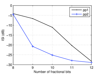
Figure 1: ISI vs number of fractional bits comparison between two post-processing techniques for CO-CMA for SISO channel, 16 QAM signal (SNR=$18$dB, $K=1000$, $L_{\text{w}}=5$)

Figure 1 compares the residual ISI of the two aforementioned methods averaged over $500$ Monte Carlo runs. As figure 1 reveals, pp2 outperforms pp1 when the number of fractional bits are from 9 to 11. It is clear that when the number of fractional bits is not sufficient, the small values become zeros and the pp1 suffers from division by zero problem. In contrast, the pp2 does not have the normalization step as in pp1 making pp2 more robust for fixed point implementation.

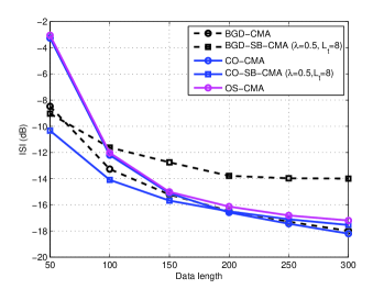
Figure 2: ISI performance of different blind/semiblind algorithms using convex optimization for the SISO channel with $4$-QAM input (SNR=$8$dB).

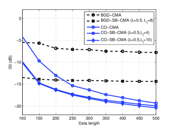
Figure 3: ISI performance of different blind/semiblind algorithms using convex optimization for the SISO channel with $16$ QAM input (SNR=$14$dB).

To assert the behavior of the convex optimization algorithms, we test the algorithms on the fix channel in (63). In the rest of simulation results, for convex optimization, only the proposed post-processing technique with floating point is used. The equalizer length is $6$. Figures 2 and 3 show the ISI performance of the semiblind algorithms for the SISO channel with QPSK and 16-QAM signals, respectively, when data length $K$ varies. The SNR in QPSK system is 8 dB and in 16-QAM system is 14 dB, For semiblind algorithms, $\lambda=0.5$ and $L_{\text{t}}=8$. For BGD algorithms, the initialization is $[0\;0\;1\;0\;0\;0]$. For good ISI performance, the step size is set at $0.01$ and $0.001$ for QPSK and 16-QAM, respectively. With QPSK inputs, the blind algorithms have almost the same performance for a large enough $K$. It is known that the channel is fairly easy to equalize and with the initialization, the BGD actually converges to the global minima. The performance of semiblind algorithms are worse than that of the corresponding blind ones. It is expectable since the pilots may deviate the semiblind costs from a good result due to the instantaneous noise value on the pilots [34]. With 16-QAM inputs, the blind cost appears to have many local minima and the BGD-CMA cannot converge to good local minima even when the data length is considered sufficient. The pilots help the BGD-SB-CMA to eliminate many unsatisfactory local minima. However, it still cannot achieve global minimum. On the other hand, the CO-CMA and the CO-SB-CMA have substantially better performance than the BGD counterpart. Comparing the CO-CMA and the CO-SB-CMA for large $K$, i.e., $K$=500, we can see that the performance difference is negligible even when we increase the pilot length. This indicates that the CO-CMA converge to global minimum. For smaller $K$, as $K$ decreases, the performance of all the convex optimization based algorithms degrade since the estimation of the statistics become less accurate. With only a few pilot symbols, the SB-CO-CMA reduces ISI substantially, especially when the data length is small.

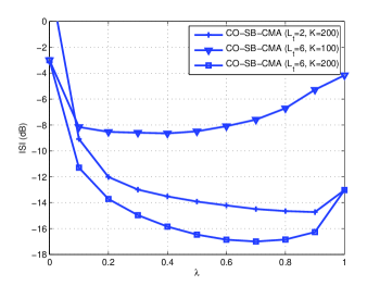
Figure 4: ISI vs weighting factor $\lambda$ for CO-SB-CMA for SISO channel and 16-QAM input (SNR=$14$dB).

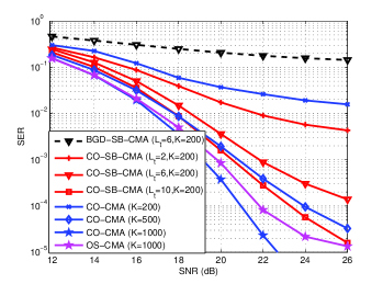
Figure 5: SER vs SNR comparison between CMA and the SB-CMA using convex optimization (SISO channel, 16 QAM signal).

We also compare the CO-CMA and the optimal stepsize CMA algorithm in [34] and [18] (marked as "OS-CMA"). For the chosen simulation parameter set, the CO-CMA outperforms the OS-CMA slightly.

Figure 4 shows the ISI versus $\lambda$ of the SB-CO-CMA for several setups. The semiblind algorithm always outperforms the blind counterpart and the training based one. The result also indicates that the weighting factor must be carefully chosen . The optimum weight depends on the choice of the length of training symbols and the length of available data.

Figure 5 shows the symbol error rate (SER) versus SNR performance for the blind and semiblind algorithms using convex optimization under 16-QAM signal. We can see that the CO algorithms improve the performance significantly when comparing with the BGD algorithm. Figure 5 also confirms that with the help of a few pilot symbols, the semiblind algorithms significantly reduce the need for long data sequence. In particular, with only $6$ or $10$ pilot symbols, the data length $K$ for the SB algorithm is only $200$ compare to $500$ for the blind algorithm. Therefore, the CO processing technique is suitable for short burst data transmission. Compared to OS-CMA, the performance of CO-CMA is significant better. This is because the cost for 16-QAM appears to have many local minima and OS-CMA does not guarantee to converge to the global one.

VII-B Blind source separation problem

In this part, we investigate the source separation ability of the new algorithms. We test the algorithms on a $4\times 4$ mixing matrix for source separation problem. In this case, by limiting $k=0$ in the performance metric in (60), we define the measure metric as the calculated normalized cross-channel interference (NCCI) for source $i$.

$$\text{NCCI}_{i}=\frac{\sum_{j}\left|c_{i,j}\right|^{2}-\text{max}_{j}\left|c_{i,j}\right|^{2}}{\text{max}_{j}\left|c_{i,j}\right|^{2}}.$$ (64)

In the following simulation results, we use the average NCCI of all the combined channels to compare different simulation setups.

In our example, the mixing matrix $\mathbf{H}$ is $4\times 4$ with entries

$$\mathbf{H} \!\!=\!\!\!\left[\begin{array}[]{cccc}\!\!\!0.41+0.05j&\!\!\!\!\!\!0.45+0.62j&\!\!\!0.26+0.92j&\!\!-0.25-0.61j\\ \!\!\!0.52-1.11j&\!\!\!\!\!1.04-0.12j&\!\!\!0.06+0.66j&\!\!-0.81+0.21j\\ \!\!\!0.07-0.80j&\!\!\!\!1.30+0.33j&\!\!\!1.40+0.65j&\!\!-0.05+0.94j\\ \!\!\!0.47-1.08j&\!\!\!0.83+0.43j&\!\!\!0.94-0.08j&\!\!0.57+0.19j\end{array}\!\!\!\!\right]$$

Each of the 4 channel outputs has AWG noise with SNR of $10$dB. We apply the CMA algorithms without cross-cumulant jointly with the Gram-Schmidt orthogonalization process to separate different sources [35]. For BGD algorithms, the initial values for $\{\mathbf{w}_{i},\;i=1,2,3,4\}$ are $\left[1\>0\>0\>0\right]^{T}$, $\left[0\>1\>0\>0\right]^{T}$, $\left[0\>0\>1\>0\right]^{T}$, $\left[0\>0\>0\>1\right]^{T}$. The step size is set at $10^{-3}$ for $4$-QAM and $10^{-5}$ for $16$-QAM signals and the update iterations are long enough for the best NCCI performance. For the semiblind algorithm, the pilot for each data stream is chosen orthogonal. Although the training symbols can do the source separation task, we still use the cross correlation cost as the semiblind cost for the second channel given by $J_{\text{sb},2}=(1-\lambda)J_{\text{t},2}+\lambda J_{\text{b},2}+\lambda_{\text{cr}}J_{\text{cr},2,1}$ with $\lambda_{\text{cr}}=1$. If $\lambda=1$, the semiblind algorithms reduce to the blind algorithms. This semiblind cost is also used in the simulation for MIMO channel.

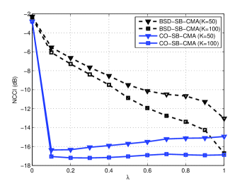
Figure 6: NCCI vs weighting factor for the mixing matrix with QPSK signals ($L_{t}=4)$.

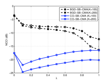
Figure 7: NCCI vs weighting factor for the mixing matrix with 16-QAM signal ($L_{t}=4)$.

Figures 6 and 7 compare the NCCI between the semiblind algorithms using CMA cost when the channel inputs are $4$-QAM and $16$-QAM, respectively. The solutions are achieved by the proposed convex optimization or by the BGD. For the BGD the pilot cost is the linear least square (LS) cost which is commonly used. We can see that for short data length, the convex optimization approach outperforms the BGD one. In this scenario, few pilots do not help to improve the performance of BGD. In addition, it creates undesired local minima that the BGD may converge to. Meanwhile, despite of the bad local minima, the performance of the CO-SB-CMA is superior to the BGD algorithms. For 16-QAM, the NCCI is lower as the $\lambda$ is decreased. This implies that for few observations ($K=100,200)$ the estimation of high-order statistics is not accurate and the semiblind algorithms rely on pilots to achieve good performance. For QPSK case, we observe the same behavior although the performance difference between the CO-SB-CMA and the CO-CMA is smaller.

Observing figures 6 and 7, we notice an interesting phenomenon about the pilot based costs. When $\lambda=1$, the SB-BGD-CMA cost reduces to the linear least square cost. If the pilot length is short compared with the equalizer length, as the algorithm converges, over fitting problem occurs. It is because in the LS cost there are only $L_{\text{t}}$ square terms. Meanwhile, for the SB-CO-CMA, the fourth order pilot cost has $L_{\text{t}}(L_{\text{t}}-1)/2$ square terms making this cost more resilient to the overfitting problem. That is the reason why even with only a few pilot symbols, the fourth order cost outperforms the LS cost. We also notice that this performance gap is more significant for $16$-QAM input. This phenomenon may need further analysis.

VII-C MIMO channel

TABLE III: The $2\times 2$ MIMO channel coefficients ( $L_{h}=2$)

$k$	$h_{1,1}\left(k\right)$	$h_{1,2}\left(k\right)$	$h_{2,1}\left(k\right)$	$h_{2,2}\left(k\right)$
0	$-0.2+0.1j$	$.1j$	$0.1j$	$1$
1	$1$	$0.2$	$0.1$	$0.1j$
2	$0.2j$	$0.11$	$0.2j$	$0.1+0.1j$

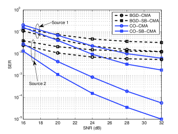
Figure 8: SER vs SNR comparison between CMA and the SB-CMA using convex optimization for MIMO channel, 16 QAM signal ($K=500$, $L_{\text{t}}=4$)

In this test, we apply our CO approaches using CMA and SB-CMA on a MIMO channel. We consider a $2\times 2$ FIR channel whose coefficients are shown in Table III. The signal inputs are 16-QAM and the additive white Gaussian noise is added to form channel outputs. For each sub-channel, an FIR equalizer of order $L_{w}=3$ is applied. We choose orthogonal pilot sequences of length $L_{\text{t}}=4$ symbols each. The weighting factor $\lambda=0.5$ for SB algorithms is considered. We compare the CO algorithms with the BGD algorithms. The stepsize for the BGD is optimized to achieve minimum ISI. The initial coefficient set is single unit spike at its near-center tap for $\mathbf{w}_{i,i}$ and zeros otherwise:

$$\mathbf{w}_{i,j} = \begin{cases}[0\;1\;0\;0]^{T}&\text{for }i=j,\\ {}[0\;0\;0\;0]^{T}&\text{for }i\neq j.\end{cases}$$ (65)

Figure 8 compares SER performance of BGD and CO implementations as functions of SNR for CMA and SB-CMA equalizer for each data source. The results confirm that the CO implementation also outperforms the BGD in MIMO scenario. Similar to SISO and source separation scenarios, with only a few pilot symbols, the CO-SB-CMA equalization achieves better performance over the CO-CMA equalization.

VIII Conclusions

We formulated various blind channel equalization and source separation costs utilizing only fourth order and second order statistics into convex semi-definite optimization using real-valued data and parameters. Compared to the precedent work in [21], our formulation is more compact and resource saving, thereby, more efficient. We also proposed a post-processing technique that is more suitable in practice. Our formulation can be applied for signals of high-order QAM constellation in general MIMO systems. The global solution is found without requirement of having good initialization as the conventional implementation using gradient descent method. The number of data required for successfully equalizing the channels or separating sources is low compared to other batch algorithms making this method suitable for short packet transmission under fast fading channels. We also proposed a fourth order training based cost and form semi-blind algorithms. Using only a few pilot symbols, the semi-blind algorithms outperform the blind cost counterpart and other semi-blind algorithms.

Appendix A

In this appendix, we provide detail calculation for the cross-correlation term $J_{\text{cr},i,j}$. Note that, $\mathbf{w}_{i}$ for $i<j$ is already known. First, we calculate the cross-correlation as a function of $\mathbf{v}_{j}=\mbox{qvec}\left(\mathbf{u}_{j}\right)$. Now

$$\left|E\left[y_{i}\left(k\right)y_{j}^{*}\left(k-l\right)\right]\right|^{2} =\left|E\left[\mathbf{w}_{i}^{H}\mathbf{x}\left(k\right)\mathbf{x}^{H}\left(k-l\right)\mathbf{w}_{j}\right]\right|^{2}$$

$$=\left|\mathbf{w}_{i}^{H}E\left[\mathbf{x}\left(k\right)\mathbf{x}^{H}\left(k-l\right)\right]\mathbf{w}_{j}\right|^{2}.$$ (66)

Since $\mathbf{w}_{i}$ is known, we can pre-calculate $\mathbf{p}_{i,l}=\left(\mathbf{w}_{i}^{H}E\left[\mathbf{x}\left(k\right)\mathbf{x}^{H}\left(k-l\right)\right]\right)^{H}$. Let

$$\mathbf{p}_{\text{r},i,l} =\left[\begin{array}[]{cc}\text{Re}\left\{\mathbf{p}_{i,l}^{T}\right\}&\text{Im}\left\{\mathbf{p}_{i,l}^{T}\right\}\end{array}\right]^{T},$$

$$\mathbf{p}_{\text{i},i,l}^{T} =\left[\begin{array}[]{cc}\text{Im}\left\{\mathbf{p}_{i,l}^{T}\right\}&-\text{Re}\left\{\mathbf{p}_{i,l}^{T}\right\}\end{array}\right]^{T},$$

we have

$$\left|E\left[y_{i}\left(k\right)y_{j}^{*}\left(k-l\right)\right]\right|^{2} =\left|\mathbf{p}_{i,l}^{H}\mathbf{w}_{j}\right|^{2}$$

$$=\mathbf{u}_{j}^{T}\left(\mathbf{p}_{\text{r},i,l}\mathbf{p}_{\text{r},i,l}^{T}+\mathbf{p}_{\text{i},i,l}\mathbf{p}_{\text{i},i,l}^{T}\right)\mathbf{u}_{j}$$

$$=\mathbf{q}_{i,l}^{T}\mathbf{v}_{j}$$ (67)

with $\mathbf{q}_{i,l}=\mbox{svec}\left(\mathbf{p}_{\text{r},i,l}\mathbf{p}_{\text{r},i,l}^{T}+\mathbf{p}_{\text{i},i,l}\mathbf{p}_{\text{i},i,l}^{T}\right)$. Therefore

$$\sum_{i=1}^{j-1}J_{\text{cr},i,j} =\sum_{i=1}^{j-1}\sum_{l=0}^{\delta}\mathbf{q}_{i,l}^{T}\mathbf{v}_{j}$$

$$=\mathbf{q}_{j}^{T}\mathbf{v}_{j}$$ (68)

where $\displaystyle\mathbf{q}_{j}=\sum_{i=1}^{j-1}\sum_{l=0}^{\delta}\mathbf{q}_{i,l}.$

Appendix B

In this appendix, we present the details of calculation for $\mathbf{C}_{\text{t}}$, $\mathbf{b}_{\text{t}}$, $a_{\text{t}}$ in Section V.

Since

$$\mathbf{u}^{T}\mathbf{x}_{\text{t}}(p)\mathbf{x}_{\text{t}}^{T}(q)\mathbf{u} =\mathbf{u}^{T}\mathbf{x}_{\text{t}}(q)\mathbf{x}_{\text{t}}^{T}(p)\mathbf{u}$$

$$=\mathbf{u}^{T}\left[\frac{\mathbf{x}_{\text{t}}(p)\mathbf{x}_{\text{t}}^{T}(q)}{2}+\frac{\mathbf{x}_{\text{t}}(q)\mathbf{x}_{\text{t}}^{T}(p)}{2}\right]\mathbf{u},$$

we can write

$$J_{\text{t}}=\sum_{p=1}^{2L_{\text{t}}}\sum_{q=p}^{2L_{\text{t}}}\left[\mathcal{X}^{T}(p,q)\mathbf{v}-s_{\text{t}}(p)s_{\text{t}}(q)\right]^{2}$$ (69)

where $\mathcal{X}(p,q)=\mbox{svec}\left(\frac{\mathbf{x}_{\text{t}}(p)\mathbf{x}_{\text{t}}^{T}(q)}{2}+\frac{\mathbf{x}_{\text{t}}(q)\mathbf{x}_{\text{t}}^{T}(p)}{2}\right)$.

The cost can be written as the second order function of $\mathbf{v}$:

$$J_{\text{t}} =\sum_{p=1}^{2L_{\text{t}}}\sum_{q=p}^{2L_{\text{t}}}\mathbf{v}^{T}\mathcal{X}(p,q)\mathcal{X}^{T}(p,q)\mathbf{v}$$ (70)

$$-\sum_{p=1}^{2L_{\text{t}}}\sum_{q=p}^{2L_{\text{t}}}2s_{\text{t}}(p)s_{\text{t}}(q)\mathcal{X}^{T}(p,q)\mathbf{v}+\sum_{p=1}^{2L_{\text{t}}}\sum_{q=p}^{2L_{\text{t}}}s_{\text{t}}(p)s_{\text{t}}(q)$$

$$=\mathbf{v}^{T}\mathbf{C}_{\text{t}}\mathbf{v}-\mathbf{b}_{\text{t}}\mathbf{v}+a_{\text{t}}$$ (71)

where

$$\mathbf{C}_{\text{t}}=\sum_{p=1}^{2L_{\text{t}}}\sum_{q=p}^{2L_{\text{t}}}\mathcal{X}(p,q)\mathcal{X}^{T}(p,q),$$ (72)

$$\mathbf{b}_{\text{t}}=\sum_{p=1}^{2L_{\text{t}}}\sum_{q=p}^{2L_{\text{t}}}2s_{\text{t}}(p)s_{\text{t}}(q)\mathcal{X}^{T}(p,q),$$ (73)

$$a_{\text{t}}=\sum_{p=1}^{2L_{\text{t}}}\sum_{q=p}^{2L_{\text{t}}}s_{\text{t}}(p)s_{\text{t}}(q).$$ (74)

Huy-Dung Han Huy-Dung Han received B.S. in 2001 from Faculty of Electronics and Telecommunications at Hanoi University of Science and Technology, Vietnam, M. Sc. degree in 2005 from Technical Faculty at University Kiel, Germany and Ph.D. degree in 2012, from the Department of Electrical and Computer Engineering at the University of California, Davis, USA. His research interests are in the area of wireless communications and signal processing, with current emphasis on blind and semi-blind channel equalization for single and multi-carrier communication systems, convex optimization. Dr. Han is with School of Electronics and Telecommunications, Department of Electronics and Computer Engineering at Hanoi University of Science and Technology, Hanoi, Vietnam. He has been serving on technical programs of IEEE International Conference on Communications and Electronics.

Muhammad Zia Muhammad Zia received M. Sc. degree in 1991 and M.Phil degree in 1999, both from Department of Electronics at Quaid-e-Azam University, Islamabad, Pakistan. He received PhD degree from the Department of Electrical and Computer Engineering at the University of California, Davis in 2010. His research interests are in the area of wireless communications and signal processing, with current emphasis on the wireless security, compressive sensing, bandwidth efficient transceiver design and blind and semi-blind detection of Space-Time Block Codes. Dr. Zia is with Department of Electronics at Quaid-i-Azam University, Islamabad.

Zhi Ding Zhi Ding (S’88-M’90-SM’95-F’03) is Professor of Electrical and Computer Engineering at the University of California, Davis. He received his Ph.D. degree in Electrical Engineering from Cornell University in 1990. From 1990 to 2000, he was a faculty member of Auburn University and later, University of Iowa. Prof. Ding has held visiting positions in Australian National University, Hong Kong University of Science and Technology, NASA Lewis Research Center and USAF Wright Laboratory. Prof. Ding has active collaboration with researchers from areas including Australia, China, Japan, Canada, Finland, Taiwan, Korea, Singapore, and Hong Kong. Dr. Ding is a Fellow of IEEE and has been an active volunteer, serving on technical programs of several workshops and conferences. He was associate editor for IEEE Transactions on Signal Processing from 1994-1997, 2001-2004, and associate editor of IEEE Signal Processing Letters 2002-2005. He was a member of technical committee on Statistical Signal and Array Processing and member of Technical Committee on Signal Processing for Communications (1994-2003). Dr. Ding was the Technical Program Chair of the 2006 IEEE Globecom. He was also an IEEE Distinguished Lecturer (Circuits and Systems Society, 2004-06, Communications Society, 2008-09). He served on as IEEE Transactions on Wireless Communications Steering Committee Member (2007-2009) and its Chair (2009-2010). Dr. Ding received the 2012 IEEE Wireless Communication Recognition Award from the IEEE Communications Society and is a coauthor of the text: Modern Digital and Analog Communication Systems, 4th edition, Oxford University Press, 2009.

References

- [1] Cable Television Laboratories Inc., “Proactive network maintenance using pre-equalization,” no. CM-GL-PNMP-V01-100415, 2010.
- [2] J. Johnson, C. R., P. Schniter, T. J. Endres, J. D. Behm, D. R. Brown, and R. A. Casas, “Blind equalization using the constant modulus criterion: a review,” Proc. IEEE, vol. 86, no. 10, pp. 1927–1950, 1998.
- [3] Y.-S. Choi, D. S. Han, and H. Hwang, “Joint blind equalization, carrier recovery, and timing recovery for HDTV modem,” in Society of Photo-Optical Instrumentation Engineers (SPIE) Conference Series, B. G. Haskell & H.-M. Hang, Ed., vol. 2094, Oct. 1993, pp. 1357–1365.
- [4] J.-J. Werner, J. Yang, D. D. Harman, and G. A. Dumont, “Blind equalization for broadband access,” IEEE Commun. Mag., vol. 37, no. 4, pp. 87–93, 1999.
- [5] Z. Ding and Z.-Q. Luo, “A fast linear programming algorithm for blind equalization,” IEEE Trans. Commun., vol. 48, no. 9, pp. 1432–1436, 2000.
- [6] M. Muhammad and Z. Ding, “A linear programming receiver for blind detection of full rate space-time block codes,” IEEE Trans. Signal Process., vol. 58, no. 11, pp. 5819–5834, 2010.
- [7] D. N. Godard, “Self-recovering equalization carrier tracking in two dimensional data communications systems,” IEEE Trans. Commun., vol. 28, pp. 1867–1875, Nov. 1980.
- [8] J. Treichler and B. Agee, “A new approach to multipath correction of constant modulus signals,” IEEE Trans. Acoust., Speech, Signal Process., vol. 31, no. 2, pp. 459–472, Apr. 1983.
- [9] O. Shalvi and E. Weinstein, “New criteria for blind deconvolution of nonminimum phase systems (channels),” IEEE Trans. Inf. Theory, vol. 36, no. 2, pp. 312–321, 1990.
- [10] R. A. Wiggins, “Minimum entropy deconvolution,” Geoexploration, vol. 16, pp. 21–35, 1978.
- [11] D. L. Donoho, “On minimum entropy deconvolution,” Applied Time Series Analysis, II., 1981.
- [12] R. A. Kennedy, B. D. O. Anderson, Z. Ding, and J. Johnson, C. R., “Local stable minima of the sato recursive identification scheme,” in Proc. 29th IEEE Conf. Decision and Control, 1990, pp. 3194–3199.
- [13] T.-H. Li, “Blind deconvolution of linear systems with multilevel nonstationary inputs,” The Annals of Statistics, vol. 23, no. 2, pp. 690–704, Apr 1995.
- [14] B. Agee, “The least-squares CMA: A new technique for rapid correction of constant modulus signals,” in Proc. IEEE International Conference on ICASSP ’86. Acoustics, Speech, and Signal Processing, vol. 11, Apr. 1986, pp. 953–956.
- [15] R. Pickholtz and K. Elbarbary, “The recursive constant modulus algorithm; a new approach for real-time array processing,” in Conference Record of The Twenty-Seventh Asilomar Conference on Signals, Systems and Computers, Nov. 1–3, 1993, pp. 627–632.
- [16] P. A. Regalia, “A finite-interval constant modulus algorithm,” in Proc. IEEE International Conference on Acoustics, Speech, and Signal Processing (ICASSP ’02), vol. 3, May 13–17, 2002, pp. III–2285–III–2288.
- [17] Y. Chen, T. Le-Ngoc, B. Champagne, and C. Xu, “Recursive least squares constant modulus algorithm for blind adaptive array,” IEEE Trans. Signal Process., vol. 52, no. 5, pp. 1452–1456, May 2004.
- [18] V. Zarzoso and P. Comon, “Optimal step-size constant modulus algorithm,” IEEE Trans. Commun., vol. 56, no. 1, pp. 10–13, Jan. 2008.
- [19] E. Satorius and J. Mulligan, “An alternative methodology for blind equalization,” Digital Signal Processing: A Review Journal, vol. 3, pp. 199–209, 1993.
- [20] K. Dogancay and R. A. Kennedy, “Least squares approach to blind channel equalization,” IEEE Trans. Commun., vol. 47, no. 11, pp. 1678–1687, 1999.
- [21] B. Maricic, Z.-Q. Luo, and T. N. Davidson, “Blind constant modulus equalization via convex optimization,” IEEE Trans. Signal Process., vol. 51, no. 3, pp. 805–818, 2003.
- [22] H.-D. Han, Z. Ding, J. Hu, and D. Qian, “On steepest descent adaptation: A novel batch implementation of blind equalization algorithms,” in Proc. IEEE Global Telecommunications Conf. GLOBECOM 2010, 2010, pp. 1–6.
- [23] C. B. Papadias and A. J. Paulraj, “A constant modulus algorithm for multiuser signal separation in presence of delay spread using antenna arrays,” IEEE Signal Process. Lett., vol. 4, no. 6, pp. 178–181, 1997.
- [24] Y. Li and K. J. R. Liu, “Adaptive blind source separation and equalization for multiple-input/multiple-output systems,” IEEE Trans. Inf. Theory, vol. 44, no. 7, pp. 2864–2876, Nov. 1998.
- [25] N. Z. Shor and P. I. Stetsyuk, “The use of a modification of the r-algorithm for finding the global minimum of polynomial functions,” Cybernetics and Systems Analysis, vol. 33, pp. 482–497, 1997.
- [26] P. A. Parrilo, “Structured semidefinite programs and semialgebraic geometry methods in robustness and optimization,” Ph.D. dissertation, California Institute of Technology, May 2000, available at http://www.cds.caltech.edu/ pablo/.
- [27] Y. Nesterov, High Performance Optimization. Boston, MA:: Kluwer, 2000, ch. Squared functional systems and optimization problems, pp. 405–440.
- [28] L. Vandenberghe and S. Boyd, “Semidefinite programming,” SIAM Review, vol. 38, no. 1, pp. 49–95, 1996.
- [29] P. A. Parrilo and B. Sturmfels, “Minimizing polynomial functions,” Algorithmic and quantitative real algebraic geometry, DIMACS Series in Discrete Mathematics and Theoretical Computer Science, vol. 60, pp. 83–99, 2003.
- [30] W. Rudin, “Sums of squares of polynomials,” The American Mathematical Monthly, vol. 107, no. 9, pp. 813–821, 11 2000.
- [31] R. Tutuncu, K. Toh, and M. Todd, “Solving semidefinite-quadratic-linear programs using SDPT3,” Mathematical Programming Ser. B, vol. 95, pp. 189–217, 2003.
- [32] Z. Ding and Y. Li, Blind equalization and identification. CRC, 2001.
- [33] Y. Chen, C. Nikias, and J. G. Proakis, “CRIMNO: criterion with memory nonlinearity for blind equalization,” in Conference Record of the Twenty-Fifth Asilomar Conference on Signals, Systems and Computers, Nov. 4–6, 1991, pp. 694–698.
- [34] V. Zarzoso and P. Comon, “Semi-blind constant modulus equalization with optimal step size,” in Proc. IEEE Int. Conf. Acoustics, Speech, and Signal Processing (ICASSP ’05), vol. 3, 2005.
- [35] Z. Ding and T. Nguyen, “Stationary points of a kurtosis maximization algorithm for blind signal separation and antenna beamforming,” IEEE Trans. Signal Process., vol. 48, no. 6, pp. 1587–1596, 2000.