Local Operators in Kinetic Wealth Distribution

Abstract

The statistical mechanics approach to wealth distribution is based on the conservative kinetic multi-agent model for money exchange, where the local interaction rule between the agents is analogous to the elastic particle scattering process. Here, we discuss the role of a class of conservative local operators, and we show that, depending on the values of their parameters, they can be used to generate all the relevant distributions. We also show numerically that in order to generate the power-law tail an heterogeneous risk aversion model is required. By changing the parameters of these operators one can also fine tune the resulting distributions in order to provide support for the emergence of a more egalitarian wealth distribution.

Calgary, Alberta, T3G 5Y8, Canada

mircea.andrecut@gmail.com

1 Introduction

More than a century ago, Pareto has noticed that the wealth distribution in a stable economy seems to follow a power law distribution:

$$F(w)=\int_{w}^{\infty}f(w)dw\propto w^{-\nu}.$$ (1)

where $F(w)$ is the cumulative probability of individuals with a wealth of at least $w$, and $f(w)$ is the probability distribution function [1]. This power law, and the index $\nu$ are known today as Pareto law, and respectively Pareto index.

Further studies have shown that Pareto’s law only explains the distribution of the higher income class, situated on the tail of the wealth distribution. Away from the tail, the distribution is better described by a Gamma or Log-normal distribution known as Gibrat’s law [2]. More recent studies also suggest that the low income class can be described by Boltzmann-Gibbs and Gamma-like distributions $f_{G}(w)$ [3, 4, 5, 6, 7, 8, 9, 10]:

$$f(w) \propto\begin{cases}f_{G}(w)&\text{for }w<w_{c}\\ w^{-\nu-1}&\text{for }w\geq w_{c}\end{cases}.$$ (2)

These recent studies show that the Pareto law with an index $\nu\in[1,2]$, with slight variations, exhibits a remarkable stability in the real data, showing that a small percentage of people are holding the majority of wealth.

Several multi-agent models of closed economies have been proposed to explain these empirical results (for a review see [11] and the references therein). These models borrow methods from the statistical mechanics of particle systems, and their basic assumption is that wealth is exchanged among agents at a microscopic level, using a simple pairwise trade mechanism, which is physically equivalent to a particle scattering process [12]. Despite their simplicity, these models exhibit the characteristics of real data and provide a framework for better understanding the complexity behind the wealth distribution mechanism.

Most of these models are based on conservative microscopic interactions, and have focused on incorporating a saving mechanism, which allows only a fraction of the agent’s wealth to participate in each trading event [13, 14]. More recently, effort was made to include macroscopic mechanisms for global taxation and wealth redistribution in an effort to counter the concentration of all available wealth in few agents, and to favour the poorer agents [15]. These mechanisms can also lead to the creation of a middle class, since the models implementing them exhibit a transition from the "unfair" Boltzmann-Gibbs distribution to a Gamma-like unimodal distribution, where most of the agent’s wealth is shifted away from zero to a positive value, corresponding to the mode of the distribution.

Here, we discuss the role of a class of conservative local operators, and we show that, depending on the values of their parameters, they can be used to generate all the relevant wealth distributions: Dirac delta, Boltzmann-Gibbs, Gamma and Pareto. We also show numerically that in order to generate the power-law tail an heterogeneous risk aversion model is required. By changing the parameters of these operators one can also fine tune the resulting distributions in order to provide support for the emergence of a more egalitarian wealth distribution.

2 Kinetic models for wealth distribution

While wealth is a complex concept that includes money, property and other material goods that have a certain economic utility, here we consider that wealth is measured only in terms of money. We also assume that money is the exchange medium used in economic transactions between agents, and that the total amount of money is a conserved quantity in a closed economy.

We consider a closed economy with $N$ agents, characterized by their wealth state $w_{n}\geq 0$, $n=1,2,...,N$. The economic transactions are described as binary interactions, where at a given time step, two random agents $i$ and $j$ are exchanging an amount of wealth (money) $\Delta w$ between them:

$$w^{\prime}_{i} =w_{i}-\Delta w,$$

$$w^{\prime}_{j} =w_{j}+\Delta w,$$ (3)

such that total amount of money of the two agents, before and after transaction, is conserved:

$$w^{\prime}_{i}+w^{\prime}_{j}=w_{i}+w_{j}.$$ (4)

This local conservation law for money is analogous to the energy conservation in the elastic collisions between the molecules of an ideal gas.

In the most closely related model to traditional statistical mechanics the transaction wealth exchange quantity is defined as:

$$\Delta w=(1-\eta)w_{i}-\eta w_{j},$$ (5)

such that the local transaction equations are:

$$w^{\prime}_{i} =\eta(w_{i}+w_{j}),$$

$$w^{\prime}_{j} =(1-\eta)(w_{i}+w_{j}),$$ (6)

where $\eta\sim U[0,1]$ is a uniform distributed random variable, governing the random redistribution of the wealth of the agents [11]. It has been shown that this basic model leads to an equilibrium Boltzmann-Gibbs distribution:

$$f(w)=\frac{1}{\langle w\rangle}\exp\left(-\frac{w}{\langle w\rangle}\right),$$ (7)

with the "temperature" equal to the average amount of money per agent $\langle w\rangle$ [12]. This result is extremely robust and independent of various factors, such as arbitrary initial conditions and random or consecutive interaction of agents. The Boltzmann-Gibbs distribution is characterized by very few rich agents and a majority of poor agents, without a well defined middle class.

In order to overcome the "unfairness" of the Boltzmann-Gibbs wealth distribution, one can include a savings mechanism that leads to a more "fair" Gamma-like equilibrium distribution [13]. In this case the agents save some fraction of their money $\lambda w_{i}$, and use the rest of their money balance, $(1-\lambda)w_{i}$, for random exchanges, such that the locally conservative transaction equations become:

$$w^{\prime}_{i} =\lambda w_{i}+\eta(1-\lambda)(w_{i}+w_{j}),$$

$$w^{\prime}_{j} =\lambda w_{j}+(1-\eta)(1-\lambda)(w_{i}+w_{j}).$$ (8)

The coefficient $\lambda\in[0,1]$ is a global constant called the saving propensity. It was also shown that the equilibrium distribution of this model is close to a Gamma distribution [13].

A further enhancement of this model considers different saving propensities for the agents.[14] The propensities also maintain their values fixed during the relaxation dynamics of the system. It was found that this model produces a Gamma-like distribution ending with a Pareto tail with an index $\nu\simeq 1$, which originates from the agents with a saving propensity close to one [14].

A different approach considers a macroscopic mechanism for global taxation and wealth redistribution which favours the poorer agents [15]. In such a model, any transaction can be described in two steps. In the first step, two random agents $i$ and $j$ exchange their money such that a fraction $f\in[0,1)$ of their exchanged wealth is lost by taxes:

$$w_{i}(t+1/2) =(1-f)\eta[w_{i}(t)+w_{j}(t)],$$

$$w_{j}(t+1/2) =(1-f)(1-\eta)[w_{i}(t)+w_{j}(t)].$$ (9)

In the second step, the collected taxes $\tau=f[w_{i}(t)+w_{j}(t)]$ are equally redistributed to all the agents in the population:

$$w_{n}(t+1)=w_{n}(t+1/2)+\tau/N,\>n=1,...,N.$$ (10)

The transactions can be described by inelastic collisions between gas particles, where the energy lost is the analogue of the taxation value. The model exhibits a transition from the Boltzmann-Gibbs distribution to a Gamma-like distribution as $f$ increases, and after a critical point it returns to an exponential for higher $f$ values.

3 Local operators in kinetic wealth distribution

Here we discuss the role of a class of conservative local operators in the wealth exchange dynamics. Also, in order to characterize the wealth distributions we use the mode of the distribution, when it is present, and the Gini coefficient, which measures the inequality among the values in the distribution [16]. A Gini coefficient $G=1$ expresses the maximal wealth inequality, while a Gini coefficient $G=0$ corresponds to perfect equality, where all the wealth values are the same. For a population $w_{n}\geq 0$, $n=1,2,...,N$, that is indexed in non-decreasing order ($w_{n}\leq w_{n+1}$), the Gini coefficient can be easily computed as following [17, 18]:

$$G=\frac{1}{N}\left[N+1-2\frac{\sum_{n=1}^{N}(N+1-n)w_{n}}{\sum_{n=1}^{N}w_{n}}\right]$$ (11)

Also, in all the computations we impose a conserved total wealth:

$$W=\sum_{n=1}^{N}w_{n}=N$$ (12)

Let us first consider the basic model described by the equation (6), written in the following matrix form:

$$\begin{bmatrix}w_{i}(t+1)\\ w_{j}(t+1)\end{bmatrix}=T^{+}(\varepsilon)\begin{bmatrix}w_{i}(t)\\ w_{j}(t)\end{bmatrix}$$ (13)

where

$$T^{+}(\varepsilon)=\begin{bmatrix}\varepsilon&\varepsilon\\ 1-\varepsilon&1-\varepsilon\end{bmatrix}$$ (14)

and $\varepsilon\sim U[0,1]$ is an uniformly distributed random variable. One can see that this is a stochastic operator corresponding to a column stochastic matrix, which is also singular, and therefore non-invertible. It is interesting to note that $T^{+}(\varepsilon)$ has no memory of its previous applications:

$$T^{+}(\varepsilon)T^{+}(\varepsilon^{\prime})=T^{+}(\varepsilon),\>\>\forall\varepsilon^{\prime}\neq\varepsilon$$ (15)

which means that the result of its successive applications only depends on the last application [19]. Also, it is well known that starting from any distribution of money, and by applying this local interaction rule, the steady state of the wealth distribution becomes a Boltzmann-Gibbs distribution [12].

Let us now replace the $T^{+}(\varepsilon)$ operator in this basic model with the following operator:

$$T^{-}(\varepsilon)=\begin{bmatrix}\varepsilon&1-\varepsilon\\ 1-\varepsilon&\varepsilon\end{bmatrix}$$ (16)

where $\varepsilon\sim U[0,1]$. This operator corresponds to a non-singular double stochastic matrix, which is not memoryless, since its successive applications accumulate as follows:

$$T^{-}(\varepsilon)T^{-}(\varepsilon^{\prime})=T^{-}(\varepsilon^{\prime\prime})$$

$$T^{-}(\varepsilon)T^{+}(\varepsilon^{\prime})=T^{+}(\varepsilon^{\prime\prime})$$ (17)

where $\varepsilon^{\prime\prime}=\varepsilon\varepsilon^{\prime}+(1-\varepsilon)(1-\varepsilon^{\prime})$.

Figure 1: Time evolution of a uniform wealth distribution into a Dirac delta function (left) and a Boltzmann-Gibbs distribution (right), using the $T^{-}(\varepsilon)$ and respectively $T^{+}(\varepsilon)$ operators.

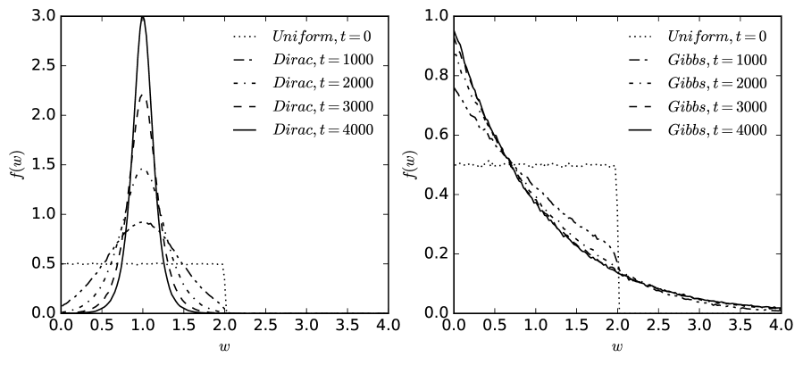
Our numerical simulations show that by applying this local interaction rule, the steady state of any wealth distribution becomes a Dirac delta function, independent of the initial distribution. In Figure 1 we show such a simulation, where a population of $N=1000$ agents with an initial wealth $W=N$, uniformly distributed among them in $U[0,2]$ with an average $\langle w\rangle=1$, is evolved to either a Dirac delta function (Fig.1, left), or a Boltzmann-Gibbs distribution (Fig.1, right). During the numerical simulation, a pair of agents is randomly drawn at every time step, and they interact locally using the $T^{-}(\varepsilon)$ or $T^{+}(\varepsilon)$ operators, respectively. After about $10^{6}$ steps, the initial uniform distribution is gradually transformed into a Dirac delta function $f(w)\sim\delta(w-1)$, where all the agents have an identical wealth $w_{n}=1,n=1,...,N$, or an exponential Boltzmann-Gibbs distribution $f(w)\sim exp(-w)$, with the "temperature" $\langle w\rangle=1$. The results shown in Figure 1 are for $100$, $2000$, $3000$ and $4000$ time steps, averaged over $10^{4}$ initial configurations.

These two operators $T^{+}(\varepsilon)$ and $T^{-}(\varepsilon)$ can be used to transform any given uniform distribution into a Boltzmann-Gibbs and respectively a Dirac distribution, which also means that they can be used to switch back and forth between these two extreme distributions:

$$Dirac\>delta\;\xleftarrow{\>T^{-}\>}\;Uniform\;\xrightarrow{\>T^{+}\>}\;Boltzmann-Gibbs$$ (18)

Thus, the $T^{-}(\varepsilon)$ and $T^{+}(\varepsilon)$ operators exhibit an antagonistic behaviour, since $T^{-}(\varepsilon)$ can be used to create a perfectly egalitarian distribution (Dirac), while $T^{+}(\varepsilon)$ is responsible for creating an unfair distribution (Boltzmann-Gibbs).

One can easily create other operators by interpolating these two operators using a new variable $\xi\in[0,1]$:

$$T^{\pm}(\varepsilon,\varepsilon^{\prime},\xi)=\xi T^{-}(\varepsilon)+(1-\xi)T^{+}(\varepsilon^{\prime})$$ (19)

Obviously, by mixing two conservative operators, the resulting operator will also satisfy the local money conservation rule. This operator allows us to fine tune the distribution between the two extremes corresponding to Dirac delta and Boltzmann-Gibbs distributions.

Figure 2: Probability distribution function $f(w)$, and cumulative distribution function $F(w)$, for the interpolating operator $T^{\pm}(\varepsilon,\varepsilon^{\prime},\xi)$, and different values of $\xi$.

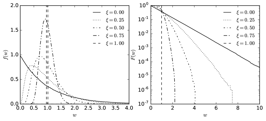
In Figure 2 we show the results of the simulation for $\xi=0.00$, $0.25$, $0.50$, $0.75$, $1.00$. The wealth distribution that results by mixing these these two antagonistic operators is similar to a Gamma distribution. Here we have considered a population of $N=1000$ agents with an initial wealth $W=N$, uniformly distributed among them. The number of simulation steps was set to $10^{6}$, and we averaged over $10^{4}$ initial configurations. The results for the Gini coefficient, $G(\xi)$, and the first mode, $\mu$, of the distribution are also shown Table 1.

	$\xi=0.00$	$\xi=0.25$	$\xi=0.50$	$\xi=0.75$	$\xi=1.00$
$G$	0.500	0.365	0.246	0.129	0.000
$\mu$	0.000	0.454	0.776	0.922	1.000

The Gini coefficient takes the maximum value $G=0.5$ for $\xi=0$, corresponding to the Boltzmann-Gibbs distribution, and gradually decreases to the minimum value $G=0$, corresponding to the Dirac distribution, as the parameter $\xi$ approaches $1$. The mode $\mu$ of the Gamma-like distribution increases with $\xi$, from $0$ (Boltzmann-Gibbs) to $1$ (Dirac delta).

The above operators can be generalized by considering that the money exchange between the agents is governed by two independent uniform random variables, $\varepsilon,\rho\sim U[0,1]$, such that the local conservation rule is still respected. Thus we have:

$$T^{+}(\varepsilon,\rho)=\begin{bmatrix}\varepsilon&\rho\\ 1-\varepsilon&1-\rho\end{bmatrix}$$ (20)

and respectively:

$$T^{-}(\varepsilon,\rho)=\begin{bmatrix}\varepsilon&1-\rho\\ 1-\varepsilon&\rho\end{bmatrix}$$ (21)

One can see that both operators are column stochastic matrices, and they are both invertible for $\varepsilon\neq\rho$, which suggests a different behaviour.

Figure 3: Probability distribution function $f(w)$, and cumulative distribution function $F(w)$, for the statistically equivalent operators $T^{+}(\varepsilon,\rho)\equiv T^{-}(\varepsilon,\rho)$.

The result of these operators is obviously different when they act locally on a pair of agents. However, their "global" statistical behaviour is the same if $\varepsilon$ and $\rho$ are independent uniform distributed random variables, sampled at every iteration step:

$$T^{+}(\varepsilon,\rho)\equiv T^{-}(\varepsilon,\rho)$$ (22)

which means that they are "statistically equivalent".

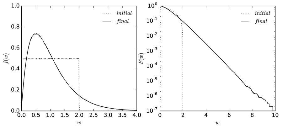
Our numerical simulations show that these operators transform any initial distribution into a Gamma distribution:

$$f(w)=\frac{w^{k-1}e^{-w/\theta}}{\Gamma(k)\theta^{k}}$$ (23)

with $k=2$, $\theta=2$, and a Gini coefficient:

$$G=\frac{\Gamma(5/2)}{2\Gamma(2)\sqrt{\pi}}=0.375$$ (24)

In Figure 3 we give such an example, where the initial distribution corresponds to a population of $N=1000$ agents with an initial wealth $W=N$, uniformly distributed among them. The number of simulation steps was set to $10^{6}$, and we averaged over $10^{4}$ initial configurations.

Let us now consider a heterogeneous model, where the agents have a different "personality", which is described by the following operator:

$$T^{+}(\varepsilon_{i},\rho_{j})=\begin{bmatrix}\varepsilon_{i}&\rho_{j}\\ 1-\varepsilon_{i}&1-\rho_{j}\end{bmatrix}$$ (25)

Here, the parameters $\varepsilon_{n},\rho_{n},n=1,...,N$ can be interpreted as the risk aversion of the agents, and they are initially drawn from a uniform random distribution $U[0,1]$, and contrary to the previous models they are kept frozen during the computation.

Figure 4: Pareto distribution with index $\nu\simeq 2$ for the operator $T^{+}(\varepsilon_{i},\rho_{j})$, with fixed values $\varepsilon_{i},\rho_{j}\sim U[0,1]$, $i,j=1,...,N$ (left); and the Pareto law with index $\nu\simeq 1$ for the heterogeneous savings model (right). The dashed red line is the fit with the Pareto distribution.

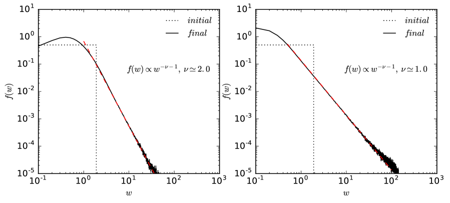
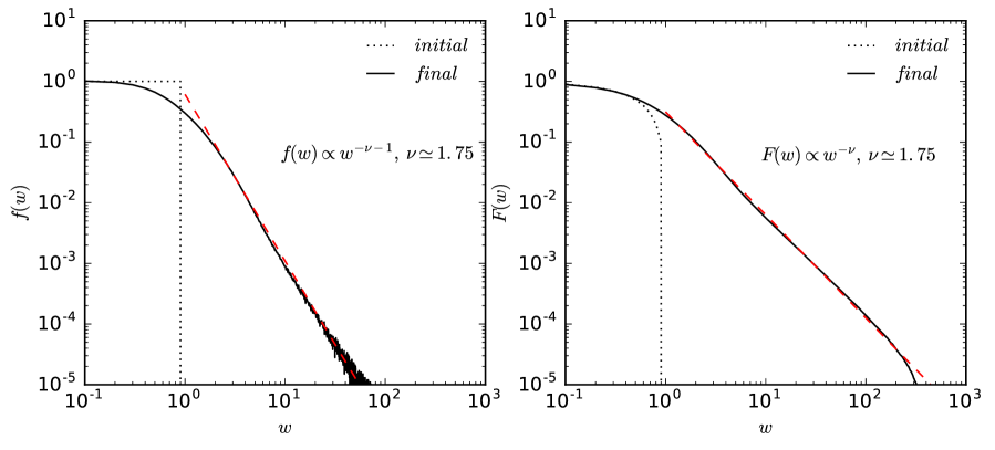
The obtained result is quite different, and it shows a unimodal distribution with a Pareto tail with the index $\nu\simeq 2$, Figure 4 (left). The Gini coefficient of the distribution in this example is $G=0.447$. The dashed red line in Figure 4 is the fit with the Pareto distribution.

For comparison we have also considered the heterogeneous savings model, which generates a Pareto distribution with an index $\nu\simeq 1$, and a much larger Gini coefficient $G=0.759$, Figure 4 (right) [14]. Thus the distribution generated by the operator $T^{+}(\varepsilon_{i},\rho_{j})$ is more "fair" than the distribution generated by the heterogeneous savings model, indicating more wealth accumulated by the middle class.

The explanation for this difference is that the parameters in the models are different. The heterogeneous savings model can be written as following [14]:

$$w^{\prime}_{i} =\lambda_{i}w_{i}+\eta[(1-\lambda_{i})w_{i}+(1-\lambda_{j})w_{j}]$$

$$w^{\prime}_{j} =\lambda_{j}w_{j}+(1-\eta)((1-\lambda_{i})w_{i}+(1-\lambda_{j})w_{j})$$ (26)

where $\lambda_{i}\sim U[0,1]$ are the fixed saving propensities of the agents, and $\eta\in U[0,1]$ is a uniform random variable. We notice that this model can be also rewritten in a matrix form as:

$$\begin{bmatrix}w^{\prime}_{i}\\ w^{\prime}_{j}\end{bmatrix}=T^{+}(\varepsilon^{\prime}_{i}(\eta,\lambda_{i}),\rho^{\prime}_{j}(\eta,\lambda_{j}))\begin{bmatrix}w_{i}\\ w_{j}\end{bmatrix}$$ (27)

with:

$$\varepsilon^{\prime}_{i}(\eta,\lambda_{i}) =1-(1-\eta)(1-\lambda_{i})$$

$$\rho^{\prime}_{j}(\eta,\lambda_{j}) =(1-\eta)(1-\lambda_{j})$$ (28)

Thus, the models have similar equations, and we could have expected to obtain similar results. However, the results are quite different due to the difference in the definition of their parameters.

Figure 5: Pareto distribution with index $\nu\simeq 1.75$ for the operator $T^{+}(\varepsilon_{i},\rho_{j})$, with fixed values $\varepsilon_{i},\rho_{j}\in(0,1)$, $i,j=1,...,N$ drawn from the square of a uniform random distributed variable. The dashed red line is the fit with the Pareto distribution.

The parameters $\varepsilon_{i}$, $\rho_{j}$ in the operator $T^{+}(\varepsilon_{i},\rho_{j})$ are initially drawn from a uniform random distribution $U[0,1]$, and then kept frozen during the simulation, while the parameters $\varepsilon^{\prime}_{i}$ and $\rho^{\prime}_{j}$ in the heterogeneous savings model correspond to the product of a uniform distributed random variable $x\equiv 1-\eta$, changing randomly at every step, and $y\equiv 1-\lambda_{j}$ which is also kept frozen.

The index of the Pareto law can be further modified by changing the distribution of the parameters $\varepsilon_{i}$ and $\rho_{j}$ in $T^{+}(\varepsilon_{i},\rho_{j})$. For example, if $\varepsilon_{i}$ and $\rho_{j}$ are drawn from $1-\xi^{2}$, where $\xi$ is a uniform random variable $\xi\sim U[0,1]$, then the index becomes $\nu\simeq 1.75$, as show in Figure 5. The Gini coefficient for the distribution in this example also increases to $G=0.596$.

The changes in the Pareto index can be explained by the fact that the density function of $1-\xi^{2}$ is not uniform any more. The density function of $1-\xi^{2}$ can be easily calculated by first calculating the cumulative distribution as follows:

$$F_{1-\xi^{2}}(\xi) =\text{Pr}(1-\xi^{2}\leq x)$$

$$=\text{Pr}(x\in[\sqrt{1-\xi},1])$$

$$=1-\sqrt{1-\xi}$$ (29)

Thus, the density function of $1-\xi^{2}$ is:

$$f_{1-\xi^{2}}(\xi)=\frac{dF_{1-\xi^{2}}(\xi)}{d\xi}=\frac{1}{2\sqrt{1-\xi}}$$ (30)

A smaller Pareto index $\nu\simeq 1.6$ is obtained if the parameters $\varepsilon_{i}$ and $\rho_{j}$ are drawn from $1-\xi^{4}$, where $\xi\sim U[0,1]$. This means that the Pareto index decreases by further increasing the probability of higher risk aversion parameters.

Therefore, the index of the Pareto distribution in these models strongly depends on the distribution of the parameters $\varepsilon_{i}$ and $\rho_{j}$ in the operator $T^{+}(\varepsilon_{i},\rho_{j})$.

4 Conclusion

We have discussed the role of a class of conservative local operators, that can be used to reproduce the main features of empirical distributions observed in the previous kinetic models of wealth distribution: Boltzmann-Gibbs, Dirac delta, Gamma and Pareto. Numerical simulations have shown that in order to generate the power-law tail an heterogeneous risk aversion model is required. In this case, the Pareto index strongly depends on the distribution of the risk aversion parameters. Also, we have shown numerically that by changing the parameters of these operators one can also fine tune the resulting distributions in order to provide support for the emergence of a more egalitarian wealth distribution.

As a closing remark, we would like to note that these results can be further extended to more complex agent models in econophysics and sociophysics, where a binary exchange mechanism between the agents is expected (market models, opinion formation etc.). Also, this class of local conservative operators can be applied to more relaxed cases where the local exchanged quantities are only conserved in the mean:

$$w^{\prime}_{i}+w^{\prime}_{j}=\langle w_{i}+w_{j}\rangle,$$ (31)

removing the strong pointwise conservation constraint, and allowing for a more complex stochastic dynamics where other mechanisms like debt and interest can be taken into account.

References

- [1] V. Pareto, Cours d’economie Politique (F. Rouge, Lausanne, 1897).
- [2] Gibrat, R., Les Inégalités Economiques Sirely (Paris, 1931).
- [3] S. Moss de Oliveira, P.M.C. de Oliveira and D. Stauffer, Evolution, Money, War and Computers (B.G. Tuebner, Stuttgart, Leipzig, 1999).
- [4] M. Levy, S. Solomon, Physica A 242, 90 (1997).
- [5] H. Aoyama, W. Souma, Y. Fujiwara, Physica A 324, 352 (2003)
- [6] F. Clementi, M. Gallegati, Physica A 350, 427 (2005)
- [7] A. Banerjee, V.M. Yakovenko, T.Di Matteo, Physica A 370, 54 (2006).
- [8] S. Sinha, Physica A 359, 555, (2006).
- [9] A.A. Dragulescu, V.M. Yakovenko, Eur. Phys. J. B 20, 585 (2001)
- [10] A.A. Dragulescu, V.M. Yakovenko, Physica A 299, 213 (2001)
- [11] V.M. Yakovenko, J. Barkley Rosser Jr., Rev. Mod. Phys. 81, 1703 (2009)
- [12] A.A. Dragulescu, V.M. Yakovenko, Eur. Phys. J. B 17, 723 (2000)
- [13] A. Chakraborti, B.K. Chakrabarti, Eur. Phys. J. B 17, 167 (2000).
- [14] A. Chatterjee, B.K. Chakrabarti, S.S. Manna, Physica A 335, 155 (2004).
- [15] S. Guala, Int. Desc. Comp. Sys. 7, 1 (2009)
- [16] C. Gini, Rivista di Politica Economica 87, 769 (1997).
- [17] P.M. Dixon, J. Weiner, T. Mitchell-Olds, R. Woodley, Ecology 68, 1548 (1987).
- [18] C. Damgaard, J. Weiner, Ecology 81, 1139 (2000).
- [19] A.K. Gupta, Physica A 359, 634 (2006).