Abstract: A number of studies, referring to the observed Trojan asteroids of various planets in our Solar System, or to hypothetical Trojan bodies in extrasolar planetary systems, have emphasized the importance of so-called secondary resonances in the problem of the long term stability of Trojan motions. Such resonances describe commensurabilities between the fast, synodic, and secular frequency of the Trojan body, and, possibly, additional slow frequencies produced by more than one perturbing bodies. The presence of secondary resonances sculpts the dynamical structure of the phase space. Hence, identifying their location is a relevant task for theoretical studies. In the present paper we combine the methods introduced in two recent papers ([21], [22]) in order to analytically predict the location of secondary resonances in the Trojan problem. In [21], the motion of a Trojan body was studied in the context of the planar Elliptic Restricted Three Body (ERTBP) or the planar Restricted Multi-Planet Problem (RMPP). It was shown that the Hamiltonian admits a generic decomposition $H=H_{b}+H_{sec}$. The term $H_{b}$, called the basic Hamiltonian, is a model of two degrees of freedom characterizing the short-period and synodic motions of a Trojan body. Also, it yields a constant ‘proper eccentricity’ allowing to define a third secular frequency connected to the body’s perihelion precession. $H_{sec}$ contains all remaining secular perturbations due to the primary or to additional perturbing bodies. Here, we first investigate up to what extent the decomposition $H=H_{b}+H_{sec}$ provides a meaningful model. To this end, we produce numerical examples of surfaces of section under $H_{b}$ and compare with those of the full model. We also discuss how secular perturbations alter the dynamics under $H_{b}$. Secondly, we explore the normal form approach introduced in [22] in order to find an ‘averaged over the fast angle’ model derived from $H_{b}$, circumventing the problem of the series’ limited convergence due to the collision singularity at the 1:1 MMR. Finally, using this averaged model, we compute semi-analytically the position of the most important secondary resonances and compare the results with those found by numerical stability maps in specific examples. We find a very good agreement between semi-analytical and numerical results in a domain whose border coincides with the transition to large-scale chaotic Trojan motions.

1 Introduction

Ever since the discovery of the triangular equilibrium solutions of the Three Body Problem by Lagrange (1772), the problem of the dynamical behavior of the orbits near the equilateral equilibrium points has attracted great interest in the astronomical community. A long known application refers to the family of Trojan asteroids of Jupiter (see [25] and references therein). Trojan asteroids were found also around other planets in our solar system, i.e. the Earth, Mars, Uranus and Neptune ([4], [5], [1]). On different grounds, a number of works have adressed the questions of the overall existence, formation and detectability of Trojan exoplanets ([3], [6]). No such body has been identified so far in exoplanet surveys. This may indicate that such planets are rare, which case would necessitate a dynamical explanation, or that there exist yet unsurpassed constrains in exo-Trojan detectability. It has been proposed that the complexity of the orbits of Trojan bodies may itself introduce intricacies in possible methods of detection, see, for example, [15] refering to the Transit Timing Variation method; regarding, in particular, the radial velocity measurements, see [7]. The above and other examples emphasize the need to understand in detail the orbital dynamics in the 1:1 Mean Motion commensurability.

In the present paper we extend the work of two previous papers ([22], [21]), in the direction of developing an efficient analytical method for the study of Trojan orbital dynamics. The aim of analytical studies is to identify the main features of the phase space and to quantify their role in the dynamical behavior of the orbits. Some important references of past analytical studies of the Trojan problem can be found in [12] and references therein.

Regarding past approaches, the following is a key remark. Most analytical treatments of the Trojan problem in the literature are so far based upon series expansions of the equations of motion around the stable equilibria $L_{4}$ and $L_{5}$, using various sets of variables (e.g cartesian, cylindrical, or Delaunay-like action-angle variables). However, it is important to recall that all these kinds of expansions exhibit an important limitation, related to the singular behavior of the equations of motion at relatively large Trojan libration amplitudes. In the framework of the ERTBP, defined by a central mass, a perturber body and a massless particle (the Trojan body), this singular behavior corresponds geometrically to an approach of the Trojan body close to the perturbing body, which is possible only at the 1:1 Mean Motion Resonance. The relevant remark is that, the presence of a singularity in the equations of motion implies a finite disc of convergence for any kind of series expansions around $L_{4}$ or $L_{5}$. It is straightforward to see that the projection of this disc in configuration space is such so as to render the series’ convergence very poor for orbits with large libration amplitudes not only towards the perturber, but also in the direction opposite to the perturber, i.e. towards the unstable colinear point $L_{3}$. Let us note that this poor convergence has a pure mathematical origin; no physical singularity actually exists exactly at or close to $L_{3}$.

The following is a more precise form of the above remark. Let $\theta$ be the angular distance between the perturber and the Trojan body, e.g. in a heliocentric frame. Regardless the initial choice of variables, model approximation, etc., one finally recovers for $\theta$ a differential equation of the form (see, for example, [10])

$${d^{2}\theta\over dt^{2}}+3\mu\sin\theta\left[1-2^{-3/2}(1-\cos\theta)^{-3/2}\right]+\mbox{h.o.t.}=0\leavevmode\nobreak\ \leavevmode\nobreak\$$ (1)

where $\mu$ is the mass parameter of the perturber. The higher order terms include epyciclic oscillations, the eccentricity of the Trojan or the perturber, as well as any other kind of perturbation induced, for example, by more perturbing bodies. Ignoring such terms, Eq. (1) can be thought of as Newton’s equation corresponding to a ‘potential’

$$V(\theta)=3\mu\left[{1\over\sqrt{2-2\cos\theta}}-\cos\theta\right]\leavevmode\nobreak\ \leavevmode\nobreak\ .$$ (2)

This differs only by a constant from the quantity $H(\theta)$ introduced in [19], called also the ‘ponderomotive potential’ in [20]. If, instead, one expresses the equations of motion in orbital elements, one encounters equivalent terms in the disturbing function ([19] §6), taking the form $\mu[-\cos\tau+(1-\cos\tau)^{-1/2}]$, where $\tau=\lambda-\lambda^{\prime}$ corresponds to the critical argument of the 1:1 Mean Motion commensurability, $\lambda$, $\lambda^{\prime}$ being the mean longitudes of the Trojan and the perturber respectively. The position of $L_{4}$ (or $L_{5}$) corresponds to $\theta_{0}=\tau_{0}=\pi/3$ (or $5\pi/3$). Setting $u=\theta-\theta_{0}$ or $u=\tau-\tau_{0}$ and expanding the equations of motion in powers of the quantity $u$ leads to expressions converging in the domain $|u|<\pi/3$. The convergence is quite slow for angles approaching the limiting values $u_{lim}\pm\pi/3$. In reality, such expansions become unpractical for libration angles $\sim 30^{\circ}$ and beyond, i.e. after half way to the singularity. The applicability of all analytical methods based on polynomial expansions around $L_{4}$ or $L_{5}$ is severely limited by this poor convergence.

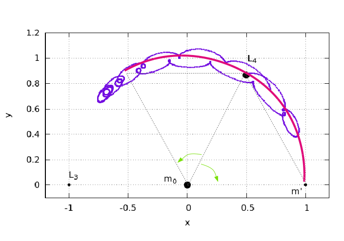
Figure 1: Representation of the domain of $\tau$ where polynomial series are convergent if the expansion takes place around $L_{4}$, in a heliocentric cartesian frame co-rotating with the perturber $(x,y)$. The position of the equilibrium points $L_{4}$ and $L_{3}$, the central mass $m_{0}$ and the perturber $m^{\prime}$ are indicated with black points. The radius of convergence (thick pink line) of the series is given by the distance between $L_{4}$ and the perturber, namely $60^{\circ}$ ($\tau=\pi/3$). While this does not induce any problem in the direction towards the perturber, it does limit the convergence in the opposite direction. In purple, we show an example of a typical Trojan orbit, obtained by numerically integrating the equations of motion of the ERTBP, for the initial condition $(x,y,\dot{x},\dot{y})=(0.507,0.87402,0,0)$. The orbit clearly exceeds the leftward limit of $60^{\circ}$ from $L_{4}$.

On the other hand, one finds numerically that stable tadpole orbits exist in domains extending well beyond the limits of convergence of the analytical methods (see Fig. 1).

In [22], a new method of series expansions for the Trojan problem was introduced, aiming, precisely, to remedy the poor convergence of the classical series expansions around $L_{4}$ or $L_{5}$. The method was developed in the context of the canonical formalism. In more detail, an algorithm was derived allowing to compute a so-called Hamiltonian normal form for Trojan motions. In the normal form approach, starting from an initial Hamiltonian model, one performs a series of near-identity canonical transformations from old to new canonical variables, leading to a new expression for the Hamiltonian (called the ‘normal form’). Via these transformations, the goal is to arrive at a new form of the equations of motion in the new variables, which is simpler to solve than in the original variables. In [22] the algorithm was applied to the simplest possible model, namely the planar and circular Restricted Three Body Problem (CRTBP). In this case, the normal form becomes an integrable model of one degree of freedom, allowing to analytically approximate the motion in the so-called synodic (associated with the libration motion around $L_{4}$) degree of freedom. The key point of the method is that the functional dependence of all involved quantities (i.e. normal form, transformation equations etc., see section 3 below for details) on the quantity

$$\beta_{0}={1\over\sqrt{1-\cos\tau}}$$ (3)

and on the powers of $\beta_{0}$ is maintained at all orders of perturbation theory. Hence, the so-resulting series are not affected by the singularity at $\tau=0$ (i.e. $u=-\pi/3$) and remain useful practically within the whole tadpole domain.

In the present paper we implement the method developed in [22] in a model more realistic than the CRTBP, namely the model introduced in [21]. This provides an approximation to the Trojan dynamics applicable to two distinct cases: i) the planar Elliptic Restricted Three Body Problem (ERTBP), and ii) what was called in [21] the ‘Restricted Multi-Planet Problem’ (RMPP). In the latter case, we assume that there are more than one perturbing bodies which exert secular perturbations on the Trojan body. The main application in mind is a hypothetical Trojan exoplanet in a multi-planet extrasolar system, although the model applies equally well to the Trojan asteroids of giant planets in our solar system. The RMPP exhibits a more rich spectrum of secular perturbations than the ERTBP. Even so, in [21] it was shown that in both problems, one can derive a so-called, ‘basic Hamiltonian model’ (denoted hereafter as $H_{b}$). The Hamiltonian $H_{b}$ approximates the dynamics in the fast and synodic degrees of freedom. Furthermore, in [21] it was shown that $H_{b}$ is formally identical in the ERTBP and the RMPP (apart from a re-interpretation of the physical meaning of one pair of action-angle variables). Consequently, the two problems are formally diversified only by their different sets of secular terms in the Hamiltonian, denoted by $H_{sec}$. Let us note that here, as in [21], we focus only on the planar version of the $H_{b}$ model, although generalization to the spatial version is straightforward.

Combining the results of [21] and [22], we provide below an application of particular interest, namely, the semi-analytical determination of the location of secondary resonances in the tadpole domain of motion. As was shown in [13], secondary resonances play a key role in determining the boundary and the size of the tadpole stability domain.

In [21] a combination of numerical indicators (the Fast Lyapunov Indicator - FLI [14], as well as the NAFF (Numerical Analysis of the Fundamental Frequencies) algorithm [16] were used to identify the most important secondary resonances in a space corresponding to what is known as the ‘proper elements’ of the Trojan body’s motion (see [17], [2], as well as the definitions in [21]). As an example, in the case of the ERTBP, the location of various secondary resonances was determined in the space of proper elements, depending mainly on two parameters, i.e., the perturber’s mass parameter $\mu$ and eccentricity $e^{\prime}$. In the present paper, we demonstrate, instead, the efficiency of the analytical normal form approach of [22] in identifying the location of secondary resonances in the space of proper elements.

The structure of the paper is as follows: in Section 2 we examine some features of the ‘basic Hamiltonian’ model of [21], and validate the usefulness of the decomposition $H=H_{b}+H_{sec}$ by performing a numerical exploration of the dynamics under $H_{b}$ alone, as well as of how the latter compares to the full Hamiltonian dynamics. Then, in Section 3 we implement the normal form method introduced in [22] to the Hamiltonian $H_{b}$, and check its performance in the location of the secondary resonances. Section 4 summarizes our conclusions.

2 Basic Hamiltonian $H_{b}$: construction and features

In this section, we aim to explore in some detail the features of the Hamiltonian model introduced in [21], and to discuss the advantages and the limitations in the approximations of this model. For completeness, we begin by briefly reviewing the construction of the model. For more details, we defer the reader to [21].

2.1 Construction

In the framework of the planar elliptic Restricted Three Body Problem (pERTBP), the equations of motion of the Trojan body (’massless body’) depend on two physical parameters: i) the mass parameter $\mu=\frac{m^{\prime}}{m^{\prime}+M}$, where $M$ is the mass of the central mass and $m^{\prime}$ the mass of the perturber (also ’primary perturber’ or simply ’primary’), and ii) the eccentricity of the heliocentric orbit of the primary perturber, $e^{\prime}$. In the ERTBP $e^{\prime}$ and the major semi-axis of the primary’s orbit are constant, set $a^{\prime}=1$ in our units.

In [21], a Hamiltonian formulation was provided for the Trojan motion, in the pERTBP, and also in a more complex problem where $S$ additional perturbing bodies (e.g. planets) are present, being mutually far from MMRs. The Hamiltonian of the ’Restricted Multi-Planet Problem’ (RMPP) was written in [21] under the form

$$H =H_{b}\,(Y_{f},\phi_{f},u,v,Y_{p};\mu,e^{\prime}_{0})$$ (4)

$$+\,H_{sec}\,(Y_{f},\phi_{f},u,v,Y_{p},\phi,P^{\prime},I_{1},\ldots I_{S},\phi^{\prime},\phi_{1},\ldots,\phi_{S})\leavevmode\nobreak\ \leavevmode\nobreak\ .$$

In Eq. (4), the variables $(\phi_{f},Y_{f})$, $(u,v)$ and $(\phi,Y_{p})$ are pairs of action-angle variables, whose definition stems from Delaunay-like variables following a sequence of four consecutive canonical transformations (see Appendix). The reader is deferred to Section 2 of [21] for the details, while a schematic description of the physical meaning of these variables is given in Fig. 2. On the other hand, the angle $\phi^{\prime}=g^{\prime}t$ corresponds to the longitude of the pericenter of the primary perturber (constant in the pERTBP, precessing in the RMPP), while the angles $\phi_{j}=g_{j}t$ account for the secular perturbations induced by the $S$ additional perturbers. These angles are canonically conjugate to a set of (dummy) action variables denoted by $P^{\prime}$ and $I_{j}$ respectively. Finally, $e_{0}^{\prime}$ is the average eccentricity of the primary perturber, which coincides with $e^{\prime}$ in the pERTBP.

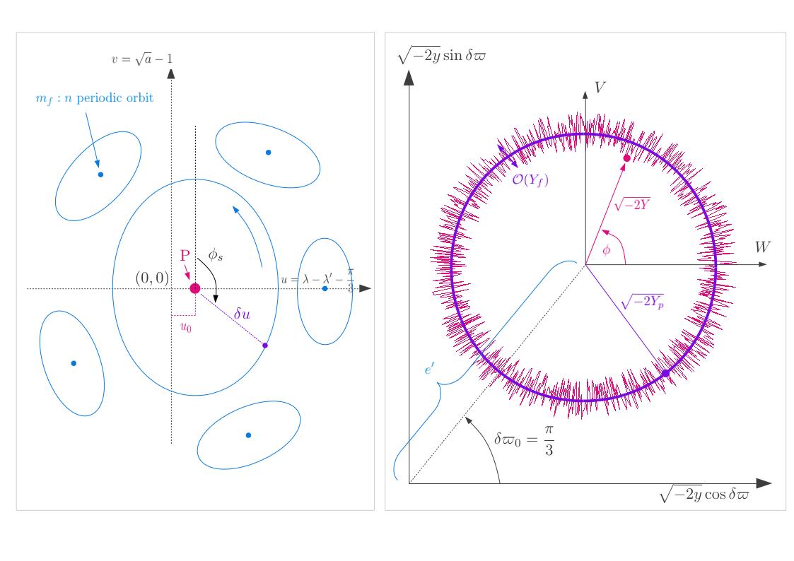
Figure 2: Schematic representation of the physical meaning of the action-angle variables used for the Hamiltonian $H_{b}$ in (5). The plane $(u,v)$ corresponds to the ‘synodic’ motion of the Trojan body, where $u=\lambda-\lambda^{\prime}-\pi/3$ ($\lambda$ and $\lambda^{\prime}$ correspond to the mean longitude of the Trojan body and the primary, respectively) and $v=\sqrt{a}-1$ ($a$ is the major semi-axis of the Trojan and $a^{\prime}=1$ for the primary). Under the Hamiltonian $H_{b}$, the phase portrait can be represented by a Poincaré surface of section corresponding, e.g., to every time when the angle $\phi_{f}$ accomplishes a full cycle. The left panel shows the form of the projection of this section on the plane $(u,v)$. The central point P represents a stable fixed point corresponding to the short-period periodic orbit around $L_{4}$. The orbit has frequency $\omega_{f}$, while its amplitude increases monotonically with $Y_{f}$. The forced equilibrium corresponds to $u_{0}=0$, $Y_{f}=0$. The point P, however, has in general a shift to positive values $u_{0}>0$ for proper eccentricities $e_{p}$ larger than zero. On the surface of section, the frequency of libration around the periodic orbit is given by the synodic frequency $\omega_{s}$. Resonances, and their island chains, correspond to rational relations between the fast frequency $\omega_{f}$ and $\omega_{s}$. On the other hand, the plane $(W,V)=(\sqrt{-2y}\cos\delta\varpi,\sqrt{-2y}\sin\delta\varpi,)$ with $y=\sqrt{a}(\sqrt{1-e^{2}}-1)$ and $\delta\varpi=\varpi-\varpi^{\prime}$ the difference of longitude of perihelion of the Trojan and the primary (right panel) depicts the evolution of the Trojan body’s eccentricity vector under the Hamiltonian $H_{b}$. The motion of the endpoint of the eccentricity vector can be decomposed to a circulation around the forced equilibrium, with angular frequency $g$, and a fast (of frequency $\omega_{f}$) ‘in-and-out’ oscillation with respect to a circle of radius $e_{p}$, of amplitude which is of order ${\cal O}(Y_{f})$. All extra terms with respect to $H_{b}$ in the Hamiltonian (4) depend on the slow angles $(\phi,\phi^{\prime})$ in pERTBP, and also on the angles $\phi_{j}$, $j=1,\ldots,S$ in the RMPP. Thus, all these terms can only slowly modulate the dynamics under $H_{b}$.

We call the term $H_{b}$ in the Hamiltonian of Eq. (4) the ‘basic Hamiltonian model’ for Trojan motions in the 1:1 MMR. Its detailed form is given in the Supplementary Online Material of [21]. We find

$$H_{b}=-\frac{1}{2(1+v)^{2}}-v+(1+g^{\prime})Y_{f}-g^{\prime}Y_{p}-\mu{\cal F}^{(0)}(u,\phi_{f},v,Y_{f}-Y_{p};e_{0}^{\prime})\leavevmode\nobreak\ \leavevmode\nobreak\ .$$ (5)

The function ${\cal F}^{(0)}$, contains terms depending on the canonical pairs $(\phi_{f},Y_{f})$ and $(u,v)$. The former characterizes fast motions (with frequency $\omega_{f}\sim{\cal O}(1)$), while the latter characterizes the ‘long-period’ synodic motions (with frequency $\omega_{s}\sim{\cal O}(\sqrt{\mu})$). On the other hand, since the angle $\phi$ (see Fig. 2) is ignorable in $H_{b}$, the action variable $Y_{p}$ is an integral of the basic Hamiltonian. This allows to define also a secular frequency via $g=\dot{\phi}=\partial H_{b}/\partial Y_{p}$. More precisely, we recover the well known relations (e.g., [11])

$$\omega_{f}\equiv\dot{\phi}_{f}=1-\frac{27}{8}\,\mu+g^{\prime}+\ldots\leavevmode\nobreak\ \leavevmode\nobreak\ ,$$ (6)

$$\omega_{s}\equiv\dot{\phi}_{s}=-\sqrt{\frac{27\mu}{4}}+\ldots\leavevmode\nobreak\ \leavevmode\nobreak\ ,$$ (7)

$$g\equiv\dot{\phi}=\frac{27}{8}\,\mu-g^{\prime}+\ldots\leavevmode\nobreak\ \leavevmode\nobreak\ .$$ (8)

On the other hand, the higher order corrections in Eqs. (6), (7), (8), can be recovered by an efficient normal form approach, as shown in Section 3 below.

Three additional remarks concerning $H_{b}$ are:

i) The constancy of $Y_{p}$ under $H_{b}$ allows to define an approximation to the quasi-integral of the proper eccentricity $e_{p}$ (see [21]) via

$$e_{p}=\sqrt{-2Y_{p}}\leavevmode\nobreak\ \leavevmode\nobreak\ .$$ (9)

This approximation remains useful in the whole spectrum of models ranging from the CRTBP to the full RMPP.

ii) In Eq. (5), the dependence of ${\cal F}^{(0)}$ on the actions $Y_{p}$ and $Y_{f}$ is exclusively via the difference $Y_{f}-Y_{p}$. This fact allows to simplify some normal form computations, as shown in Subsection 2.2 below. We can define, in respect, an eccentricity parameter

$$e_{p,0}=\sqrt{-2Y}=\sqrt{2Y_{f}-2Y_{p}}\leavevmode\nobreak\ \leavevmode\nobreak\ .$$ (10)

The quantity $e_{p,0}$ will be used below in labeling several solutions found via the study of $H_{b}$.

iii) By construction, $H_{b}$ is formally identical in the RMPP and in the pERTBP, with the substitution $e^{\prime}_{0}\rightarrow e^{\prime}$ and setting $g^{\prime}=0$. Thus, the determination of the frequencies $\omega_{f}$, $\omega_{s}$ and $g$ based on a normal form manipulation of $H_{b}$ as below (Section 3) leads to equivalent results regardless the number of additional perturbing bodies besides the primary.

On the other hand, $H_{sec}$ in (4) gathers all the terms of $H$ depending on the slow (secular) angle $\phi$ (with frequency $g\sim{\cal O}(\mu)$), or, in the case of the RMPP, also on the slow angles $\phi^{\prime}$, $\phi_{j}$, $j=1,\ldots S$ (of frequencies ${\cal O}(\mu_{j})$). As a consequence, in [21] it was proposed that the dynamics at secondary resonances can be approximated as a slow modulation of all the resonances produced by the basic model $H_{b}$, due to the additional influence of $H_{sec}$. Considering the RMPP with $S$ bodies, the most general form of a planar secondary resonance is given by

$$m_{f}\omega_{f}+m_{s}\omega_{s}+mg+m^{\prime}g^{\prime}+m_{1}g_{1}+\ldots+m_{s}g_{s}=0\leavevmode\nobreak\ \leavevmode\nobreak\ ,$$ (11)

where $m_{f}$, $m_{s}$, $m$, $m^{\prime}$, $m_{j}$ (with $j=1,\ldots,S$) are integers. Keeping the notation of [21], the most important secondary resonances are those present in the basic Hamiltonian model $H_{b}$, already if $e^{\prime}=0$, i.e. the resonances of the circular RTBP. These are denoted as the $m_{f}$:$m_{s}$ resonances, with comensurability relation

$$m_{f}\omega_{f}+m_{s}\omega_{s}=0\leavevmode\nobreak\ \leavevmode\nobreak\ .$$ (12)

The particular case when $m_{f}=1$ corresponds to the lowest order resonances that can be found for a certain value of the mass parameter $\mu$, and usually dominate the structure of the phase-space. These are called the ’main secondary resonances’ $1$:$n$, where $n=m_{s}$. For values of $\mu$ between $0.01$ and $0.0005$, $n$ corresponds to $4,5,6\ldots,16$. On the other hand, we collectively refer to any other resonance of the ERTBP (involving all 3 frequencies $\omega_{f}$, $\omega_{s}$ and $g$) as well as to more general cases of the RMPP (including the frequencies $g^{\prime}$, $g_{j}$) as ’transverse’ resonances.

2.2 Limits of applicability of the basic model $H_{b}$

The basic model $H_{b}$ represents a reduction of the number of degrees of freedom with respect to the original problem. Thus, we expect that its usefulness in approximating the full problem (ERTBP or RMPP) holds to some extent only. The following numerical examples aim to compare the dynamical behavior of the orbits under the $H_{b}$ and the full Hamiltonian. To this end, we compute and compare various phase portraits (surfaces of section) arising under the two Hamiltonians. We restrict ourselves to the comparison between $H_{b}$ and the full Hamiltonian of the ERTBP only. We thus set $e_{0}^{\prime}=e^{\prime}$, and $g^{\prime}=0$, $S=0$. Then, all secular perturbations are accounted for by only one additional degree of freedom with respect to $H_{b}$, represented by the canonical pair $(\phi,Y_{p})$. Integrating numerically the RMPP instead of the ERTBP is considerably more expensive. Still, it is arguable that the effect of the secular perturbations should remain qualitatively similar by adding more degrees of freedom consisting of slow action-angle pairs only, as in the Hamiltonian decomposition of Eq. (4).

Our numerical integrations of the full Hamiltonian model (ERTBP) are performed in heliocentric Cartesian variables, in which the equations of motion are straightforward to express. Whenever needed, translation from Cartesian to the canonical variables appearing in (4) and vice versa is done following the sequence of canonical transformations defined in [21].

On the other hand, for the basic Hamiltonian $H_{b}$ we have an explicit expression only in the latter variables. However, one can readily see that, for fixed $(u,v,\phi_{f})$, all the initial conditions of fixed difference $Y_{f}-Y_{p}$ lead to the same orbit, independently of the individual values of $Y_{f}$ or $Y_{p}$. If we set $Y_{f}=Y_{f,ref}=0$ and $Y_{p}=Y_{p,ref}=-e_{p,ref}^{2}/2$ for one particular orbit chosen in advance, that we call the ‘reference orbit’, this allows to specify a certain appropriate value of the energy $E=E_{ref}$ equal to the numerical value of $H_{b}$ for that orbit. The reference orbit satisfies the condition $e_{p,ref}=e_{p,0}$, i.e., $e_{p,0}$ becomes equal to the modulus of the initial vector $\mathbf{e}-\mathbf{e}_{forced}$, where $\mathbf{e}=(e\cos\omega,e\sin\omega)$, and $\mathbf{e}_{forced}=(e^{\prime}/2,e^{\prime}\sqrt{3}/2)$. Now, keeping both $Y_{p}=Y_{p,ref}$ and $E=E_{ref}$ fixed, but altering $(u,v,\phi_{f})$, allows to solve the equation $E_{ref}=H_{b}$ for $Y_{f}$ and specify new initial conditions for more orbits at the same energy as the reference orbit. However, now we will find in general that the initial value of $Y_{f}$ for any of these new orbits satisfies $Y_{f}\neq 0$. In terms of the initial eccentricity vector, this implies that $e_{p,0}\neq e_{p,ref}$. The so found orbit is the same as the one in which we set $Y_{p}=-e_{p,0}^{2}/2\neq Y_{p,ref}$, and $Y_{f}=0$. For convenience, we formally proceed with the former process (keeping $E=E_{ref}$ and $Y_{p}=Y_{p,ref}$ fixed and adjusting $Y_{f}$ for different initial conditions). However, since the value of the proper eccentricity for each of these initial conditions $e_{p,0}$, we label all plots by $e_{p,0}$ instead of $e_{p}$ in the FLI stability maps presented below as well as in [21].

Returning to our numerical computations, in order to choose a reference orbit we select one close to the short period family around $L_{4}$ [23]. More precisely, we set $u=v=\phi_{f}=Y_{f}=0$ for the reference orbit, and consider different values for $Y_{p}=Y_{p,ref}$. Physically, this means to choose different energy levels $E=E_{ref}$ at which the reference orbit has different proper eccentricity. Let us note that the existence of a central periodic orbit is itself a property of the basic model $H_{b}$; adding more degrees of freedom implies, instead, the existence of an invariant torus of dimension larger than one and smaller than the full number of degrees of freedom.

Having selected $E_{ref}$ and $Y_{p,ref}$, we compute initial conditions for more orbits at the energy $E=E_{ref}$. More precisely, in each of the figures which follow, we define a set of $19$ initial conditions given by $u_{j}=0.05\times j$, $v_{j}=0$, $\phi_{f,j}=0$, for $j=0,\ldots,18$, and $Y_{f,j}$ computed as described above. With these initial conditions, we numerically integrate the orbits, under the equations of motion of $H_{b}$, up to collecting, for each orbit, 500 points on the surface of section $\phi_{f}=0\,(\mathrm{mod}\>2\pi)$.

The same set of initial conditions is integrated under the equations of motion of the full ERTBP, for a time equivalent to 500 revolutions of the primary, collecting about 490 points in the same surface of section. In the ERTBP, the surface of section is four-dimensional, but a two-dimensional projection on the plane $(u,v)$ allows comparisons with the corresponding section of the basic model $H_{b}$.

As an additional comparison, we also compute the surface of section provided by an intermediate model between the $H_{b}$ and the pERTBP. We construct a 3 d.o.f Hamiltonian in the following way

$$H_{b,sec}=H_{b}\,(Y_{f},\phi_{f},u,v,Y_{p};\mu,e^{\prime},e_{p,0})+\langle F^{(1)}\rangle(u,v,Y_{p},\phi;\mu,e^{\prime},e_{p,0},Y_{f})\leavevmode\nobreak\ \leavevmode\nobreak\ ,$$ (13)

where

$$\langle F^{(1)}\rangle={1\over 2\pi}\int_{0}^{2\pi}H_{sec}d\phi_{f}\leavevmode\nobreak\ \leavevmode\nobreak\ .$$ (14)

Explicit formulae for $\langle F^{(1)}\rangle$ can be found in the Supplementary Online Material of [21]. Such terms may depend on the slow angle $\phi$, but are independent of the fast angle $\phi_{f}$. Hence, $H_{b,sec}$ contains some, but not all, the secular terms of the disturbing function of the pERTBP. On the other hand, up to first order in the mass parameter $\mu$, the averaging (14) yields the same Hamiltonian as the one produced by a canonical transformation eliminating all terms depending on the fast angle $\phi_{f}$. Thus, the model $H_{b,sec}$ captures the main effect of the secular terms, as discussed in [21], which is a pulsation, with frequency $g$, of the separatrices of all the secondary resonances induced by $H_{b}$. Since the modulation due to these secular terms is slow, far from secondary resonances we expect that an adiabatic invariant holds for initial conditions close to the invariant tori of $H_{b}$, thus yielding stable regular orbits. On the other hand, in [21] it was argued that close to secondary resonances the pulsation provokes a weak chaotic diffusion best described by the paradigm of modulational diffusion.

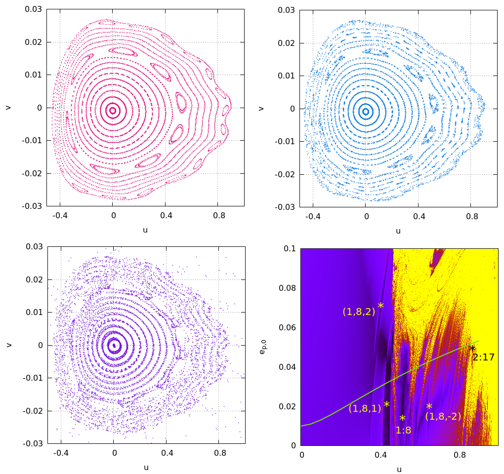
Figure 3: Comparison of surfaces of section (section condition $\phi_{f}=0$) provided by different models. The considered parameters are $\mu=0.0024$, $e^{\prime}=0.04$ and $e_{p,ref}=0.01$. In pink points (upper left), we show the surface of section provided by $H_{b}$. In blue points (upper right), the one corresponding to $H_{b,sec}$. In purple points (lower left), the one corresponding to pERTBP. In lower right panel, we reproduce the FLI map of [21] corresponding to the physical parameters $\mu$ and $e^{\prime}$ considered, with the most important secondary resonances indicated. The color-scale for the FLI map goes as follows: dark colors (purple) indicate regular orbits, while light colors (yellow) indicate for the chaotic orbits (see [21] for the exact FLI computation). The green line on the FLI map indicates the isoenergetic curve where the initial conditions are located.

Figure 4: Same as in Fig. 3, but for a higher parameter value $e_{p,ref}=0.035$.

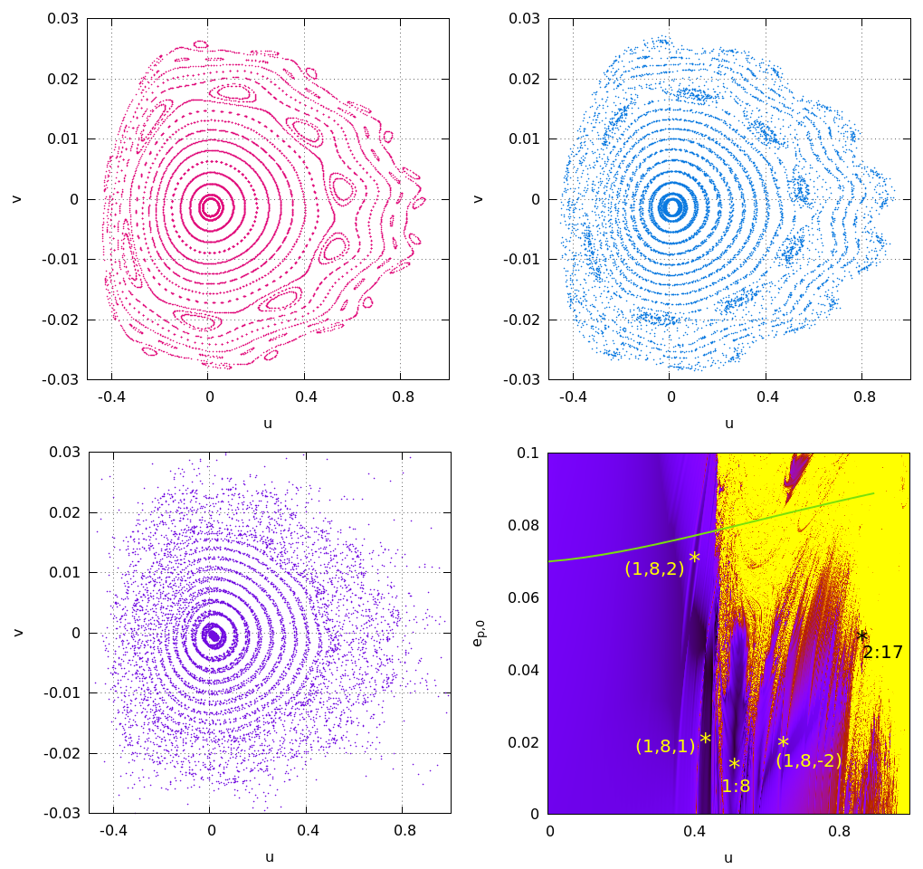
Figure 5: Same as in Fig. 3, but for a still higher parameter value $e_{p,ref}=0.07$.

Figures 3, 4 and 5 show an example of the comparison between the three mentioned above models. The physical parameters chosen for these plots are $\mu=0.0024$ (which depicts clearly the 1:8 main secondary resonance) and $e^{\prime}=0.04$. Figure 3 shows the surface of section $\phi_{f}=0\,(\mathrm{mod}\>2\pi)$ corresponding to $e_{p,ref}=0.01$, Fig. 4 to $e_{p,ref}=0.035$ and Fig. 5 to $e_{p,ref}=0.07$. In each figure, the upper left plot (pink points) corresponds to the surface of section produced by the flow under the basic model $H_{b}$, the upper right plot (blue points) to the flow under $H_{b,sec}$ and the lower left plot (purple points) to the flow under the full Hamiltonian of the pERTBP. As an additional information, we provide the FLI stability map corresponding to the same parameters $\mu$ and $e^{\prime}$, which was computed in Fig. 8c of [21] (see that paper for details on the FLI computation). On top of the FLI map, in green we show the locus of initial conditions $(u,e_{p,0})$ on the surface of section whose orbits have constant energy $E=E_{ref}$.

In Fig. 3, in the approximation based on the model $H_{b}$, the absence of any dependence of the dynamics on the slow angle $\phi$ renders possible to clearly display the short period and synodic dynamics by means of the surface of section $\phi_{f}=0\,(\mathrm{mod}\>2\pi)$, which, for $H_{b}$, is two-dimensional. In fact, for more complex models like $H_{b,sec}$ or the full pERTBP, the corresponding surface of section is 4-dimensional and its 2D projection on the $(u,v)$ plane becomes blurred (top right and bottom left panels respectively). The blurring can be due partly to projection effects. However, we argue below that an important effect is caused also by the influence of the secular terms, absent in $H_{b}$, to the dynamics.

Returning to the phase portrait of $H_{b}$, this allows to extract relevant information such as: i) the position of the central fixed point, corresponding to the crossing of the section by the short period orbit, ii) several secondary resonances and the corresponding resonant islands of stability, and iii) the overall size of the libration domain of effective stability. Also, this phase portrait allows to understand the structure of the stability map. In the phase portrait, as we move from left to right along the line $x=0$, we encounter non-resonant tori, interrupted by thin chaotic layers and the islands of some secondary resonances, namely the resonances 1:8 (at $u\sim 0.55$) and 2:17 (at $u\sim 0.85$). Note, however, that no transverse secondary resonances can be seen in the $H_{b}$ portrait, since these resonances correspond, in general, to a non-resonant frequency ratio of the fast and synodic frequencies $\omega_{f}$ and $\omega_{s}$; except at resonance junctions, the exact resonance condition $m_{f}\omega_{f}+m_{s}\omega_{s}+m_{g}g=0$ for some non-zero $m_{s}$, $m_{f}$, $m_{g}$ implies, in general, non-commensurable values of $\omega_{f}$ and $\omega_{s}$. Since $q\ll\omega_{s}\ll\omega_{f}$, most transverse resonances can only accumulate close to the main secondary resonances forming resonant multiplets, as confirmed by visual inspection of the stability maps (see also [21]). However, some isolated transverse resonances may be embedded in the main domain of stability whose border is marked by the most conspicuous secondary resonance. In Fig. 3, this domain extends up to about $u\approx 0.5$. In the stability map of Fig. 3, the transverse resonances $[1,-8,k]$, with $k=-2,-1,1,2$ form a multiplet together with the conspicuous resonance $1$:$8$. Two of these transverse resonances ($k=2$ and $k=1$) are embedded in the main domain of stability. However, none of the transverse resonances is visible in the phase portrait of the basic model $H_{b}$.

We now discuss the pulsation effect of the phase portrait due to the slow modulation induced by the secular terms. As shown in [21], the amplitude of the secular terms depends on the values of $e^{\prime}$ and $e_{p,0}$. For fixed $e^{\prime}\neq 0$, the amplitude of the pulsation generated by such terms increases with $e_{p,0}$. For values of $e_{p,0}$ large enough, the pulsation modifies the whole behavior in phase-space. Since, along the line $x=0$, $e_{p,0}$ increases with $u$ (green curve in low-right panel of Fig. 3), the amplitude of the pulsation increases as we move from the central fixed point outwards. In regions where the resonant web is dense enough, this pulsation causes all narrow transverse resonances in a multiplet to overlap, increasing the size of the chaotic domain and facilitating escaping mechanisms. For the set of parameters of Fig. 3, we see from the corresponding FLI map that this happens for values of $e_{p,0}$ greater than about $0.06$. Beyond this value, the effect induced by $H_{sec}$ implies that the blurring observed in the phase portraits (apart from the one of $H_{b}$) is not due just to projection effects but it has a dynamical origin, the nature of the orbits changes as they are converted from regular to chaotic. Evidence of this phenomenon is found, e.g, in the case of the resonance 2:17. While in the surface of section of the $H_{b}$, the 2:17 stability islands are clearly seen, such resonance is not evident in the surfaces of section of the ERTBP and $H_{b,sec}$. As represented by the FLI map, the effect of the resonance’s separatrix pulsation results in that no libration domain is identifiable in the FLI map.

This latter effect is more conspicuous in Figs. 4 and 5, in which, choosing a higher $e_{p,ref}$, we increase the level of proper eccentricities of all the orbits. In Fig. 4, the FLI stability map shows large domains of chaos which are not observed in the phase portrait of $H_{b}$, but they appear in the phase portrait of the full model. The separatrix pulsation of the 1:8 resonance is not, however, large enough so as to completely wash out this resonance, which is therefore seen in all four panels of the plot. On the other hand, increasing still more the level of proper eccentricities (Fig. 5) makes this pulsation large enough so as to completely introduce chaos in the position of the 1:8 resonance. This limit of eccentricity levels marks the overall validity of the approximation based on $H_{b}$ regarding the position of secondary resonances. Beyond this value, $H_{b}$ still represents fairly well the dynamics only inside the main librational domain of stability. We note also that the elimination of the main secondary resonance 1:8 by the separatrix pulsation is already present in the model $H_{b,sec}$ (compare the corresponding phase portraits in the three Figures 3, 4, 5).

In conclusion, the pulsation mechanism induced by the secular terms in the Hamiltonian affects essentially the regions of the phase space where resonances accumulate in the form of multiplets. For libration orbits, these are the regions beyond the main secondary resonance $1$:$n$, which always dominates the phase-space. The regions inner to that resonance are not influenced considerably and the representation of the dynamics via the basic model $H_{b}$ remains accurate there, even for high values of the proper eccentricity. The value of the latter at which the separatrix pulsation of the $1$:$n$ resonance completely washes this resonance marks the overall limit of approximation of the basic model. On the other hand, most orbits beyond that limit turn to be chaotic and fast-escaping the libration domain, thus of lesser interest in applications related to Trojan or exo-Trojan objects.

3 Normal form

In [22], a new normalizing scheme was introduced for the Hamiltonian of the planar Circular Restricted Three Body Problem (pCRTBP). Here, we adapt the scheme in order to compute a normal form in the case of the basic model $H_{b}$ derived from the pERTBP. The particular application considered is the semi-analytic determination of the position of the secondary resonances in the plane of the Trojan body’s proper elements.

3.1 Hamiltonian preparation

The novelty of the normalizing scheme introduced in [22] lies on the way the scheme deals with the synodic degree of freedom, expressed in the Hamiltonian through the variables $(u,v)$. For obtaining the dynamics in the synodic variables via a normal form, it is only necessary to average the Hamiltonian $H_{b}$ over the fast angle $\phi_{f}$. The novelty consists of retaining the original non-polynomial and non-trigonometric-polynomial functional dependence of the Hamiltonian on the synodic angle $u$ in all normal form expansions. As pointed out in the introduction, this allows to deal efficiently with the model’s singular behavior at $u=-\pi/3$.

We start by first expressing the basic model $H_{b}$ in variables appropriate for introducing the normalization scheme of [22]. The synodic degree of freedom is represented by the variables

$$v=x-x_{0},\quad u=\tau-\tau_{0}\leavevmode\nobreak\ \leavevmode\nobreak\ ,$$ (15)

where

$$x=\sqrt{a}-1\,,\quad\,\tau=\lambda-\lambda^{\prime}\leavevmode\nobreak\ \leavevmode\nobreak\ ,$$ (16)

$a$ being the major semi-axis of the Trojan body, and $\lambda$, $\lambda^{\prime}$ the mean longitudes of the Trojan body and the primary respectively. The constants $x_{0}$ and $\tau_{0}$ in (15) give the position of the forced equilibrium of the Hamiltonian averaged over $\lambda^{\prime}$ (see [21]). In the case of the pERTBP, in the vicinity of $L_{4}$, we have $x_{0}=0$, $\tau_{0}=\pi/3$. Finally, it turns convenient to introduce new canonical pairs: $(\phi_{f},\leavevmode\nobreak\ {\cal Y}=Y_{f}-Y_{p})$, and $(\theta=\phi+\phi_{f},\leavevmode\nobreak\ Y_{p})$. After these preliminary transformations, the basic model $H_{b}$ reads

$$H_{b}=-\frac{1}{2(1+x)^{2}}-x+{\cal Y}+Y_{p}-\mu{\cal F}^{(0)}(\tau,\phi_{f},x,{\cal Y};e^{\prime})\leavevmode\nobreak\ \leavevmode\nobreak\ .$$ (17)

The dependence of $H_{b}$ on $\tau$ is of the form $\frac{\cos^{k_{1}}\tau}{(2-2\cos\tau)^{j/2}}$ or $\frac{\cos^{k_{2}}\tau}{(2-2\cos\tau)^{j/2}}$, $j=2n-1$ with $k_{1}$, $k_{2}$ and $n$ integers (see Supplementary Online Material of [21]). Also, since the angle $\theta$ is ignorable, $Y_{p}$ is a constant that can be viewed as a parameter in $H_{b}$.

In order to initialize the normalization procedure, we write and expand the Hamiltonian in (17), by introducing modified Delaunay-Poincaré variables, as in [22]

$$x \,,\qquad\tau\,$$ (18)

$$\xi =\sqrt{2{\cal Y}}\cos\phi_{f}\,,$$

$$\eta =\sqrt{2{\cal Y}}\sin\phi_{f}\,\leavevmode\nobreak\ \leavevmode\nobreak\ .$$

The new expression for the Hamiltonian reads

$$H_{b}(\tau,x,\xi,\eta,Y_{p})=-\frac{1}{2(1+x)^{2}}-x+Y_{p}+\frac{\xi^{2}+\eta^{2}}{2}-\mu{\cal F}^{(0)}(\tau,x,\xi,\eta;Y_{p},e^{\prime})\leavevmode\nobreak\ \leavevmode\nobreak\ .$$ (19)

Finally, we expand the Hamiltonian in terms of every variable except $\tau$, obtaining

$$H_{b}(\tau,x,\xi,\eta,Y_{p})= -x+\sum_{i=0}^{\infty}\,(-1)^{i-1}(i+1)\,\frac{x^{i}}{2}\,+\,\frac{\xi^{2}+\eta^{2}}{2}\,+\,Y_{p}$$ (20)

$$+ \,\mu\sum_{\begin{subarray}{c}m_{1},m_{2},m_{3}\\ k_{1},k_{2},k_{3},j\end{subarray}}a_{m_{1},m_{2},m_{3},k_{1},k_{2},j}\,e^{\prime k_{3}}x^{m_{1}}\,\xi^{m_{2}}\,\eta^{m_{3}}\,\cos^{k_{1}}(\tau)\,\sin^{k_{2}}(\tau)\,\beta^{j}(\tau)\leavevmode\nobreak\ \leavevmode\nobreak\ ,$$

where $a_{m_{1},m_{2},m_{3},k_{1},k_{2},j}$ is a rational number and $\beta(\tau)=\frac{1}{\sqrt{2-2\cos\tau}}$. The Hamiltonian $H_{b}$ in (20) represents the ‘normal form at the zero-th step in the normalizing scheme’, i.e., before any normalization. This we denote as $H^{(1,0)}$.

4 Normalizing scheme

The normalizing algorithm defines a sequence of Hamiltonians by an iterative procedure. In order to simplify some of the concepts below we define the class ${\cal P}_{s,l}$ as the set of functions whose expansion is of the form

$$\sum_{2m_{1}+m_{2}+m_{3}=l}\,\,\sum_{\begin{subarray}{c}k_{1}+k_{2}\leq l+4s-3\\ j\leq 2l+7s-6\end{subarray}}a_{m_{1},m_{2},m_{3},k_{1},k_{2},j}\,e^{\prime k_{3}}x^{m_{1}}\,\xi^{m_{2}}\,\eta^{m_{3}}\,\cos^{k_{1}}(\tau)\,\sin^{k_{2}}(\tau)\,\beta^{j}(\tau)\leavevmode\nobreak\ \leavevmode\nobreak\ .$$ (21)

Let $r_{1},\,r_{2}$ be two integer counters, $1\leq r_{1}\leq R_{1}$ and $1\leq r_{2}\leq R_{2}$ with fixed $R_{1},R_{2}\in\mathbb{N}$. We assume that at a generic normalizing step ($r_{1}$,$r_{2}-1$), the expansion of the Hamiltonian is given by

$$H^{(r_{1},r_{2}-1)}(x,\xi,\tau,\eta,Y_{p})= \,Y_{p}+\frac{\xi^{2}+\eta^{2}}{2}+\sum_{i=2}^{\infty}\alpha_{i}\,x^{i}$$ (22)

$$+ \,\sum_{s=1}^{r_{1}-1}\sum_{l=0}^{R_{2}}\mu^{s}Z_{s,l}\,(x,(\xi^{2}+\eta^{2})/2,\tau)$$

$$+ \,\sum_{l=0}^{r_{2}-1}\mu^{r_{1}}Z_{r_{1},l}\,(x,(\xi^{2}+\eta^{2})/2,\tau)$$

$$+ \,{\cal R}^{(r_{1},r_{2}-1)}(x,\xi,\eta,\tau)\leavevmode\nobreak\ ,$$

where $\alpha_{i}$ are real coefficients and the remainder ${\cal R}^{(r_{1},r_{2}-1)}(x,\xi,\eta,\tau)$ is given by

$${\cal R}^{(r_{1},r_{2}-1)} \,(x,\xi,\eta,\tau)=\mu^{r_{1}}f_{r_{1},r_{2}}^{(r_{1},r_{2}-1)}(x,\xi,\eta,\tau)+\sum_{l=r_{2}+1}^{R_{2}}\mu^{r_{1}}f_{r_{1},l}^{(r_{1},r_{2}-1)}(x,\xi,\eta,\tau)$$ (23)

$$+ \,\sum_{s=r_{1}+1}^{\infty}\sum_{l=0}^{R_{2}}\mu^{s}f_{s,l}^{(r_{1},r_{2}-1)}(x,\xi,\eta,\tau)+\sum_{s=1}^{\infty}\sum_{r=R_{2}+1}^{\infty}\mu^{s}f_{s,l}^{(r_{1},r_{2}-1)}(x,\xi,\eta,\tau)\leavevmode\nobreak\ .$$

All the terms $Z_{s,l}$ and $f_{s,l}^{(r_{1},r_{2}-1)}$ appearing in (22) are made by expansions including a finite number of monomials of the type given by the class ${\cal P}_{s,l}$. More specifically $Z_{s,l}\in{\cal P}_{s,l}$ $\forall\ 0\leq l\leq R_{2}\,,\ 1\leq s<r_{1}\,$, $Z_{r_{1},l}\in{\cal P}_{r_{1},l}$ $\forall\ 0\leq l<r_{2}\,$, $f_{r_{1},l}^{(r_{1},r_{2}-1)}\in{\cal P}_{r_{1},l}$ $\forall\ l\geq r_{2}\,$, $f_{s,l}^{(r_{1},r_{2}-1)}\in{\cal P}_{s,l}$ $\forall\ l>R_{2}\,,\ 1\leq s<r_{1}\,$ and $\forall\ l\geq 0,\ s>r_{1}\,$.

In formula (22), one can distinguish the terms in normal form from the remainder ${\cal R}$: the latter depend on $(\xi,\eta)$ in a generic way, while in the normal form terms $Z$, those variables just appear under the form $(\xi^{2}+\eta^{2})/2$. The $(r_{1},r_{2})$–th step of the algorithm formally defines the new Hamiltonian $H^{(r_{1},r_{2})}$ by applying the Lie series operator $\exp{\cal L}_{\mu^{r_{1}}\chi_{r_{1},r_{2}}}$ to the previous Hamiltonian $H^{(r_{1},r_{2}-1)}$, as it follows

$$H^{(r_{1},r_{2})}=\exp\left({\cal L}_{\mu^{r_{1}}\chi_{r_{1},r_{2}}}\right)H^{(r_{1},r_{2}-1)}\leavevmode\nobreak\ \leavevmode\nobreak\ .$$ (24)

The Lie series operator is given by

$$\exp\left({\cal L}_{\chi}\right)\,\cdot\,=\sum_{j\geq 0}\frac{1}{j!}{\cal L}_{\chi}^{j}\;\cdot\leavevmode\nobreak\ \leavevmode\nobreak\ ,$$ (25)

where the Lie derivative ${\cal L}_{\chi}g=\{g,\chi\}$, is such that $\{\cdot,\cdot\}$ is the classical Poisson bracket. The new generating function $\mu^{r_{1}}\chi_{r_{1},r_{2}}$ is determined by solving the following homological equation with respect to the unknown $\chi_{r_{1},r_{2}}=\chi_{r_{1},r_{2}}(x,\xi,\tau,\eta)$:

$${\cal L}_{\mu^{r_{1}}\chi_{r_{1},r_{2}}}Z_{0,2}+f_{r_{1},r_{2}}^{(r_{1},r_{2}-1)}=Z_{r_{1},r_{2}}\leavevmode\nobreak\ \leavevmode\nobreak\ ,$$ (26)

where $Z_{0,2}=\frac{\xi^{2}+\eta^{2}}{2}$ and $Z_{r_{1},r_{2}}$ is the new term in the normal form, i.e. $Z_{r_{1},r_{2}}=Z_{r_{1},r_{2}}(x,\tau,(\xi^{2}+\eta^{2})/2)$. In other words, $\mu^{r_{1}}\chi_{r_{1},r_{2}}$ is determined so as to remove the terms that do not belong to the normal form from the main perturbing term $\mu^{r_{1}}f_{r_{1},r_{2}}^{(r_{1},r_{2}-1)}$. Thus, by construction, the new Hamiltonian $H^{(r_{1},r_{2})}$ inherits the structure of Eq. (22). From the latter, we point out that the splitting of the Hamiltonian in sub-functions of the form ${\cal P}_{s,l}$, organizes the terms in groups with the same order of magnitude $\mu^{s}$ and total degree $l/2$ (possibly semi-odd) in the variables $x$ and ${\cal Y}=\frac{\xi^{2}+\eta^{2}}{2}$. This way, we exploit the existence of the natural small parameters of the model in the normalizing procedure. Furthermore, after having omitted the constant term $\alpha_{0}\,$, we can set the Hamiltonian $H_{b}$ in (20) as the first normalizing step Hamiltonian $H^{(1,0)}$, according to (22).

The algorithm requires just $R_{1}\cdot R_{2}$ normalization steps, constructing the finite sequence of Hamiltonians

$$H^{(1,0)}=H_{b},\,H^{(1,1)},\,\ldots,\,H^{(1,R_{2})},\,H^{(2,1)},\,\ldots,\,H^{(R_{1},R_{2})}\leavevmode\nobreak\ \leavevmode\nobreak\ .$$ (27)

Here, we add the prescription that $H^{(r_{1},0)}=H^{(r_{1}-1,R_{2})}\,\forall\,1<r_{1}\leq R_{1}$. Then, we write the final Hamiltonian, where we distinguish the normal form part from the remainder, as

$$H^{(R_{1},R_{2})}(x,\xi,\tau,\eta,Y_{p})={\cal Z}^{(R_{1},R_{2})}\left(x,\frac{(\xi^{2}+\eta^{2})}{2},\tau,Y_{p}\right)+{\cal R}^{(R_{1},R_{2})}(x,\xi,\tau,\eta)\leavevmode\nobreak\ \leavevmode\nobreak\ .$$ (28)

At this point, we must remark a few features of the normal form ${\cal Z}^{(R_{1},R_{2})}$. While its dependence on $x$ and $\tau$ remains generic, it depends on $\xi$ and $\eta$ only through the form $\frac{\xi^{2}+\eta^{2}}{2}$. That is, we have

$$H^{(R_{1},R_{2})}(x,\tau,{\cal Y},\phi_{f},Y_{p})={\cal Z}^{(R_{1},R_{2})}\left(x,\tau,{\cal Y},Y_{p}\right)+{\cal R}^{(R_{1},R_{2})}(x,\tau,{\cal Y},\phi_{f})\leavevmode\nobreak\ \leavevmode\nobreak\ .$$ (29)

The key remark is that $\phi_{f}$ becomes ignorable in the normal form, and, therefore, ${\cal Y}$ becomes an integral of motion of ${\cal Z}^{(R_{1},R_{2})}$. Then, the normal form can be viewed as a Hamiltonian of one degree of freedom depending on two constant actions ${\cal Y}$ and $Y_{p}$, i.e. ${\cal Z}^{(R_{1},R_{2})}$ represents now a formally integrable dynamical system. Of course, since the true system is not integrable, it is natural to expect that the normalization procedure diverges in the limit of $R_{1},R_{2}\rightarrow\infty$. The divergence corresponds formally to the fact that the size of the remainder function ${\cal R}^{(R_{1},R_{2})}$ cannot be reduced to zero as the normalization order tends to infinity. Then, the optimal normal form approximation corresponds to choosing the values of both integer parameters $R_{1}$ and $R_{2}$ so as to reduce the size of the remainder ${\cal R}^{(R_{1},R_{2})}$ as much as possible. In practice, there are computational limits that compromise the choice of values of $R_{1}$ and $R_{2}$. In all subsequent computations, the values are $R_{1}=2$ and $R_{2}=4$, corresponding to a second order expansion and truncation on the mass parameter $\mu$ and fourth order for the total polinomial degree of $x$, $\xi$ and $\eta$. These normalization orders prove to be sufficient for the normal form to represent a good representation of the original Hamiltonian in the domain of regular motions. In particular, we will now employ this possibility in order to compute the positions of different secondary resonances, based on the integrable approximation provided by our normal form.

4.1 Application: determination of the location of resonances via the normal form

Consider an orbit with initial conditions specified in terms of the two parameters $u=\tau-\tau_{0}$ and $e_{p,0}$ in the same way as in the stability maps of Figures 3, 4, 5. We will make use of the normal form approximation $Z^{(R_{1},R_{2})}$ in (29) in order to compute the values of the three main frequencies of motion for the given initial conditions. The computation proceeds by the following steps:

1) We first evaluate the synodic frequency $\omega_{s}$, i.e., the frequency of libration of the synodic variables $\tau$ and $x$. The normal form $Z^{(R_{1},R_{2})}$ leads to Hamilton’s equations:

$$\frac{\textrm{d}x}{\textrm{d}t}=f(x,\tau;{\cal Y})=-\frac{\partial Z^{(R_{1},R_{2})}}{\partial\tau}\leavevmode\nobreak\ \leavevmode\nobreak\$$ (30)

and

$$\frac{\textrm{d}\tau}{\textrm{d}t}=g(x,\tau;{\cal Y})=-\frac{\partial Z^{(R_{1},R_{2})}}{\partial x}\leavevmode\nobreak\ \leavevmode\nobreak\ .$$ (31)

For every orbit we can define the constant energy

$$Z^{(R_{1},R_{2})}(x,\tau;{\cal Y},Y_{p})-Y_{p}\equiv\zeta^{(R_{1},R_{2})}(x,\tau;{\cal Y})={\cal E}\leavevmode\nobreak\ \leavevmode\nobreak\ .$$ (32)

Note that since $Y_{p}$ appears only as an additive constant in $Z^{(R_{1},R_{2})}$, the function $\zeta^{(R_{1},R_{2})}$ does not depend on $Y_{p}$. Also, according to (10) and (18), we have ${\cal Y}=\frac{e_{p,0}^{2}}{2}$. Then, for fixed value of ${\cal E}$, we can express $\tau$ as an explicit function of $x$,

$$\zeta^{(R_{1},R_{2})}(x,\tau;{\cal Y})={\cal E}\quad\Longrightarrow\quad\tau=\tau({\cal E},x;{\cal Y})\leavevmode\nobreak\ \leavevmode\nobreak\ .$$ (33)

Replacing (33) in (30), we get

$$\frac{\textrm{d}x}{\textrm{d}t}=f(x,\tau({\cal E},x;{\cal Y});{\cal Y})\quad\Longrightarrow\quad\text{d}t=\frac{\text{d}x}{f(x,\tau({\cal E},x;{\cal Y});{\cal Y})}\leavevmode\nobreak\ \leavevmode\nobreak\ ,$$ (34)

whereby we can derive an expression for the synodic period $T_{syn}$

$$T_{syn}=\oint\frac{\text{d}x}{f(x,\tau({\cal E},x;{\cal Y});{\cal Y})}\leavevmode\nobreak\ \leavevmode\nobreak\ ,$$ (35)

and thus the synodic frequency

$$\omega_{s}=\frac{2\pi}{T_{syn}}\leavevmode\nobreak\ \leavevmode\nobreak\ .$$ (36)

In practice, (33) is hard to invert analytically, and hence, the integral (35) cannot be explicitly computed. We thus compute both expressions numerically on grids of points of the associated invariant curves on the plane $(\tau,x)$, or by integrating numerically (34) as a first order differential equation.

2) We now compute the fast and secular frequencies $\omega_{f}$, $g$. To compute $\omega_{f}$, we use the equation

$$\omega_{f}=\,\frac{1}{T_{syn}}\int_{0}^{T_{syn}}\frac{\textrm{d}\phi_{f}}{\textrm{d}t}\,\textrm{d}t=\,\frac{1}{T_{syn}}\int_{0}^{T_{syn}}\frac{\partial Z^{(R_{1},R_{2})}(x,\tau;{\cal Y})}{\partial{\cal Y}}\,\textrm{d}t\leavevmode\nobreak\ \leavevmode\nobreak\ .$$ (37)

Replacing (34) in (37), we generate an explicit formula for the fast frequency

$$\omega_{f}=\frac{1}{T_{syn}}\oint\frac{1}{f(x,\tau({\cal E},x;{\cal Y});{\cal Y})}\,\frac{\partial Z_{R_{1},R_{2}}(x,\tau({\cal E},x;{\cal Y});{\cal Y})}{\partial{\cal Y}}\,\textrm{d}x\leavevmode\nobreak\ \leavevmode\nobreak\ .$$ (38)

Since $Z^{(R_{1},R_{2})}(x,\tau;{\cal Y},Y_{p})=Y_{p}+\zeta^{(R_{1},R_{2})}(x,\tau;{\cal Y})$ we find $\dot{\theta}=1$ implying $g=1-\omega_{f}$.

All the frequencies are thus functions of the labels ${\cal E}$ and ${\cal Y}$, which, in the integrable normal form approximation, label the proper libration and the proper eccentricity of the orbits. In the normal form approach one has $e_{p,0}=e_{p}=$ const, implying ${\cal Y}=e_{p}^{2}/2$. If, as in [21], we fix a scanning line of initial conditions $x_{in}=Bu_{in}=\tau_{in}-\tau_{0}$, with $B$ a constant, the energy ${\cal E}$, for fixed $e_{p}$, becomes a function of the initial condition $u_{in}$ only. Thus, $u_{in}$ represents an alternative label of the proper libration (see Section 3 of [21] for a detailed discussion of this point). With these conventions, all three frequencies become functions of the labels $(u_{in},e_{p})$. A generic resonance condition then reads

$$\Phi_{m_{f},m_{s},m}(u)=m_{f}\omega_{f}(e_{p},u_{in})+m_{s}\omega_{s}(e_{p},u_{in})+mg(e_{p},u_{in})=0\leavevmode\nobreak\ \leavevmode\nobreak\ .$$ (39)

For fixed resonance vector $(m_{f},m_{s},m)$, Eq. (39) can be solved by root-finding, thus specifying the position of the resonance on the plane of the proper elements $(u_{in},e_{p})$.

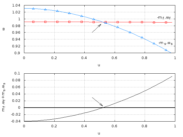
Figure 6: Representation of the evolution of the frequencies as function of $u$. In the upper panel, $m_{f}\omega_{f}$ (red square points) and $-m_{s}\omega_{s}$ (blue triangle points). In the lower panel, the evolution of the function $m_{f}\omega_{f}+m_{s}\omega_{s}$ (black curve). The arrows denote the point where the frequencies accomplish the resonant condition $m_{f}\omega_{f}+m_{s}\omega_{s}=0$, giving the position of the resonance in terms of $u$. For this example, we choose the resonance $1$:$8$, corresponding to $m_{f}=1$, $m_{s}=8$, $\mu=0.0024$, $e^{\prime}=0.04$ and a representative value for $e_{p,0}=0.05$.

As an example, Fig. 6, shows $\omega_{f}$ and $\omega_{s}$, as well as the function $\Phi_{1,8,0}(e_{p},u_{in})$, as a function of $u_{in}$ for the parameters $\mu=0.0024$, $e^{\prime}=0.04$ and a fixed value of $e_{p}=0.05$. The arrow in the lower panel marks the position of the resonance. Changing the value of $e_{p}$ in the same range as the one considered in our numerical FLI stability maps ($0<e_{p,0}<0.1$), we specify $u_{in}$ all along the locus of the resonance projected in the stability map. Repeating this computation for several transverse resonances $(m_{f},m_{s},m)$, we are able to trace the location of each of them.

In order to test the accuracy of the above method, we compare the results of the semi-analytical estimation with the position of the resonances extracted from the FLI maps computed in [21]. Under the assumption that the local minimum of the FLI in the vicinity of a resonance gives a good approximation of the resonance center, we study the curves of the FLI $\Psi$ as a function of $u$, for a fixed value of $e_{p,0}$. Figure 7 gives an example for $\mu=0.0031$, $e^{\prime}=0.04$, $e_{p,0}=0.015$, where we choose four candidates as centers of the resonances $(1,7,1)$, $1$:$7$, $(1,7,-1)$ and $(1,7,-2)$. We confirm the resonant character of these orbits also by performing a numerical Frequency Analysis [16]. By changing the value of $e_{p,0}$ along the interval $[0,0.1]$, we can depict the centers of the resonances on top of the FLI maps.

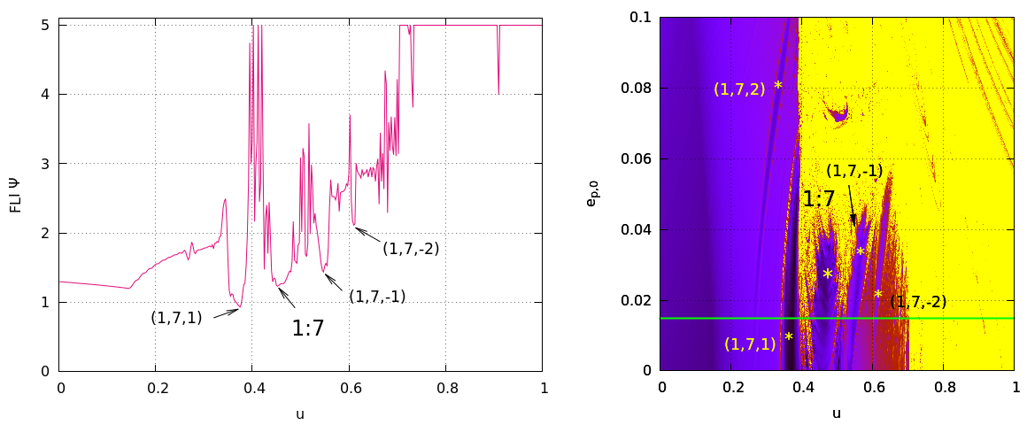
Figure 7: FLI $\Psi$ as function of $u$, for fixed parameters $\mu\leavevmode\nobreak\ =\leavevmode\nobreak\ 0.0031$, $e^{\prime}\leavevmode\nobreak\ =\leavevmode\nobreak\ 0.04$ and $e_{p,0}\leavevmode\nobreak\ =\leavevmode\nobreak\ 0.015$ (right panel). The local minima give a good approximation of the position of the centers of each resonance. The orbits whose corresponding FLI values are plotted in the left panel lie on the green line on top of the FLI map (right panel). The confirmation of each resonance is done by frequency analysis.

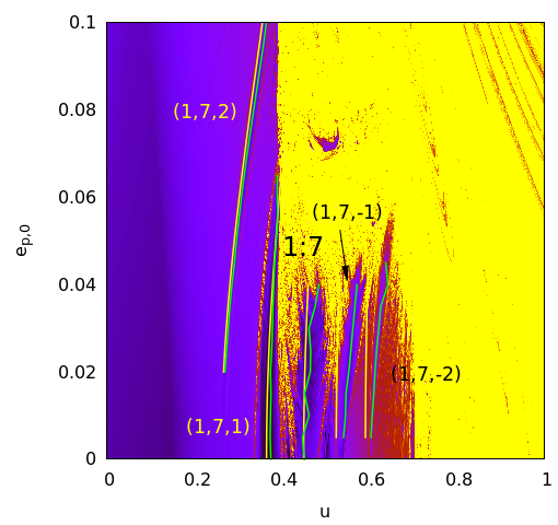
Figure 8: Main and transverse secondary resonances located by $Z^{(R_{1},R_{2})}$ (yellow) and the estimation of FLI $\Psi$ minima (green). In this example, $\mu=0.0031$, $e^{\prime}=0.04$, $m_{f}=1$, $m_{s}=7$, $m=0,\pm 1,\pm 2$. Labels indicate the corresponding resonance in each case.

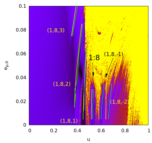
Figure 9: Same as Fig. 8, for $\mu=0.0024$, $e^{\prime}=0.06$, and $m_{f}=1$, $m_{s}=8$, $m=0,\pm 1,\pm 2,3$.

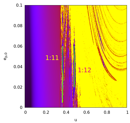
Figure 10: Same as Fig. 8, for $\mu=0.0014$, $e^{\prime}=0.02$, and $m_{f}=1$, $m_{s}=11,12$, $m=0$.

Resonance	$\mu$, $e^{\prime}$	$\overline{u_{{\cal Z}}}$	$\overline{u_{\Psi}}$	$\overline{\delta u_{in}}$
$1$:$7$	$0.0031$, $0.04$	0.453908	0.463308	2.129422${\scriptstyle\times 10}^{[}-2]$
$(1,7,1)$	′′	0.377456	0.380947	1.417910${\scriptstyle\times 10}^{[}-2]$
$(1,7,2)$	′′	0.306036	0.312011	1.880279${\scriptstyle\times 10}^{[}-2]$
$(1,7,-1)$	′′	0.527218	0.554430	4.885329${\scriptstyle\times 10}^{[}-2]$
$(1,7,-2)$	′′	0.593373	0.618057	3.964370${\scriptstyle\times 10}^{[}-2]$
$1$:$8$	$0.0024$, $0.06$	0.524485	0.535153	1.993063${\scriptstyle\times 10}^{[}-2]$
$(1,8,1)$	′′	70.465475	0.464924	6.377401${\scriptstyle\times 10}^{[}-3]$
$(1,8,2)$	′′	0.406439	0.412246	1.605145${\scriptstyle\times 10}^{[}-2]$
$(1,8,3)$	′′	0.374879	0.385020	2.617987${\scriptstyle\times 10}^{[}-2]$
$(1,8,-1)$	′′	0.587834	0.616093	4.572688${\scriptstyle\times 10}^{[}-2]$
$(1,8,-2)$	′′	0.646464	0.679154	4.796435${\scriptstyle\times 10}^{[}-2]$
$1$:$11$	$0.0014$, $0.02$	0.367663	0.370842	9.264243${\scriptstyle\times 10}^{[}-3]$
$1$:$12$	′′	0.482117	0.486631	1.021940${\scriptstyle\times 10}^{[}-2]$

Table 1: Averaged values of $u_{{\cal Z}}$, $u_{{\Psi}}$ and $\delta u_{in}$ for the resonances in Figures 8, 9 and 10

Figures 8, 9 and 10 show examples of these computations, for the parameters $\mu=0.0031$ and $e^{\prime}=0.04$, $\mu=0.0024$ and $e^{\prime}=0.06$, $\mu=0.0014$ and $e^{\prime}=0.02$, respectively. The normal form predictions are superposed as yellow lines upon the underlying FLI stability maps while the centers of each resonance, as extracted from the FLI maps, are denoted by the green curves. Due to the numerical noise in the FLI curves, it is not possible to clearly extract the position of the resonance centers for all values of $e_{p,0}$, while a semi-analytic estimation (with varying levels of accuracy) is always possible. At any rate, in Figs. 8-10, we compare the position of the resonaces only in these cases when both methods provide clear results. Table 1 summarizes the results for the location of the centers ($u_{{\cal Z}}$, $u_{\Psi}$) and the relative errors ($\delta u_{in}=\frac{|u_{{\cal Z}}-u_{\Psi}|}{u_{\Psi}}$), on average, for the resonances shown in the corresponding figures.

Regarding the overall performance of the estimation, we can note that the level of approximation is very good for relatively low values of $\mu$, $e_{p}$ and $u_{in}$, while the error in the predicted position of the resonance increases to a few percent for greater values of those parameters, with an upper (worst) value $6\%$ (see Table 1). This is the expected behavior for a normal form method, whose approximation becomes worse with higher values of the method’s small parameter(s). Independently of this fact, the normal form approach is based on the use of the basic model $H_{b}$ as a starting Hamiltonian. This confirms that the basic Hamiltonian is able to well approximate the fast and synodic dynamics of the ERTBP. Additionally, the fact that we do not consider expansions in terms of $\tau$ allows to retain accurate information about higher order harmonics. Finally, by using the relation between the fast action $Y_{f}$ and the secular action $Y_{p}$, it is possible to estimate, via $H_{b}$, the value of the secular frequency $g$, and, hence, to determine also the position of transverse resonances in the plane of proper element, even though these resonances have no ’width’ in the dynamics under the $H_{b}$.

5 Conclusions

Our main results in this work can be summarized as follows:

1) We have demonstrated the efficiency of the normal form approach introduced in [22] in order to determine the position of resonances in the space of proper elements in the tadpole domain of Trojan motions. As discussed in Section 1, the main advantage of the new approach is based on avoiding to perform series expansions with respect to the synodic co-ordinates around the Lagrangian equilibrium points $L_{4}$ and $L_{5}$. The latter expansions are subject to a poor convergence. On the contrary, the method proposed here circumvents the issue of this poor convergence, and even relatively low order expansions can give results accurate down to an error of a few percent only.

2) We have applied the above normal formal approach in a Hamiltonian model called ‘the basic model’ in [21]. This is a model allowing to efficiently separate the secular part of the Hamiltonian from the part representing the dynamics in the fast and synodic degrees of freedom. We should emphasize here that in the case of the 1:1 Mean Motion resonance this separation is non-trivial and proceeds along different lines than in the case of other mean motion resonances. This is due to the non-trivial nature of the forced equilibrium at the 1:1 MMR. Yet, as detailed in Section 2 above, the ‘basic model’ allows to study the dynamics in the fast (${\cal O}(1)$) and intermediate (${\cal O}(\sqrt{\mu})$ frequency scales in a unified way independently of the number of the primary disturbing bodies in the system. As shown in Section 3, normalizing the basic model turns to be sufficient for most analytical predictions regarding the dynamics in these timescales.

The present methods can be easily adapted in two cases: i) considering Trojan motions off the plane (spatial ERTBP or RMPP), and ii) considering a time-varying configuration of the $S$ primaries, beyond the quasi-periodic secular variations of Eq. (4). For the long term stability, as well as the possibility of captures or escapes of small Trojan bodies (asteroids and/or hypothetical exo-planets), in [24] the authors demonstrated that a crucial role is played by resonances crossing the Trojan domain during the phase of planetary migration. In this case, it would be desirable to be able to specify the time-varying locus of the secondary resonances via analytical techniques. Let us note here that the depletion rate of a Trojan swarm along secondary resonances is, in principle, related to the size of the remainder function of the normal form proposed in Section 3. In simple Hamiltonian models, it has been found that the diffusion rate goes as a power-law of the size of the remainder function (see [8], [9]). The degree up to which such laws are applicable in a physical context like the co-orbital resonance is unknown, and this question poses a possible extension of the present work.

Acknowledgements: During this work, R.I.P. was supported by the Astronet-II Marie Curie Training Network (PITN-GA-2011-289240) and by the project “Dynamics of the celestial bodies in the neighborhood of the Lagrangian points” of the University of Rome “Tor Vergata”.

Appendix

Variables corresponding to the three degrees of freedom appearing in the expression of the Basic Hamiltonian $H_{b}$ in Eq.(5), $(u,v)$, $(Y_{f},\phi_{f})$ and $(Y_{p},\phi_{p})$, in terms of the orbital elements:

$$u=\lambda-\lambda^{\prime}-\frac{\pi}{3}\leavevmode\nobreak\ \leavevmode\nobreak\ ,$$ (40)

$$v=\sqrt{a}-1\leavevmode\nobreak\ \leavevmode\nobreak\ ,$$ (41)

$$\beta=\omega-\phi^{\prime}\leavevmode\nobreak\ \leavevmode\nobreak\ ,$$

$$y=\sqrt{a}\left(\sqrt{1-e^{2}}-1\right)\leavevmode\nobreak\ \leavevmode\nobreak\ ,$$

$$V=\sqrt{-2y}\sin\beta-\sqrt{-2y_{0}}\sin\beta_{0}\leavevmode\nobreak\ \leavevmode\nobreak\ ,$$

$$W=\sqrt{-2y}\cos\beta-\sqrt{-2y_{0}}\cos\beta_{0}\leavevmode\nobreak\ \leavevmode\nobreak\ ,$$

$$Y=-\left(\frac{W^{2}+V^{2}}{2}\right)$$

$$\phi=\arctan\left(\frac{V}{W}\right)$$ (42)

$$\phi_{f}=\lambda^{\prime}-\phi\leavevmode\nobreak\ \leavevmode\nobreak\ ,$$ (43)

$$Y_{f}=\int\frac{\partial E}{\partial\lambda^{\prime}}\mathrm{d}t+v\leavevmode\nobreak\ \leavevmode\nobreak\ ,$$ (44)

$$Y_{p}=Y-Y_{f}\leavevmode\nobreak\ \leavevmode\nobreak\ ,$$ (45)

where $\lambda$, $\omega$, $a$ and $e$ are the mean longitude, the longitude of the perihelion, the major semiaxis and eccentricity of the Trojan body, $\lambda^{\prime}$ and $\phi^{\prime}=\omega^{\prime}$ are the mean longitude and longitude of the perihelion of the perturber, $\beta_{0}=\pi/3$, $y_{0}=\sqrt{1-e^{\prime 2}}-1$, and $E$ represents the total energy of the Trojan as computed from Eq. (4) (see [21] for further details in the construction).

References

- [1] Alexandersen, M., Gladman, B., Greenstreet, S., Kavelaars, JJ., Petit, J-M., Gwyn, S., (2013) A Uranian Trojan and the frequency of temporary giant-planet co-orbitals, Science 341(6149), p 994.
- [2] Beaugé, C., Roig, F., (2001) A semianalytical model for the motion of the Trojan asteroids: proper elements and families, Icarus 153, p 391.
- [3] Beaugé, C., Sándor, Z., Érdi, B., Süli, A., (2007) Co-orbital terrestrial planets in exoplanetary systems: a formation scenario, Astron. Astrophys. 463, p 359.
- [4] Bowell, E., Holt, H.E., Levy, D.H., Innanen, K.A., Mikkola, S., Shoemaker, E.M., (1990) 1990 MB: the first Mars Trojan, Bull. Astron. Soc. 22(4), p 1357.
- [5] Connors, M., Wiegert, P, Veillet, C., (2011) Earth’s Trojan asteroid, Nature 475, p 481.
- [6] Cresswell, P., Nelson, R.P., (2009) On the growth and stability of Trojan planets, Astron. Astrophys. 493, p 1141.
- [7] Dobrovolskis, A., (2013) Effects of Trojan exoplanets on the reflex motions of their parent stars, Icarus 226, p 1635.
- [8] Efthymiopoulos, C., (2008) On the connection between the Nekhoroshev theorem and Arnold diffusion, Celest. Mech. Dyn. Astron. 102, p 49.
- [9] Efthymiopoulos, C., Harsoula, M., (2013) The speed of Arnold diffusion, Physica D 251, p 19.
- [10] Érdi, B., (1978) The three-dimensional motion of Trojan asteroids, Celest. Mech. Dyn. Astron. 18, p 141.
- [11] Érdi, B., (1988) Long periodic perturbations of Trojan asteroids, Celest. Mech. Dyn. Astron. 43, p 303.
- [12] Érdi, B., (1997) The Trojan Problem, Celest. Mech. Dyn. Astron. 65, p 149.
- [13] Érdi, B., Nagy, I., Sándor, Z., Süli, A., Fröhlich, G., (2007) Secondary resonances of co-orbital motions, MNRAS 381 p 33.
- [14] Froeschlé, C., Lega, E., Gonczi, R., (1997) Fast Lyapunov Indicators. Application to Asteroidal Motion, Celest. Mech. Dyn. Astron. 67, p 41.
- [15] Haghighipour, N., Capen, S., Hinse, T., (2013) Detection of Earth-mass and super-Earth Trojan planets using transit timing variation method, Celest. Mech. Dyn. Astron. 117, p 75.
- [16] Laskar, J., (2004) Frequency map analysis and quasiperiodic decompositions, Hamiltonian systems and Fourier analysis, Benest, D., Froeschlé, C., Lega, E., eds., Cambridge Scientific, Cambridge.
- [17] Milani, A., (1993) The Trojan asteroid belt: proper elements, stability, chaos and families, Celest. Mech. Dyn. Astron. 57, p 59.
- [18] Morbidelli, A., (2011) Aspects of Solar System Dynamics, Taylor & Francis Scientific Publishers, Cambridge.
- [19] Murray, C.D., Dermott, S.F., (1999) Solar Systems Dynamics, Cambridge Universiy Press, Cambridge.
- [20] Namouni, F., Murray, C.D., (2000) The effect of eccentricity and inclination on the motion near the Lagrangian points and , Cel. Mech. Dyn. Astron. 76, p 131.
- [21] Páez, R.I., Efthymiopoulos, C., (2015) Trojan resonant dynamics, stability, and chaotic diffusion, for parameters relevant to exoplanetary systems, Celest. Mech. Dyn. Astron., 121(2), p 139.
- [22] Páez, R.I., Locatelli, U., (2015) Trojan dynamics well approximated by a new Hamiltonian normal form, MNRAS 453(2), p 2177.
- [23] Rabe, E. (1968) Stability characteristics of the short-period Trojan librations Astron. J. 73, p 732.
- [24] Robutel, P., Bodossian, J., (2009) The resonant structure of Jupiter’s Trojan asteroids - II. What happens for different configurations of the planetary system, MNRAS 399, p 69.
- [25] Robutel, P., Souchay, J., (2010) An introduction to the dynamics of Trojan asteroids, Lect. Notes Phys. 790, p 195.