Streamwise-varying steady transpiration control in turbulent pipe flow

Abstract

The effect of streamwise-varying steady transpiration on turbulent pipe flow is examined using direct numerical simulation at fixed friction Reynolds number $\mbox{{Re}}_{\tau}=314$. The streamwise momentum equation reveals three physical mechanisms caused by transpiration acting in the flow: modification of Reynolds shear stress, steady streaming and generation of non-zero mean streamwise gradients. The influence of these mechanisms has been examined by means of a parameter sweep involving transpiration amplitude and wavelength. The observed trends have permitted identification of wall transpiration configurations able to reduce or increase the overall flow rate $-36.1$% and $19.3$% respectively. Energetics associated with these modifications are presented.

A novel resolvent formulation has been developed to investigate the dynamics of pipe flows with a constant cross-section but with time-mean spatial periodicity induced by changes in boundary conditions. This formulation, based on a triple decomposition, paves the way for understanding turbulence in such flows using only the mean velocity profile. Resolvent analysis based on the time-mean flow and dynamic mode decomposition based on simulation data snapshots have both been used to obtain a description of the reorganization of the flow structures caused by the transpiration. We show that the pipe flows dynamics are dominated by a critical-layer mechanism and the waviness induced in the flow structures plays a role on the streamwise momentum balance by generating additional terms.

1 Introduction

The design of efficient flow control strategies for wall-bounded turbulent flows aimed at reducing drag or energy expenditure remains one of the most relevant and challenging goals in fluid mechanics (Spalart & McLean, 2011). For instance, approximately half the propulsive power generated by airliner engines is employed to overcome the frictional drag caused by turbulent boundary layers; however, the scope of this challenge is much broader than aeronautical engineering. Transport of fluids by pipeline, ubiquitous in industry, nearly always occurs in a turbulent flow regime for which the energy requirements can be significant. This is even more critical for long distance pipelines designed to transport water, petroleum, natural gas or minerals suspensions over thousands of kilometres. Another example is the interstage pumping in processing plants, which can consume a significant fraction of the energy used in the overall process. Consequently, efficient flow control strategies for turbulent boundary layers could achieve a dramatic impact on modern economies (Kim, 2011; McKeon, Sharma & Jacobi, 2013). In the present work, we focus on turbulent pipe flows.

Kim (2011) indicated that designing efficient flow control strategies requires a deep understanding of the physical mechanisms that act in wall-bounded turbulent flows, especially the self-sustaining near-wall cycle (Kim, Moin & Moser, 1987; Jiménez & Pinelli, 1999). Its driving mechanism is often understood in terms of the interaction of fluctuations with the mean shear and operator non-normality (Schmid, 2007; del Álamo & Jiménez, 2006). As a consequence, recent turbulence reduction control strategies are often analysed (Kim & Bewley, 2007; Kim, 2011) or designed (Sharma et al., 2011) with reduction of non-normality in mind. However, recent work has revealed the importance of the critical layer amplification mechanism in asymptotically high Reynolds number flow solutions (Blackburn, Hall & Sherwin, 2013) and in wall-bounded turbulence (McKeon & Sharma, 2010). In this context, recent experimental findings in high Reynolds number wall-bounded turbulent flows highlight the relevance of other coherent structures that scale with outer variables, with streamwise length scales of several integral lengths.

These flow structures, known as very large-scale motions (VLSM), were reported by Kim & Adrian (1999), Guala, Hommema & Adrian (2006) and Monty et al. (2007), who found that VLSM consist of long meandering narrow streaks of high and low streamwise velocity that contain an increasingly significant fraction of the turbulent kinetic energy and shear stress production with increasing Reynolds number. Thus the contribution of these flow structures to the overall wall drag will be of the utmost importance at very high Reynolds number. Hutchins & Marusic (2007) observed that these VLSM can reach locations near the wall, thus flow control strategies applied to the wall may have a strong influence on these motions. Therefore, control of these VLSM structures may help achieve a drag increase or reduction in high-Reynolds pipe flow. McKeon & Sharma (2010) and Sharma & McKeon (2013) showed that the sustenance of these structures may in part be attributed to the critical layer amplification mechanism. Consequently, it is important to understand the influence of flow actuation on the critical layer. VLSM become energetically non-negligible, in the sense of producing a second peak in the streamwise turbulence intensity, at friction Reynolds number $\mbox{{Re}}_{\tau}>10^{4}$ (Smits, McKeon & Marusic, 2011). Even though computational experiments are almost unaffordable at these Reynolds numbers, the behaviour of these structures can be observed in pipe flow experiments at moderate bulk-flow Reynolds numbers $\mbox{{Re}}=12\,500$, as shown by the proper orthogonal decomposition of PIV data carried out by Hellström et al. (2011) and Hellström & Smits (2014).

Transpiration control, which is the application of suction and blowing at the wall, can be used effectively to manipulate turbulent flow. One of the first applications of transpiration can be found in the seminal work by Choi, Moin & Kim (1994) in which they developed an active, closed-loop flow control strategy known as opposition control, consisting of a spatially distributed unsteady transpiration at a channel wall. Their transpiration was a function of the wall-normal velocity at a location close the wall and they were the first to demonstrate that a significant drag reduction can be achieved by a zero net mass flux transpiration. Sumitani & Kasagi (1995) investigated the effect of (open-loop) uniform steady blowing and suction in a channel flow. They applied blowing at one wall and suction at the other, and concluded that injection of flow decreases the friction coefficient and activates near-wall turbulence, hence increasing the Reynolds stresses, and that suction has the opposite effect. Jimenez et al. (2001), in their numerical investigation of channel flows with porous surfaces, considered a flow control strategy based on active porosity, subsequently converted to an equivalent to static transpiration, and showed that the near-wall cycle of vortices/streaks can be influenced by the effect of transpiration. Furthermore, Min et al. (2006) showed that sustained sub-laminar drag can be obtained in a turbulent channel flow by applying a travelling sinusoidal (varicose) transpiration at certain frequencies.

Luchini (2008) pointed out that steady streaming induced by the transpiration plays a major role in the drag reduction mechanism. Hoepffner & Fukagata (2009) performed numerical simulations of a channel with travelling waves in the axial direction of wall deformation and travelling waves of blowing and suction in the streamwise direction. They discovered that the streaming induced by wall deformation induces an increased flow rate while that produced by travelling waves of blowing and suction generate a decrease in flow rate (the streaming flow is however not the only contributor to overall flow rate). Quadrio, Floryan & Luchini (2007) performed a parametric investigation of low-amplitude steady wall transpiration in turbulent channel flows, finding both drag-increasing and drag-reducing configurations. They observed that while the frictional drag was dramatically increased at small wavenumbers, a reduction in drag was possible above a threshold wavenumber, related to the length scales of near-wall structures. The drag modifications were explained by two physical mechanisms: interaction with turbulence, consisting of a reduction in turbulence fluctuations by extracting turbulent fluid and blowing laminar fluid, and generation of a steady streaming opposite to the mean flow. Woodcock, Sader & Marusic (2012) carried out a perturbation analysis of travelling wall transpiration in a two-dimensional channel, finding that the flux induced by the streaming opposes the bulk flow. They conjectured that for three-dimensional flows and beyond a certain transpiration amplitude, the transpiration effects will only depend on the wavespeed.

In the present work we examine the effect of high- and low-amplitude transpiration in turbulent pipe flow via direct numerical simulation (DNS) at a moderate bulk flow Reynolds number $\mbox{{Re}}=10\,000$, corresponding to friction Reynolds number $\mbox{{Re}}_{\tau}=314$. We focus on the effect of steady wall-normal blowing and suction that varies sinusoidally in the streamwise direction and with both high and low transpiration amplitudes. The dataset consists of a wall transpiration parameter sweep in order to assess the effect of the transpiration parameters on the turbulence statistics and identify drag increasing and reducing pipe configurations, as well as to permit quantitative comparisons with previous trends observed in channel flows by Quadrio et al. (2007). Although the present values of Reynolds number are not sufficient for a clear separation between all the scales, we will draw special attention to the influence of the flow control on VLSM-like structures. As shown by Hellström et al. (2011), motions corresponding to these large flow structures can be observed even at the considered bulk flow Reynolds number.

A resolvent analysis (McKeon & Sharma, 2010) will be employed to obtain the flow dynamics which are most amplified, with and without steady transpiration. This model-based framework consists of a gain analysis of the Navier–Stokes equations in the wavenumber/frequency domain, which yields a linear relationship between the fluctuating velocity fields excited by the non-linear terms sustaining the turbulence. This linear operator depends on the mean profile, which is in turn sustained by the Reynolds stresses generated by the fluctuations. This framework has been already successfully employed in flow control by Luhar, Sharma & McKeon (2014), who modeled opposition control targeting near-wall cycle structures. Sharma & McKeon (2013) employed the same framework to recreate the behaviour of complex coherent structures, VLSMs among them, from a low-dimensional subset of resolvent modes. In the present context, the analysis permits the identification of the flow structures that are amplified/damped by the effect of wall transpiration and how their spatial functions are distorted by the transpiration. We expand on this information in §6.1 of the following.

The adoption of this critical layer framework in turn leads to an analysis of the flow in the Fourier domain. Dynamic mode decomposition (DMD) (Schmid, 2010; Rowley et al., 2009), which works to pick out the dominant frequencies via snapshots from the DNS data set, is its natural counterpart. In §6, a DMD analysis on the simulation data will also be carried out to identify the most energetic flow structures at a given frequency and provide additional insight into the flow dynamics.

2 Direct numerical simulations

A spectral element–Fourier direct numerical simulation (DNS) solver (Blackburn & Sherwin, 2004) is employed to solve the incompressible Navier–Stokes equations in non-dimensional form

$$\bm{\nabla\cdot\hat{u}} = 0$$ (1)

$$\partial_{t}\bm{\hat{u}}+\bm{\hat{u}\cdot\nabla\hat{u}} = -\bm{\nabla}p+\mbox{{Re}}^{-1}\nabla^{2}\bm{\hat{u}}+\bm{f}$$ (2)

where $Re=U_{b}D/\nu$ is the Reynolds number based on the bulk mean velocity $U_{b}$, the pipe diameter $D$ and a constant kinematic viscosity $\nu$, $\bm{\hat{u}}=(u,v,w)$ is the velocity vector expressed in cylindrical coordinates $(x,r,\theta)$, $p$ is the modified or kinematic pressure, $\bm{f}=(f_{x},0,0)$ is a forcing vector. A pipe with a periodic domain of length $L=4\math@atom{\pi}{\mathchoice{\hbox{$\displaystyle\pi$}}{\hbox{$\textstyle\pi$}}{\hbox{$\scriptstyle\pi$}}{\hbox{$\scriptscriptstyle\pi$}}}{R}$, where $R$ is the pipe’s outer radius, has been considered. No-slip boundary conditions for the streamwise and azimuthal velocity are applied at the pipe wall; transpiration in the wall-normal direction is applied to the flow by imposing the boundary condition,

$$v(x,R,\theta)=A\sin(k_{c}x)\,,$$ (3)

which represents steady sinusoidal wall-normal flow transpiration along the streamwise direction with an amplitude $A$ and a streamwise wavenumber $k_{c}$. Additionally, $k_{c}$ must be an integer multiple of the fundamental wavenumber in the axial direction $2\math@atom{\pi}{\mathchoice{\hbox{$\displaystyle\pi$}}{\hbox{$\textstyle\pi$}}{\hbox{$\scriptstyle\pi$}}{\hbox{$\scriptscriptstyle\pi$}}}/L$ to enforce a zero net mass flux over the pipe wall. A sketch of the configuration is shown in figure 1. The constant streamwise body force per unit mass $f_{x}$ is added in (2) to ensure that the velocity and pressure are streamwise periodic. (A simple physical equivalent is a statistically steady flow of liquid driven by gravity in a vertical pipe which is open to the atmosphere at each end.) The body force $f_{x}$ is calculated on the basis of a time-average force balance in the streamwise direction between the body force exerted on the volume of fluid in the pipe and the traction exerted by the wall shear stress, thus

$$\rho f_{x}L\math@atom{\pi}{\mathchoice{\hbox{$\displaystyle\pi$}}{\hbox{$\textstyle\pi$}}{\hbox{$\scriptstyle\pi$}}{\hbox{$\scriptscriptstyle\pi$}}}R^{2}=\tau_{w}2\math@atom{\pi}{\mathchoice{\hbox{$\displaystyle\pi$}}{\hbox{$\textstyle\pi$}}{\hbox{$\scriptstyle\pi$}}{\hbox{$\scriptscriptstyle\pi$}}}RL\,,$$ (4)

with $\tau_{w}$ being the mean wall shear stress. Equivalently, it can be shown that

$$\frac{f_{x}R}{2U_{b}^{2}}=\left(\frac{u_{\tau}}{U_{b}}\right)^{2}=\left(\frac{\mbox{{Re}}_{\tau}}{\mbox{{Re}}}\right)^{2},$$ (5)

where $u_{\tau}=(\tau_{w}/\rho)^{1/2}$ is the friction velocity, and $\mbox{{Re}}_{\tau}=u_{\tau}R/\nu$ is defined as the friction Reynolds number. The low-Re Blasius correlation (Blasius, 1913) for turbulent flow in a smooth pipe

$$\mbox{{Re}}_{\tau}=99.436\times 10^{-3}\mbox{{Re}}^{7/8}\,,$$ (6)

is employed to estimate the body force $f_{x}$ from (5). In the present work, $\mbox{{Re}}_{\tau}=314$ was set on the basis that for the zero-transpiration case, $\mbox{{Re}}=10\,000$; consequently while $\mbox{{Re}}_{\tau}$ and $f_{x}$ are constants for the remainder of this examination, Re takes on different values for different transpiration parameters. This is a direct indication of the drag reducing/increasing effect resulting from transpiration. In order to alleviate this difference in Re, we will employ an alternative outer scaling with the Reynolds number based on the smooth pipe bulk mean velocity $U_{b}^{s}$,

$$\mbox{{Re}}_{s}=\frac{U^{s}_{b}D}{\nu}$$ (7)

independently of whether the transpiration is applied or not. The fact that $\mbox{{Re}}_{s}$ is constant will be exploited later in comparing controlled and uncontrolled pipe flows via the streamwise momentum equation.

Figure 1: Physical domain and transpiration boundary condition

The spatial discretization employs a two-dimensional spectral element mesh in a meridional cross-section and Fourier expansion in the azimuthal direction, thus the flow solution is written as

$$\bm{\hat{u}}(x,r,\theta,t)=\sum_{\pm n}\bm{\hat{u}}_{n}(x,r,t)\mathrm{e}^{\mathrm{i}n\theta}\,.$$ (8)

Note that the boundary conditions in (3) preserve homogeneity in the azimuthal direction, so this Fourier decomposition still holds for a pipe with wall-normal transpiration. The time is advanced employing a second-order velocity-correction method developed by Karniadakis, Israeli & Orszag (1991). The numerical method, including details of its spectral convergence in cylindrical coordinates, is fully described in Blackburn & Sherwin (2004). The solver has been previously employed for DNS of turbulent pipe flow by Chin et al. (2010), Saha et al. (2011), Saha et al. (2014), Saha et al. (2015a), Saha et al. (2015b), and validated against the $\mbox{{Re}}_{\tau}=314$ smooth-wall experimental data of den Toonder & Nieuwstadt (1997) in Blackburn et al. (2007). We use a mesh similar to that employed for the straight-pipe case of Saha et al. (2015b), also at $\mbox{{Re}}_{\tau}=314$. The grid consists of 240 elements in the meridional semi-plane with a 11th-order nodal shape functions and 320 Fourier planes around the azimuthal direction, corresponding to a total of approximately $1.1\times 10^{7}$ computational nodes. For transpiration cases in which the flow rate is significantly increased, a finer mesh consisting of $1.6\times 10^{7}$ degrees of freedom has been additionally employed. Simulations are restarted from a snapshot of the uncontrolled pipe flow, transient effects are discarded by inspecting the temporal evolution of the energy of the azimuthal Fourier modes derived from (8) and then statistics are collected until convergence. Typically, 50–100 wash-out times ($L/U_{b}$) equivalently to approximately 5000–10 000 viscous time units are required for convergence of the statistics.

In what follows, we will use either the Navier–Stokes equations (2) non-dimensionalized with the smooth smooth pipe bulk velocity $U^{s}_{b}$, i.e with Reynolds number $Re_{s}$ independently of the transpiration, or non-dimensionalized with wall scaling. This viscous scaling is denoted with a $+$ superscript.

3 Flow control results

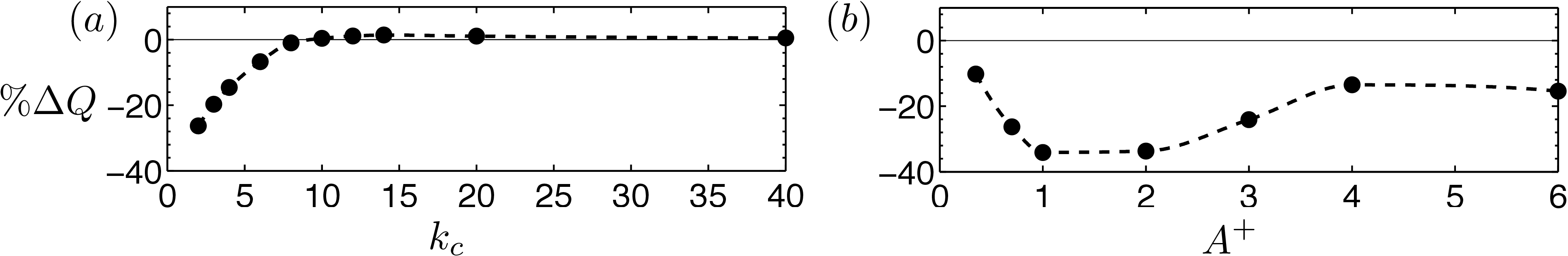
Figure 2: Transpiration effect on the flow rate by changing (a) wavenumber $k_{c}$ at constant amplitude $A^{+}=0.7$ (b) amplitude $A^{+}$ at constant wavenumber $k_{c}=2$.

The independent effects of the two transpiration parameters, $A$ and $k_{c}$, are investigated first. The range of parameters are similar to the one employed by Quadrio et al. (2007) in a channel. Simulations consisting of a parameter sweep while maintaining the other fixed have been carried out at $\mbox{{Re}}_{\tau}=314$. Following the classical Reynolds decomposition, the total velocity has been decomposed as the sum of the mean flow $\bm{u}_{0}$ and a fluctuating velocity $\bm{u}$, which reads

$${\bm{\hat{u}}}(x,r,\theta,t)={\bm{u}}_{0}(x,r)+{\bm{u}}(x,r,\theta,t)\,,$$ (9)

with the mean flow obtained by averaging the total flow in time and the azimuthal direction as

$$\bm{u}_{0}(x,r)=\lim_{T\to\infty}\frac{1}{T}\int_{0}^{T}\frac{1}{2\math@atom{\pi}{\mathchoice{\hbox{$\displaystyle\pi$}}{\hbox{$\textstyle\pi$}}{\hbox{$\scriptstyle\pi$}}{\hbox{$\scriptscriptstyle\pi$}}}}\int_{0}^{2\math@atom{\pi}{\mathchoice{\hbox{$\displaystyle\pi$}}{\hbox{$\textstyle\pi$}}{\hbox{$\scriptstyle\pi$}}{\hbox{$\scriptscriptstyle\pi$}}}}{\bm{\hat{u}}}(x,r,\theta,t)\mathrm{d}t\mathrm{d}\theta\,.$$ (10)

For simplicity in the notation in what follows, we will use $\langle~{}\rangle$ to denote an average in time and azimuthal direction. Hence, $\bm{u}_{0}(x,r)=\langle{\bm{\hat{u}}}\rangle$ .

Note that the streamwise spatial dependence of the mean flow permits a non-zero mean in the wall normal direction, hence $\bm{u}_{0}(x,r)=(u_{0},v_{0},0)$. Turbulence statistics additionally averaged in the streamwise direction are denoted with a bar

$${{\bar{\bm{u}}_{0}}}(r)=\frac{1}{L}\int_{0}^{L}{\bm{u}}_{0}(x,r)\mathrm{d}x\,.$$ (11)

In terms of flow control effectiveness, here we define drag-reducing or drag-increasing configurations as those that reduce or increase the streamwise flow rate with respect to the smooth pipe. Mathematically,

$$\Delta Q=\frac{\int_{0}^{R}{\Delta{\bar{u}_{0}}}r\mathrm{d}r}{\int_{0}^{R}{\bar{u}^{s}_{0}}r\mathrm{d}r}\left\{\begin{array}[]{ll}<0&\mbox{drag-increasing}\,,\\[2.0pt] >0&\mbox{drag-reducing}\,,\end{array}\right.$$ (12)

where $\Delta{u_{0}}=(\bar{u}_{0}^{c}-\bar{u}_{0}^{s})$, being $c$ and $s$ superscripts to denote controlled and smooth pipe respectively. Figure 2(a) shows the percentage variation of the flow rate induced by transpiration with different wavenumber $k_{c}$ at constant amplitude $A^{+}=0.7$, equivalent to $0.22\%$ of the bulk velocity. A large drag increase is observed at small wavenumbers and it asymptotically diminishes until a small increase in flow rate is achieved for $k_{c}\simeq 9$. This small drag reduction slowly lessens and it is observed up to $k_{c}=40$.

Figure 2(b) shows the transpiration influence on the flow rate by increasing the amplitude $A^{+}$ at a constant wavenumber $k_{c}=2$. A drag increase from zero transpiration up to $A^{+}=4$ is observed. The maximum increase is achieved between $A^{+}=1$ and $A^{+}=2$. In agreement with the conjecture posed by Woodcock et al. (2012), increasing the amplitude beyond $A^{+}=4$ does not significantly change the value of the drag increase.

3.1 Comparison with channel flow

We compare our flow control results with the steady streamwise transpiration study of Quadrio et al. (2007) in a channel. The variation of the mean friction coefficient $\Delta C_{f}$ with respect to the smooth pipe is employed to assess the drag reduction/increase. The mean friction coefficient is defined as

$$C_{f}=\frac{2\tau_{w}}{\rho U_{b}^{2}}\,.$$ (13)

Given that the mean wall shear stress is fixed, the mean friction coefficient variation can be expressed solely as function of the ratio between the smooth and controlled pipe bulk velocities, hence

$$\Delta C_{f}=\frac{1}{(1+\Delta Q)^{2}}-1\,.$$ (14)

in which the definition of $\Delta Q$ in (12) is employed. Note that negative values of $\Delta C_{f}$ correspond to drag reduction. Figure 3 shows the comparison of the variation of the friction coefficient versus transpiration wavelength at fixed amplitude $A^{+}=0.7$ in pipe and channel flow. Low and high-$Re$ results are presented for the channel case. Similar behaviour is observed, in which a drag reduction can be achieved in both channel and pipe flows. The maximum friction variation is smaller for the pipe than for the channel. In addition, the rate at which the friction coefficient increases with wavelength is higher for the channel than for the pipe. We note that the manner in which parameters are varied differs between the two studies: while Quadrio et al. (2007) fixed the bulk velocity to arrange a constant bulk Reynolds number during the parameter sweep, here we maintained a constant friction Reynolds number $Re_{\tau}$. It is also worth noting that because of the obvious difference in geometry, identical results are not expected.

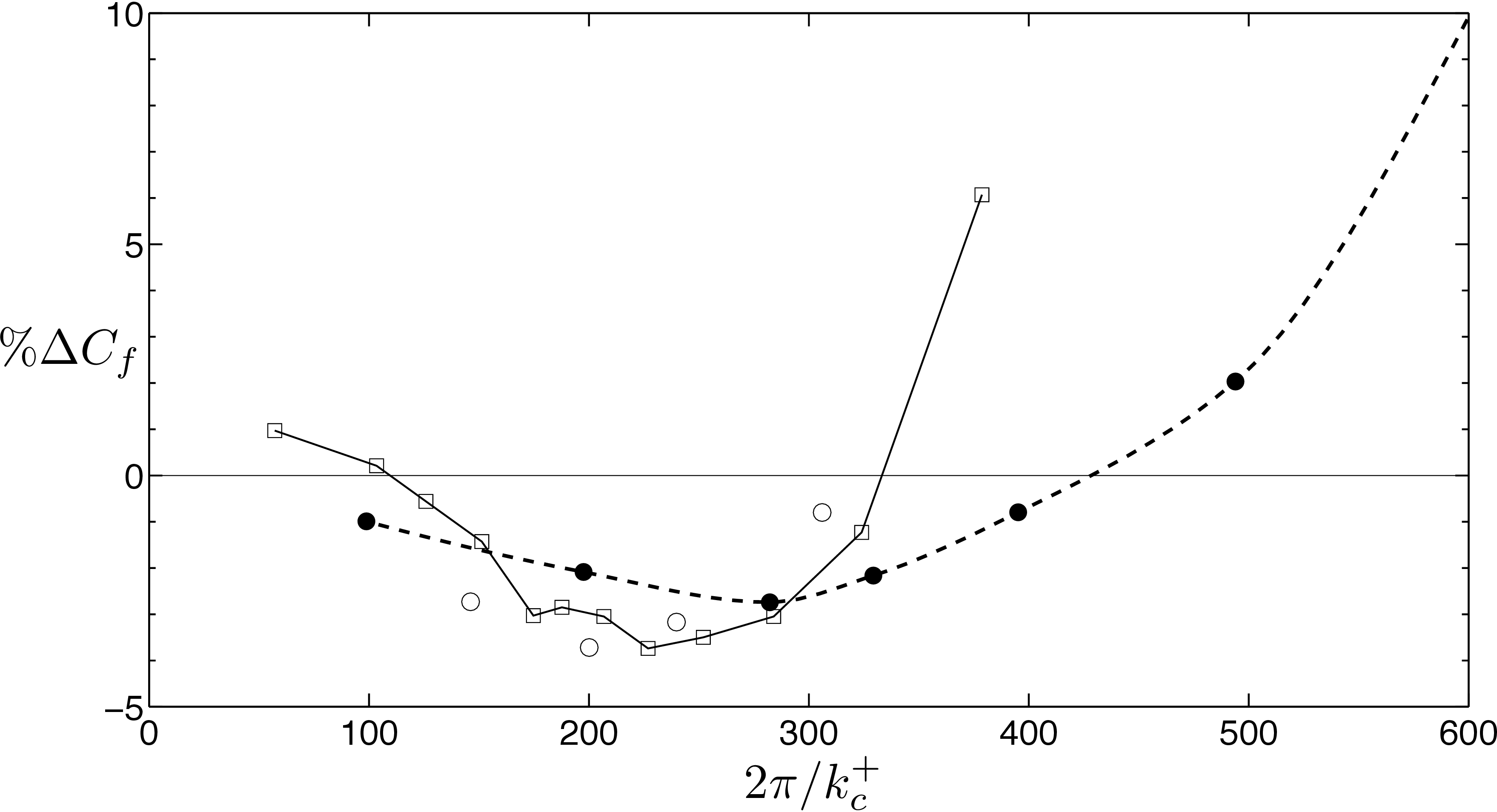
Figure 3: Comparison of the variation of the friction coefficient versus transpiration wavelength at fixed amplitude $A^{+}=0.7$. Solid circles, pipe flow at $Re_{\tau}=314$ (present results); open circles, channel flow at $Re_{\tau}=400$ (Quadrio et al., 2007); squares, channel flow at $Re_{\tau}=180$ (Quadrio et al., 2007).

4 Turbulence statistics

4.1 Constant transpiration amplitude

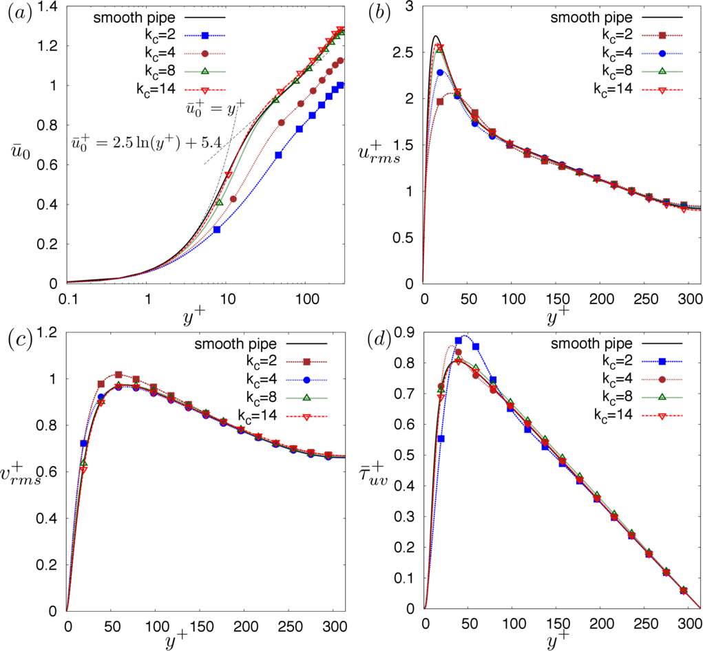
Figure 4: Comparison of profile data for the smooth-wall pipe (solid line) and pipe with transpiration at constant amplitude $A^{+}=0.7$ and different wavenumbers $k_{c}$. (a), mean flow normalized by $U_{b}$, with dashed lines for linear sublayer and fitted log law; (b), axial turbulent intensity; (c), radial turbulent intensity; (d), Reynolds shear stress.

The effect of transpiration is evident in the behaviour of the mean velocity characteristics. Figure 4(a) shows the effect of changing the transpiration wavenumber $k_{c}$ at a small constant amplitude $A^{+}=0.7$ on the mean streamwise velocity $\bar{u}_{0}(r)$ compared to the smooth pipe. Additionally, dashed lines for the linear sublayer and fitted log law (den Toonder & Nieuwstadt, 1997) are shown as reference. In agreement with figure 2(a), we observe reduced flow rates in figure 4(a) for $k_{c}<8$ with a small increase occurring around $k_{c}=10$. Two interesting features are noticed. First, the viscous sublayer is no longer linear. Since the mean wall-shear $\tau_{w}$ is constant, all the profiles must collapse as $y^{+}=(R^{+}-r^{+})$ approaches zero. In other words, the value of ${\partial u_{0}}/{\partial y}$ at the wall is the same for all cases considered.

Second, the outer-layer of all the profiles are parallel, suggesting that the overlap region can be expressed as

$$\bar{u}_{0}^{+}=2.5\ln(y^{+})+5.4+\Delta T^{+}\,,$$ (15)

with the transpiration factor, $\Delta T$ arising in a similar way as the roughness factor of Hama (1954), or the corrugation factor of Saha et al. (2015b). However, we note that the present Reynolds number may not be sufficiently high for the emergence of a self-similar log law in the overlap region. Although there is not a well-defined log layer at such low Re, we could refer to it as log layer for convenience. The present results suggest what will happen at a greater Re. Figure 5 shows a defect velocity scaling of the mean profiles. A collapse of the mean velocity profiles is observed in the outer layer, hence Townsend’s wall similarity hypothesis (Townsend, 1976) applies in the present low amplitude transpiration cases.

Figure 4(b) and (c) show the influence of the transpiration on the turbulent intensities, presented as root mean squares. At this small amplitude, the transpiration mainly affects the location and value of the maximum turbulent intensities and all profiles collapse as $y^{+}$ approaches the centerline, indicating that small amplitude transpiration does not alter the turbulent activity in the outer layer. Note that the peak in axial turbulent intensity moves due to the reduction in shear at the same wall-normal location in all the cases, which is apparent in the man velocity profiles in Fig. 4(a).

Figure 4(d) shows that the influence of small amplitude transpiration on the Reynolds shear stress $\tau_{uv}=\langle u^{c}v^{c}\rangle$. We observed that the transpiration influence on $\tau_{uv}$ is only significant at small wavenumbers and, as with the turbulent intensities, small amplitude transpiration does not change the outer layer of the profile. The small changes in the shear stress are not enough to explain the significant variations in the mean flow, hence it is inferred that additional effects related to steady streaming and non-zero mean streamwise gradients play a major role in the momentum balance.

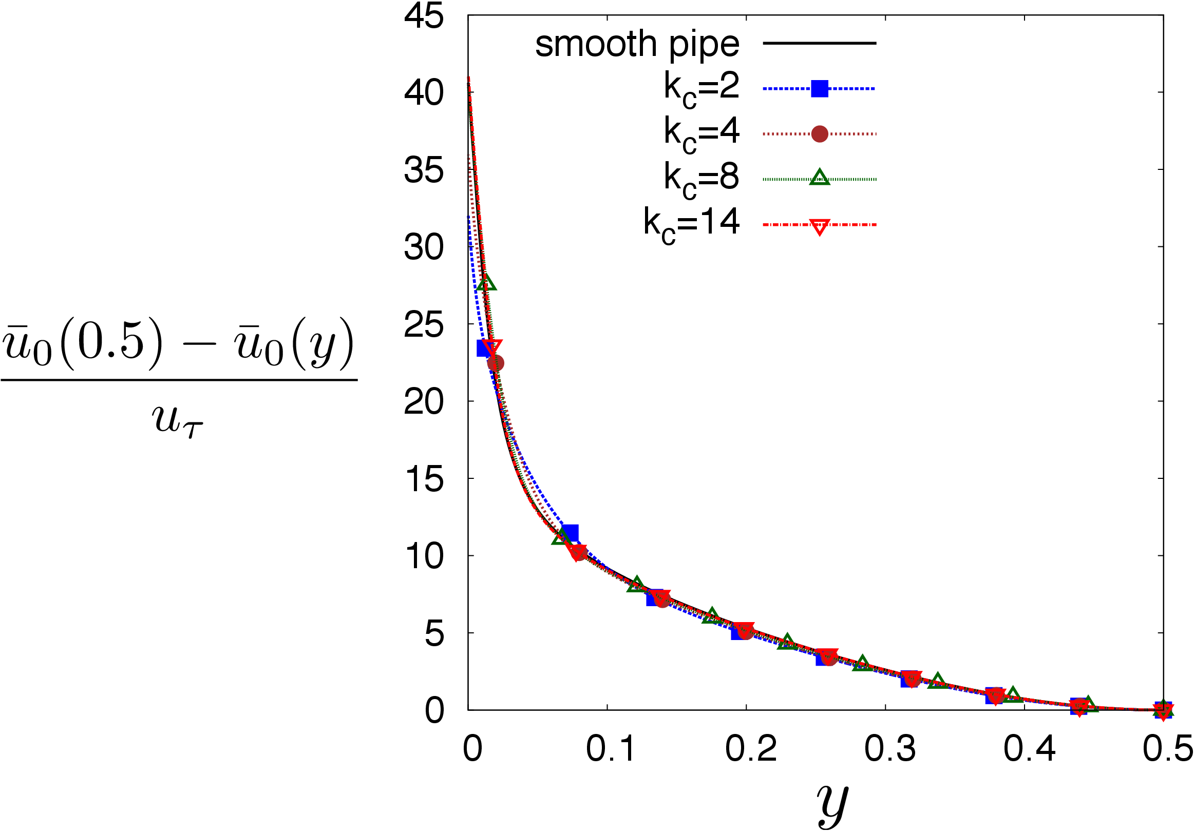
Figure 5: Defect velocity law for profile data of the smooth-wall pipe (solid line) and pipe with transpiration at constant amplitude $A^{+}=0.7$ and different wavenumbers $k_{c}$. A collapse of all the mean velocity profiles is observed in the outer layer hence small amplitude effects do not alter the turbulent activity in the outer layer.

Figure 6: Comparison of profile data for the smooth-wall pipe (solid line) and pipe with transpiration at constant wavenumber $k_{c}=2$ and different amplitudes $A^{+}$. (a), mean flow normalized by $U_{b}$, with dashed lines for linear sublayer and fitted log law; (b), axial turbulent intensity; (c), radial turbulent intensity; (d), Reynolds shear stress.

4.2 Constant transpiration wavenumber

The effect of changing the amplitude $A^{+}$ at a constant forcing wavenumber $k_{c}=2$ in the mean streamwise velocity $u_{0}$ is shown in figure 6(a). For $A^{+}<2$, results are similar to those observed for small amplitudes. At $A^{+}=2$ the flow rate is dramatically decreased and the overlap region is reduced compared to the small amplitude cases. At $A^{+}=4$ the parallel overlap region is not existent. This large amplitude can significantly increase the mean velocity in the outer layer. Similarly, we observe that large amplitude transpiration shifts the location of maximum turbulent intensities towards the centerline, as seen in Figures 6(b) and (c). We can state that large amplitudes $A^{+}>2$ can influence the turbulent activity in the outer layer. Figure 6(d) shows that high amplitudes have a similar effect on the shear stress and how a high amplitude $A^{+}=4$ can dramatically reduce the Reynolds shear stress and shift the location of the maximum towards the centerline.

These tendencies in $A^{+}$ and $k_{c}$ suggest that very high values of the transpiration amplitude combined with high wavenumber $k_{c}$ can be explored in order to find significant drag-reducing configuration. This has been confirmed through the investigation of a static transpiration case with an amplitude $A^{+}=10$ and wavenumber $k_{c}=10$, yielding an increase in flow rate of $\Delta Q=19.3\%$. This case will be investigated in detail in the next section.

5 Streamwise momentum balance

As previously mentioned, we have inferred from figures 4 and 6 that the changes in Reynolds stress are not enough to explain the changes in the mean velocity profile; additional effects related to steady streaming and non-zero mean streamwise gradients could play a major role in the momentum balance. Here we analyze the streamwise momentum balance in order to identify these additional effects. The axial momentum equation averaged in time and azimuthal direction for a pipe flow controlled with static transpiration is

$$f_{x}+\frac{1}{r}\frac{\partial}{\partial{r}}(-r\tau_{uv}^{c}-ru^{c}_{0}v^{c}_{0}+r\mbox{{Re}}_{s}^{-1}\frac{\partial{u^{c}_{0}}}{\partial{r}})+\mathcal{N}_{x}=0\,.$$ (16)

with $\mathcal{N}_{x}$ being the sum of terms with $x-$derivatives, representing the non-homogeneity of the flow in the streamwise direction (Fukagata et al., 2002).

$$\mathcal{N}_{x}=\frac{\partial(u_{0}^{c}u_{0}^{c})}{\partial x}+\frac{\partial\langle u^{c}u^{c}\rangle}{\partial x}-\mbox{{Re}}_{s}^{-1}\frac{\partial^{2}u_{0}^{c}}{\partial x^{2}}\,.$$ (17)

where $\langle\rangle$ denotes averaging in time and the azimuthal direction. Equation (16) for a smooth pipe yields

$$f_{x}+\frac{1}{r}\frac{\partial}{\partial{r}}(-r\tau_{uv}^{s}+r\mbox{{Re}}_{s}^{-1}\frac{\partial{u^{s}_{0}}}{\partial{r}})=0\,,$$ (18)

Since the body force $f_{x}$ and Reynolds number $\mbox{{Re}}_{s}^{-1}$ have the same value in (16) and (18), these two equations can be subtracted and integrated in the wall normal direction to give

$$\mbox{{Re}}_{s}^{-1}{\Delta{u_{0}}(x,r)}=\int_{0}^{r}\Delta{\tau}r^{\prime}\mathrm{d}r^{\prime}+\int_{0}^{r}u^{c}_{0}v^{c}_{0}r^{\prime}\mathrm{d}r^{\prime}+\int_{0}^{r}\mathcal{N}^{\prime}_{x}r^{\prime}\mathrm{d}r^{\prime}\,,$$ (19)

in which $\mathcal{N}_{x}$ has been previously integrated with respect to the wall normal direction to yield $\mathcal{N}^{\prime}_{x}$. This equation can be additionally averaged in the axial direction to identify three different terms playing a role in the modification of the mean profile

$$\Delta{\bar{u}_{0}}(r)=RSS+ST+NH\,,$$ (20)

where

$$RSS(r) = \frac{-\mbox{{Re}}_{s}}{L}\int_{0}^{L}\int_{0}^{r}\Delta{\tau}r^{\prime}\mathrm{d}r^{\prime}\mathrm{d}x\,,$$ (21)

$$ST(r) = \frac{-\mbox{{Re}}_{s}}{L}\int_{0}^{L}\int_{0}^{r}u^{c}_{0}v^{c}_{0}r^{\prime}\mathrm{d}r^{\prime}\mathrm{d}x\,,$$ (22)

$$NH(r) = \frac{\mbox{{Re}}_{s}}{L}\int_{0}^{L}\int_{0}^{r}\mathcal{N}^{\prime}_{x}r^{\prime}\mathrm{d}r^{\prime}\,\mathrm{d}x\,.$$ (23)

The first term $RSS$ represents the interaction of the transpiration with the Reynolds shear stress, and its behaviour can be inferred from the turbulence statistics shown in Figures 4(d) and 6(d). The second term $ST$ is associated with the steady streaming produced by the static transpiration. As briefly mentioned in the introduction, this term defined in (22) consists of an additional flow rate due to the interaction of the wall-normal transpiration with the flow convecting downstream (Luchini, 2008). This term can be alternatively understood as a coherent Reynolds shear stress. The velocity averaged in time and azimuthal direction defined in (10) can be decomposed into a mean profile ${{\bar{\bm{u}}_{0}}}(r)$ and a steady deviation from that mean velocity profile $\bm{u}_{0}^{\prime}(x,r)$

$$\bm{u}_{0}(x,r)={{\bar{\bm{u}}_{0}}}(r)+{\bm{u}}_{0}^{\prime}(x,r)\,.$$ (24)

Taking into account this decomposition, the integrand of the steady streaming term now reads

$$u^{c}_{0}v^{c}_{0}={{\bar{u}^{c}_{0}}}{{\bar{v}^{c}_{0}}}+{{\bar{u}^{c}_{0}}}{v^{c}_{0}}^{\prime}\,+{{\bar{v}^{c}_{0}}}{u^{c}_{0}}^{\prime}\,+{u^{c}_{0}}^{\prime}{v^{c}_{0}}^{\prime}\,.$$ (25)

and its axial average is reduced to

$$\frac{1}{L}\int_{0}^{L}u^{c}_{0}v^{c}_{0}\mathrm{d}x=\frac{1}{L}\int_{0}^{L}{u^{c}_{0}}^{\prime}{v^{c}_{0}}^{\prime}\mathrm{d}x\,,$$ (26)

since ${{\bar{v}^{c}_{0}}}$ must be zero because of the continuity equation. Hence the steady streaming term $ST$ is generated by coherent Reynolds shear stress induced by the deviation of the velocity from the axial mean profile. We highlight that the substitution of the decomposition (33) in the Reynolds decomposition in (9) leads to a triple decomposition, in which the deviation from the mean velocity profile plays the role of a coherent velocity fluctuation.

The third term $NH$ defined in (23) corresponds to the axial non-homogeneity in the flow induced by the transpiration. It consists of non-zero mean streamwise gradients generated by the transpiration. Because of the low amplitudes considered in previous works (Quadrio et al., 2007), this last term has not been isolated before and has been implicitly absorbed in an interaction with turbulence term that accounts for both $ST$ and $NH$ terms.

Finally, we note that the identity derived by Fukagata et al. (2002) (FIK identity) could be alternatively employed for our analysis. However, the difference in bulk flow Reynolds numbers between uncontrolled and controlled cases favors the present approach.

5.1 Representative transpiration configurations

The relative importance of the three terms acting in the transpiration is investigated by inspecting three representative transpiration configurations in terms of drag modification. Table 1 lists the contributions to the change in flow rate of these configurations: (I) the largest drag-reducing case found ($\Delta Q=19.3\%$) consisting of a large amplitude and transpiration wavenumber $(A^{+},k_{c})=(10,10)$, (II) a small drag-reducing case ($\Delta Q=0.4\%$) induced by a tiny amplitude at a large wavenumber $(A^{+},k_{c})=(0.7,10)$, and (III) a large drag-increasing case ($\Delta Q=-36.1\%$) with small wavenumber and amplitude $(A^{+},k_{c})=(2,2)$.

We first compare the Reynolds shear stress generated by the fluctuating velocity $\tau_{uv}$ and the shear stress arising from the deviation velocity ${u^{c}_{0}}^{\prime}{v^{c}_{0}}^{\prime}$. The radial distributions of the three different cases are showed in figure 7. We observe that the streaming or coherent Reynolds shear stress is dominant close to the wall and opposes the Reynolds stress generated by the fluctuating velocity. Far from the wall, the Reynolds stress is governed by the fluctuating velocity.

		$A^{+}$	$k_{c}$	$\Delta Q(\%)$	$\int RSS(\%)$	$\int ST(\%)$	$\int NH(\%)$
(I)	large drag-reduction	10	10	19.3	28.4	$-20.4$	11.3
(II)	small drag-reduction	0.7	10	0.4	1.5	$-1.7$	0.6
(III)	drag-increase	2	2	$-36.1$	11.2	$-29.6$	$-17.7$

Table 1: Contributions to the change in flow rate of different transpiration configurations based on integration of Equation (20)($\int$ denotes integration in wall normal direction).

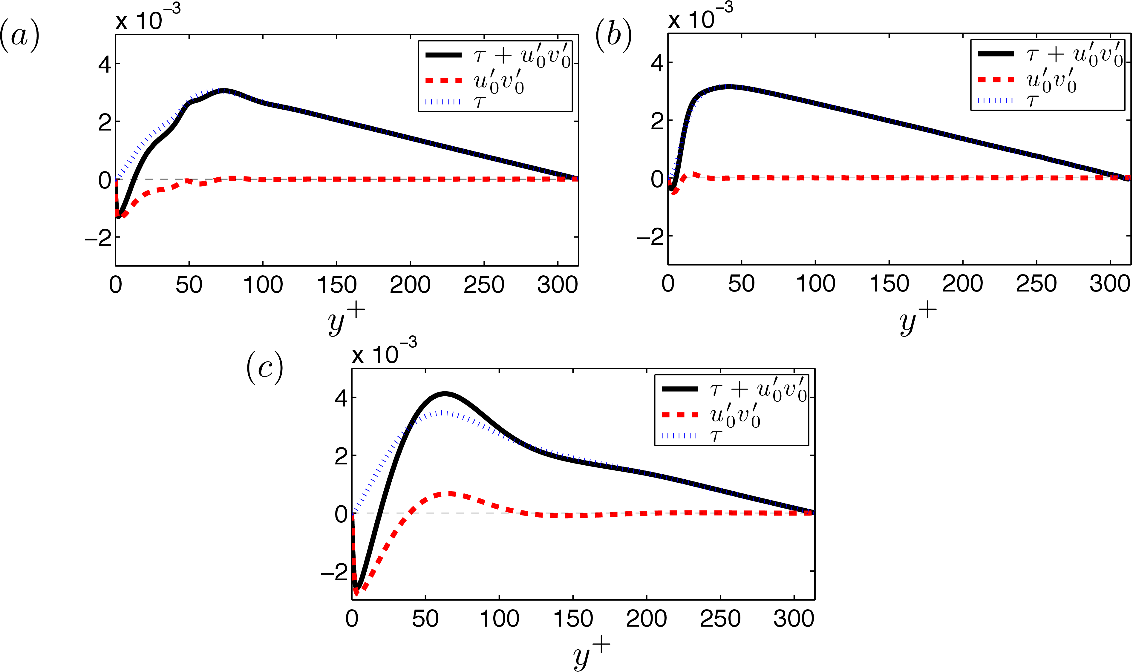
Figure 7: Radial distribution of the Reynolds shear stress generated by the fluctuating velocity $\tau_{uv}$ and the deviation velocity ${u^{c}_{0}}^{\prime}{v^{c}_{0}}^{\prime}$ (a) case I: large drag-decrease $(A^{+},k_{c})=(10,10)$, (b) case II: small drag-decrease $(A^{+},k_{c})=(0.7,10)$, (c) case III: drag-increase $(A^{+},k_{c})=(2,2)$.

Figure 8 shows the radial profile of the different contributions to the mean profile and figure 9 the corresponding mean profiles of the cases considered. Figure 8(a) corresponds to the drag-decrease case $(A^{+},k_{c})=(10,10)$. It can be observed that the contributions to the increase in flow rate are caused by a large reduction of Reynolds shear stress (28.4%) and the streamwise gradients produced in the flow at such large amplitude and wavenumber (11.3%). However, these contributions are mitigated by the opposite flow rate induced by the steady streaming ($-20.4\%$). Figure 8(b) corresponds to a low amplitude static transpiration $A^{+}=0.7$ at the same axial wavenumber as case (b), yielding a very small reduction in flow rate. Similarly, the effect on the Reynolds shear stress (1.5%) and the non-homogeneity effects (0.6%) contribute to increase the flow rate while the streaming produced is opposite to the mean flow, but of a lesser magnitude ($-1.7\%$). Figure 8(c) represents the drag-increase case $(A^{+},k_{c})=(2,2)$. As opposed to the two previous cases, the main contribution to the drag is caused by a large steady streaming in conjunction with a large non-zero streamwise gradients opposite to the mean flow. Although the decrease in Reynolds stress is significant and favorable towards a flow rate increase, the sum of the other two terms is much larger. In terms of the variation of mean profile, we observe a similar behaviour in all cases: there is a decrease in the mean streamwise velocity profile close to the wall induced by the streaming term or coherent Reynolds shear stress. Within the buffer layer, the difference in mean velocity decreases until a minimum is achieved and then it increases to a maximum in the overlapping region. A smooth decrease towards the centerline is then observed.

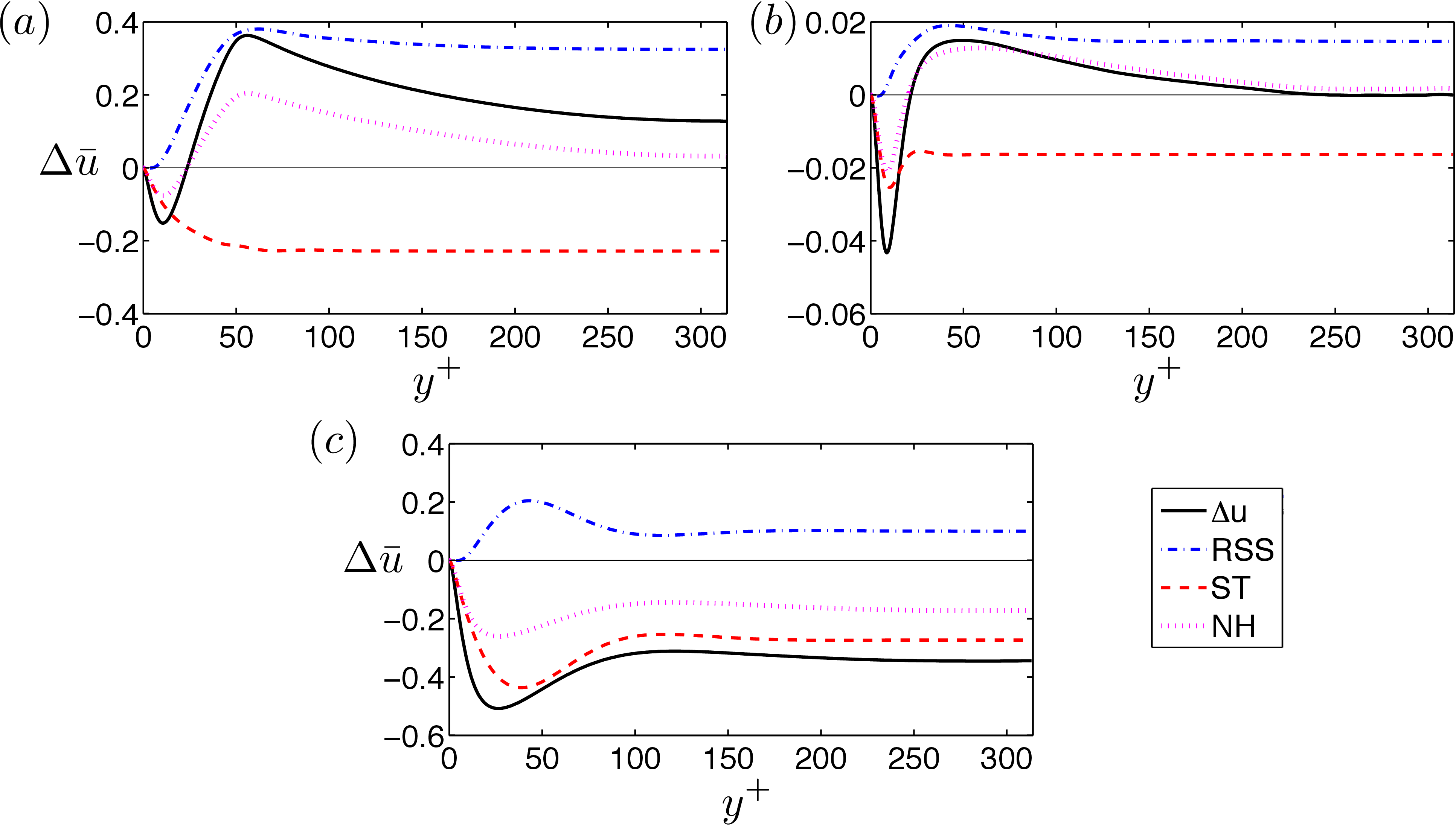
Figure 8: Radial distribution of the different terms in (20) to the streamwise momentum balance. Solid line $\Delta{\bar{u}_{0}}(r)$; -$\cdot$- Reynolds shear stress term$RSS$; $--$ steady streaming terms $ST$; $\cdot$$\cdot$$\cdot$$\cdot$ non-homogeneous terms $NH$. (a) case I: large drag-decrease $(A^{+},k_{c})=(10,10)$, (b) case II: small drag-decrease $(A^{+},k_{c})=(0.7,10)$, (c) case III: drag-increase $(A^{+},k_{c})=(2,2)$.

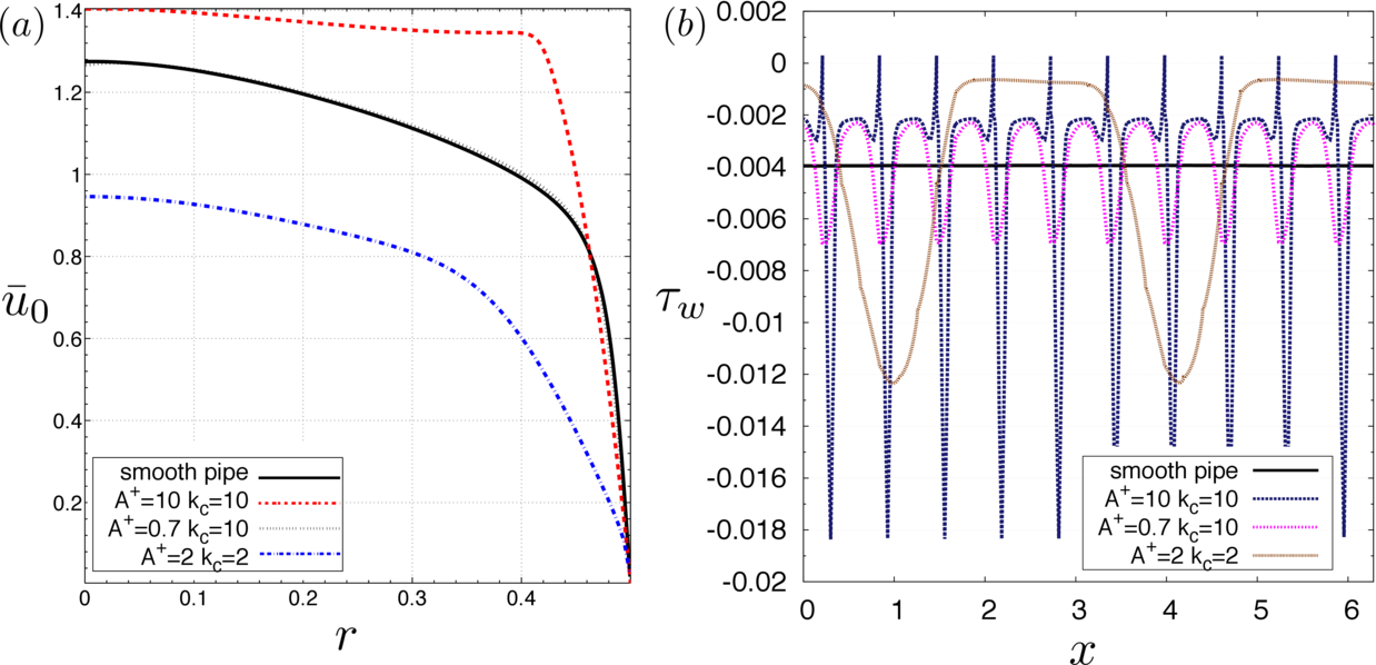
Figure 9: (a) Streamwise mean profile (b) Mean wall shear along the axial direction

Streamlines and kinetic energy of the two-dimensional mean velocities $\bm{u}_{0}(x,r)$ are shown in figure 10. Preceding the analysis of the flow dynamics, we observe that blowing is associated with areas of high kinetic energy while suction areas slow down the flow. Despite the large amplitudes employed, we observe an apparent absence of recirculation areas in these mean flows. Figure 9(b) shows the mean wall shear along the axial direction. Only a very small flow separation occurs in the large drag-decrease $(A^{+},k_{c})=(10,10)$. Hence flow separation effects are not associated with the observed drag modifications.

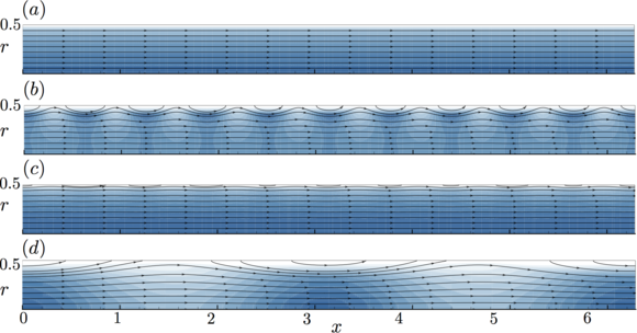
Figure 10: Two-dimensional mean flow: streamlines and normalized kinetic energy for each different case (white to blue) ($a$) reference case: smooth pipe ($b$) drag-reducing case $(A^{+},k_{c})=(10,10)$ ($c$) neutral case $(A^{+},k_{c})=(0.7,10)$ ($d$) drag-increasing case $(A^{+},k_{c})=(2,2)$

5.2 Flow control energetic performance

As stated by Quadrio (2011), a flow control system study must always be accompanied with its respective energetic perfomance analysis in order to determine its validity in real applications. The control performance indices in the sense of Kasagi et al. (2009) are employed here to assess the energy effectiveness of the transpiration. We define a drag reduction rate as

$$W=(P_{c}-P_{s})/{P_{s}}\,,$$ (27)

where $P$ is the power required to drive the pipe flow and the subscripts $c$ and $s$ refer again to controlled and smooth pipe. The index $W$ can also be interpreted as the proportional change in the power developed by the constant body force $f_{x}$ as a consequence of the transpiration. Note from (27) and (28) that the drag reduction rate $W$ is equivalent to the flow rate variation $\Delta Q$. The power required to drive the flow is given by the product of the body force times the bulk velocity

$$P=f_{x}\math@atom{\pi}{\mathchoice{\hbox{$\displaystyle\pi$}}{\hbox{$\textstyle\pi$}}{\hbox{$\scriptstyle\pi$}}{\hbox{$\scriptscriptstyle\pi$}}}R^{2}LU_{b}\,.$$ (28)

A net energy saving rate $S$ is defined to take into account the power required to operate the flow control

$$S=\left(P_{s}-(P_{c}+P_{in})\right)/{P_{s}}\,.$$ (29)

The mean flow momentum and energy equation are employed to obtain the power required to apply the transpiration control, as also done by Marusic et al. (2007) and Mao et al. (2015). The power employed to apply the transpiration control reads

$$P_{in}=\int_{0}^{2\math@atom{\pi}{\mathchoice{\hbox{$\displaystyle\pi$}}{\hbox{$\textstyle\pi$}}{\hbox{$\scriptstyle\pi$}}{\hbox{$\scriptscriptstyle\pi$}}}}\int_{0}^{L}\left(\frac{1}{2}v_{0}(x,R)^{3}+p(x,R)v_{0}(x,R)\right)\,\mathrm{d}xR\mathrm{d}\theta.$$ (30)

with $v_{0}(x,R)=A\sin(k_{c}x)$. The first term in the integral represents the rate at which energy is introduced or removed as kinetic energy in the flow through the pipe wall. This term is exactly zero because the change of net mass flux is zero and the velocity is sinusoidal, imposed by the transpiration boundary condition in (3). The second term represents the rate of energy expenditure by pumping flow against the local pressure at the wall. Finally, the effectiveness of the transpiration control is defined as the ratio between the change in pumping power and power required to apply the transpiration control, which reads

$$G=(P_{s}-P_{c})/P_{in}\,.$$ (31)

Note that the net power saving can be alternatively written as

$$S=W(1-G^{-1})\,,$$ (32)

which indicates that an effectiveness $G$ higher than one is required for a positive power gain. As reported by Kasagi et al. (2009), typical maxima for active feedback control systems are in the range of $G\sim 100$ and $S\sim 0.15$ and for predetermined control strategies, such as spanwise wall-oscillation control in channel (Quadrio & Ricco, 2004) or streamwise travelling transpiration in channel (Min et al., 2006), a range of $2\lesssim G\lesssim 6$ and $0.05\lesssim S\lesssim 0.25$ was found.

	$A^{+}$	$k_{c}$	$W$	$G$	$S$
(I) large drag-reduction	10	10	0.19	1.02	0.004
(II) small drag-reduction	0.7	10	0.04	0.21	-0.014
(III) drag-increase	2	2	-0.36	-3.73	-0.46

Table 2: Flow control energetic performance indices. $W$ represents the drag reduction rate, $G$ the effectiveness of the transpiration control and $S$ the net energy saving rate.

The resulting flow control energetic performance indices are listed in table 2. Note that the change in pumping power rate $W$ is equivalent to the flow rate variation $\Delta Q$. Despite the large drag reduction produced by the configuration $(A^{+},k_{c})=(10,10)$, the net energy saving rate is marginal and the small drag reduction caused at $(A^{+},k_{c})=(0.7,10)$ has an effectiveness less than one, with a net energy expenditure. The case $(A^{+},k_{c})=(2,2)$ is interesting, as it shows a high effectiveness in decreasing the flow rate and has the potential to relaminarize the flow at lower $Re_{\tau}$. For instance, a reduction in flow rate $\Delta Q=-36\%$ at $Re_{\tau}=115$ could reduce the critical bulk flow Reynolds below $Re<2040$ and thus achieve a relaminarization of the flow. Finally, we remark that the particular case $(A^{+},k_{c})=(10,10)$ is probably not the globally optimal configuration for steady transpiration and net energy saving rates and effectiveness in the range of typical values for the flow control strategies reported by Kasagi et al. (2009) might be possible, if the full parameter space was considered.

6 Flow dynamics

As a first step in establishing a relationship between changes in flow structures and drag reduction or increase mechanisms, this section describes how the most amplified and energetic flow structures are affected by the transpiration.

6.1 Resolvent analysis

The loss of spatial homogeneity in the axial direction is the main challenge when incorporating transpiration effects into the resolvent model. One solution is to employ the two-dimensional resolvent framework of Gómez et al. (2014). This method is able to deal with flows in which the mean is spatially non-homogeneous. The dependence on the axial coordinate $x$ is retained in the formulation, in contrast with the classical one-dimensional resolvent formulation of McKeon & Sharma (2010). However, the method leads to a singular value decomposition problem with storage requirements of order $\mathcal{O}(N_{r}^{2}N_{x}^{2})$, with $N_{r}$ and $N_{x}$ being the resolution in the radial and axial directions respectively, as opposed to the original formulation which was of order $N_{r}^{2}$. Consequently, the two-dimensional method is not practical for a parameter sweep owing to the large computational effort required. In the following we present a computationally cheaper and simple alternative based on a triple decomposition of the total velocity.

Based on the decompositions in (9) and (33), the total velocity is decomposed as a sum of the axial mean profile, a steady but spatially varying deviation from the axial profile and a fluctuating velocity

$$\bm{\hat{u}}(x,r,\theta,t)=\bar{\bm{u}}(r)+\bm{u}^{\prime}(x,r)+\bm{u}(x,r,\theta,t).$$ (33)

The fluctuating velocity is expressed as a sum of Fourier modes. These are discrete since the domain has a fixed periodic length and is periodic in the azimuth:

$$\bm{\hat{u}}(x,r,\theta,t)=\bar{\bm{u}}(r)+\bm{u}_{l}^{\prime}(r)\mathrm{e}^{\mathrm{i}lx}+\sum_{(k,n,\omega)\neq(l,0,0)}\bm{u}_{k,n,\omega}(r)\mathrm{e}^{\mathrm{i}(kx+n\theta-\omega t)}+\mathrm{c.c.},$$ (34)

where $k$, $n$ and $\omega$ are the axial, azimuthal wavenumber and the temporal frequency, respectively. Note than a complex-conjugate must be added because $\bm{\hat{u}}$ is real.

Without loss of generality, we have assumed that the deviation velocity can be expressed as a single Fourier mode with axial wavenumber $l$. As a consequence of the triadic interaction between the spatial Fourier mode of the deviation velocity and the fluctuating velocity, there is a coupling of the fluctuating velocity at $(k,n,\omega)$ with that at $(k\pm l,n,\omega)$ (see Appendix A). Similarly, the non-linear forcing terms generated by the fluctuating velocity are written as $\bm{f}_{k,n,\omega}=(\bm{u\cdot\nabla u})_{k,n,\omega}$.

Taking (33) into account, it follows that the Fourier-transformed Navier–Stokes equation (2) yields the linear relation

$$\bm{u}_{k,n,\omega}=\mathcal{H}_{k,n,\omega}\left(\bm{f}_{k,n,\omega}+\mathcal{C}_{k,n,\omega}\bm{u}_{k\pm l,n,\omega}\right)\,$$ (35)

for $(k,n,\omega)\neq(0,0,0)$ and $(k,n,\omega)\neq(\pm l,0,0)$, where $\mathcal{C}_{k,n,\omega}$ is a coupling operator representing the triadic interaction between deviation and fluctuating velocity. The triadic interaction can be considered as another unknown forcing and it permits lumping all forcing terms as

$$\bm{g}_{k,n,\omega}=\bm{f}_{k,n,\omega}+\mathcal{C}_{k,n,\omega}\bm{u}_{k\pm l,n,\omega}\,,$$ (36)

hence the following linear velocity–forcing relation is obtained

$$\bm{u}_{k,n,\omega}=\mathcal{H}_{k,n,\omega}\bm{g}_{k,n,\omega}\,.$$ (37)

The resolvent operator $\mathcal{H}_{k,n,\omega}$ acts as a transfer function between the fluctuating velocity and the forcing of the non-linear terms, thus it provides information on which combination of frequencies and wavenumber are damped/excited by wall transpiration effects. Equation (38) shows the resolvent $\mathcal{{H}}_{k,n,\omega}$. The first, second and third rows corresponds to the streamwise, wall-normal and azimuthal momentum equation, respectively.

$$\mathcal{{H}}_{k,n,\omega}(r)=\left[\begin{array}[]{ccc}\mathrm{i}(ku_{0}-\omega)-\mbox{{Re}}^{-1}(D+r^{-2})&\partial_{r}{u_{0}}&0\\ 0&\mathrm{i}(ku_{0}-\omega)-Re^{-1}D&-2\mathrm{i}nr^{-2}\mbox{{Re}}^{-1}\\ 0&-2\mathrm{i}nr^{-2}\mbox{{Re}}^{-1}&\mathrm{i}(ku_{0}-\omega)-\mbox{{Re}}^{-1}D\\ \end{array}\right]^{-1},$$ (38)

with

$$D=-k^{2}-(n^{2}+1)r^{-2}+\partial^{2}_{r}+r^{-1}\partial_{r}\,.$$ (39)

The physical interpretation of the present resolvent formulation is the same to that of the original formulation (McKeon & Sharma, 2010). Figure 11 presents the new resolvent formulation (37) by means of a block diagram. The mean velocity profile is sustained in the $(k,n,\omega)=(0,0,0)$ equation via the Reynolds stress $f_{0,0,0}$ and interactions with deviation velocity. Similarly, the deviation velocity is also sustained via the forcing $f_{l,0,0}$ and interactions with the mean flow in the mean flow equation corresponding to $(k,n,\omega)=(l,0,0)$. The deviation velocity drives the triadic interactions generated via the operator $\mathcal{C}_{k,n,\omega}$ and, closing the loop, the mean profile restricts how the fluctuating velocity responds to the non-linear forcing via the resolvent operator $\mathcal{H}_{k,n,\omega}$. We note that it is relatively straightforward to generalize the block diagram in figure 11 if the deviation velocity is composed of multiple axial wavenumbers, or even frequencies.

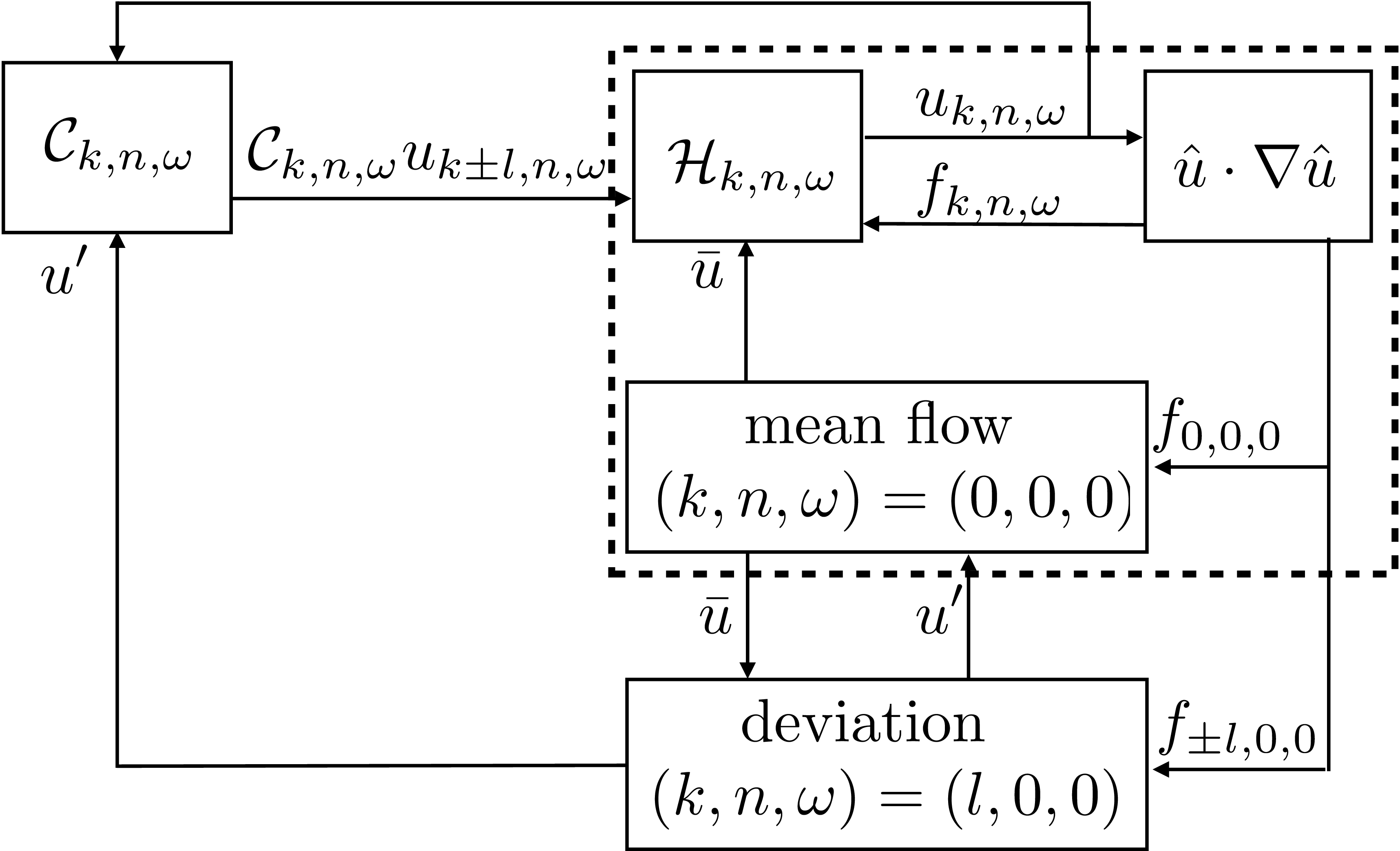
Figure 11: Diagram of the new triple-decomposition-based resolvent model. The mean velocity profile is sustained in the $(k,n,\omega)=(0,0,0)$ equation via the Reynolds stress $f_{0,0,0}$ and the interactions with deviation velocity. Similarly, the deviation velocity is also sustained via the forcing $f_{l,0,0}$ and interactions with the mean flow in the $(k,n,\omega)=(l,0,0)$ equation. The original model of McKeon & Sharma (2010) is represented by the subset within the dashed border.

We highlight that this formulation represents the exact route for modifying a turbulent flow using the mean profile $u_{0}$. Despite the non-homogeneity of the flow in our present cases of interest, the operator $\mathcal{H}_{k,n,\omega}$ is identical to the one developed by McKeon & Sharma (2010) for one-dimensional mean flows and thus it only depends on the axial mean $\bar{u}(r)$; the deviation velocity does not appear in the resolvent, but it does appear in the mean flow equation. Also note that the equation of continuity enforces the condition that the mean profile of wall-normal velocity $v_{0}$ is zero in all cases. Hence the modification of the mean profile $\bar{u}_{0}$ is sufficient to analyze the dynamics of the flow. We recall that McKeon et al. (2013) used a comparable decomposition in order to assess the effect of a synthetic large-scale motion on the flow dynamics.

Following the analysis of McKeon & Sharma (2010), a singular value decomposition (SVD) of the resolvent operator

$$\mathcal{H}_{k,n,\omega}=\sum_{m}{\bm{\psi}}_{k,n,\omega,m}\sigma_{k,n,\omega,m}{\bm{\phi}}^{*}_{k,n,\omega,m}$$ (40)

delivers an input-output amplification relation between response modes $\bm{\psi}_{k,n,\omega,m}$ and forcing modes $\bm{\phi}_{k,n,\omega,m}$ through the magnitude of the corresponding singular value $\sigma_{k,n,\omega,m}$. Here the subscript $m$ is an index that ranks singular values from largest to smallest. The non-linear terms $\bm{g}_{k,n,\omega}$ can be decomposed as a sum of forcing modes to relate the amplification mechanisms to the velocity fields,

$$\bm{g}_{k,n,\omega}=\sum_{m}\chi_{k,n,\omega,m}\bm{\phi}_{k,n,\omega,m}$$ (41)

where the unknown forcing coefficients $\chi_{n,\omega,n}$ represent the unknown mode interactions and Reynolds stresses. The decomposition of the fluctuating velocity field is then constructed as a weighted sum of response modes

$$\bm{u}(x,r,\theta,t)=\sum_{(k,n,\omega)\neq(l,0,0)}\chi_{k,n,\omega,1}\sigma_{k,n,\omega,1}\bm{\psi}_{k,n,\omega,1}\mathrm{e}^{\mathrm{i}(kx+n\theta-\omega{t})}\,,$$ (42)

in which the low-rank nature of the resolvent, $\sigma_{k,n,\omega,1}\gg\sigma_{k,n,\omega,2}$, is exploited (McKeon & Sharma, 2010; Sharma & McKeon, 2013; Luhar et al., 2014).

A numerical method similar to the one developed by McKeon & Sharma (2010) is employed for the discretization of the resolvent operator $\mathcal{H}_{k,n,\omega}$. Following the approach of Meseguer & Trefethen (2003), wall normal derivatives are computed using Chebychev differentiation matrices, properly modified to avoid the axis singularity. Notice that instead of projecting the velocity into a divergence-free basis, here the divergence-free velocity fields are enforced by adding the continuity equation as an additional column and row in the discretized resolvent (Luhar et al., 2014). The velocity boundary conditions at the wall are zero Dirichlet. The velocity profile inputs of the four cases subject to study were shown in figure 9.

6.2 Fourier analyses and DMD

It may be observed in (42) that the energy associated with each Fourier mode ${\bm{u}}_{k,n,\omega}$ is proportional to its weighting $\chi_{k,n,\omega,1}\sigma_{k,n,\omega,1}$, under the rank-1 assumption. The resolvent analysis yields the amplification properties in $(k,n,\omega)$ but it does not provide information on the amplitude of non-linear forcing $\chi_{k,n,\omega,1}$.

As briefly exposed in §1, a snapshot-based DMD analysis (Schmid, 2010; Rowley et al., 2009) is carried out on the DNS data in order to unveil the unknown amplitudes of the non-linear forcing terms $\chi_{k,n,\omega,1}$. DMD obtains the most energetic flow structures, i.e., the set of wavenumber/frequencies $(k,n,\omega)$ corresponding to the maximum product of amplitude forcing and amplification. As shown by Chen et al. (2012), the results from a DMD analysis o statistically steady flows such as those considered are equivalent to a discrete Fourier transform of the DNS data once the time-mean is subtracted. This is confirmed if values of decay/growth of the DMD eigenvalues are close to zero. Hence, the DMD modes obtained are marginally stable, and can be considered Fourier modes. The norms of these modes indicates the energy corresponding to each set of wavenumber/frequencies and can unveil the value of the unknown forcing coefficients $\chi_{k,n,\omega,1}$ (Gómez et al., 2015).

To avoid additional post-processing of the DNS data in the DMD analysis, we directly employ two-dimensional snapshots with Fourier expansions in the azimuthal direction, obtained from the DNS based on (8). Given an azimuthal wavenumber $n$, two matrices of snapshots equispaced in time are constructed as

$$\mathcal{U}^{1} = \left[\begin{array}[]{cccc}\hat{\bm{u}}_{n}(x,r,t_{1})&\hat{\bm{u}}_{n}(x,r,t_{2})&...&\hat{\bm{u}}_{n}(x,r,t_{{N_{s}}-1})\end{array}\right]\,,$$ (44)

$$\mathcal{U}^{2} = \left[\begin{array}[]{cccc}\hat{\bm{u}}_{n}(x,r,t_{2})&\hat{\bm{u}}_{n}(x,r,t_{3})&...&\hat{\bm{u}}_{n}(x,r,t_{N_{s}})\end{array}\right]\,.$$ (46)

The size of these snapshot matrices is $N_{r}N_{x}\times{N_{s}-1}$ with $N_{s}$ being the number of snapshots employed. DMD consists of the inspection of the properties of the linear operator $\mathcal{A}$ that relates the two snapshot matrices as

$$\mathcal{A}\mathcal{U}^{1}=\mathcal{U}^{2}\,;$$ (47)

the linear operator $\mathcal{A}$ is commonly known as the Koopman operator. In the present case, it can be proved that the eigenvectors of this operator and the Fourier modes of the DNS data are equivalent if the snapshot matrices are not rank deficient and the eigenvalues of $\mathcal{A}$ are isolated. The reader is referred to the work of Chen et al. (2012) and the review by Mezić (2013) for a rigorous derivation of this equivalence. To obtain the eigenvectors of $\mathcal{A}$, we employ the DMD algorithm based on the SVD of the snapshot matrices developed by Schmid (2010). This algorithm circumvents any rank-deficiency in the snapshot matrices and it provides a small set of eigenvectors ordered by energy norm. The dataset consist of 1200 DNS snapshots equispaced over $\mathcal{O}(40)$ wash-out times $L/u_{0}(R)$.

We anticipate that because of the discretization employed in the DMD analysis, the Fourier modes obtained are two-dimensional and can contain multiple axial wavenumbers $k$. A spatial Fourier transform in the axial direction can be carried out in order to identify the dominant axial wavenumber $k$ of a DMD mode.

In the following, we employ the resolvent analysis and DMD to address how the most amplified and energetic flow structures are manipulated by the transpiration. This is the first step in establishing a relation between the changes in flow structures and drag reduction or increase mechanisms.

6.3 Amplification and energy

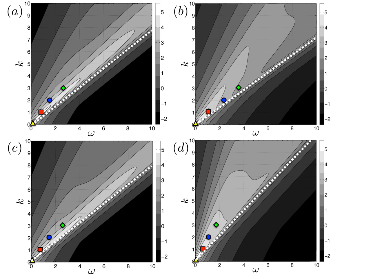
Figure 12: Distribution of amplification $\log_{10}(\sigma_{k,6,\omega,1})$ (a) reference: smooth pipe (b) case I: large drag-decrease $(A^{+},k_{c})=(10,10)$, (c) case II: small drag-decrease $(A^{+},k_{c})=(0.7,10)$, (d) case III: drag-increase $(A^{+},k_{c})=(2,2)$. Symbols denote the frequency corresponding to the most energetic two-dimensional DMD modes with $k=0,1,2,3$ dominant wavenumber. Dashed lines indicate the wavespeed corresponding to the centerline velocity $\bar{u}^{c}(R)$ for each case.

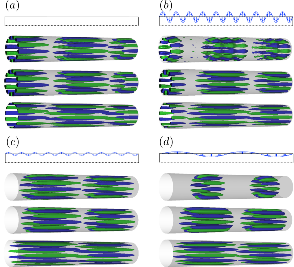
Figure 13: In each of the four blocks, the upper diagram represents each transpiration configuration. Below, iso-surfaces of $50\%$ of the maximum/minimum streamwise velocity are represented corresponding to (top) DMD mode with dominant wavenumbers $k=1$ and $n=6$ (red squares in figure 12) (middle) DMD modes axially-filtered at $k=1$ (bottom) resolvent mode associated with $k=1$ and $n=6$ at the same frequency. (a) reference: smooth pipe (b) case I: large drag-decrease $(A^{+},k_{c})=(10,10)$, (c) case II: small drag-decrease $(A^{+},k_{c})=(0.7,10)$, (d) case III: drag-increase $(A^{+},k_{c})=(2,2)$.

We focus on the effect of transpiration on large scale motions. Hence the broad parameter space $(k,n,\omega)$ is reduced by taking into consideration findings from the literature. As discussed in detail by Sharma & McKeon (2013), VLSMs in pipe flows can be represented with resolvent modes of lengths scales $(k,n)=(1,6)$ and with a convective velocity $c=2/3$ of the centerline streamwise velocity. This representation is based on the work of Monty et al. (2007) and Bailey & Smits (2010), which experimentally investigated the spanwise length scale associated with the VLSM and found to be of the order of the outer length scale, $n=6$. Hence we consider only the azimuthal wavenumber $n=6$.

Reference values of the amplification are provided in contours in Figure 12(a), which show the distribution of resolvent amplification $\log_{10}(\sigma_{k,6,\omega,1})$ for the smooth pipe in a continuum set of $(k,\omega)$ wavenumbers for $n=6$. We observe a narrow band of high amplification caused by a critical-layer mechanism (McKeon & Sharma, 2010). This critical-layer mechanism can be described by examining the resolvent operator. The diagonal terms of the inverse of the resolvent matrix in (38) read

$$h_{ii}=\left[\mathrm{i}(ku_{0}-\omega)u+Re^{-1}\nabla^{2}u\right]^{-1}\,,$$ (48)

thus, for a given value of the Laplacian, there is a large amplification if the wavespeed $c=\omega/k$ matches the mean streamwise velocity, i.e. $c=u_{0}$. That means that flow structures that travel at the local mean velocity create high amplification. Furthermore, we note that straight lines that pass through the origin in figure 12 correspond to constant wavespeed values. The wavespeed corresponding to the centerline velocity is indicated by a dashed line.

Turning first to figure 12(a), the symbols represent the dominant wavenumber and the frequency corresponding to the four most energetic DMD modes at $n=6$. The value of the energy corresponding to each the four modes is similar and omitted. As explained by Gómez et al. (2014), a sparsity is observed in energy as a consequence of the critical layer mechanism in a finite length periodic domain; only structures with an integer axial wavenumber, $k_{i}=1,2,\ldots$ can exist in the flow because of the finite length periodic domain with length $L=4\pi R$. This fact creates a corresponding sparsity in frequency. For each integer axial wavenumber $k_{i}$ there is a frequency $\omega_{i}$ for which the critical layer mechanism occurs, i.e. $\omega_{i}=k_{i}c=k_{i}u_{0}(r_{c})$, with $r_{c}$ being the wall-normal location of the critical layer. This energy sparsity behaviour is clearly observed in the reference case, as shown in figure 12(a), in which the peak frequencies are approximately harmonics. Thus they are approximately aligned in a constant wavespeed line.

We also observe that, for a given $k$, the frequencies corresponding to the peaks of energy differ from the most amplified frequency. As observed by Gómez et al. (2015), this is related to the major role that the non-linear forcing $\chi_{n,\omega,n}$ maintaining the turbulence plays in the resolvent decomposition (42). Nevertheless, we observe that the frequency corresponding to the most energetic modes can be found in the proximity of the high amplification band.

Furthermore, the fact there is only one narrow band of amplification indicates a unique critical layer and that each frequency corresponds to only one wavenumber. This result is confirmed through the similar features exhibited by the most energetically relevant flow structures, arising from DMD of the DNS data, and the resolvent modes associated with the same frequency and wavenumber. For instance, figure 13(a) presents a comparison of the DMD and resolvent mode corresponding to $k=1$ (red square in figure 12(a)). We observe that both DMD and resolvent modes present a unique dominant wavenumber $k=1$ with a similar wall-normal location of its maximum/minimum velocity. The DMD analysis makes use of two-dimensional DNS snapshots based on the Fourier decomposition in (8) and so it permits multiple axial wavenumbers. Hence, the DMD modes are not constrained to one unique dominant axial wavenumber. This does not apply to the resolvent modes, which only admit one wavenumber $k$ by construction of the model. This uniqueness of a dominant streamwise wavenumber in the most energetic flow structures of a smooth pipe flow has also been observed in the work of Gómez et al. (2014). Additionally, figure 13(a) presents DMD modes axially-filtered to $k=1$ to ease comparisons with the resolvent modes. We consider it most appropriate to show the axial velocity because it is the energetically dominant velocity component in these flow structures. Additionally, the flow structures corresponding to positive and negative azimuthal wavenumber $n=\pm 6$ have been summed; a single azimuthal wavenumber necessarily corresponds to a helical shape.

Figure 12(b) represents the amplification results of case I, corresponding to large drag-decrease with $(A^{+},k_{c})=(10,10)$. The effect of transpiration on the flow dynamics is significant; two constant-wavespeed rays of high amplification may be observed. One of the wavespeeds is similar than the one corresponding the critical layer in the reference case while the second one is much faster, almost coincident with the centerline velocity. Also the amplification in the area between these two constant wavespeed lines is increased with respect to the reference case. Hence multiple axial wavenumber $k$ could be amplified at each frequency. This is confirmed in figure 13(b), which shows that the DMD mode features waviness corresponding to multiple wavenumbers. Although the dominant axial wavenumber $k=1$ can be visually identified, other wavenumbers corresponding to interactions of this $k=1$ with the transpiration wavenumber $k_{c}=10$ are also observed. The waviness in figure 13(b) is steady; it does not travel with the $k=1$ flow structure. This has been confirmed via animations of the flow structures and it was expected as a result of the steady transpiration.

As mentioned before, the resolvent modes arise from a one-dimensional model based on a $(k,n,\omega)$ Fourier decomposition hence they only contain one axial wavenumber $k$. As such, a single resolvent mode cannot directly replicate the waviness. However, it provides a description of the dominant wavenumber flow structure. Nevertheless, the axially-filtered DMD mode in figure 13(b) presents a similar structure to the resolvent mode. Similarly to the reference case, the wavespeed based on the dominant wavenumber of the DMD modes are aligned in a constant wavespeed line near the high amplification regions, as seen in 12(b) .

Figure 12(c) shows that the small transpiration $(A^{+},k_{c})=(0.7,10)$ does not have a significant influence on the flow dynamics. The main difference with respect to the reference case is that the amplification line is slightly broader in this case. Consistent with this result, the DMD mode in Figure 13(b) shows a tiny waviness corresponding to other wavenumbers. Similarly to the previous cases, the resolvent mode replicates the dominant axial wavenumber flow structure.

The amplification and energy results corresponding to the drag-increase case $(A^{+},k_{c})=(2,2)$ are shown in Figure 12(d). We observe that, in agreement with the decrease of bulk velocity, the transpiration slows down the flow dynamics; the wavespeed corresponding to the critical layer is slower than in previous cases, i.e., a steeper dashed line in Figure 12(d). Additionally, the critical layer is broad in contrast to the reference case, indicating that multiple axial wavenumbers could be excited. As such, the DMD mode in figure 13(d) shows a dominant axial wavenumber $k=1$ which interacts with others in order to produce two steady localized areas of fluctuating velocity. These clusters are located slightly after the two blowing sections, which corresponding to the high velocity areas in figure 10(d). As in previous cases, the resolvent mode at $k=1$ captures the same dynamics of the filtered DMD mode.

7 Discussion and conclusions

The main features of low- and high-amplitude wall transpiration applied to pipe flow have been investigated by means of direct numerical simulation at Reynolds number $Re_{\tau}=314$. Turbulence statistics have been collected during parameter sweeps of different transpiration amplitudes and wavenumbers. The effect of transpiration is assessed in terms of changes in the bulk axial flow.

We have shown that for low amplitude transpiration the mean streamwise velocity profile follows a velocity defect law, so the outer flow is unaffected by transpiration. This indicates that the flow still obeys Townsend’s similarity hypothesis (Townsend, 1976), as it is usually observed in rough walls. Hence, low amplitude transpiration has a similar effect as roughness or corrugation in a pipe. On the other hand, high amplitude transpiration has a dramatic effect on the outer layer of the velocity profile and the overlap region is substituted by a large increase in streamwise velocity.

We have observed that a transpiration configuration with a small transpiration wavenumber leads to long regions of suction in which the streamwise mean velocity is significantly reduced and the fluctuating velocity can be suppressed. In contrast, a large transpiration wavenumber can speed up the outer layer of the streamwise mean profile with respect to the uncontrolled pipe flow, even at small amplitudes.

These trends in amplitude and wavenumber have permitted the identification of transpiration configurations that lead to a significant drag increase or decrease. For instance, we have shown that a wall transpiration that combines a large amplitude with a large wavenumber creates a large increase in flow rate.

A comparison with the channel flow data of Quadrio et al. (2007) revealed that application of low amplitude transpiration to the pipe flow leads to similar quantitative results.

The obtained turbulence statistics showed that the changes in Reynolds stress induced by the transpiration are not sufficient to explain the overall change in the mean profile. An analysis of the streamwise momentum equation revealed three different physical mechanisms that act in the flow: modification of Reynolds shear stress, steady streaming and generation of non-zero mean streamwise gradients. Additionally, a triple decomposition of the velocity based on a mean profile, a two-dimensional deviation from the mean profile and a fluctuating velocity, has been employed to examine the streamwise momentum equation. This decomposition showed that the steady streaming term can be interpreted as a coherent Reynolds stress generated by the deviation velocity. The contribution of this coherent Reynolds stress to the momentum balance is important close to the wall and it affects the viscous sublayer, which is no longer linear under the influence of transpiration.

The behaviour of these terms has been examined by selected transpiration cases of practical interest in terms of drag modification. For all cases considered, the steady streaming terms opposes to the flow rate while the change in Reynolds shear stress are always positive. This concurs with the numerical simulations of Quadrio et al. (2007); Hoepffner & Fukagata (2009) and the perturbation analysis of Woodcock et al. (2012). Additionally, we have observed that the contribution of non-zero mean streamwise gradients is significant. This contribution can be negative for small transpiration wavenumbers; the turbulent fluctuations are suppressed in the large areas of suction, favoring non-homogeneity effects in the axial direction.

A description of the change in the flow dynamics induced by the transpiration has been obtained via the resolvent analysis methodology introduced by McKeon & Sharma (2010). This framework has been extended to deal with pipe flows with an axially-invariant cross-section but with mean spatial periodicity induced by changes in boundary conditions. The extension involves a triple decomposition based on mean, deviation and fluctuating velocities. This new formulation opens up a new avenue for modifying turbulence using only the mean profile and it could be applied to investigate the flow dynamics of pulsatile flows or changes induced by dynamic roughness.

In the present investigation, this input–output analysis showed that the critical-layer mechanism dominates the behaviour of the fluctuating velocity in pipe flow under transpiration. However, axially periodic transpiration actuation acts to delocalize the critical layer by distorting the mean flow, so that multiple wavenumbers can be excited. This produces waviness of the flow structures.

The resolvent results in this case are useful as a tool to interpret the dynamics but are less directly useful to predict the effects of transpiration, since transpiration feeds directly into altering the mean flow, which itself is required as an input to the resolvent analysis. This limitation partly arises owing to the use of steady actuation, since low-amplitude time-varying actuation directly forces inputs to the resolvent rather than altering its structure (see figure 11)

The critical layer mechanism concentrates the response to actuation in the wall-normal location of the critical layer associated with the wavespeed calculated from the frequency and wavenumber of the actuation. This leads us to believe that, within this framework, dynamic actuation may be more useful for directly targeting specific modes in localised regions of the flow.

DMD of the DNS data confirmed that the transpiration mainly provides a waviness to the leading DMD modes. This corrugation of the flow structures is steady and corresponds to interactions of the critical-layer induced wavenumber with the transpiration wavenumber. As such, this waviness is responsible for generating steady streaming and non-zero mean streamwise gradients, which it turns modifies the streamwise momentum balance, hence enhancing or decreasing the drag.

Finally, a performance analysis indicated that all the transpiration configurations considered are energetically inefficient. In the most favorable case, the benefit obtained by the drag reduction induced by the transpiration marginally exceeds the cost of applying transpiration. Nevertheless, this is an open loop active flow control system. A passive roughness-based flow control system able to mimic the effect of transpiration would be of high practical interest. Hence, we remark that experience gained through this investigation serves to extend this methodology towards manipulation of flow structures at higher Reynolds numbers; this is the subject of an ongoing investigation.

Appendix A. Triadic interaction induced by the deviation velocity

Without loss of generality, we write the deviation velocity as a single Fourier mode with $l$ axial wavenumber. Then the triple decomposition reads:

$$\hat{\bm{u}}(x,r,\theta,t)=\underbrace{\bar{\bm{u}}(r)}_{\mbox{A}}+\underbrace{{\bm{u}}_{l}^{\prime}(r)e^{\mathrm{i}lx}}_{\mbox{B}}+\overbrace{\sum_{(k,n,\omega)\neq(l,0,0)}{\bm{u}}_{k,n,\omega}(r)e^{\mathrm{i}(kx+n\theta-\omega t)}}^{\mbox{C}}+\mathrm{c.c.}$$ (49)

As an example, we substitute this decomposition in the nonlinear terms $\hat{u}\partial_{x}\hat{u}$

$$\hat{u}\partial_{x}\hat{u}=A\partial_{x}A+A\partial_{x}B+A\partial_{x}C+B\partial_{x}A+B\partial_{x}B+B\partial_{x}C+C\partial_{x}A+C\partial_{x}B+C\partial_{x}C\,,$$ (50)

since $\partial_{x}A=0$ we obtain

$$\hat{u}\partial_{x}\hat{u}=A\partial_{x}B+A\partial_{x}C+B\partial_{x}B+B\partial_{x}C+C\partial_{x}B+C\partial_{x}C\,.$$ (51)

Next, we study which terms are orthogonal to the complex exponential functions corresponding to $(k,n,\omega)\neq(0,0,0)$ and $(k,n,\omega)\neq(l,0,0)$. Thus

$$\hat{u}\partial_{x}\hat{u}=\cancel{A\partial_{x}B}+\underbrace{A\partial_{x}C}_{\mbox{$k\bar{u}u_{k,n,\omega}$}}+\cancel{B\partial_{x}B}+\overbrace{B\partial_{x}C}^{\mbox{$(k\pm l){u^{\prime}_{l}}u_{k\pm l,n,\omega}$}}+\underbrace{C\partial_{x}B}_{\mbox{$\pm l{u^{\prime}_{l}}u_{k\pm l,n,\omega}$}}+\overbrace{C\partial_{x}C}^{\mbox{$f_{k,n,\omega}$}}\,.$$ (52)

As a consequence of the triadic interaction between the spatial Fourier mode of the deviation velocity and the fluctuating velocity, there is a coupling of the fluctuating velocity at $(k,n,\omega)$ with that at $(k\pm l,n,\omega)$. This interaction generates the new terms $B\partial_{x}C$ and $C\partial_{x}B$. These two terms are represented by the coupling operator $\mathcal{C}_{k,n,\omega}$ in the resolvent formulation (36). Note that the term $A\partial_{x}B$ is included in the deviation equation $(k,n,\omega)=(l,0,0)$ while the term $B\partial_{x}B$ contributes to the mean flow equation $(k,n,\omega)=(0,0,0)$ as coherent Reynolds stress.

References

- del Álamo & Jiménez (2006) del Álamo, J. C. & Jiménez, J. 2006 Linear energy amplification in turbulent channels. J. Fluid Mech. 559, 205–213.
- Bailey & Smits (2010) Bailey, S. C. C. & Smits, A. J. 2010 Experimental investigation of the structure of large-and very-large-scale motions in turbulent pipe flow. J. Fluid Mech. 651, 339–356.
- Blackburn et al. (2013) Blackburn, H. M., Hall, P. & Sherwin, S. J. 2013 Lower branch equilibria in Couette flow: the emergence of canonical states for arbitrary shear flows. J. Fluid Mech. 726, 58–85.
- Blackburn et al. (2007) Blackburn, H. M., Ooi, A. S. H. & Chong, M. S. 2007 The effect of corrugation height on flow in a wavy-walled pipe. In 16th Australasian Fluid Mechanics Conference, pp. 559–574. The University of Queensland, Gold Coast.
- Blackburn & Sherwin (2004) Blackburn, H. M. & Sherwin, S. J. 2004 Formulation of a Galerkin spectral element–Fourier method for three-dimensional incompressible flows in cylindrical geometries. J. Comput. Phys. 197 (2), 759–778.
- Blasius (1913) Blasius, H. 1913 The law of similarity of frictional processes in fluids. (originally in German), Forsch Arbeit Ingenieur-Wesen, Berlin p. 131.
- Chen et al. (2012) Chen, K.K., Tu, J.H. & Rowley, C.W. 2012 Variants of dynamic mode decomposition: boundary condition, Koopman, and Fourier analyses. Journal of Nonlinear Science 22 (6), 887–915.
- Chin et al. (2010) Chin, C., Ooi, A. S. H., Marusic, I. & Blackburn, H. M. 2010 The influence of pipe length on turbulence statistics computed from direct numerical simulation data. J. Fluid Mech. 22 (11), 115107.
- Choi et al. (1994) Choi, H., Moin, P. & Kim, J. 1994 Active turbulence control for drag reduction in wall-bounded flows. J. Fluid Mech. 262, 75–110.
- den Toonder & Nieuwstadt (1997) den Toonder, J. M. J. & Nieuwstadt, F. T. M. 1997 Reynolds number effects in a turbulent pipe flow for low to moderate Re. Phys. Fluids 9 (11), 3398–3409.
- Fukagata et al. (2002) Fukagata, K., Iwamoto, K. & Kasagi, N. 2002 Contribution of Reynolds stress distribution to the skin friction in wall-bounded flows. Phys. Fluids 14 (11), L73–L76.
- Gómez et al. (2014) Gómez, F., Blackburn, H. M., Rudman, M., McKeon, B.J., Luhar, M., Moarref, R. & Sharma, A.S. 2014 On the origin of frequency sparsity in direct numerical simulations of turbulent pipe flow. Phys. Fluids 26 (10), 101703.
- Gómez et al. (2015) Gómez, F., Blackburn, H. M., Rudman, M., McKeon, B.J. & Sharma, A.S. 2015 On the coupling of direct numerical simulation and resolvent analysis. In Progress in Turbulence VI: proceedings of the iTi Conference in Turbulence. Springer.
- Guala et al. (2006) Guala, M., Hommema, S. E. & Adrian, R. J. 2006 Large-scale and very-large-scale motions in turbulent pipe flow. J. Fluid Mech. 554, 521–542.
- Hama (1954) Hama, F. R. 1954 Boundary-layer characteristics for smooth and rough surfaces. Trans. Soc. Naval Archit. Mar. Engnrs. 62, 333–358.
- Hellström & Smits (2014) Hellström, L.H.O. & Smits, A. J. 2014 The energetic motions in turbulent pipe flow. Phys. Fluids 26 (12), 125102.
- Hellström et al. (2011) Hellström, L. H. O., Sinha, A. & Smits, A. J. 2011 Visualizing the very-large-scale motions in turbulent pipe flow. Phys. Fluids 23 (1), 011703.
- Hoepffner & Fukagata (2009) Hoepffner, J. & Fukagata, K. 2009 Pumping or drag reduction? J. Fluid Mech. 635, 171–187.
- Hutchins & Marusic (2007) Hutchins, N. & Marusic, I. 2007 Evidence of very long meandering features in the logarithmic region of turbulent boundary layers. J. Fluid Mech. 579, 1–28.
- Jiménez & Pinelli (1999) Jiménez, J. & Pinelli, A. 1999 The autonomous cycle of near-wall turbulence. J. Fluid Mech. 389, 335–359.
- Jimenez et al. (2001) Jimenez, J., Uhlmann, M., Pinelli, A. & Kawahara, G. 2001 Turbulent shear flow over active and passive porous surfaces. J. Fluid Mech. 442, 89–117.
- Karniadakis et al. (1991) Karniadakis, G. E., Israeli, M. & Orszag, S. A. 1991 High-order splitting methods for the incompressible Navier–Stokes equations. J. Comput. Phys. 97 (2), 414–443.
- Kasagi et al. (2009) Kasagi, N., Hasegawa, Y. & Fukagata, K. 2009 Toward cost-effective control of wall turbulence for skin friction drag reduction. In Advances in turbulence XII, pp. 189–200. Springer.
- Kim (2011) Kim, J. 2011 Physics and control of wall turbulence for drag reduction. Philosophical Transactions of the Royal Society A: Mathematical, Physical and Engineering Sciences 369 (1940), 1396–1411.
- Kim & Bewley (2007) Kim, J. & Bewley, T. R. 2007 A linear systems approach to flow control. Annu. Rev. Fluid Mech. 39 (1), 383—417.
- Kim et al. (1987) Kim, J., Moin, P. & Moser, R. 1987 Turbulence statistics in fully developed channel flow at low Reynolds number. J. Fluid Mech. 177, 133–166.
- Kim & Adrian (1999) Kim, KC & Adrian, RJ 1999 Very large-scale motion in the outer layer. Phys. Fluids 11 (2), 417–422.
- Luchini (2008) Luchini, P. 2008 Acoustic streaming and lower-than-laminar drag in controlled channel flow. In Progress in Industrial Mathematics at ECMI 2006, pp. 169–177. Springer.
- Luhar et al. (2014) Luhar, M., Sharma, A. S. & McKeon, B. J. 2014 Opposition control within the resolvent analysis framework. J. Fluid Mech. 749, 597–626.
- Mao et al. (2015) Mao, X., Blackburn, H. M. & Sherwin, S. J. 2015 Nonlinear optimal suppression of vortex shedding from a circular cylinder. J. Fluid Mech. 775, 241–265.
- Marusic et al. (2007) Marusic, I., Joseph, D. D. & Mahesh, K. 2007 Laminar and turbulent comparisons for channel flow and flow control. J. Fluid Mech. 570, 467–477.
- McKeon & Sharma (2010) McKeon, B. J. & Sharma, A. S. 2010 A critical layer framework for turbulent pipe flow. J. Fluid Mech. 658, 336–382.
- McKeon et al. (2013) McKeon, B. J., Sharma, A. S. & Jacobi, I. 2013 Experimental manipulation of wall turbulence: A systems approach. Phys. Fluids 25 (3), 031301.
- Meseguer & Trefethen (2003) Meseguer, A. & Trefethen, L. N. 2003 Linearized pipe flow to Reynolds number . J. Comput. Phys. 186 (1), 178–197.
- Mezić (2013) Mezić, Igor 2013 Analysis of fluid flows via spectral properties of the Koopman operator. Annual Review of Fluid Mechanics 45, 357–378.
- Min et al. (2006) Min, T., Kang, S. M., Speyer, J. L. & Kim, J. 2006 Sustained sub-laminar drag in a fully developed channel flow. J. Fluid Mech. 558, 309–318.
- Monty et al. (2007) Monty, J. P., Stewart, J. A., Williams, R. C. & Chong, M. S. 2007 Large-scale features in turbulent pipe and channel flows. J. Fluid Mech. 589, 147–156.
- Quadrio (2011) Quadrio, M. 2011 Drag reduction in turbulent boundary layers by in-plane wall motion. Philosophical Transactions of the Royal Society A: Mathematical, Physical and Engineering Sciences 369 (1940), 1428–1442.
- Quadrio et al. (2007) Quadrio, M., Floryan, J. M. & Luchini, P. 2007 Effect of streamwise-periodic wall transpiration on turbulent friction drag. J. Fluid Mech. 576, 425–444.
- Quadrio & Ricco (2004) Quadrio, M. & Ricco, P. 2004 Critical assessment of turbulent drag reduction through spanwise wall oscillations. J. Fluid Mech. 521, 251–271.
- Rowley et al. (2009) Rowley, C. W., Mezić, I., Bagheri, S., Schlatter, P. & Henningson, D. S. 2009 Spectral analysis of nonlinear flows. J. Fluid Mech. 641, 115–127.
- Saha et al. (2011) Saha, S., Chin, C., Blackburn, H. M. & Ooi, A. S. H. 2011 The influence of pipe length on thermal statistics computed from DNS of turbulent heat transfer. Intnl J. Heat Fluid Flow 32 (6), 1083–1097.
- Saha et al. (2015a) Saha, S., Klewicki, J. C., Ooi, A. S. H. & Blackburn, H.M. 2015a Comparison of thermal scaling properties between turbulent pipe and channel flows via DNS. Int. J. Therm. Sci. 89, 43–57.
- Saha et al. (2015b) Saha, S., Klewicki, J. C., Ooi, A. S. H. & Blackburn, H. M. 2015b Scaling properties of pipe flows with sinusoidal transversely-corrugated walls. J. Fluid Mech. 779, 245–274.
- Saha et al. (2014) Saha, S., Klewicki, J. C., Ooi, A. S. H., Blackburn, H. M. & Wei, T. 2014 Scaling properties of the equation for passive scalar transport in wall-bounded turbulent flows. Intnl J. Heat Mass Transfer 70, 779–792.
- Schmid (2007) Schmid, P. J. 2007 Nonmodal stability theory. Annu. Rev. Fluid Mech. 39 (1), 129–162.
- Schmid (2010) Schmid, P. J. 2010 Dynamic mode decomposition of numerical and experimental data. J. Fluid Mech. 656, 5–28.
- Sharma & McKeon (2013) Sharma, A. S. & McKeon, B. J. 2013 On coherent structure in wall turbulence. J. Fluid Mech. 728, 196–238.
- Sharma et al. (2011) Sharma, A. S., Morrison, J. F., McKeon, B. J., Limebeer, D. J. N., Koberg, W. H. & Sherwin, S. J. 2011 Relaminarisation of channel flow with globally stabilising linear feedback control. Phys. Fluids 23 (12), 125105.
- Smits et al. (2011) Smits, A. J., McKeon, B. J. & Marusic, I. 2011 High-Reynolds number wall turbulence. Annu. Rev. Fluid Mech. 43, 353–375.
- Spalart & McLean (2011) Spalart, P. R. & McLean, J. D. 2011 Drag reduction: enticing turbulence, and then an industry. Philosophical Transactions of the Royal Society A: Mathematical, Physical and Engineering Sciences 369 (1940), 1556–1569.
- Sumitani & Kasagi (1995) Sumitani, Y. & Kasagi, N. 1995 Direct numerical simulation of turbulent transport with uniform wall injection and suction. AIAA journal 33 (7), 1220–1228.
- Townsend (1976) Townsend, A. A. 1976 The Structure of Turbulent Shear Flow, 2nd edn. Cambridge, UK: Cambridge Univ Press.
- Woodcock et al. (2012) Woodcock, J.D., Sader, J.E. & Marusic, I. 2012 Induced flow due to blowing and suction flow control: an analysis of transpiration. J. Fluid Mech. 690, 366–398.