EUROPEAN ORGANIZATION FOR NUCLEAR RESEARCH (CERN)

​​​ CERN-EP-2016-141 LHCb-PAPER-2016-012 15 June 2016

Measurements of the S-wave fraction in $B^{0}\rightarrow K^{+}\pi^{-}\mu^{+}\mu^{-}$ decays and the $B^{0}\rightarrow K^{\ast}(892)^{0}\mu^{+}\mu^{-}$ differential branching fraction

The LHCb collaboration

A measurement of the differential branching fraction of the decay ${B^{0}\rightarrow K^{\ast}(892)^{0}\mu^{+}\mu^{-}}$ is presented together with a determination of the S-wave fraction of the $K^{+}\pi^{-}$ system in the decay $B^{0}\rightarrow K^{+}\pi^{-}\mu^{+}\mu^{-}$. The analysis is based on $pp$-collision data corresponding to an integrated luminosity of 3 fb^-1 collected with the LHCb experiment. The measurements are made in bins of the invariant mass squared of the dimuon system, $q^{2}$. Precise theoretical predictions for the differential branching fraction of $B^{0}\rightarrow K^{\ast}(892)^{0}\mu^{+}\mu^{-}$ decays are available for the $q^{2}$ region $1.1<q^{2}<6.0\,{\rm GeV}^{2}/c^{4}$. In this $q^{2}$ region, for the $K^{+}\pi^{-}$ invariant mass range $796<m_{K\pi}<996\,{\rm MeV}/c^{2}$, the S-wave fraction of the $K^{+}\pi^{-}$ system in $B^{0}\rightarrow K^{+}\pi^{-}\mu^{+}\mu^{-}$ decays is found to be

$$F_{\rm S}=0.101\pm 0.017({\rm stat})\pm 0.009({\rm syst}),$$

and the differential branching fraction of $B^{0}\rightarrow K^{\ast}(892)^{0}\mu^{+}\mu^{-}$ decays is determined to be

$${\rm d}\mathcal{B}/{\rm d}q^{2}=(0.342_{\,-0.017}^{\,+0.017}({\rm stat})\pm{0.009}({\rm syst})\pm 0.023({\rm norm}))\times 10^{-7}c^{4}/{\rm GeV}^{2}.$$

The differential branching fraction measurements presented are the most precise to date and are found to be in agreement with Standard Model predictions.

Published in JHEP 11 (2016) 047

© CERN on behalf of the LHCb collaboration, licence CC-BY-4.0.

 

1 Introduction

The decay ${{B}^{0}}\!\rightarrow{{K}^{*0}}{\mu^{+}\mu^{-}}$ proceeds via a ${b}\!\rightarrow{s}\,{\ell^{+}}{\ell^{-}}$ flavour-changing neutral-current transition. In the Standard Model (SM), this transition is forbidden at tree level and must therefore occur via a loop-level process. Extensions to the SM predict new particles that can contribute to the ${b}\!\rightarrow{s}\,{\ell^{+}}{\ell^{-}}$ process and affect the rate and angular distribution of the decay. Recently, global analyses of measurements involving ${b}\!\rightarrow{s}\,{\ell^{+}}{\ell^{-}}$ processes have reported significant deviations from SM predictions [1, 2, 3, 4, 5, 6, 7, 8, 9, 10, 11, 12, 13, 14, 15]. These deviations could be explained either by new particles [3, 4, 10, 11, 14, 15, 16] or by unexpectedly large hadronic effects [17, 13, 9].

In this paper, the symbol ${{K}^{*0}}$ denotes any neutral strange meson in an excited state that decays to a $K^{+}$ and a $\pi^{-}$. For invariant masses of the $K^{+}\pi^{-}$ system in the range considered in this analysis, the ${{K}^{*0}}$ decay products are predominantly found in a P- or S-wave state. The fractional size of the scalar (S-wave) component of the ${{K}^{+}}{{\pi}^{-}}$ system ($F_{\rm S}$) depends on the squared invariant mass of the dimuon system (${q^{2}}$). This dependence is expected to be similar to that of the longitudinal polarisation fraction ($F_{\rm L}$) of the ${K}^{*}(892)^{0}$ meson [18, 19, 20].

The S-wave fraction is predicted to be maximal in the ${q^{2}}$ range $1.0<{q^{2}}<6.0{\mathrm{\,Ge\kern-1.00006ptV^{2}\!/}c^{4}}$ [18, 19, 20]. A previous analysis by the LHCb collaboration set an upper limit of $F_{\rm S}<0.07$ at 68% confidence level for invariant masses of the $K^{+}\pi^{-}$ system in the range $792<m_{K\pi}<992{\mathrm{\,Me\kern-1.00006ptV\!/}c^{2}}$ [21]. The measurement was performed by exploiting the phase shift of the ${K}^{*}(892)^{0}$ Breit–Wigner function around the corresponding pole mass.

In all previous determinations of the differential branching fraction of ${{B}^{0}}\!\rightarrow{K}^{*}(892)^{0}{\mu^{+}\mu^{-}}$ decays [21, 22, 23, 24, 25], the ${K}^{*}(892)^{0}$ was selected by requiring a window of size 80–380${\mathrm{\,Me\kern-1.00006ptV\!/}c^{2}}$ around the known ${K}^{*}(892)^{0}$ mass, but no correction was made for the scalar fraction. This fraction was assumed to be small and was treated as a systematic uncertainty. The measurements of the differential branching fraction of ${{B}^{0}}\!\rightarrow{K}^{*}(892)^{0}{\mu^{+}\mu^{-}}$ decays are included in global analyses of ${b}\!\rightarrow{s}\,{\ell^{+}}{\ell^{-}}$ processes. As these analyses make use of theory predictions which are made purely for the resonant P-wave part of the $K^{+}\pi^{-}$ system, an accurate assessment of the S-wave component in ${{B}^{0}}\!\rightarrow{{K}^{*0}}{\mu^{+}}{\mu^{-}}$ decays is critical.

In this paper, the first measurement of $F_{\rm S}$ in ${{B}^{0}}\!\rightarrow{{K}^{*0}}{\mu^{+}\mu^{-}}$ decays is presented. The measurement is performed through a fit to the kaon helicity angle [21, 26], $\theta_{K}$, and the $m_{K\pi}$ spectrum, in the range $644<m_{K\pi}<1200{\mathrm{\,Me\kern-1.00006ptV\!/}c^{2}}$. Motivated by previous estimates of the S-wave fraction [21, 18, 19, 20], $F_{\rm S}$ is also determined in a narrower window of $796<m_{K\pi}<996{\mathrm{\,Me\kern-1.00006ptV\!/}c^{2}}$. The values of $F_{\rm S}$ are reported in eight bins of ${q^{2}}$ of approximately $2{\mathrm{\,Ge\kern-1.00006ptV^{2}\!/}c^{4}}$ width, and in two larger bins $1.1<{q^{2}}<6.0{\mathrm{\,Ge\kern-1.00006ptV^{2}\!/}c^{4}}$ and $15.0<{q^{2}}<19.0{\mathrm{\,Ge\kern-1.00006ptV^{2}\!/}c^{4}}$. The choice of ${q^{2}}$ bins is identical to that of Ref. [27].

The measurements of $F_{\rm S}$ allow the determination of the differential branching fraction of the ${{{B}^{0}}\!\rightarrow{K}^{*}(892)^{0}{\mu^{+}}{\mu^{-}}}$ decay. The differential branching fraction is determined by normalising the ${{{B}^{0}}\!\rightarrow{K}^{*}(892)^{0}{\mu^{+}}{\mu^{-}}}$ yield in each ${q^{2}}$ bin to the total event yield of the ${{{B}^{0}}\!\rightarrow{{J\mskip-3.0mu/\mskip-2.0mu\psi\mskip 2.0mu}}{{K}^{*0}}}$ control channel, where the $J/\psi\rightarrow\mu^{+}\mu^{-}$ decay mode is used. The measurements are made using a $pp$-collision data sample recorded by the LHCb experiment in Run 1, corresponding to an integrated luminosity of 3$\mbox{\,fb}^{-1}$. These data were collected at centre-of-mass energies of $7$ and $8\mathrm{\,Te\kern-1.00006ptV}$ during 2011 and 2012 respectively. The differential branching fraction measurement is complementary to the angular analysis presented in Ref. [27], and supersedes that of Ref. [21]. The latter analysis was performed on a 1$\mbox{\,fb}^{-1}$ subset of the Run 1 data sample.

This paper is organised as follows. Section 2 describes the angular and $m_{K\pi}$ distributions of ${{B}^{0}}\!\rightarrow{{K}^{*0}}{\mu^{+}}{\mu^{-}}$ decays with the $K^{+}\pi^{-}$ system in a P- or S-wave state. Section 3 describes the LHCb detector and the procedure used to generate simulated data. The reconstruction and selection of ${{{B}^{0}}\!\rightarrow{{K}^{+}}{{\pi}^{-}}{\mu^{+}\mu^{-}}}$ candidates are described in Sec. 4. Section 5 describes the parameterisation of the mass distributions and Sec. 6 describes the determination of $F_{\rm S}$, including the method used to correct for the detection and selection biases. The measurement of the differential branching fraction of ${{B}^{0}}\!\rightarrow{K}^{*}(892)^{0}{\mu^{+}\mu^{-}}$ decays is presented in Sec. 7. The systematic uncertainties affecting the measurements are discussed in Sec. 8. Finally, the conclusions are presented in Sec. 9.

2 The angular distribution and $F_{\rm S}$

The final state of the ${{B}^{0}}\!\rightarrow{{K}^{*0}}{\mu^{+}}{\mu^{-}}$ decay is completely described by ${q^{2}}$, and the three decay angles, $\vec{\Omega}\equiv(\cos{\theta_{K}},\,\cos{\theta_{\ell}},\,\phi)$ [21]. The angle between the $\mu^{+}$ ($\mu^{-}$) and the direction opposite to that of the ${{B}^{0}}$ (${{\kern 1.79993pt\overline{\kern-1.79993ptB}{}}{}^{0}}$) meson in the rest frame of the dimuon system is denoted by $\theta_{\ell}$. The angle between the direction of the $K^{+}$ ($K^{-}$) and the ${{B}^{0}}$ (${{\kern 1.79993pt\overline{\kern-1.79993ptB}{}}{}^{0}}$) meson in the rest frame of the ${{K}^{*0}}$ (${{\kern 1.99997pt\overline{\kern-1.99997ptK}{}}{}^{*0}}$) is denoted by $\theta_{K}$. The angle between the plane defined by the dimuon pair and the plane defined by the kaon and pion in the ${{B}^{0}}$ (${{\kern 1.79993pt\overline{\kern-1.79993ptB}{}}{}^{0}}$) rest frame is denoted by $\phi$.

In the limit that the dimuon mass is large compared to the mass of the muons (${q^{2}}\gg 4m_{\mu}^{2}$), this choice of the angular basis allows the differential decay rates of ${{B}^{0}}\!\rightarrow{{K}^{*0}}{\mu^{+}\mu^{-}}$ and ${{\kern 1.79993pt\overline{\kern-1.79993ptB}{}}{}^{0}}\!\rightarrow{{\kern 1.99997pt\overline{\kern-1.99997ptK}{}}{}^{*0}}{\mu^{+}\mu^{-}}$ decays to be written as

$$\begin{split}\!\!\!\!\!\!\!\frac{\mathrm{d}^{5}(\Gamma+\overline{\Gamma})}{\mathrm{d}m_{K\pi}\mathrm{d}{q^{2}}\,\mathrm{d}\vec{\Omega}}=\frac{9}{32\pi}\left[\frac{}{}\right.&\!\!\!\!\left.\frac{}{}{(I_{1}^{s}+\bar{I}_{1}^{s})}\sin^{2}\theta_{K}(1+3\cos 2\theta_{\ell})+{(I_{1}^{c}+\bar{I}_{1}^{c})}\cos^{2}\theta_{K}(1-\cos 2\theta_{\ell})~{}+\right.\\ &\!\!\!\!\left.\frac{}{}{(I_{3}+\bar{I}_{3})}\sin^{2}\theta_{K}\sin^{2}\theta_{\ell}\cos 2\phi+{{(I_{4}+\bar{I}_{4})\sin 2\theta_{K}\sin 2\theta_{\ell}\cos\phi}}~{}+\right.\\ &\!\!\!\!\frac{}{}\left.{{{(I_{5}+\bar{I}_{5})}\sin 2\theta_{K}\sin\theta_{\ell}\cos\phi}}+(I_{6s}+\bar{I}_{6s})\sin^{2}\theta_{K}\cos\theta_{\ell}~{}+\right.\\ &\!\!\!\!\frac{}{}\left.{{{(I_{7}+\bar{I}_{7})}\sin 2\theta_{K}\sin\theta_{\ell}\sin\phi}}+{{{(I_{8}+\bar{I}_{8})}\sin 2\theta_{K}\sin 2\theta_{\ell}\sin\phi}}~{}+\right.\\ &\!\!\!\!\frac{}{}\left.(I_{9}+\bar{I}_{9})\sin^{2}\theta_{K}\sin^{2}\theta_{\ell}\sin 2\phi+(I_{10}+\bar{I}_{10})(1-\cos 2\theta_{\ell})~{}+\right.\\ &\!\!\!\!\frac{}{}\left.(I_{11}+\bar{I}_{11})\cos\theta_{K}(1-\cos 2\theta_{\ell})~{}+\right.\\ &\!\!\!\!\frac{}{}\left.(I_{14}+\bar{I}_{14})\sin\theta_{K}\sin 2\theta_{\ell}\cos\phi+(I_{15}+\bar{I}_{15})\sin\theta_{K}\sin\theta_{\ell}\cos\phi~{}+\right.\\ &\!\!\!\!\frac{}{}\left.(I_{16}+\bar{I}_{16})\sin\theta_{K}\sin\theta_{\ell}\sin\phi+(I_{17}+\bar{I}_{17})\sin\theta_{K}\sin 2\theta_{\ell}\sin\phi\frac{}{}\right],\\ \end{split}$$ (1)

where $\Gamma$ and $\overline{\Gamma}$ denote the decay rates of the ${{B}^{0}}$ and ${{\kern 1.79993pt\overline{\kern-1.79993ptB}{}}{}^{0}}$ respectively. The 15 coefficients $I_{j}$ ($\bar{I}_{j}$) are bilinear combinations of the ${{K}^{*0}}$ (${{\kern 1.99997pt\overline{\kern-1.99997ptK}{}}{}^{*0}}$) decay amplitudes and vary with ${q^{2}}$ and $m_{K\pi}$. The numbering of the coefficients follows the convention used in Ref. [27]. Coefficients $I_{j}$ with $j\leq 9$ involve P-wave amplitudes only, coefficient $I_{10}$ involves S-wave amplitudes only and coefficients with $11\leq j\leq 17$ describe the interference between P- and S-wave amplitudes [28].

The polarity of the LHCb dipole magnet, discussed in Sec. 3, is reversed periodically. Coupled with the fact that ${{B}^{0}}$ and ${{\kern 1.79993pt\overline{\kern-1.79993ptB}{}}{}^{0}}$ decays are studied simultaneously, this results in a symmetric detection efficiency in $\phi$. Therefore, the angular distribution is simplified by performing a transformation of the $\phi$ angle such that

$$\phi^{\prime}=\begin{cases}\phi+\pi&\text{~{}if~{}}\phi<0\\ \phi&\text{~{}otherwise},\end{cases}$$ (2)

which results in the cancellation of terms in Eq. 1 that have a $\sin\phi$ or $\cos\phi$ dependence.

The remaining $I_{j}$ and $\bar{I}_{j}$ coefficients can be written in terms of the decay amplitudes given in Ref. [27]. Defining $\vec{\Omega}^{\prime}\equiv(\cos{\theta_{K}},\,\cos{\theta_{\ell}},\,\phi^{\prime})$, the resulting differential decay rate has the form

$$\begin{split}\frac{\mathrm{d}^{5}(\Gamma+\overline{\Gamma})}{\mathrm{d}m_{K\pi}\mathrm{d}{q^{2}}\,\mathrm{d}\vec{\Omega}^{\prime}}=&\,\frac{1}{4\pi}G_{\rm S}\left|f_{\rm LASS}(m_{K\pi})\right|^{2}(1-\cos{2\theta_{\ell}})~{}+\\ &\frac{3}{4\pi}G_{\rm P}^{0}\left|f_{\rm BW}(m_{K\pi})\right|^{2}\cos^{2}\theta_{K}(1-\cos{2\theta_{\ell}})~{}+\\ &\frac{\sqrt{3}}{2\pi}{\rm Re}\left[\left(G_{\rm SP}^{\rm Re}+iG_{\rm SP}^{\rm Im}\right)f_{\rm LASS}(m_{K\pi})f^{\ast}_{\rm BW}(m_{K\pi})\right]\cos{\theta_{K}}(1-\cos{2\theta_{\ell}})+~{}\\ &\frac{9}{16\pi}G_{\rm P}^{\perp\parallel}\left|f_{\rm BW}(m_{K\pi})\right|^{2}\sin^{2}\theta_{K}\left(1+\frac{1}{3}\cos{2\theta_{\ell}}\right)+~{}\\ &\frac{3}{8\pi}S_{3}(G_{\rm P}^{0}+G_{\rm P}^{\perp\parallel})\left|f_{\rm BW}(m_{K\pi})\right|^{2}\sin^{2}\theta_{K}\sin^{2}\theta_{\ell}\cos{2\phi^{\prime}}+~{}\\ &\frac{3}{2\pi}A_{\rm FB}(G_{\rm P}^{0}+G_{\rm P}^{\perp\parallel})\left|f_{\rm BW}(m_{K\pi})\right|^{2}\sin^{2}\theta_{K}\cos{\theta_{\ell}}+~{}\\ &\frac{3}{4\pi}S_{9}(G_{\rm P}^{0}+G_{\rm P}^{\perp\parallel})\left|f_{\rm BW}(m_{K\pi})\right|^{2}\sin^{2}\theta_{K}\sin^{2}\theta_{\ell}\sin{2\phi^{\prime}},\end{split}$$ (3)

where $f_{\rm BW}(m_{K\pi})$ denotes the $m_{K\pi}$ dependence of the resonant P-wave component, which is modelled using a relativistic Breit–Wigner function. The S-wave component is modelled using the LASS parameterisation [29], $f_{\rm LASS}(m_{K\pi})$. The exact definitions of the P- and S-wave line shapes are given in Appendix A. The real-valued coefficients $G_{\rm S}^{\phantom{R}}$, $G_{\rm SP}^{\rm Re}$, $G_{\rm SP}^{\rm Im}$, $G_{\rm P}^{0}$ and $G_{\rm P}^{\perp\parallel}$ are bilinear combinations of the $q^{2}$-dependent parts of the ${{K}^{*0}}$ (${{\kern 1.99997pt\overline{\kern-1.99997ptK}{}}{}^{*0}}$) helicity amplitudes $A_{i}^{L,R}({q^{2}})$ ($\overline{A}_{i}^{L,R}({q^{2}})$) and are given by

$$G_{\rm S}^{\phantom{R}}= \,|A_{S}^{L}({q^{2}})|^{2}+|A_{S}^{R}({q^{2}})|^{2}+|\overline{A}_{S}^{L}({q^{2}})|^{2}+|\overline{A}_{S}^{R}({q^{2}})|^{2},$$

$$G_{\rm SP}^{\rm Re}+iG_{\rm SP}^{\rm Im}= \,A_{S}^{L}A_{0}^{L\ast}+A_{S}^{R}A_{0}^{R\ast}+\overline{A}_{S}^{L}\overline{A}_{0}^{L\ast}+\overline{A}_{S}^{R}\overline{A}_{0}^{R\ast},$$

$$G_{\rm P}^{0}= \,|A_{0}^{L}({q^{2}})|^{2}+|A_{0}^{R}({q^{2}})|^{2}+|\overline{A}_{0}^{L}({q^{2}})|^{2}+|\overline{A}_{0}^{R}({q^{2}})|^{2},$$ (4)

$$G_{\rm P}^{\perp\parallel}= \displaystyle\sum\limits_{i=\perp,\parallel}|A_{i}^{L}({q^{2}})|^{2}+|A_{i}^{R}({q^{2}})|^{2}+|\overline{A}_{i}^{L}({q^{2}})|^{2}+|\overline{A}_{i}^{R}({q^{2}})|^{2},$$

where $L$ and $R$ denote the (left- and right-handed) chiralities of the dimuon system. These coefficients are determined through the extended maximum likelihood fit described in Sec. 6.2. The coefficients $S_{3}$, $A_{\rm FB}$ and $S_{9}$ are $C\!P$-averaged observables that are defined in Ref. [27]. The integral of Eq. 3 with respect to $\cos{\theta_{\ell}}$ and $\phi^{\prime}$ is independent of these observables. However, detection effects that are either asymmetric or non-uniform in $\cos{\theta_{\ell}}$ and $\phi^{\prime}$ introduce a residual dependence on these observables. In this analysis, $S_{3}$, $A_{\rm FB}$ and $S_{9}$ are set to their measured values [27]. The systematic uncertainty associated with this choice is negligible.

Using the definitions of Eq. 2, the S-wave fraction $F_{\rm S}$ in the range $a<m_{K\pi}<b$ can be determined from the coefficients $G_{\rm S}^{\phantom{R}}$ and $G_{\rm P}^{0,\perp\parallel}$, through

$$F_{\rm S}|_{a}^{b}=\frac{G_{\rm S}^{\phantom{R}}\int_{a}^{b}{\textrm{d}m_{K\pi}\left|f_{\rm LASS}(m_{K\pi})\right|^{2}}}{G_{\rm S}\int_{a}^{b}\textrm{d}m_{K\pi}\left|f_{\rm LASS}(m_{K\pi})\right|^{2}+\left(G_{\rm P}^{0}+G_{\rm P}^{\perp\parallel}\right)\int_{a}^{b}\textrm{d}m_{K\pi}\left|f_{\rm BW}(m_{K\pi})\right|^{2}}.$$ (5)

3 Detector and simulation

The LHCb detector [30, 31] is a single-arm forward spectrometer covering the pseudorapidity range $2<\eta<5$, designed for the study of particles containing $b$ or $c$ quarks. The detector includes a high-precision tracking system divided into three sub-systems: a silicon-strip vertex detector surrounding the $pp$ interaction region, a large-area silicon-strip detector that is located upstream of a dipole magnet with a bending power of about $4{\mathrm{\,Tm}}$, and three stations of silicon-strip detectors and straw drift tubes situated downstream of the magnet. The tracking system provides a measurement of the momentum, $p$, of charged particles with a relative uncertainty that varies from 0.5% at low momentum to 1.0% at 200${\mathrm{\,Ge\kern-1.00006ptV\!/}c}$. The minimum distance of a track to a primary vertex (PV), the impact parameter, is measured with a resolution of $(15+29/\mbox{$p_{\mathrm{T}}$}){\,\upmu\mathrm{m}}$, where $p_{\mathrm{T}}$ is the component of the momentum transverse to the beam, in ${\mathrm{\,Ge\kern-1.00006ptV\!/}c}$. Different types of charged hadrons are distinguished using information from two ring-imaging Cherenkov (RICH) detectors. Photons, electrons and hadrons are identified by a calorimeter system consisting of scintillating-pad and preshower detectors, an electromagnetic calorimeter and a hadronic calorimeter. Muons are identified by a system composed of alternating layers of iron and multiwire proportional chambers. The online event selection is performed by a trigger [32], which consists of a hardware stage, based on information from the calorimeter and muon systems, followed by a software stage, which applies a full event reconstruction.

A large sample of simulated events is used to determine the effect of the detector geometry, trigger, and the selection criteria on the angular distribution of the signal, and to determine the ratio of efficiencies between the signal and the ${{{B}^{0}}\!\rightarrow{{J\mskip-3.0mu/\mskip-2.0mu\psi\mskip 2.0mu}}{{K}^{*0}}}$ normalisation mode. In the simulation, $pp$ collisions are generated using Pythia [33, *Sjostrand:2007gs] with a specific LHCb configuration [35]. The decay of the ${B}^{0}$ meson is described by EvtGen [36], which generates final-state radiation using Photos [37]. As described in Ref. [38], the Geant4 toolkit [39, *Agostinelli:2002hh] is used to implement the interaction of the generated particles with the detector and the detector response. Data-driven corrections are applied to the simulation following the procedure of Ref. [27]. These corrections account for the small level of mismodelling of the detector occupancy, the ${{B}^{0}}$ momentum and vertex quality, and the particle identification (PID) performance.

4 Selection of signal candidates

The ${{B}^{0}}\!\rightarrow{{K}^{*0}}{\mu^{+}\mu^{-}}$ signal candidates are first required to pass the hardware trigger, which selects events containing at least one muon with transverse momentum $\mbox{$p_{\mathrm{T}}$}>1.48{\mathrm{\,Ge\kern-1.00006ptV\!/}c}$ in the 7$\mathrm{\,Te\kern-1.00006ptV}$ data or $\mbox{$p_{\mathrm{T}}$}>1.76{\mathrm{\,Ge\kern-1.00006ptV\!/}c}$ in the 8$\mathrm{\,Te\kern-1.00006ptV}$ data. In the subsequent software trigger, at least one of the final-state particles is required to have $\mbox{$p_{\mathrm{T}}$}>1.7{\mathrm{\,Ge\kern-1.00006ptV\!/}c}$ in the 7$\mathrm{\,Te\kern-1.00006ptV}$ data or $\mbox{$p_{\mathrm{T}}$}>1.6{\mathrm{\,Ge\kern-1.00006ptV\!/}c}$ in the 8$\mathrm{\,Te\kern-1.00006ptV}$ data, unless the particle is identified as a muon in which case $\mbox{$p_{\mathrm{T}}$}>1.0{\mathrm{\,Ge\kern-1.00006ptV\!/}c}$ is required. The final-state particles that satisfy these transverse momentum criteria are also required to have an impact parameter larger than $100{\,\upmu\mathrm{m}}$ with respect to all PVs in the event. Finally, the tracks of two or more of the final-state particles are required to form a vertex that is significantly displaced from the PVs.

Signal candidates are formed from a pair of oppositely charged tracks that are identified as muons, combined with a ${{K}^{*0}}$ meson candidate. The ${{K}^{*0}}$ candidate is formed from two oppositely charged tracks that are identified as a kaon and a pion. These signal candidates are required to pass a set of loose preselection requirements, which are identical to those described in Ref. [27], with the exception that the ${{K}^{*0}}$ candidate is required to have an invariant mass in the wider $644<m_{K\pi}<1200{\mathrm{\,Me\kern-1.00006ptV\!/}c^{2}}$ range. The preselection requirements exploit the decay topology of ${{B}^{0}}\!\rightarrow{{K}^{*0}}{\mu^{+}}{\mu^{-}}$ transitions and restrict the data sample to candidates with good quality vertex and track fits. Candidates are required to have a reconstructed ${{B}^{0}}$ invariant mass ($m_{K\pi\mu\mu}$) in the range $5170<m_{K\pi\mu\mu}<5780{\mathrm{\,Me\kern-1.00006ptV\!/}c^{2}}$.

The backgrounds formed by combining particles from different $b$- and $c$-hadron decays are referred to as combinatorial. Such backgrounds are suppressed with the use of a Boosted Decision Tree (BDT) [41, 42]. The BDT used for the present analysis is identical to that described in Ref. [27] and the same working point is used. The BDT selection has a signal efficiency of 90% while removing 95% of the combinatorial background surviving the preselection. The efficiency of the BDT is uniform with respect to $m_{K\pi\mu\mu}$ in the above mass range.

Specific background processes can mimic the signal if their final states are misidentified or misreconstructed. The requirements of Ref. [27] are reassessed and found to reduce the sum of all backgrounds from such decay processes to a level of less than 2% of the expected signal yield. The only requirement that is modified in the present analysis is that responsible for removing genuine ${{B}^{0}}\!\rightarrow{{K}^{*0}}{\mu^{+}}{\mu^{-}}$ decays, where the track of the genuine pion is reconstructed with the kaon hypothesis and vice versa. These misidentified signal candidates occur more often in the wider $m_{K\pi}$ window used for the present analysis, and are reduced by tightening the requirements made on the kaon and pion PID information provided by the RICH detectors. After the application of all the selection criteria, this specific background process is reduced to less than 1% of the level of the signal.

5 The $K^{+}\pi^{-}\mu^{+}\mu^{-}$ and $K^{+}\pi^{-}$ mass distributions

The $K^{+}\pi^{-}\mu^{+}\mu^{-}$ invariant mass is used to discriminate between signal and background. The distribution of the signal candidates is modelled using the sum of two Gaussian functions with a common mean, each with a power law tail on the lower side. The parameters describing this model are determined from fits to ${{B}^{0}}\!\rightarrow{{J\mskip-3.0mu/\mskip-2.0mu\psi\mskip 2.0mu}}{{K}^{*0}}$ data in a ${q^{2}}$ range $9.22<{q^{2}}<9.96{\mathrm{\,Ge\kern-1.00006ptV^{2}\!/}c^{4}}$ and with an $m_{K\pi}$ range of $644<m_{K\pi}<1200{\mathrm{\,Me\kern-1.00006ptV\!/}c^{2}}$, shown in Fig. 1. These parameters are fixed for the subsequent fits to the ${{B}^{0}}\!\rightarrow{{K}^{*0}}{\mu^{+}}{\mu^{-}}$ candidates in the same $m_{K\pi}$ range. In samples of simulated ${{B}^{0}}\!\rightarrow{{K}^{*0}}{\mu^{+}}{\mu^{-}}$ decays, the $m_{K\pi\mu\mu}$ resolution is observed to differ from that in ${{B}^{0}}\!\rightarrow{{J\mskip-3.0mu/\mskip-2.0mu\psi\mskip 2.0mu}}{{K}^{*0}}$ decays by 2 to 8% depending on ${q^{2}}$. A correction factor is therefore derived from the simulation and is applied to the widths of the Gaussian functions in the different ${q^{2}}$ bins. In the fits to ${{B}^{0}}\!\rightarrow{{J\mskip-3.0mu/\mskip-2.0mu\psi\mskip 2.0mu}}{{K}^{*0}}$ decays, an additional component is included to account for the ${{{\kern 1.79993pt\overline{\kern-1.79993ptB}{}}{}^{0}_{s}}\!\rightarrow{{J\mskip-3.0mu/\mskip-2.0mu\psi\mskip 2.0mu}}{{K}^{*0}}}$ process. The size of this additional component is taken to be 0.8% of the ${{B}^{0}}\!\rightarrow{{J\mskip-3.0mu/\mskip-2.0mu\psi\mskip 2.0mu}}{{K}^{*0}}$ signal [43]. The fit to the ${{B}^{0}}\!\rightarrow{{J\mskip-3.0mu/\mskip-2.0mu\psi\mskip 2.0mu}}{{K}^{*0}}$ mode gives $389\,577\pm 649$ decays. In the fits to ${{B}^{0}}\!\rightarrow{{K}^{*0}}{\mu^{+}}{\mu^{-}}$ decays, the ${{{\kern 1.79993pt\overline{\kern-1.79993ptB}{}}{}^{0}_{s}}\!\rightarrow{{K}^{*0}}{\mu^{+}\mu^{-}}}$ contribution is neglected. The systematic uncertainty related to ignoring this background process is negligible. For both ${{B}^{0}}\!\rightarrow{{J\mskip-3.0mu/\mskip-2.0mu\psi\mskip 2.0mu}}{{K}^{*0}}$ and ${{B}^{0}}\!\rightarrow{{K}^{*0}}{\mu^{+}}{\mu^{-}}$ decays, the combinatorial background in the $K^{+}\pi^{-}\mu^{+}\mu^{-}$ invariant mass spectrum is described by an exponential function. The ${{B}^{0}}\!\rightarrow{{K}^{*0}}{\mu^{+}}{\mu^{-}}$ yield integrated over the ${q^{2}}$ ranges $0.1<{q^{2}}<8.0{\mathrm{\,Ge\kern-1.00006ptV^{2}\!/}c^{4}}$, $11.0<{q^{2}}<12.5{\mathrm{\,Ge\kern-1.00006ptV^{2}\!/}c^{4}}$ and $15.0<{q^{2}}<19.0{\mathrm{\,Ge\kern-1.00006ptV^{2}\!/}c^{4}}$ is determined to be $2593\pm 60$. The ${q^{2}}$ regions $8.0<{q^{2}}<11.0{\mathrm{\,Ge\kern-1.00006ptV^{2}\!/}c^{4}}$ and $12.5<{q^{2}}<15.0{\mathrm{\,Ge\kern-1.00006ptV^{2}\!/}c^{4}}$ are dominated by the contributions from ${{B}^{0}}\!\rightarrow{{J\mskip-3.0mu/\mskip-2.0mu\psi\mskip 2.0mu}}{{K}^{*0}}$ and ${{{B}^{0}}\!\rightarrow{\psi{(2S)}}{{K}^{*0}}}$ decays respectively and are therefore excluded in the fits to the signal ${{B}^{0}}\!\rightarrow{{K}^{*0}}{\mu^{+}}{\mu^{-}}$ decays.

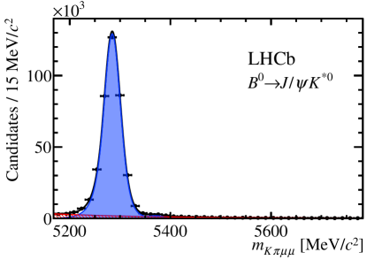
Figure 1: Invariant mass $m_{K\pi\mu\mu}$ of (left) the ${{B}^{0}}\!\rightarrow{{J\mskip-3.0mu/\mskip-2.0mu\psi\mskip 2.0mu}}{{K}^{*0}}$ decay and (right) the signal decay ${{B}^{0}}\!\rightarrow{{K}^{*0}}{\mu^{+}}{\mu^{-}}$ integrated over the ${q^{2}}$ regions described in the text. The individual signal (blue shaded area) and background (red hatched area) components are shown. The solid line denotes the total fitted distribution.

As discussed in Sec. 2, the $K^{+}\pi^{-}$ invariant mass distribution of the signal candidates is modelled with two distributions. A relativistic Breit–Wigner function is used for the P-wave component and the LASS parameterisation for the S-wave component. The parameters of these functions are fixed to the values determined in ${{B}^{0}}\!\rightarrow{{J\mskip-3.0mu/\mskip-2.0mu\psi\mskip 2.0mu}}{{K}^{*0}}$ decays using the model described in Ref. [44]. A systematic uncertainty is assigned for this choice.

The $K^{+}\pi^{-}$ invariant mass distribution of the combinatorial background is modelled using an empirical threshold function of the form

$$f_{\rm bkg}(m_{K\pi})=(m_{K\pi}-m_{\rm thr})^{1/\alpha},$$ (6)

where $m_{\rm thr}=634{\mathrm{\,Me\kern-1.00006ptV\!/}c^{2}}$ is given by the sum of the pion and kaon masses [45], and $\alpha$ is a parameter determined from fits to the data. This model has been validated on data from the upper $m_{K\pi\mu\mu}$ sideband, defined as $5350<m_{K\pi\mu\mu}<5780{\mathrm{\,Me\kern-1.00006ptV\!/}c^{2}}$, where no resonant structure in the $m_{K\pi}$ spectrum is observed.

6 Determination of the S-wave fraction

6.1 Efficiency correction

The trigger, selection, and detector geometry bias the distributions of the decay angles $\cos{\theta_{K}}$, $\cos{\theta_{\ell}}$, $\phi^{\prime}$, as well as the ${q^{2}}$ and $m_{K\pi}$ distributions. The dominant sources of bias are the geometrical acceptance of the detector and the requirements on the track momentum, the impact parameter, and the PID of the hadrons.

The method for obtaining the efficiency correction, described in Ref [27], is extended to also include the $m_{K\pi}$ dimension. The detection efficiency is expressed in terms of orthonormal Legendre polynomials of order $n$, $P_{n}(x)$, as

$$\epsilon({q^{2}},m_{K\pi},\vec{\Omega}^{\prime})=\sum\limits_{g,h,i,j,k}c_{ghijk}P_{g}(m_{K\pi})P_{h}(\cos{\theta_{\ell}})P_{i}(\cos{\theta_{K}})P_{j}(\phi^{\prime})P_{k}({{q^{2}}}).$$ (7)

As the polynomials are orthonormal over the domain $x\in[-1,1]$, the observables $m_{K\pi}$, $\phi^{\prime}$, and ${q^{2}}$ are linearly transformed to lie within this domain when evaluating the efficiency. The sum in Eq. 7 runs up to 5^th order for $\cos{\theta_{K}}$ and $\phi^{\prime}$, and up to 8^th, 7^th and 6^th order for $\cos{\theta_{\ell}}$, ${q^{2}}$ and $m_{K\pi}$ respectively. The coefficients $c_{ghijk}$ are determined using a principal moment analysis of simulated four-body ${{{B}^{0}}\!\rightarrow{{K}^{+}}{{\pi}^{-}}{\mu^{+}\mu^{-}}}$ phase-space decays. Two-dimensional projections of the detection efficiency as a function of $\cos{\theta_{K}}$–${q^{2}}$ and $m_{K\pi}$–${q^{2}}$ are shown in Fig. 2.

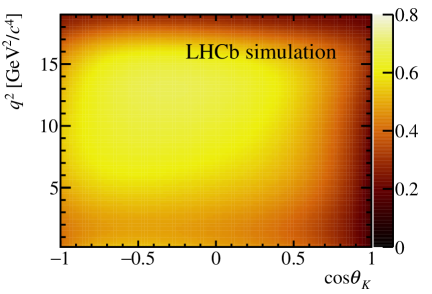
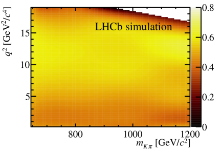
Figure 2: Two-dimensional projections of the efficiency (left) in the $\cos{\theta_{K}}$–${q^{2}}$ plane and (right) in the $m_{K\pi}$–${q^{2}}$ plane, determined from a principal moments analysis of simulated four-body ${{{B}^{0}}\!\rightarrow{{K}^{+}}{{\pi}^{-}}{\mu^{+}\mu^{-}}}$ phase-space decays. The colour scale denotes the efficiency in arbitrary units. The lack of entries in the top right corner of the $m_{K\pi}$–${q^{2}}$ distribution is due to the limited phase space available in the decay of the ${{B}^{0}}$ meson.

6.2 Fit to the mass and angular distributions

An extended maximum likelihood fit to $m_{K\pi\mu\mu}$, $m_{K\pi}$ and $\cos{\theta_{K}}$ is performed in each bin of ${q^{2}}$ in order to determine the coefficients $G_{\rm S}^{\phantom{R}}$, $G_{\rm SP}^{\rm Re}$, $G_{\rm SP}^{\rm Im}$ and $G_{\rm P}^{\perp\parallel}$ averaged over the ${q^{2}}$ bin. Given these coefficients, the S-wave fraction $F_{\rm S}$ is extracted using Eq. 5. The angular distribution of the signal is described by Eq. 3 multiplied by the efficiency model evaluated at the centre of the ${q^{2}}$ bin ($q^{2}_{\rm bc}$). Integrating over $\cos{\theta_{\ell}}$ and $\phi^{\prime}$ simplifies the fit, while retaining the sensitivity to the parameters related to $F_{\rm S}$. The resulting angular and $m_{K\pi}$ distribution of the signal, $P_{\rm sig}$, within a bin $q^{2}_{\rm min}<{q^{2}}<q^{2}_{\rm max}$, is given by

$$P_{\rm sig}(m_{K\pi},\cos{\theta_{K}})=\int_{q^{2}_{\rm min}}^{q^{2}_{\rm max}}\int_{0}^{\pi}\int_{-1}^{1}\mathrm{d}\!\cos{\theta_{\ell}}{\rm d}\phi^{\prime}\textrm{d}{q^{2}}\left[\frac{\mathrm{d}^{5}(\Gamma+\overline{\Gamma})}{\mathrm{d}m_{K\pi}\mathrm{d}{q^{2}}\,\mathrm{d}\vec{\Omega}^{\prime}}\times\epsilon(q^{2}_{\rm bc},m_{K\pi},\vec{\Omega}^{\prime})\right],$$ (8)

The overall scale of $P_{\rm sig}$ is set by fixing the parameter $G_{\rm P}^{0}$ to an arbitrary value. The $m_{K\pi\mu\mu}$ distribution of the signal is assumed to factorise with $P_{\rm sig}(m_{K\pi},\cos{\theta_{K}})$. This assumption is validated using simulated events.

The $\cos{\theta_{K}}$ distribution of the combinatorial background is modelled with a second-order polynomial where all parameters are allowed to vary in the fit. The $m_{K\pi}$, $m_{K\pi\mu\mu}$ and $\cos{\theta_{K}}$ distributions of the combinatorial background are assumed to factorise. This assumption has been validated on data from the upper $m_{K\pi\mu\mu}$ sideband. Figure 3 shows the projections of the probability distribution function on the angular and mass distributions for the ${q^{2}}$ bin $1.1<{q^{2}}<6.0{\mathrm{\,Ge\kern-1.00006ptV^{2}\!/}c^{4}}$. Projections of other ${q^{2}}$ bins are provided in Appendix B.

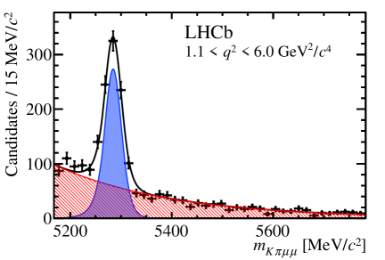
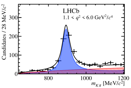
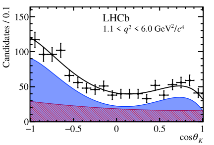
Figure 3: Angular and mass distributions for the ${q^{2}}$ bin $1.1<{q^{2}}<6.0{\mathrm{\,Ge\kern-1.00006ptV^{2}\!/}c^{4}}$. The distributions of $\cos{\theta_{K}}$ and $m_{K\pi}$ are shown for candidates in the signal $m_{K\pi\mu\mu}$ window of $\pm 50{\mathrm{\,Me\kern-1.00006ptV\!/}c^{2}}$ around the known ${{B}^{0}}$ mass. The solid line denotes the total fitted distribution. The individual components, signal (blue shaded area) and background (red hatched area), are also shown.

6.3 Result for $F_{\rm S}$

Using Eq. 5, $F_{\rm S}$ is determined in the full $m_{K\pi}$ region of the fit, $\left.F_{\rm S}\right|_{644}^{1200}$, and in the narrow $m_{K\pi}$ region, $\left.F_{\rm S}\right|_{796}^{996}$. The statistical uncertainty on $F_{\rm S}$ is determined using the following procedure. Values of the parameters of the fit are generated according to a multi-dimensional bifurcated Gaussian distribution. This distribution is constructed out of the correlation matrix of the fit and the asymmetric uncertainties obtained from a profile likelihood. For each generated set of parameters of the fit, a value of $F_{\rm S}$ is computed. The 68% confidence interval is defined by taking the $16^{\rm th}$–$84^{\rm th}$ percentiles of the resulting distribution of $F_{\rm S}$. The correct coverage of this method is validated using pseudoexperiments generated with a wide range of $F_{\rm S}$ values.

Figure 4 shows the values of $\left.F_{\rm S}\right|_{644}^{1200}$ and $\left.F_{\rm S}\right|_{796}^{996}$ in each ${q^{2}}$ bin. The uncertainties given are a quadratic sum of statistical and systematic uncertainties. The results are also reported in Table 1. The sources of systematic uncertainty are detailed in Sec. 8. As expected, the shape of the measured $F_{\rm S}$ distribution is found to be compatible with the smoothly varying distribution of $F_{\rm L}$ measured in Ref. [27].

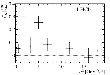
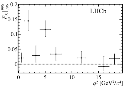
Figure 4: Results for the S-wave fraction ($F_{\rm S}$) in bins of $q^{2}$ in the range (left) $644<m_{K\pi}<1200{\mathrm{\,Me\kern-1.00006ptV\!/}c^{2}}$ and (right) $796<m_{K\pi}<996{\mathrm{\,Me\kern-1.00006ptV\!/}c^{2}}$. The uncertainties shown are the quadratic sum of the statistical and systematic uncertainties. The shape of $F_{\rm S}$ is found to be compatible with the smoothly varying distribution of $F_{\rm L}$, as measured in Ref. [27].

Table 1: S-wave fraction ($F_{\rm S}$) in bins of ${q^{2}}$ for two $m_{K\pi}$ regions. The first uncertainty is statistical and the second systematic.

$q^{2}$ bin $(\!{\mathrm{\,Ge\kern-1.00006ptV^{2}\!/}c^{4}})$	$\left.F_{\rm S}\right|_{796}^{996}$	$\left.F_{\rm S}\right|_{644}^{1200}$
$0.10<{q^{2}}<0.98$	$\phantom{+}0.021_{\,-0.011}^{\,+0.015}\pm{0.009}$	$\phantom{+}0.052_{\,-0.027}^{\,+0.035}\pm{0.013}$
$1.1<{q^{2}}<2.5$	$\phantom{+}0.144_{\,-0.030}^{\,+0.035}\pm{0.010}$	$\phantom{+}0.304_{\,-0.053}^{\,+0.058}\pm{0.013}$
$2.5<{q^{2}}<4.0$	$\phantom{+}0.029_{\,-0.020}^{\,+0.031}\pm{0.010}$	$\phantom{+}0.071_{\,-0.049}^{\,+0.069}\pm{0.015}$
$4.0<{q^{2}}<6.0$	$\phantom{+}0.117_{\,-0.023}^{\,+0.027}\pm{0.008}$	$\phantom{+}0.254_{\,-0.044}^{\,+0.048}\pm{0.012}$
$6.0<{q^{2}}<8.0$	$\phantom{+}0.033_{\,-0.019}^{\,+0.022}\pm{0.009}$	$\phantom{+}0.082_{\,-0.045}^{\,+0.049}\pm{0.016}$
$11.0<{q^{2}}<12.5$	$\phantom{+}0.021_{\,-0.016}^{\,+0.021}\pm{0.007}$	$\phantom{+}0.049_{\,-0.039}^{\,+0.048}\pm{0.014}$
$15.0<{q^{2}}<17.0$	$-0.008_{\,-0.014}^{\,+0.033}\pm{0.006}$	$-0.016_{\,-0.030}^{\,+0.069}\pm{0.012}$
$17.0<{q^{2}}<19.0$	$\phantom{+}0.018_{\,-0.017}^{\,+0.013}\pm{0.009}$	$\phantom{+}0.034_{\,-0.032}^{\,+0.024}\pm{0.019}$
$1.1<{q^{2}}<6.0$	$\phantom{+}0.101_{\,-0.017}^{\,+0.017}\pm{0.009}$	$\phantom{+}0.224_{\,-0.033}^{\,+0.032}\pm{0.013}$
$15.0<{q^{2}}<19.0$	$\phantom{+}0.010_{\,-0.014}^{\,+0.017}\pm{0.007}$	$\phantom{+}0.019_{\,-0.025}^{\,+0.030}\pm{0.015}$

The presence of a nonresonant P-wave component in the $K^{+}\pi^{-}$ system has been suggested in Refs. [46, 47]. However, no evidence for such a component was found in the current data sample. The effect of neglecting a nonresonant P-wave contribution with a relative phase and magnitude varied within the statistical uncertainties determined in this analysis, was found to be negligible.

7 Differential branching fraction of the decay ${{{B}^{0}}\!\rightarrow{K}^{*}(892)^{0}{\mu^{+}}{\mu^{-}}}$

The differential branching fraction of the decay ${{{B}^{0}}\!\rightarrow{K}^{*}(892)^{0}{\mu^{+}}{\mu^{-}}}$ is estimated by normalising the signal yield, $n_{{{K}^{*0}}\mu^{+}\mu^{-}}$, obtained from the fit described in Sec. 6.2, to the total event yield of the decay ${{{B}^{0}}\!\rightarrow{{J\mskip-3.0mu/\mskip-2.0mu\psi\mskip 2.0mu}}{{K}^{*0}}}$, $n_{{{J\mskip-3.0mu/\mskip-2.0mu\psi\mskip 2.0mu}}{{K}^{*0}}}$. The number of ${{{B}^{0}}\!\rightarrow{{J\mskip-3.0mu/\mskip-2.0mu\psi\mskip 2.0mu}}{{K}^{*0}}}$ events is obtained from a fit to the $m_{K\pi\mu\mu}$ spectrum using the same ${q^{2}}$ range as for the fit to determine the $m_{K\pi\mu\mu}$ mass shape parameters (Sec. 5), but for an $m_{K\pi}$ range $796<m_{K\pi}<996~{}{\mathrm{\,Me\kern-1.00006ptV\!/}c^{2}}$. This yield has to be corrected for the S-wave fraction within the narrow $m_{K\pi}$ window of ${{{B}^{0}}\!\rightarrow{{J\mskip-3.0mu/\mskip-2.0mu\psi\mskip 2.0mu}}{{K}^{*0}}}$ decays, $F_{\rm S}^{{{J\mskip-3.0mu/\mskip-2.0mu\psi\mskip 2.0mu}}{{K}^{*0}}}$. The value of $F_{\rm S}^{{{J\mskip-3.0mu/\mskip-2.0mu\psi\mskip 2.0mu}}{{K}^{*0}}}$ is obtained from Ref. [48] and is adjusted to the $m_{K\pi}$ range $796<m_{K\pi}<996~{}{\mathrm{\,Me\kern-1.00006ptV\!/}c^{2}}$. The ratio of ${{B}^{0}}\!\rightarrow{{K}^{*0}}{\mu^{+}}{\mu^{-}}$ and ${{{B}^{0}}\!\rightarrow{{J\mskip-3.0mu/\mskip-2.0mu\psi\mskip 2.0mu}}{{K}^{*0}}}$ events is corrected for the relative efficiency between the two decays, $R_{\epsilon}=\epsilon_{J/\psi{{K}^{*0}}}/\epsilon_{{{K}^{*0}}\mu^{+}\mu^{-}}$. This ratio is determined using simulated samples of ${{{B}^{0}}\!\rightarrow{K}^{*}(892)^{0}{\mu^{+}}{\mu^{-}}}$ and ${{{B}^{0}}\!\rightarrow{{J\mskip-3.0mu/\mskip-2.0mu\psi\mskip 2.0mu}}{K}^{*}(892)^{0}}$ decays. The angular distributions of these samples are corrected to account for the presence of P- and S-wave components with a relative abundance given by the measurements of Sec. 6.3 and Ref. [48]. The systematic uncertainty associated with this correction is determined by varying the components within the uncertainties of the measured values and recalculating $R_{\epsilon}$. The resulting uncertainty on $R_{\epsilon}$ is negligible.

The differential branching fraction of ${{{B}^{0}}\!\rightarrow{K}^{*}(892)^{0}{\mu^{+}}{\mu^{-}}}$ decays in a ${q^{2}}$ bin of width $(q^{2}_{\rm max}-q^{2}_{\rm min})$ is given by

$$\begin{split}\frac{\textrm{d}\mathcal{B}}{\textrm{d}{q^{2}}}=&\frac{R_{\epsilon}}{(q^{2}_{\rm max}-q^{2}_{\rm min})}\frac{(1-\left.F_{\rm S}\right|_{644}^{1200})n_{{{K}^{*0}}\mu^{+}\mu^{-}}}{(1-F_{\rm S}^{{{J\mskip-3.0mu/\mskip-2.0mu\psi\mskip 2.0mu}}{{K}^{*0}}})n_{{{J\mskip-3.0mu/\mskip-2.0mu\psi\mskip 2.0mu}}{{K}^{*0}}}}\mathcal{B}({{{B}^{0}}\!\rightarrow{{J\mskip-3.0mu/\mskip-2.0mu\psi\mskip 2.0mu}}{{K}^{*0}}})\mathcal{B}({{J\mskip-3.0mu/\mskip-2.0mu\psi\mskip 2.0mu}}\rightarrow\mu^{+}\mu^{-}),\end{split}$$ (9)

where $\left.F_{\rm S}\right|_{644}^{1200}$, $R_{\epsilon}$ and $n_{{{K}^{*0}}\mu^{+}\mu^{-}}$ correspond to quantities measured within the relevant ${q^{2}}$ bin. The branching fraction $\mathcal{B}({{B}^{0}}\rightarrow{{J\mskip-3.0mu/\mskip-2.0mu\psi\mskip 2.0mu}}{K}^{*}(892)^{0})$ obtained from Ref. [49] is

$$\mathcal{B}({{B}^{0}}\rightarrow{{J\mskip-3.0mu/\mskip-2.0mu\psi\mskip 2.0mu}}{K}^{*}(892)^{0})=(1.19\pm 0.01\pm 0.08)\times 10^{-3},$$

where the first uncertainty is statistical and the second systematic. The branching fraction for ${{J\mskip-3.0mu/\mskip-2.0mu\psi\mskip 2.0mu}}\rightarrow\mu^{+}\mu^{-}$ decays is taken from Ref. [45]. The resulting differential branching fraction is shown in Fig. 5. The uncertainties given are a quadratic sum of statistical and systematic uncertainties and the bands shown indicate the SM prediction from Refs. [50, 51]. The results are also reported in Table 2. The various sources of systematic uncertainties are described in Sec. 8.

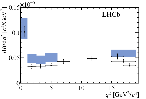
Figure 5: Differential branching fraction of ${{{B}^{0}}\!\rightarrow{K}^{*}(892)^{0}{\mu^{+}}{\mu^{-}}}$ decays as a function of ${q^{2}}$. The data are overlaid with the SM prediction from Refs. [50, 51]. No SM prediction is included in the region close to the narrow $c\bar{c}$ resonances. The result in the wider $q^{2}$ bin $15.0<{q^{2}}<19.0{\mathrm{\,Ge\kern-1.00006ptV^{2}\!/}c^{4}}$ is also presented. The uncertainties shown are the quadratic sum of the statistical and systematic uncertainties, and include the uncertainty on the ${{{B}^{0}}\!\rightarrow{{J\mskip-3.0mu/\mskip-2.0mu\psi\mskip 2.0mu}}{{K}^{*0}}}$ and ${{J\mskip-3.0mu/\mskip-2.0mu\psi\mskip 2.0mu}}\rightarrow\mu^{+}\mu^{-}$ branching fractions.

Table 2: Differential branching fraction of ${{{B}^{0}}\!\rightarrow{K}^{*}(892)^{0}{\mu^{+}}{\mu^{-}}}$ decays in bins of ${q^{2}}$. The first uncertainty is statistical, the second systematic and the third due to the uncertainty on the ${{{B}^{0}}\!\rightarrow{{J\mskip-3.0mu/\mskip-2.0mu\psi\mskip 2.0mu}}{{K}^{*0}}}$ and ${{J\mskip-3.0mu/\mskip-2.0mu\psi\mskip 2.0mu}}\rightarrow\mu^{+}\mu^{-}$ branching fractions.

$q^{2}$ bin $(\!{\mathrm{\,Ge\kern-1.00006ptV^{2}\!/}c^{4}})$	$\textrm{d}\mathcal{B}/\textrm{d}{q^{2}}\times 10^{-7}$ $(c^{4}/\mathrm{\,Ge\kern-1.00006ptV}^{2})$
$0.10<{q^{2}}<0.98$	$1.016_{\,-0.073}^{\,+0.067}\pm{0.029}\pm 0.069$
$1.1<{q^{2}}<2.5$	$0.326_{\,-0.031}^{\,+0.032}\pm{0.010}\pm 0.022$
$2.5<{q^{2}}<4.0$	$0.334_{\,-0.033}^{\,+0.031}\pm{0.009}\pm 0.023$
$4.0<{q^{2}}<6.0$	$0.354_{\,-0.026}^{\,+0.027}\pm{0.009}\pm 0.024$
$6.0<{q^{2}}<8.0$	$0.429_{\,-0.027}^{\,+0.028}\pm{0.010}\pm 0.029$
$11.0<{q^{2}}<12.5$	$0.487_{\,-0.032}^{\,+0.031}\pm{0.012}\pm 0.033$
$15.0<{q^{2}}<17.0$	$0.534_{\,-0.037}^{\,+0.027}\pm{0.020}\pm 0.036$
$17.0<{q^{2}}<19.0$	$0.355_{\,-0.022}^{\,+0.027}\pm{0.017}\pm 0.024$
$1.1<{q^{2}}<6.0$	$0.342_{\,-0.017}^{\,+0.017}\pm{0.009}\pm 0.023$
$15.0<{q^{2}}<19.0$	$0.436_{\,-0.019}^{\,+0.018}\pm{0.007}\pm 0.030$

The total branching fraction of the ${{{B}^{0}}\!\rightarrow{K}^{*}(892)^{0}{\mu^{+}}{\mu^{-}}}$ decay is obtained from the sum over the eight ${q^{2}}$ bins. To account for the fraction of signal events in the vetoed ${q^{2}}$ regions, a correction factor of $1.532\pm 0.001({\rm stat})\pm 0.010({\rm syst})$ is applied. This factor is determined using the calculation in Ref. [52] and form factors from Ref. [53]. The systematic uncertainty is determined by recalculating the extrapolation factor using the form factors from Ref. [54] and taking the difference to the nominal value. The resulting total branching fraction is

$$\mathcal{B}({{{B}^{0}}\!\rightarrow{K}^{*}(892)^{0}{\mu^{+}}{\mu^{-}}})=(0.904^{\,+0.016}_{\,-0.015}\pm 0.010\pm 0.006\pm 0.061)\times 10^{-6},$$

where the uncertainties, from left to right, are statistical, systematic, from the extrapolation to the full ${q^{2}}$ region and due to the uncertainty of the branching fraction of the normalisation mode.

8 Systematic uncertainties

The sources of systematic uncertainty considered can alter the angular and mass distributions, as well as the ratio of efficiencies between the signal and control channels. In general, the systematic uncertainties are significantly smaller than the statistical uncertainties. The various sources of systematic uncertainty are discussed in detail below and are summarised in Table 3. Motivated by Eq. 9, the systematic uncertainty for $F_{\rm S}$ is presented for the $m_{K\pi}$ region $644<m_{K\pi}<1200{\mathrm{\,Me\kern-1.00006ptV\!/}c^{2}}$. Typical ranges are quoted in order to summarise the effect the systematic uncertainties have across the various ${q^{2}}$ bins. Sources of systematic uncertainty that can affect both $F_{\rm S}$ and the differential branching fraction are treated as 100% correlated.

Table 3: Summary of the main sources of systematic uncertainty on $\left.F_{\rm S}\right|_{644}^{1200}$ and $\textrm{d}\mathcal{B}/\textrm{d}{q^{2}}$. Typical ranges are quoted in order to summarise the effect the systematic uncertainties have across the various ${q^{2}}$ bins.

Source	$\left.F_{\rm S}\right|_{644}^{1200}$	$\textrm{d}\mathcal{B}/\textrm{d}{q^{2}}$ $\times 10^{-7}(c^{4}/\rm{GeV}^{2})$
Data-simulation differences	$0.008$–$0.013$	$0.004$–$0.021$
Efficiency model	$0.001$–$0.010$	$0.001$–$0.012$
S-wave $m_{K\pi}$ model	$0.001$–$0.017$	$0.001$–$0.015$
${{B}^{0}}\rightarrow{K}^{*}(892)^{0}$ form factors	–	$0.003$–$0.017$
$\mathcal{B}({{B}^{0}}\!\rightarrow{{J\mskip-3.0mu/\mskip-2.0mu\psi\mskip 2.0mu}}(\rightarrow\mu^{+}\mu^{-}){{K}^{*0}})$	–	$0.025$–$0.079$

8.1 Systematic uncertainties on the S-wave fraction

The impact of each source of systematic uncertainty on $F_{\rm S}$ is estimated using pseudoexperiments, where samples are generated varying one or more parameters. The value of $F_{\rm S}$ is determined using both the nominal model and the alternative model. For every pseudoexperiment, the difference between the two values of $F_{\rm S}$ is computed. In general, the systematic uncertainty is then taken as the average of this difference over a large number of pseudoexperiments. The exception to this is the statistical uncertainty of the efficiency correction. In order to account for this statistical variation, the standard deviation of the difference between the two values of $F_{\rm S}$ from each pseudoexperiment is used instead. The systematic uncertainty is evaluated in each ${q^{2}}$ bin separately. The pseudodata are generated with signal and background yields many times larger than those of the data, rendering statistical effects negligible. The main systematic uncertainties on $F_{\rm S}$ originate from the efficiency correction function and the choice of model used to describe the S-wave component of the $m_{K\pi}$ distribution of the signal.

There are two main systematic uncertainties associated with the efficiency correction function used for determining $F_{\rm S}$. Firstly, an uncertainty arises from residual data-simulation differences. After all corrections to the simulation are applied, a difference at the level of 10% remains in the momentum spectrum of the pions between simulated and genuine ${{B}^{0}}\!\rightarrow{{J\mskip-3.0mu/\mskip-2.0mu\psi\mskip 2.0mu}}{{K}^{*0}}$ decays. A new efficiency correction is derived after weighting the simulated phase-space sample to account for this difference. The second main systematic uncertainty associated with the efficiency correction is due to the order of the polynomials used to describe the efficiency function. To evaluate this uncertainty, a new efficiency correction is derived in which the polynomial order in $q^{2}$ is increased by two. This change is motivated by a small residual difference between the ${q^{2}}$ dependence of the nominal efficiency correction and the simulated phase-space sample, near the upper kinematic edge of the ${q^{2}}$ range. Uncertainties due to the limited size of the simulation sample used to derive the efficiency correction, as well as due to the evaluation of the efficiency correction at the centre of the ${q^{2}}$ bin are also assessed and are found to be negligible.

To assess the modelling of the S-wave component in the $m_{K\pi}$ distribution, pseudoexperiments are produced where the LASS line shape is exchanged for the sum of resonant $K^{*}_{0}(800)^{0}$ (also known as the $\kappa$ resonance) and $K^{*}_{0}(1430)^{0}$ contributions. An additional variation is considered where the parameters of the LASS distribution, determined in $B^{0}\rightarrow{{J\mskip-3.0mu/\mskip-2.0mu\psi\mskip 2.0mu}}{{K}^{*0}}$ decays using the model described in Ref. [44], are exchanged for those measured by the LASS collaboration [29]. The largest of the two variations is taken as the systematic uncertainty on the S-wave model. Systematic uncertainties associated with the modelling of the P-wave $m_{K\pi}$ distribution of the signal are found to be negligible.

Integrating the differential decay rate given in Eq. 3 over $\cos{\theta_{\ell}}$ and $\phi^{\prime}$ results in the cancellation of terms involving the angular observables $S_{3}$, $A_{\rm FB}$ and $S_{9}$. However the integral of the product of the differential decay rate with the efficiency correction, given in Eq. 8, results in a residual dependence of the signal distribution on these angular observables. By generating pseudoexperiments with observables $S_{3}$, $A_{\rm FB}$ and $S_{9}$ either set to zero or varied within the uncertainties measured in Ref. [27], the systematic uncertainty on $F_{\rm S}$ is assessed. Even considering the largest variation observed, the resulting systematic uncertainty is negligible.

All other sources of systematic uncertainties described in Ref. [27], such as the modelling of the $m_{K\pi\mu\mu}$ distribution of the signal and background, the choice of the $m_{K\pi}$ and $\cos\theta_{K}$ background models and the effect of residual specific backgrounds, are found to be sub-dominant. The effect of neglecting a possible D-wave $K^{+}\pi^{-}$ component, arising from the tail of the $K^{*}_{2}(1430)^{0}$, is also assessed and found to be negligible.

8.2 Systematic uncertainties on the differential branching fraction

Systematic uncertainties affecting the differential branching fraction predominantly arise through: the knowledge of $R_{\epsilon}$, the ratio of the reconstruction and selection efficiencies described in Sec. 7; the uncertainty of the branching fraction of the decay ${{B}^{0}}\!\rightarrow{{J\mskip-3.0mu/\mskip-2.0mu\psi\mskip 2.0mu}}{{K}^{*0}}$, which is shown as a separate systematic uncertainty in Table 2; and systematic uncertainties related to the determination of $F_{\rm S}$, which are propagated to the differential branching fraction measurement.

The imperfect knowledge of the $B\rightarrow K^{*}$ form-factor model used in the generation of the ${{B}^{0}}\!\rightarrow{{K}^{*0}}{\mu^{+}}{\mu^{-}}$ simulated sample affects the determination of the ratio of efficiencies $R_{\epsilon}$. A systematic uncertainty is therefore assessed by weighting simulated events to account for the variations between the models described in Refs. [50] and [54].

As described in Sec. 8.1, after all corrections to the simulation are applied, a small difference remains in the momentum spectrum of the pions between simulated and genuine ${{B}^{0}}\!\rightarrow{{J\mskip-3.0mu/\mskip-2.0mu\psi\mskip 2.0mu}}{{K}^{*0}}$ decays. The ratio $R_{\epsilon}$, and consequently $\textrm{d}\mathcal{B}/\textrm{d}{q^{2}}$, is therefore calculated by weighting the simulated ${{{B}^{0}}\!\rightarrow{K}^{*}(892)^{0}{\mu^{+}}{\mu^{-}}}$ and ${{{B}^{0}}\!\rightarrow{{J\mskip-3.0mu/\mskip-2.0mu\psi\mskip 2.0mu}}{K}^{*}(892)^{0}}$ decays to account for the observed differences.

Other sources of systematic uncertainties affecting the determination of the signal yield, such as the choice of model to describe the $m_{K\pi\mu\mu}$ distribution of the signal and the background components, the choice of the $m_{K\pi}$ and $\cos\theta_{K}$ models to describe the background, and the effect of residual specific backgrounds, are found to be negligible.

9 Conclusions

This paper presents the first measurement of the S-wave fraction in the $K^{+}\pi^{-}$ system of ${{B}^{0}}\!\rightarrow{{K}^{*0}}{\mu^{+}}{\mu^{-}}$ decays using a data sample corresponding to an integrated luminosity of $3\mbox{\,fb}^{-1}$ collected at the LHCb experiment. Accounting for the measured S-wave fraction in the wide $m_{K\pi}$ region, the first measurement of the P-wave component of the differential branching fraction of ${{{B}^{0}}\!\rightarrow{K}^{*}(892)^{0}{\mu^{+}}{\mu^{-}}}$ decays is reported in bins of ${q^{2}}$. All previous measurements of the differential branching fraction have compared the combination of S- and P-wave components to the theory prediction, which is made purely for the resonant P-wave part of the $K^{+}\pi^{-}$ system. The measurements of the S-wave fraction presented in this paper are compatible with theory predictions [18, 19, 20] and support previous estimates [21]. In the absence of any previous measurement, such estimates have been used to assign a systematic uncertainty for a possible S-wave component [21]. The measurements of the S-wave fraction presented in this paper allow these estimates to be replaced with an accurate assessment of the scalar component in ${{B}^{0}}\!\rightarrow{{K}^{*0}}{\mu^{+}}{\mu^{-}}$ decays. The resulting measurements of the differential branching fraction of ${{{B}^{0}}\!\rightarrow{K}^{*}(892)^{0}{\mu^{+}}{\mu^{-}}}$ decays are the most precise to date and are in good agreement with the SM predictions.

Appendix A The $m_{K\pi}$ distribution of the signal

The $K^{+}\pi^{-}$ invariant mass distribution of the signal candidates is modelled by two distributions. For the P-wave component, a relativistic Breit-Wigner function is used, given by

$$\begin{split}f_{\rm BW}(m_{K\pi})=&\sqrt{kp}\left(\frac{k}{k_{892}}\right)\frac{B^{\prime}_{1}(k,k_{892},d)B^{\prime}_{0}(p,p_{892},d)}{m_{K\pi}^{2}-m_{892}^{2}-im_{892}\Gamma_{892}(m_{K\pi})},\end{split}$$ (10)

where $\sqrt{kp}$ is the phase-space factor, $\Gamma_{892}(m_{K\pi})$ is given by

$$\Gamma_{892}(m_{K\pi})=\Gamma_{892}B^{\prime\,2}_{1}(k,k_{892},d)\left(\frac{k}{k_{892}}\right)^{3}\left(\frac{m_{892}}{m_{K\pi}}\right),$$ (11)

and $B^{\prime}$ are Blatt–Weisskopf barrier factors as defined in Ref. [45]. The parameter $d$ is the meson radius parameter and is set to 1.6$\mathrm{\,Ge\kern-1.00006ptV}^{-1}c$ [44]. The systematic uncertainty associated with the choice of this value is negligible. The parameters $m_{892}$ and $\Gamma_{892}$ are the pole mass and width of the ${K}^{*}(892)^{0}$ resonance, and $k$ ($p$) is the momentum of the $K^{+}$ (${{K}^{*0}}$) in the rest frame of the ${{K}^{*0}}$ (${{B}^{0}}$) evaluated at a given $m_{K\pi}$. The parameters $k_{892}$ and $p_{892}$ are the values of $k$ and $p$ evaluated at the pole mass of the ${K}^{*}(892)^{0}$ resonance. In Eq. 10, the orbital angular momentum between the ${K}^{*}(892)^{0}$ and the dimuon system is considered to be zero. The inclusion of a higher orbital angular momentum component has a negligible effect on the measurements.

The S-wave component of the signal is modelled using the LASS parameterisation [29], given by

$$f_{\rm LASS}(m_{K\pi})=\sqrt{kp}B^{\prime}_{1}(k,k_{1430},d)\left(\frac{k}{k_{1430}}\right)\left(\frac{1}{\cot{\delta_{B}}-i}+e^{2i\delta_{B}}\frac{1}{\cot{\delta_{R}}-i}\right),$$ (12)

where $k_{1430}$ is the momentum of the ${{K}^{*0}}$ in the ${{B}^{0}}$ rest frame, evaluated at the pole mass of the ${K}_{0}^{*}(1430)^{0}$ resonance. The terms $\cot{\delta_{B}}$ and $\cot{\delta_{R}}$ are given by

$$\cot{\delta_{B}}=\frac{1}{ak}+\frac{rk}{2}$$ (13)

and

$$\cot{\delta_{R}}=\frac{m_{1430}^{2}-m_{K\pi}^{2}}{m_{1430}\Gamma_{1430}(m_{K\pi})},$$ (14)

with the running width $\Gamma_{1430}(m_{K\pi})$ in turn given by

$$\Gamma_{1430}(m_{K\pi})=\Gamma_{1430}\frac{k}{k_{1430}}\frac{m_{1430}}{m_{K\pi}}\,.$$ (15)

The parameters $m_{1430}$ and $\Gamma_{1430}$ are the pole mass and width of the ${K}_{0}^{*}(1430)^{0}$ resonance, and $k_{1430}$ is the momentum of the kaon in the ${{K}^{*0}}$ rest frame, evaluated at the pole mass of the ${K}_{0}^{*}(1430)^{0}$ resonance. The second term of Eq. 12 is equivalent to a Breit–Wigner function for the ${K}_{0}^{*}(1430)^{0}$. The first term of Eq. 12 contains two empirical parameters $\left\{a,r\right\}$. These parameters are fixed to the values $a=3.83\,{\mathrm{\,Ge\kern-1.00006ptV\!/}c}^{-1}$ and $r=2.86{\mathrm{\,Ge\kern-1.00006ptV\!/}c}^{-1}$, determined in ${{B}^{0}}\!\rightarrow{{J\mskip-3.0mu/\mskip-2.0mu\psi\mskip 2.0mu}}{{K}^{*0}}$ decays using the model described in Ref. [44].

In order to assess the systematic effect of this choice, these parameters are also fixed to values from the LASS experiment, $a=1.94{\mathrm{\,Ge\kern-1.00006ptV\!/}c}^{-1}$ and $r=1.76{\mathrm{\,Ge\kern-1.00006ptV\!/}c}^{-1}$. The resulting systematic uncertainty is found to be negligible.

Appendix B Likelihood fit projections

Figures 6–9 show the projections of the fitted probability density function on $m_{K\pi\mu\mu}$, $m_{K\pi}$ and $\cos{\theta_{K}}$. Figure 6 shows the wider ${q^{2}}$ bins of $1.1<{q^{2}}<6.0{\mathrm{\,Ge\kern-1.00006ptV^{2}\!/}c^{4}}$ and $15.0<{q^{2}}<19.0{\mathrm{\,Ge\kern-1.00006ptV^{2}\!/}c^{4}}$, Figs. 7–9 show the $m_{K\pi\mu\mu}$, $m_{K\pi}$ and $\cos{\theta_{K}}$ projections respectively for the finer ${q^{2}}$ bins. In all figures, the solid line denotes the total fitted distribution. The individual components, signal (blue shaded area) and background (red hatched area), are also shown.

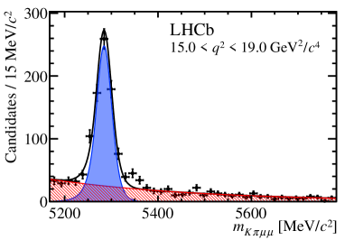
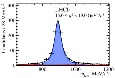
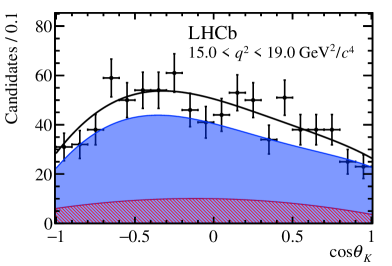
Figure 6: Angular and mass distributions for the ${q^{2}}$ bins $1.1<{q^{2}}<6.0{\mathrm{\,Ge\kern-1.00006ptV^{2}\!/}c^{4}}$ (left) and $15.0<{q^{2}}<19.0{\mathrm{\,Ge\kern-1.00006ptV^{2}\!/}c^{4}}$ (right). The distributions of $\cos{\theta_{K}}$ and $m_{K\pi}$ are shown for candidates in the signal $m_{K\pi\mu\mu}$ window of $\pm 50{\mathrm{\,Me\kern-1.00006ptV\!/}c^{2}}$ around the known ${{B}^{0}}$ mass.

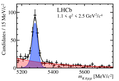
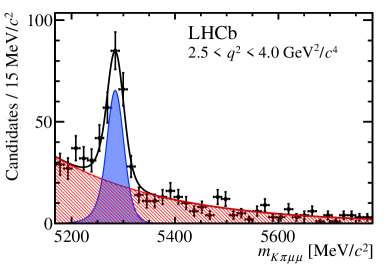
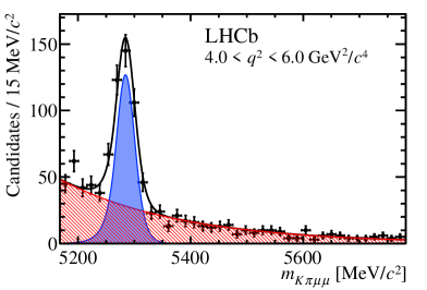
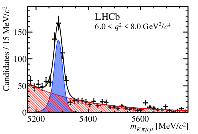
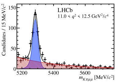
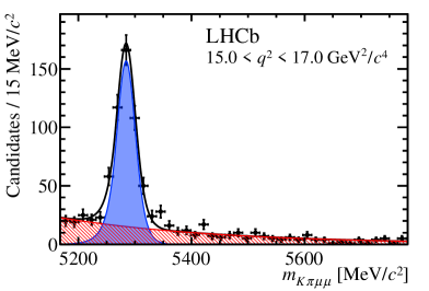
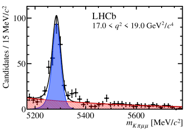
Figure 7: The $K^{+}\pi^{-}\mu^{+}\mu^{-}$ invariant mass distributions for the fine ${q^{2}}$ bins.

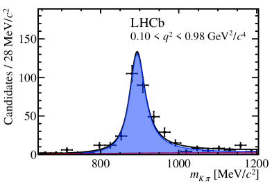
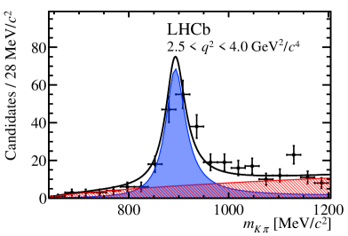
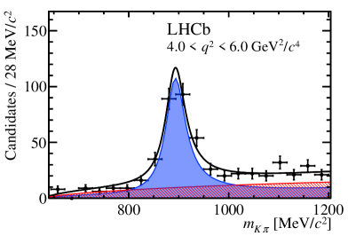
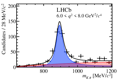
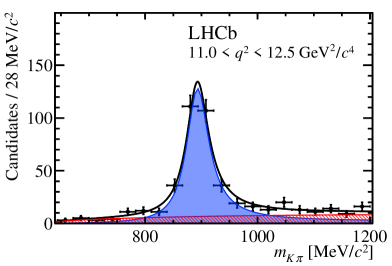
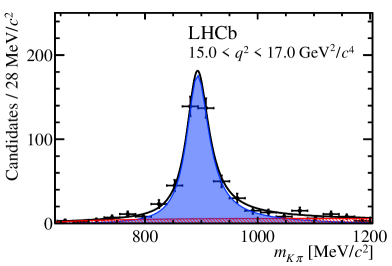
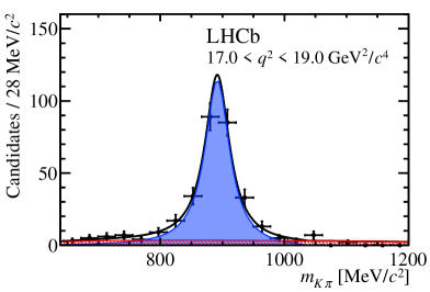
Figure 8: The ${{K}^{+}}{{\pi}^{-}}$ invariant mass distributions for the fine ${q^{2}}$ bins for candidates in the signal $m_{K\pi\mu\mu}$ window of $\pm 50{\mathrm{\,Me\kern-1.00006ptV\!/}c^{2}}$ around the known ${{B}^{0}}$ mass.

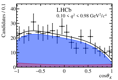
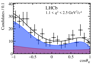
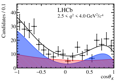
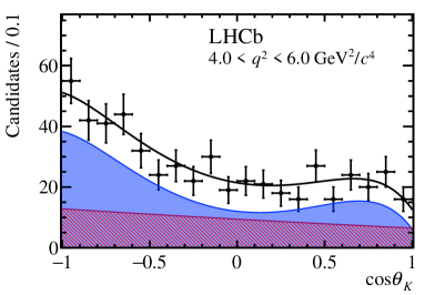
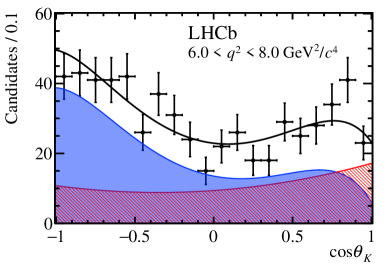
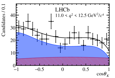
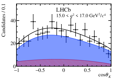
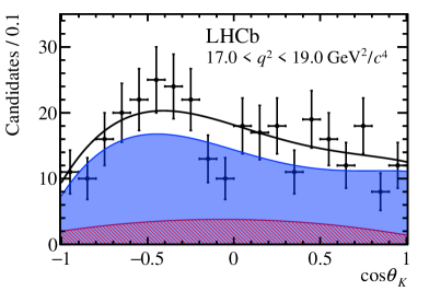
Figure 9: The $\cos{\theta_{K}}$ angular distributions for the fine ${q^{2}}$ bins for candidates in the signal $m_{K\pi\mu\mu}$ window of $\pm 50{\mathrm{\,Me\kern-1.00006ptV\!/}c^{2}}$ around the known ${{B}^{0}}$ mass.

LHCb collaboration

R. Aaij³⁹, B. Adeva³⁸, M. Adinolfi⁴⁷, Z. Ajaltouni⁵, S. Akar⁶, J. Albrecht¹⁰, F. Alessio³⁹, M. Alexander⁵², S. Ali⁴², G. Alkhazov³¹, P. Alvarez Cartelle⁵⁴, A.A. Alves Jr⁵⁸, S. Amato², S. Amerio²³, Y. Amhis⁷, L. An⁴⁰, L. Anderlini¹⁸, G. Andreassi⁴⁰, M. Andreotti^17,g, J.E. Andrews⁵⁹, R.B. Appleby⁵⁵, O. Aquines Gutierrez¹¹, F. Archilli¹, P. d’Argent¹², A. Artamonov³⁶, M. Artuso⁶⁰, E. Aslanides⁶, G. Auriemma^26,s, M. Baalouch⁵, S. Bachmann¹², J.J. Back⁴⁹, A. Badalov³⁷, C. Baesso⁶¹, W. Baldini¹⁷, R.J. Barlow⁵⁵, C. Barschel³⁹, S. Barsuk⁷, W. Barter³⁹, V. Batozskaya²⁹, V. Battista⁴⁰, A. Bay⁴⁰, L. Beaucourt⁴, J. Beddow⁵², F. Bedeschi²⁴, I. Bediaga¹, L.J. Bel⁴², V. Bellee⁴⁰, N. Belloli^21,i, K. Belous³⁶, I. Belyaev³², E. Ben-Haim⁸, G. Bencivenni¹⁹, S. Benson³⁹, J. Benton⁴⁷, A. Berezhnoy³³, R. Bernet⁴¹, A. Bertolin²³, M.-O. Bettler³⁹, M. van Beuzekom⁴², S. Bifani⁴⁶, P. Billoir⁸, T. Bird⁵⁵, A. Birnkraut¹⁰, A. Bitadze⁵⁵, A. Bizzeti^18,u, T. Blake⁴⁹, F. Blanc⁴⁰, J. Blouw¹¹, S. Blusk⁶⁰, V. Bocci²⁶, T. Boettcher⁵⁷, A. Bondar³⁵, N. Bondar^31,39, W. Bonivento¹⁶, S. Borghi⁵⁵, M. Borisyak⁶⁷, M. Borsato³⁸, F. Bossu⁷, M. Boubdir⁹, T.J.V. Bowcock⁵³, E. Bowen⁴¹, C. Bozzi^17,39, S. Braun¹², M. Britsch¹², T. Britton⁶⁰, J. Brodzicka⁵⁵, E. Buchanan⁴⁷, C. Burr⁵⁵, A. Bursche², J. Buytaert³⁹, S. Cadeddu¹⁶, R. Calabrese^17,g, M. Calvi^21,i, M. Calvo Gomez^37,m, P. Campana¹⁹, D. Campora Perez³⁹, L. Capriotti⁵⁵, A. Carbone^15,e, G. Carboni^25,j, R. Cardinale^20,h, A. Cardini¹⁶, P. Carniti^21,i, L. Carson⁵¹, K. Carvalho Akiba², G. Casse⁵³, L. Cassina^21,i, L. Castillo Garcia⁴⁰, M. Cattaneo³⁹, Ch. Cauet¹⁰, G. Cavallero²⁰, R. Cenci^24,t, M. Charles⁸, Ph. Charpentier³⁹, G. Chatzikonstantinidis⁴⁶, M. Chefdeville⁴, S. Chen⁵⁵, S.-F. Cheung⁵⁶, V. Chobanova³⁸, M. Chrzaszcz^41,27, X. Cid Vidal³⁸, G. Ciezarek⁴², P.E.L. Clarke⁵¹, M. Clemencic³⁹, H.V. Cliff⁴⁸, J. Closier³⁹, V. Coco⁵⁸, J. Cogan⁶, E. Cogneras⁵, V. Cogoni^16,f, L. Cojocariu³⁰, G. Collazuol^23,o, P. Collins³⁹, A. Comerma-Montells¹², A. Contu³⁹, A. Cook⁴⁷, S. Coquereau⁸, G. Corti³⁹, M. Corvo^17,g, B. Couturier³⁹, G.A. Cowan⁵¹, D.C. Craik⁵¹, A. Crocombe⁴⁹, M. Cruz Torres⁶¹, S. Cunliffe⁵⁴, R. Currie⁵⁴, C. D’Ambrosio³⁹, E. Dall’Occo⁴², J. Dalseno⁴⁷, P.N.Y. David⁴², A. Davis⁵⁸, O. De Aguiar Francisco², K. De Bruyn⁶, S. De Capua⁵⁵, M. De Cian¹², J.M. De Miranda¹, L. De Paula², P. De Simone¹⁹, C.-T. Dean⁵², D. Decamp⁴, M. Deckenhoff¹⁰, L. Del Buono⁸, M. Demmer¹⁰, D. Derkach⁶⁷, O. Deschamps⁵, F. Dettori³⁹, B. Dey²², A. Di Canto³⁹, H. Dijkstra³⁹, F. Dordei³⁹, M. Dorigo⁴⁰, A. Dosil Suárez³⁸, A. Dovbnya⁴⁴, K. Dreimanis⁵³, L. Dufour⁴², G. Dujany⁵⁵, K. Dungs³⁹, P. Durante³⁹, R. Dzhelyadin³⁶, A. Dziurda³⁹, A. Dzyuba³¹, N. Déléage⁴, S. Easo⁵⁰, U. Egede⁵⁴, V. Egorychev³², S. Eidelman³⁵, S. Eisenhardt⁵¹, U. Eitschberger¹⁰, R. Ekelhof¹⁰, L. Eklund⁵², Ch. Elsasser⁴¹, S. Ely⁶⁰, S. Esen¹², H.M. Evans⁴⁸, T. Evans⁵⁶, A. Falabella¹⁵, N. Farley⁴⁶, S. Farry⁵³, R. Fay⁵³, D. Ferguson⁵¹, V. Fernandez Albor³⁸, F. Ferrari^15,39, F. Ferreira Rodrigues¹, M. Ferro-Luzzi³⁹, S. Filippov³⁴, M. Fiore^17,g, M. Fiorini^17,g, M. Firlej²⁸, C. Fitzpatrick⁴⁰, T. Fiutowski²⁸, F. Fleuret^7,b, K. Fohl³⁹, M. Fontana¹⁶, F. Fontanelli^20,h, D.C. Forshaw⁶⁰, R. Forty³⁹, M. Frank³⁹, C. Frei³⁹, M. Frosini¹⁸, J. Fu^22,q, E. Furfaro^25,j, C. Färber³⁹, A. Gallas Torreira³⁸, D. Galli^15,e, S. Gallorini²³, S. Gambetta⁵¹, M. Gandelman², P. Gandini⁵⁶, Y. Gao³, J. García Pardiñas³⁸, J. Garra Tico⁴⁸, L. Garrido³⁷, P.J. Garsed⁴⁸, D. Gascon³⁷, C. Gaspar³⁹, L. Gavardi¹⁰, G. Gazzoni⁵, D. Gerick¹², E. Gersabeck¹², M. Gersabeck⁵⁵, T. Gershon⁴⁹, Ph. Ghez⁴, S. Gianì⁴⁰, V. Gibson⁴⁸, O.G. Girard⁴⁰, L. Giubega³⁰, K. Gizdov⁵¹, V.V. Gligorov⁸, D. Golubkov³², A. Golutvin^54,39, A. Gomes^1,a, I.V. Gorelov³³, C. Gotti^21,i, M. Grabalosa Gándara⁵, R. Graciani Diaz³⁷, L.A. Granado Cardoso³⁹, E. Graugés³⁷, E. Graverini⁴¹, G. Graziani¹⁸, A. Grecu³⁰, P. Griffith⁴⁶, L. Grillo²¹, O. Grünberg⁶⁵, E. Gushchin³⁴, Yu. Guz³⁶, T. Gys³⁹, C. Göbel⁶¹, T. Hadavizadeh⁵⁶, C. Hadjivasiliou⁶⁰, G. Haefeli⁴⁰, C. Haen³⁹, S.C. Haines⁴⁸, S. Hall⁵⁴, B. Hamilton⁵⁹, X. Han¹², S. Hansmann-Menzemer¹², N. Harnew⁵⁶, S.T. Harnew⁴⁷, J. Harrison⁵⁵, J. He⁶², T. Head⁴⁰, A. Heister⁹, K. Hennessy⁵³, P. Henrard⁵, L. Henry⁸, J.A. Hernando Morata³⁸, E. van Herwijnen³⁹, M. Heß⁶⁵, A. Hicheur², D. Hill⁵⁶, C. Hombach⁵⁵, W. Hulsbergen⁴², T. Humair⁵⁴, M. Hushchyn⁶⁷, N. Hussain⁵⁶, D. Hutchcroft⁵³, M. Idzik²⁸, P. Ilten⁵⁷, R. Jacobsson³⁹, A. Jaeger¹², J. Jalocha⁵⁶, E. Jans⁴², A. Jawahery⁵⁹, M. John⁵⁶, D. Johnson³⁹, C.R. Jones⁴⁸, C. Joram³⁹, B. Jost³⁹, N. Jurik⁶⁰, S. Kandybei⁴⁴, W. Kanso⁶, M. Karacson³⁹, T.M. Karbach^39,†, S. Karodia⁵², M. Kecke¹², M. Kelsey⁶⁰, I.R. Kenyon⁴⁶, M. Kenzie³⁹, T. Ketel⁴³, E. Khairullin⁶⁷, B. Khanji^21,39,i, C. Khurewathanakul⁴⁰, T. Kirn⁹, S. Klaver⁵⁵, K. Klimaszewski²⁹, M. Kolpin¹², I. Komarov⁴⁰, R.F. Koopman⁴³, P. Koppenburg⁴², A. Kozachuk³³, M. Kozeiha⁵, L. Kravchuk³⁴, K. Kreplin¹², M. Kreps⁴⁹, P. Krokovny³⁵, F. Kruse¹⁰, W. Krzemien²⁹, W. Kucewicz^27,l, M. Kucharczyk²⁷, V. Kudryavtsev³⁵, A.K. Kuonen⁴⁰, K. Kurek²⁹, T. Kvaratskheliya^32,39, D. Lacarrere³⁹, G. Lafferty^55,39, A. Lai¹⁶, D. Lambert⁵¹, G. Lanfranchi¹⁹, C. Langenbruch⁴⁹, B. Langhans³⁹, T. Latham⁴⁹, C. Lazzeroni⁴⁶, R. Le Gac⁶, J. van Leerdam⁴², J.-P. Lees⁴, A. Leflat^33,39, J. Lefrançois⁷, R. Lefèvre⁵, F. Lemaitre³⁹, E. Lemos Cid³⁸, O. Leroy⁶, T. Lesiak²⁷, B. Leverington¹², Y. Li⁷, T. Likhomanenko^67,66, R. Lindner³⁹, C. Linn³⁹, F. Lionetto⁴¹, B. Liu¹⁶, X. Liu³, D. Loh⁴⁹, I. Longstaff⁵², J.H. Lopes², D. Lucchesi^23,o, M. Lucio Martinez³⁸, H. Luo⁵¹, A. Lupato²³, E. Luppi^17,g, O. Lupton⁵⁶, A. Lusiani²⁴, X. Lyu⁶², F. Machefert⁷, F. Maciuc³⁰, O. Maev³¹, K. Maguire⁵⁵, S. Malde⁵⁶, A. Malinin⁶⁶, T. Maltsev³⁵, G. Manca⁷, G. Mancinelli⁶, P. Manning⁶⁰, J. Maratas^5,v, J.F. Marchand⁴, U. Marconi¹⁵, C. Marin Benito³⁷, P. Marino^24,t, J. Marks¹², G. Martellotti²⁶, M. Martin⁶, M. Martinelli⁴⁰, D. Martinez Santos³⁸, F. Martinez Vidal⁶⁸, D. Martins Tostes², L.M. Massacrier⁷, A. Massafferri¹, R. Matev³⁹, A. Mathad⁴⁹, Z. Mathe³⁹, C. Matteuzzi²¹, A. Mauri⁴¹, B. Maurin⁴⁰, A. Mazurov⁴⁶, M. McCann⁵⁴, J. McCarthy⁴⁶, A. McNab⁵⁵, R. McNulty¹³, B. Meadows⁵⁸, F. Meier¹⁰, M. Meissner¹², D. Melnychuk²⁹, M. Merk⁴², E Michielin²³, D.A. Milanes⁶⁴, M.-N. Minard⁴, D.S. Mitzel¹², J. Molina Rodriguez⁶¹, I.A. Monroy⁶⁴, S. Monteil⁵, M. Morandin²³, P. Morawski²⁸, A. Mordà⁶, M.J. Morello^24,t, J. Moron²⁸, A.B. Morris⁵¹, R. Mountain⁶⁰, F. Muheim⁵¹, M. Mulder⁴², M. Mussini¹⁵, D. Müller⁵⁵, J. Müller¹⁰, K. Müller⁴¹, V. Müller¹⁰, P. Naik⁴⁷, T. Nakada⁴⁰, R. Nandakumar⁵⁰, A. Nandi⁵⁶, I. Nasteva², M. Needham⁵¹, N. Neri²², S. Neubert¹², N. Neufeld³⁹, M. Neuner¹², A.D. Nguyen⁴⁰, C. Nguyen-Mau^40,n, V. Niess⁵, S. Nieswand⁹, R. Niet¹⁰, N. Nikitin³³, T. Nikodem¹², A. Novoselov³⁶, D.P. O’Hanlon⁴⁹, A. Oblakowska-Mucha²⁸, V. Obraztsov³⁶, S. Ogilvy¹⁹, R. Oldeman⁴⁸, C.J.G. Onderwater⁶⁹, J.M. Otalora Goicochea², A. Otto³⁹, P. Owen⁴¹, A. Oyanguren⁶⁸, A. Palano^14,d, F. Palombo^22,q, M. Palutan¹⁹, J. Panman³⁹, A. Papanestis⁵⁰, M. Pappagallo⁵², L.L. Pappalardo^17,g, C. Pappenheimer⁵⁸, W. Parker⁵⁹, C. Parkes⁵⁵, G. Passaleva¹⁸, G.D. Patel⁵³, M. Patel⁵⁴, C. Patrignani^15,e, A. Pearce^55,50, A. Pellegrino⁴², G. Penso^26,k, M. Pepe Altarelli³⁹, S. Perazzini³⁹, P. Perret⁵, L. Pescatore⁴⁶, K. Petridis⁴⁷, A. Petrolini^20,h, A. Petrov⁶⁶, M. Petruzzo^22,q, E. Picatoste Olloqui³⁷, B. Pietrzyk⁴, M. Pikies²⁷, D. Pinci²⁶, A. Pistone²⁰, A. Piucci¹², S. Playfer⁵¹, M. Plo Casasus³⁸, T. Poikela³⁹, F. Polci⁸, A. Poluektov^49,35, I. Polyakov³², E. Polycarpo², G.J. Pomery⁴⁷, A. Popov³⁶, D. Popov^11,39, B. Popovici³⁰, C. Potterat², E. Price⁴⁷, J.D. Price⁵³, J. Prisciandaro³⁸, A. Pritchard⁵³, C. Prouve⁴⁷, V. Pugatch⁴⁵, A. Puig Navarro⁴⁰, G. Punzi^24,p, W. Qian⁵⁶, R. Quagliani^7,47, B. Rachwal²⁷, J.H. Rademacker⁴⁷, M. Rama²⁴, M. Ramos Pernas³⁸, M.S. Rangel², I. Raniuk⁴⁴, G. Raven⁴³, F. Redi⁵⁴, S. Reichert¹⁰, A.C. dos Reis¹, C. Remon Alepuz⁶⁸, V. Renaudin⁷, S. Ricciardi⁵⁰, S. Richards⁴⁷, M. Rihl³⁹, K. Rinnert^53,39, V. Rives Molina³⁷, P. Robbe^7,39, A.B. Rodrigues¹, E. Rodrigues⁵⁸, J.A. Rodriguez Lopez⁶⁴, P. Rodriguez Perez⁵⁵, A. Rogozhnikov⁶⁷, S. Roiser³⁹, V. Romanovskiy³⁶, A. Romero Vidal³⁸, J.W. Ronayne¹³, M. Rotondo²³, T. Ruf³⁹, P. Ruiz Valls⁶⁸, J.J. Saborido Silva³⁸, N. Sagidova³¹, B. Saitta^16,f, V. Salustino Guimaraes², C. Sanchez Mayordomo⁶⁸, B. Sanmartin Sedes³⁸, R. Santacesaria²⁶, C. Santamarina Rios³⁸, M. Santimaria¹⁹, E. Santovetti^25,j, A. Sarti^19,k, C. Satriano^26,s, A. Satta²⁵, D.M. Saunders⁴⁷, D. Savrina^32,33, S. Schael⁹, M. Schellenberg¹⁰, M. Schiller³⁹, H. Schindler³⁹, M. Schlupp¹⁰, M. Schmelling¹¹, T. Schmelzer¹⁰, B. Schmidt³⁹, O. Schneider⁴⁰, A. Schopper³⁹, K. Schubert¹⁰, M. Schubiger⁴⁰, M.-H. Schune⁷, R. Schwemmer³⁹, B. Sciascia¹⁹, A. Sciubba^26,k, A. Semennikov³², A. Sergi⁴⁶, N. Serra⁴¹, J. Serrano⁶, L. Sestini²³, P. Seyfert²¹, M. Shapkin³⁶, I. Shapoval^17,44,g, Y. Shcheglov³¹, T. Shears⁵³, L. Shekhtman³⁵, V. Shevchenko⁶⁶, A. Shires¹⁰, B.G. Siddi¹⁷, R. Silva Coutinho⁴¹, L. Silva de Oliveira², G. Simi^23,o, M. Sirendi⁴⁸, N. Skidmore⁴⁷, T. Skwarnicki⁶⁰, E. Smith⁵⁴, I.T. Smith⁵¹, J. Smith⁴⁸, M. Smith⁵⁵, H. Snoek⁴², M.D. Sokoloff⁵⁸, F.J.P. Soler⁵², D. Souza⁴⁷, B. Souza De Paula², B. Spaan¹⁰, P. Spradlin⁵², S. Sridharan³⁹, F. Stagni³⁹, M. Stahl¹², S. Stahl³⁹, P. Stefko⁴⁰, S. Stefkova⁵⁴, O. Steinkamp⁴¹, O. Stenyakin³⁶, S. Stevenson⁵⁶, S. Stoica³⁰, S. Stone⁶⁰, B. Storaci⁴¹, S. Stracka^24,t, M. Straticiuc³⁰, U. Straumann⁴¹, L. Sun⁵⁸, W. Sutcliffe⁵⁴, K. Swientek²⁸, V. Syropoulos⁴³, M. Szczekowski²⁹, T. Szumlak²⁸, S. T’Jampens⁴, A. Tayduganov⁶, T. Tekampe¹⁰, G. Tellarini^17,g, F. Teubert³⁹, C. Thomas⁵⁶, E. Thomas³⁹, J. van Tilburg⁴², V. Tisserand⁴, M. Tobin⁴⁰, S. Tolk⁴⁸, L. Tomassetti^17,g, D. Tonelli³⁹, S. Topp-Joergensen⁵⁶, E. Tournefier⁴, S. Tourneur⁴⁰, K. Trabelsi⁴⁰, M. Traill⁵², M.T. Tran⁴⁰, M. Tresch⁴¹, A. Trisovic³⁹, A. Tsaregorodtsev⁶, P. Tsopelas⁴², N. Tuning⁴², A. Ukleja²⁹, A. Ustyuzhanin^67,66, U. Uwer¹², C. Vacca^16,39,f, V. Vagnoni^15,39, S. Valat³⁹, G. Valenti¹⁵, A. Vallier⁷, R. Vazquez Gomez¹⁹, P. Vazquez Regueiro³⁸, S. Vecchi¹⁷, M. van Veghel⁴², J.J. Velthuis⁴⁷, M. Veltri^18,r, G. Veneziano⁴⁰, A. Venkateswaran⁶⁰, M. Vesterinen¹², B. Viaud⁷, D.  Vieira¹, M. Vieites Diaz³⁸, X. Vilasis-Cardona^37,m, V. Volkov³³, A. Vollhardt⁴¹, B Voneki³⁹, D. Voong⁴⁷, A. Vorobyev³¹, V. Vorobyev³⁵, C. Voß⁶⁵, J.A. de Vries⁴², C. Vázquez Sierra³⁸, R. Waldi⁶⁵, C. Wallace⁴⁹, R. Wallace¹³, J. Walsh²⁴, J. Wang⁶⁰, D.R. Ward⁴⁸, N.K. Watson⁴⁶, D. Websdale⁵⁴, A. Weiden⁴¹, M. Whitehead³⁹, J. Wicht⁴⁹, G. Wilkinson^56,39, M. Wilkinson⁶⁰, M. Williams³⁹, M.P. Williams⁴⁶, M. Williams⁵⁷, T. Williams⁴⁶, F.F. Wilson⁵⁰, J. Wimberley⁵⁹, J. Wishahi¹⁰, W. Wislicki²⁹, M. Witek²⁷, G. Wormser⁷, S.A. Wotton⁴⁸, K. Wraight⁵², S. Wright⁴⁸, K. Wyllie³⁹, Y. Xie⁶³, Z. Xing⁶⁰, Z. Xu⁴⁰, Z. Yang³, H. Yin⁶³, J. Yu⁶³, X. Yuan³⁵, O. Yushchenko³⁶, M. Zangoli¹⁵, K.A. Zarebski⁴⁶, M. Zavertyaev^11,c, L. Zhang³, Y. Zhang⁷, Y. Zhang⁶², A. Zhelezov¹², Y. Zheng⁶², A. Zhokhov³², V. Zhukov⁹, S. Zucchelli¹⁵.

¹Centro Brasileiro de Pesquisas Físicas (CBPF), Rio de Janeiro, Brazil
²Universidade Federal do Rio de Janeiro (UFRJ), Rio de Janeiro, Brazil
³Center for High Energy Physics, Tsinghua University, Beijing, China
⁴LAPP, Université Savoie Mont-Blanc, CNRS/IN2P3, Annecy-Le-Vieux, France
⁵Clermont Université, Université Blaise Pascal, CNRS/IN2P3, LPC, Clermont-Ferrand, France
⁶CPPM, Aix-Marseille Université, CNRS/IN2P3, Marseille, France
⁷LAL, Université Paris-Sud, CNRS/IN2P3, Orsay, France
⁸LPNHE, Université Pierre et Marie Curie, Université Paris Diderot, CNRS/IN2P3, Paris, France
⁹I. Physikalisches Institut, RWTH Aachen University, Aachen, Germany
¹⁰Fakultät Physik, Technische Universität Dortmund, Dortmund, Germany
¹¹Max-Planck-Institut für Kernphysik (MPIK), Heidelberg, Germany
¹²Physikalisches Institut, Ruprecht-Karls-Universität Heidelberg, Heidelberg, Germany
¹³School of Physics, University College Dublin, Dublin, Ireland
¹⁴Sezione INFN di Bari, Bari, Italy
¹⁵Sezione INFN di Bologna, Bologna, Italy
¹⁶Sezione INFN di Cagliari, Cagliari, Italy
¹⁷Sezione INFN di Ferrara, Ferrara, Italy
¹⁸Sezione INFN di Firenze, Firenze, Italy
¹⁹Laboratori Nazionali dell’INFN di Frascati, Frascati, Italy
²⁰Sezione INFN di Genova, Genova, Italy
²¹Sezione INFN di Milano Bicocca, Milano, Italy
²²Sezione INFN di Milano, Milano, Italy
²³Sezione INFN di Padova, Padova, Italy
²⁴Sezione INFN di Pisa, Pisa, Italy
²⁵Sezione INFN di Roma Tor Vergata, Roma, Italy
²⁶Sezione INFN di Roma La Sapienza, Roma, Italy
²⁷Henryk Niewodniczanski Institute of Nuclear Physics Polish Academy of Sciences, Kraków, Poland
²⁸AGH - University of Science and Technology, Faculty of Physics and Applied Computer Science, Kraków, Poland
²⁹National Center for Nuclear Research (NCBJ), Warsaw, Poland
³⁰Horia Hulubei National Institute of Physics and Nuclear Engineering, Bucharest-Magurele, Romania
³¹Petersburg Nuclear Physics Institute (PNPI), Gatchina, Russia
³²Institute of Theoretical and Experimental Physics (ITEP), Moscow, Russia
³³Institute of Nuclear Physics, Moscow State University (SINP MSU), Moscow, Russia
³⁴Institute for Nuclear Research of the Russian Academy of Sciences (INR RAN), Moscow, Russia
³⁵Budker Institute of Nuclear Physics (SB RAS) and Novosibirsk State University, Novosibirsk, Russia
³⁶Institute for High Energy Physics (IHEP), Protvino, Russia
³⁷Universitat de Barcelona, Barcelona, Spain
³⁸Universidad de Santiago de Compostela, Santiago de Compostela, Spain
³⁹European Organization for Nuclear Research (CERN), Geneva, Switzerland
⁴⁰Ecole Polytechnique Fédérale de Lausanne (EPFL), Lausanne, Switzerland
⁴¹Physik-Institut, Universität Zürich, Zürich, Switzerland
⁴²Nikhef National Institute for Subatomic Physics, Amsterdam, The Netherlands
⁴³Nikhef National Institute for Subatomic Physics and VU University Amsterdam, Amsterdam, The Netherlands
⁴⁴NSC Kharkiv Institute of Physics and Technology (NSC KIPT), Kharkiv, Ukraine
⁴⁵Institute for Nuclear Research of the National Academy of Sciences (KINR), Kyiv, Ukraine
⁴⁶University of Birmingham, Birmingham, United Kingdom
⁴⁷H.H. Wills Physics Laboratory, University of Bristol, Bristol, United Kingdom
⁴⁸Cavendish Laboratory, University of Cambridge, Cambridge, United Kingdom
⁴⁹Department of Physics, University of Warwick, Coventry, United Kingdom
⁵⁰STFC Rutherford Appleton Laboratory, Didcot, United Kingdom
⁵¹School of Physics and Astronomy, University of Edinburgh, Edinburgh, United Kingdom
⁵²School of Physics and Astronomy, University of Glasgow, Glasgow, United Kingdom
⁵³Oliver Lodge Laboratory, University of Liverpool, Liverpool, United Kingdom
⁵⁴Imperial College London, London, United Kingdom
⁵⁵School of Physics and Astronomy, University of Manchester, Manchester, United Kingdom
⁵⁶Department of Physics, University of Oxford, Oxford, United Kingdom
⁵⁷Massachusetts Institute of Technology, Cambridge, MA, United States
⁵⁸University of Cincinnati, Cincinnati, OH, United States
⁵⁹University of Maryland, College Park, MD, United States
⁶⁰Syracuse University, Syracuse, NY, United States
⁶¹Pontifícia Universidade Católica do Rio de Janeiro (PUC-Rio), Rio de Janeiro, Brazil, associated to ^2
62University of Chinese Academy of Sciences, Beijing, China, associated to ^3
63Institute of Particle Physics, Central China Normal University, Wuhan, Hubei, China, associated to ^3
64Departamento de Fisica , Universidad Nacional de Colombia, Bogota, Colombia, associated to ^8
65Institut für Physik, Universität Rostock, Rostock, Germany, associated to ^12
66National Research Centre Kurchatov Institute, Moscow, Russia, associated to ^32
67Yandex School of Data Analysis, Moscow, Russia, associated to ^32
68Instituto de Fisica Corpuscular (IFIC), Universitat de Valencia-CSIC, Valencia, Spain, associated to ^37
69Van Swinderen Institute, University of Groningen, Groningen, The Netherlands, associated to <sup>42

a</sup>Universidade Federal do Triângulo Mineiro (UFTM), Uberaba-MG, Brazil
^bLaboratoire Leprince-Ringuet, Palaiseau, France
^cP.N. Lebedev Physical Institute, Russian Academy of Science (LPI RAS), Moscow, Russia
^dUniversità di Bari, Bari, Italy
^eUniversità di Bologna, Bologna, Italy
^fUniversità di Cagliari, Cagliari, Italy
^gUniversità di Ferrara, Ferrara, Italy
^hUniversità di Genova, Genova, Italy
ⁱUniversità di Milano Bicocca, Milano, Italy
^jUniversità di Roma Tor Vergata, Roma, Italy
^kUniversità di Roma La Sapienza, Roma, Italy
^lAGH - University of Science and Technology, Faculty of Computer Science, Electronics and Telecommunications, Kraków, Poland
^mLIFAELS, La Salle, Universitat Ramon Llull, Barcelona, Spain
ⁿHanoi University of Science, Hanoi, Viet Nam
^oUniversità di Padova, Padova, Italy
^pUniversità di Pisa, Pisa, Italy
^qUniversità degli Studi di Milano, Milano, Italy
^rUniversità di Urbino, Urbino, Italy
^sUniversità della Basilicata, Potenza, Italy
^tScuola Normale Superiore, Pisa, Italy
^uUniversità di Modena e Reggio Emilia, Modena, Italy
^vIligan Institute of Technology (IIT), Iligan, Philippines
^†Deceased

References

- [1] T. Hurth, F. Mahmoudi, and S. Neshatpour, On the anomalies in the latest LHCb data, arXiv:1603.00865
- [2] S. Descotes-Genon, L. Hofer, J. Matias, and J. Virto, Global analysis of anomalies, arXiv:1510.04239
- [3] S. Descotes-Genon, J. Matias, and J. Virto, Understanding the anomaly, Phys. Rev. D88 (2013) 074002, arXiv:1307.5683
- [4] W. Altmannshofer and D. M. Straub, New physics in ?, Eur. Phys. J. C73 (2013) 2646, arXiv:1308.1501
- [5] F. Beaujean, C. Bobeth, and D. van Dyk, Comprehensive Bayesian analysis of rare (semi)leptonic and radiative decays, Eur. Phys. J. C74 (2014) 2897, arXiv:1310.2478
- [6] T. Hurth and F. Mahmoudi, On the LHCb anomaly in B , JHEP 04 (2014) 097, arXiv:1312.5267
- [7] S. Jäger and J. Martin Camalich, On at small dilepton invariant mass, power corrections, and new physics, JHEP 05 (2013) 043, arXiv:1212.2263
- [8] S. Descotes-Genon, L. Hofer, J. Matias, and J. Virto, On the impact of power corrections in the prediction of observables, JHEP 12 (2014) 125, arXiv:1407.8526
- [9] J. Lyon and R. Zwicky, Resonances gone topsy turvy - the charm of QCD or new physics in ?, arXiv:1406.0566
- [10] W. Altmannshofer, S. Gori, M. Pospelov, and I. Yavin, Quark flavor transitions in models, Phys. Rev. D89 (2014) 095033, arXiv:1403.1269
- [11] A. Crivellin, G. D’Ambrosio, and J. Heeck, Explaining , and in a two-Higgs-doublet model with gauged , Phys. Rev. Lett. 114 (2015) 151801, arXiv:1501.00993
- [12] R. Gauld, F. Goertz, and U. Haisch, An explicit -boson explanation of the anomaly, JHEP 01 (2014) 069, arXiv:1310.1082
- [13] W. Altmannshofer and D. M. Straub, New physics in transitions after LHC run 1, Eur. Phys. J. C75 (2015) 382, arXiv:1411.3161
- [14] F. Mahmoudi, S. Neshatpour, and J. Virto, optimised observables in the MSSM, Eur. Phys. J. C74 (2014) 2927, arXiv:1401.2145
- [15] A. Datta, M. Duraisamy, and D. Ghosh, Explaining the data with scalar interactions, Phys. Rev. D89 (2014) 071501, arXiv:1310.1937
- [16] D. Buttazzo, A. Greljo, G. Isidori, and D. Marzocca, Toward a coherent solution of diphoton and flavor anomalies, arXiv:1604.03940
- [17] M. Ciuchini et al., decays at large recoil in the Standard Model: A theoretical reappraisal, arXiv:1512.07157
- [18] M. Döring, U.-G. Meißner, and W. Wang, Chiral dynamics and S-wave contributions in semileptonic B decays, JHEP 10 (2013) 011, arXiv:1307.0947
- [19] C.-D. Lü and W. Wang, Analysis of in the higher kaon resonance region, Phys. Rev. D85 (2012) 034014, arXiv:1111.1513
- [20] D. Bečirević and A. Tayduganov, Impact of on the New Physics search in decay, Nucl. Phys. B868 (2013) 368, arXiv:1207.4004
- [21] LHCb collaboration, R. Aaij et al., Differential branching fraction and angular analysis of the decay , JHEP 08 (2013) 131, arXiv:1304.6325
- [22] LHCb collaboration, R. Aaij et al., Differential branching fractions and isospin asymmetries of decays, JHEP 06 (2014) 133, arXiv:1403.8044
- [23] CMS collaboration, V. Khachatryan et al., Angular analysis of the decay from collisions at , Phys. Lett. B753 (2016) 424, arXiv:1507.08126
- [24] Belle collaboration, J.-T. Wei et al., Measurement of the differential branching fraction and forward-backword asymmetry for , Phys. Rev. Lett. 103 (2009) 171801, arXiv:0904.0770
- [25] BaBar collaboration, J. P. Lees et al., Measurement of branching fractions and rate asymmetries in the rare decays , Phys. Rev. D86 (2012) 032012, arXiv:1204.3933
- [26] W. Altmannshofer et al., Symmetries and asymmetries of decays in the Standard Model and beyond, JHEP 01 (2009) 019, arXiv:0811.1214
- [27] LHCb collaboration, R. Aaij et al., Angular analysis of the decay using 3 fb-1 of integrated luminosity, JHEP 02 (2016) 104, arXiv:1512.04442
- [28] L. Hofer and J. Matias, Exploiting the symmetries of P and S wave for , JHEP 09 (2015) 104, arXiv:1502.00920
- [29] D. Aston et al., A study of scattering in the reaction at 11, Nucl. Phys. B296 (1988) 493
- [30] LHCb collaboration, A. A. Alves Jr. et al., The LHCb detector at the LHC, JINST 3 (2008) S08005
- [31] R. Aaij et al., Performance of the LHCb Vertex Locator, JINST 9 (2014) P09007, arXiv:1405.7808
- [32] R. Aaij et al., The LHCb trigger and its performance in 2011, JINST 8 (2013) P04022, arXiv:1211.3055
- [33] T. Sjöstrand, S. Mrenna, and P. Skands, PYTHIA 6.4 physics and manual, JHEP 05 (2006) 026, arXiv:hep-ph/0603175
- [34] T. Sjöstrand, S. Mrenna, and P. Skands, A brief introduction to PYTHIA 8.1, Comput. Phys. Commun. 178 (2008) 852, arXiv:0710.3820
- [35] I. Belyaev et al., Handling of the generation of primary events in Gauss, the LHCb simulation framework, J. Phys. Conf. Ser. 331 (2011) 032047
- [36] D. J. Lange, The EvtGen particle decay simulation package, Nucl. Instrum. Meth. A462 (2001) 152
- [37] P. Golonka and Z. Was, PHOTOS Monte Carlo: A precision tool for QED corrections in and decays, Eur. Phys. J. C45 (2006) 97, arXiv:hep-ph/0506026
- [38] M. Clemencic et al., The LHCb simulation application, Gauss: Design, evolution and experience, J. Phys. Conf. Ser. 331 (2011) 032023
- [39] Geant4 collaboration, J. Allison et al., Geant4 developments and applications, IEEE Trans. Nucl. Sci. 53 (2006) 270
- [40] Geant4 collaboration, S. Agostinelli et al., Geant4: A simulation toolkit, Nucl. Instrum. Meth. A506 (2003) 250
- [41] L. Breiman, J. H. Friedman, R. A. Olshen, and C. J. Stone, Classification and regression trees, Wadsworth international group, Belmont, California, USA, 1984
- [42] R. E. Schapire and Y. Freund, A decision-theoretic generalization of on-line learning and an application to boosting, J. Comput. and Syst. Sci. 55 (1997) 119
- [43] LHCb collaboration, R. Aaij et al., Measurement of the branching fraction and angular amplitudes, Phys. Rev. D86 (2012) 071102(R), arXiv:1208.0738
- [44] LHCb collaboration, R. Aaij et al., Observation of the resonant character of the state, Phys. Rev. Lett. 112 (2014) 222002, arXiv:1404.1903
- [45] Particle Data Group, K. A. Olive et al., Review of particle physics, Chin. Phys. C38 (2014) 090001
- [46] D. Das, G. Hiller, M. Jung, and A. Shires, The and distributions at low hadronic recoil, JHEP 09 (2014) 109, arXiv:1406.6681
- [47] D. Das, G. Hiller, and M. Jung, in and outside the window, arXiv:1506.06699
- [48] LHCb collaboration, R. Aaij et al., Measurement of the polarization amplitudes in decays, Phys. Rev. D88 (2013) 052002, arXiv:1307.2782
- [49] Belle collaboration, K. Chilikin et al., Observation of a new charged charmoniumlike state in decays, Phys. Rev. D90 (2014) 112009, arXiv:1408.6457
- [50] A. Bharucha, D. M. Straub, and R. Zwicky, in the Standard Model from light-cone sum rules, arXiv:1503.05534
- [51] R. R. Horgan, Z. Liu, S. Meinel, and M. Wingate, Lattice QCD calculation of form factors describing the rare decays and , Phys. Rev. D89 (2014) 094501, arXiv:1310.3722
- [52] A. Ali, P. Ball, L. T. Handoko, and G. Hiller, A comparative study of the decays in Standard Model and supersymmetric theories, Phys. Rev. D61 (2000) 074024, arXiv:hep-ph/9910221
- [53] P. Ball and R. Zwicky, decay form-factors from light-cone sum rules reexamined, Phys. Rev. D71 (2005) 014029, arXiv:hep-ph/0412079
- [54] A. Khodjamirian, T. Mannel, A. A. Pivovarov, and Y.-M. Wang, Charm-loop effect in and , JHEP 09 (2010) 089, arXiv:1006.4945