Bolt-on Differential Privacy for Scalable
Stochastic Gradient Descent-based Analytics
Abstract
While significant progress has been made separately on analytics systems for scalable stochastic gradient descent (SGD) and private SGD, none of the major scalable analytics frameworks have incorporated differentially private SGD. There are two inter-related issues for this disconnect between research and practice: (1) low model accuracy due to added noise to guarantee privacy, and (2) high development and runtime overhead of the private algorithms. This paper takes a first step to remedy this disconnect and proposes a private SGD algorithm to address both issues in an integrated manner. In contrast to the white-box approach adopted by previous work, we revisit and use the classical technique of output perturbation to devise a novel “bolt-on” approach to private SGD. While our approach trivially addresses (2), it makes (1) even more challenging. We address this challenge by providing a novel analysis of the -sensitivity of SGD, which allows, under the same privacy guarantees, better convergence of SGD when only a constant number of passes can be made over the data. We integrate our algorithm, as well as other state-of-the-art differentially private SGD, into Bismarck, a popular scalable SGD-based analytics system on top of an RDBMS. Extensive experiments show that our algorithm can be easily integrated, incurs virtually no overhead, scales well, and most importantly, yields substantially better (up to 4X) test accuracy than the state-of-the-art algorithms on many real datasets.
1 Introduction
The past decade has seen significant interest from both the data management industry and academia in integrating machine learning (ML) algorithms into scalable data processing systems such as RDBMSs [23, 19], Hadoop [1], and Spark [2]. In many data-driven applications such as personalized medicine, finance, web search, and social networks, there is also a growing concern about the privacy of individuals. To this end, differential privacy, a cryptographically motivated notion, has emerged as the gold standard for protecting data privacy. Differentially private ML has been extensively studied by researchers from the database, ML, and theoretical computer science communities [10, 13, 15, 25, 27, 36, 37].
In this work, we study differential privacy for stochastic gradient descent (SGD), which has become the optimization algorithm of choice in many scalable ML systems, especially in-RDBMS analytics systems. For example, Bismarck [19] offers a highly efficient in-RDBMS implementation of SGD to provide a single framework to implement many convex analysis-based ML techniques. Thus, creating a private version of SGD would automatically provide private versions of all these ML techniques.
While previous work has separately studied in-RDBMS SGD and differentially private SGD, our conversations with developers at several database companies revealed that none of the major in-RDBMS ML tools have incorporated differentially private SGD. There are two inter-related reasons for this disconnect between research and practice: (1) low model accuracy due to the noise added to guarantee privacy, and (2) high development and runtime overhead of the private algorithms. One might expect that more sophisticated private algorithms might be needed to address issue (1) but then again, such algorithms might in turn exacerbate issue (2)!
To understand these issues better, we integrate two state-of-the-art differentially private SGD algorithms – Song, Chaudhuri and Sarwate (SCS13 [35]) and Bassily, Smith and Thakurta (BST14 [10]) – into the in-RDBMS SGD architecture of Bismarck. SCS13 adds noise at each iteration of SGD, enough to make the iterate differentially private. BST14 reduces the amount of noise per iteration by subsampling and can guarantee optimal convergence using passes over the data (where is the training set size); however, in many real applications, we can only afford a constant number of passes, and hence, we derive and implement a version for passes. Empirically, we find that both algorithms suffer from both issues (1) and (2): their accuracy is much worse than the accuracy of non-private SGD, while their “white box” paradigm requires deep code changes that require modifying the gradient update steps of SGD in order to inject noise. In turn, these changes for repeated noise sampling lead to a significant runtime overhead.
In this paper, we take a first step towards mitigating both issues in an integrated manner. In contrast to the white box approach of prior work, we consider a new approach to differentially private SGD in which we treat the SGD implementation as a “black box” and inject noise only at the end. In order to make this bolt-on approach feasible, we revisit and use the classical technique of output perturbation [16]. An immediate consequence is that our approach can be trivially integrated into any scalable SGD system, including in-RDBMS analytics systems such as Bismarck, with no changes to the internal code. Our approach also incurs virtually no runtime overhead and preserves the scalability of the existing system.
While output perturbation obviously addresses the runtime and integration challenge, it is unclear what its effect is on model accuracy. In this work, we provide a novel analysis that leads to an output perturbation procedure with higher model accuracy than the state-of-the-art private SGD algorithms. The essence of our solution is a new bound on the -sensitivity of SGD which allows, under the same privacy guarantees, better convergence of SGD when only a constant number of passes over the data can be made. As a result, our algorithm produces private models that are significantly more accurate than both SCS13 and BST14 for practical problems. Overall, this paper makes the following contributions:
-
•
We propose a novel bolt-on differentially private algorithm for SGD based on output perturbation. An immediate consequence of our approach is that our algorithm directly inherits many desirable properties of SGD, while allowing easy integration into existing scalable SGD-based analytics systems.
-
•
We provide a novel analysis of the -sensitivity of SGD that leads to an output perturbation procedure with higher model accuracy than the state-of-the-art private SGD algorithms. Importantly, our analysis allows better convergence when one can only afford running a constant number of passes over the data, which is the typical situation in practice. Key to our analysis is the use of the well-known expansion properties of gradient operators [29, 31].
-
•
We integrate our private SGD algorithms, SCS13, and BST14 into Bismarck and conduct a comprehensive empirical evaluation. We explain how our algorithms can be easily integrated with little development effort. Using several real datasets, we demonstrate that our algorithms run significantly faster, scale well, and yield substantially better test accuracy (up to 4X) than SCS13 or BST14 for the same settings.
The rest of this paper is organized as follows: In Section 2 we present preliminaries. In Section 3, we present our private SGD algorithms and analyze their privacy and convergence guarantees. Along the way, we extend our main algorithms in various ways to incorporate common practices of SGD. We then perform a comprehensive empirical study in Section 4 to demonstrate that our algorithms satisfy key desired properties for in-RDBMS analytics: ease of integration, low runtime overhead, good scalability, and high accuracy. We provide more remarks on related theoretical work in Section 5 and conclude with future directions in Section 6.
2 Preliminaries
This section reviews important definitions and existing results.
Machine Learning and Convex ERM. Focusing on supervised learning, we have a sample space , where is a space of feature vectors and is a label space. We also have an ordered training set . Let be a hypothesis space equipped with the standard inner product and 2-norm . We are given a loss function which measures the how well a classifies an example , so that given a hypothesis and a sample , we have a loss . Our goal is to minimize the empirical risk over the training set (i.e., the empirical risk minimization, or ERM), defined as . Fixing , is a function of . In both in-RDBMS and private learning, convex ERM problems are common, where every is convex. We start by defining some basic properties of loss functions that will be needed later to present our analysis.
Definition 1.
Let be a function:
-
•
is convex if for any ,
-
•
is -Lipschitz if for any ,
-
•
is -strongly convex if
-
•
is -smooth if
Example: Logistic Regression. The above three parameters (, , and ) are derived by analyzing the loss function. We give an example using the popular -regularized logistic regression model with the regularization parameter . This derivation is standard in the optimization literature (e.g., see [11]). We assume some preprocessing that normalizes each feature vector, i.e., each (this assumption is common for analyzing private optimization [10, 13, 35]. In fact, such preprocessing are also common for general machine learning problems [6], not just private ones). Recall now that for -regularized logistic regression the loss function on an example with ) is defined as follows:
| (1) |
Fixing , we can obtain , , and by looking at the expression for the gradient () and the Hessian (). is chosen as a tight upper bound on , is chosen as a tight upper bound on , and is chosen such that , i.e., is positive semidefinite).
Now there are two cases depending on whether or not. If we do not have strong convexity (in this case it is only convex), and we have and . If , we need to assume a bound on the norm of the hypothesis . (which can be achieved by rescaling). In particular, suppose , then together with , we can deduce that , , and . We remark that these are indeed standard values in the literature for -regularized logistic loss [11].
The above assumptions and derivation are common in the optimization literature [11, 12]. In some ML models, is not differentiable, e.g., the hinge loss for the linear SVM [4]. The standard approach in this case is to approximate it with a differentiable and smooth function. For example, for the hinge loss, there is a body of work on the so-called Huber SVM [4]. In this paper, we focus primarily on logistic regression as our example but we also discuss the Huber SVM and present experiments for it in the appendix.
Stochastic Gradient Descent. SGD is a simple but popular optimization algorithm that performs many incremental gradient updates instead of computing the full gradient of . At step , given and a random example , SGD’s update rule is as follows:
| (2) |
where is the loss function and is a parameter called the learning rate, or step size. We will denote as . A form of SGD that is commonly used in practice is permutation-based SGD (PSGD): first sample a random permutation of ( is the size of the training set ), and then repeatedly apply (2) by cycling through according to . In particular, if we cycle through the dataset times, it is called -pass PSGD.
We now define two important properties of gradient updates that are needed to understand the analysis of SGD’s convergence in general, as well as our new technical results on differentially private SGD: expansiveness and boundedness. Specifically, we use these definitions to introduce a simple but important recent optimization-theoretical result on SGD’s behavior by [21] that we adapt and apply to our problem setting. Intuitively, expansiveness tells us how much can expand or contract the distance between two hypotheses, while boundedness tells us how much modifies a given hypothesis. We now provide the formal definitions (due to [29, 31]).
Definition 2 (Expansiveness).
Let be an operator that maps a hypothesis to another hypothesis. is said to be -expansive if
Definition 3 (Boundedness).
Let be an operator that maps a hypothesis to another hypothesis. is said to be -bounded if
Lemma 1 (Expansiveness ([29, 31])).
Assume that is -smooth. Then, the following hold.
-
1.1.
If is convex, then for any , is -expansive.
-
1.2.
If is -strongly convex, then for , is -expansive.
In particular we use the following simplification due to [21].
Lemma 2 ([21]).
Suppose that is -smooth and -strongly convex. If , then is -expansive.
Lemma 3 (Boundedness).
Assume that is -Lipschitz. Then the gradient update is -bounded.
We are ready to describe a key quantity studied in this paper.
Definition 4 ().
Let , and be two sequences in . We define as .
The following lemma by Hardt, Recht and Singer [21] bounds using expansiveness and boundedness properties (Lemma 1 and 3).
Lemma 4 (Growth Recursion [21]).
Fix any two sequences of updates and . Let and and for . Then
Essentially, Lemma 4 is used as a tool to prove “average-case stability” of standard SGD in [21]. We adapt and apply this result to our problem setting and devise new differentially private SGD algorithms.111 Interestingly, differential privacy can be viewed as notion of “worst-case stability.” Thus we offer “worst-case stability.” The application is non-trivial because of our unique desiderata but we achieve it by leveraging other recent important optimization-theoretical results by [34] on the convergence of PSGD. Overall, by synthesizing and building on these recent results, we are able to prove the convergence of our private SGD algorithms as well.
Differential Privacy. We say that two datasets are neighboring, denoted by , if they differ on a single individual’s private value. Recall the following definition:
Definition 5 (-differential privacy).
A (randomized) algorithm is said to be -differentially private if for any neighboring datasets , and any event ,
In particular, if , we will use -differential privacy instead of -differential privacy. A basic paradigm to achieve -differential privacy is to examine a query’s -sensitivity,
Definition 6 (-sensitivity).
Let be a deterministic query that maps a dataset to a vector in . The -sensitivity of is defined to be
The following theorem relates -differential privacy and -sensitivity.
Theorem 1 ([16]).
Let be a deterministic query that maps a database to a vector in . Then publishing where is sampled from the distribution with density
| (3) |
ensures -differential privacy.
For the interested reader, we provide a detailed algorithm in Appendix E for how to sample from the above distribution.
Importantly, the -norm of the noise vector, , is distributed according to the Gamma distribution . We have the following fact about Gamma distributions:
Theorem 2 ([13]).
For the noise vector , we have that with probability at least ,
Note that the noise depends linearithmically on . This could destroy utility (lower accuracy dramatically) if is high. But there are standard techniques to mitigate this issue that are commonly used in private SGD literature (we discuss more in Section 4.3). By switching to Gaussian noise, we obtain -differential privacy.
Theorem 3 ([17]).
Let be a deterministic query that maps a database to a vector in . Let be arbitrary. For , adding Gaussian noise sampled according to
| (4) |
ensures -differentially privacy.
For Gaussian noise, the dependency on is , instead of .
Random Projection. Known convergence results of private SGD (in fact private ERM in general) have a poor dependencies on the dimension . To handle high dimensions, a useful technique is random projection [7]. That is, we sample a random linear transformation from certain distributions and apply to each feature point in the training set, so is transformed to . Note that after this transformation two neighboring datasets (datasets differing at one data point) remain neighboring, so random projection does not affect our privacy analysis. Further, the theory of random projection will tell “what low dimension” to project to so that “approximate utility will be preserved.” (in our MNIST experiments the accuracy gap between original and projected dimension is very small). Thus, for problems with higher dimensions, we invoke the random projection to “lower” the dimension to achieve small noise and thus better utility, while preserving privacy.
In our experimental study we apply random projection to one of our datasets (MNIST).
3 Private SGD
We present our differentially private PSGD algorithms and analyze their privacy and convergence guarantees. Specifically, we present a new analysis of the output perturbation method for PSGD. Our new analysis shows that very little noise is needed to achieve differential privacy. In fact, the resulting private algorithms have good convergence rates with even one pass over the data. Since output perturbation also uses standard PSGD algorithm as a black-box, this makes our algorithms attractive for in-RDBMS scenarios.
This section is structured accordingly in two parts. In Section 3.1 we give two main differentially private algorithms for convex and strongly convex optimization. In Section 3.2 we first prove that these two algorithms are differentially private (Section 3.2.1 and 3.2.2), then extend them in various ways (Section 3.2.3), and finally prove their convergence (Section 3.2.4).
3.1 Algorithms
As we mentioned before, our differentially private PSGD algorithms uses one of the most basic paradigms for achieving differential privacy – the output perturbation method [16] based on -sensitivity (Definition 6). Specifically, our algorithms are “instantiations” of the output perturbation method where the -sensitivity parameter 2 is derived using our new analysis. To describe the algorithms, we assume a standard permutation-based SGD procedure (denoted as PSGD) which can be invoked as a black-box. To facilitate the presentation, Table 1 summarizes the parameters.
| Symbol | Meaning |
|---|---|
| -regularization parameter. | |
| Lipschitz constant. | |
| Strong convexity. | |
| Smoothness. | |
| Privacy parameters. | |
| Learning rate or step size at iteration . | |
| A convex set that forms the hypothesis space. | |
| Radius of the hypothesis space . | |
| Number of passes through the data. | |
| Mini-batch size of SGD. | |
| Size of the training set . |
Algorithms 1 and 2 give our private SGD algorithms for convex and strongly convex cases, respectively. A key difference between these two algorithms is at line 5 where different -sensitivities are used to sample the noise . Note that different learning rates are used: In the convex case, a constant rate is used, while a decreasing rate is used in the strongly convex case. Finally, note that the standard PSGD is invoked as a black box at line 4.
3.2 Analysis
In this section we investigate privacy and convergence guarantees of Algorithms 1 and 2. Along the way, we also describe extensions to accommodate common practices in running SGD. Most proofs in this section are deferred to the appendix.
Overview of the Analysis and Key Observations. For privacy, let denote a randomized non-private algorithm where denotes the randomness (e.g., random permutations sampled by SGD) and denotes the input training set. To bound -sensitivity we want to bound on a pair of neighboring datasets , where can be different randomness sequences of in general. This can be complicated since and may access the data in vastly different patterns.
Our key observation is that for non-adaptive randomized algorithms, it suffices to consider randomness sequences one at a time, and thus bound . This in turn allows us to obtain a small upper bound of the -sensitivity of SGD by combining the expansion properties of gradient operators and the fact that one will only access once the differing data point between and for each pass over the data, if is a random permutation.
Finally for convergence, while using permutation benefits our privacy proof, the convergence behavior of permutation-based SGD is poorly understood in theory. Fortunately, based on very recent advances by Shamir [34] on the sampling-without-replacement SGD, we prove convergence of our private SGD algorithms even with only one pass over the data.
Randomness One at a Time. Consider the following definition,
Definition 7 (Non-Adaptive Algorithms).
A randomized algorithm is non-adaptive if its random choices do not depend on the input data values.
PSGD is clearly non-adaptive as a single random permutation is sampled at the very beginning of the algorithm. Another common SGD variant, where one independently and uniformly samples at iteration and picks the -th data point, is also non-adaptive. In fact, more modern SGD variants, such as Stochastic Variance Reduced Gradient (SVRG [26]) and Stochastic Average Gradient (SAG [32]), are non-adaptive as well. Now we have the following lemma for non-adaptive algorithms and differential privacy.
Lemma 5.
Let be a non-adaptive randomized algorithm where denotes the randomness of the algorithm and denotes the dataset works on. Suppose that
Then publishing where is sampled with density ensures -differential privacy.
Proof.
Let denote the private version of . has two parts of randomness: One part is , which is used to compute ; the second part is , which is used for perturbation (i.e. ). Let be the random variable corresponding to the randomness of . Note that does not depend on the input training set. Thus for any event ,
| (5) | ||||
Denote by . Then similarly for we have that
| (6) | ||||
Compare (LABEL:eq:1) and (LABEL:eq:2) term by term (for every ): the lemma then follows as we calibrate the noise so that . ∎
From now on we denote PSGD by . With the notations in Definition 4, our next goal is thus to bound . In the next two sections we bound this quantity for convex and strongly convex optimization, respectively.
3.2.1 Convex Optimization
In this section we prove privacy guarantee when is convex. Recall that for general convex optimization, we have -expansiveness by Lemma 1.1. We thus have the following lemma that bounds .
Lemma 6.
Consider -passes PSGD for -Lipschitz, convex and -smooth optimization where for . Let be any neighboring datasets. Let be a random permutation of . Suppose that . Let , then
We immediately have the following corollary on -sensitivity with constant step size,
Corollary 1 (Constant Step Size).
Consider -passes PSGD for -Lipschitz, convex and -smooth optimization. Suppose further that we have constant learning rate . Then
This directly yields the following theorem,
Theorem 4.
Algorithm 1 is -differentially private.
We now give -sensitivity results for two different choices of step sizes, which are also common for convex optimization.
Corollary 2 (Decreasing Step Size).
Let be some constant. Consider -passes PSGD for -Lipschitz, convex and -smooth optimization. Suppose further that we take decreasing step size where is the training set size. Then .
Corollary 3 (Square-Root Step Size).
Let be some constant. Consider -passes PSGD for -Lipschitz, convex and -smooth optimization. Suppose further that we take square-root step size . Then
Remark on Constant Step Size. In Lemma 1 the step size is named “constant” for the SGD. However, one should note that Constant step size for SGD can depend on the size of the training set, and in particular can vanish to zero as training set size increases. For example, a typical setting of step size is (In fact, in typical convergence results of SGD, see, for example in [12, 28], the constant step size is set to where is the total number of iterations). This, in particular, implies a sensitivity , which vanishes to as grows to infinity.
3.2.2 Strongly Convex Optimization
Now we consider the case where is -strongly convex. In this case the sensitivity is smaller because the gradient operators are -expansive for so in particular they become contractions. We have the following lemmas.
Lemma 7 (Constant Step Size).
Consider PSGD for -Lipschitz, -strongly convex and -smooth optimization with constant step sizes . Let be the number of passes. Let be two neighboring datasets differing at the -th data point. Let be a random permutation of . Suppose that . Let , then In particular,
Lemma 8 (Decreasing Step Size).
Consider -passes PSGD for -Lipschitz, -strongly convex and -smooth optimization. Suppose further that we use decreasing step length: . Let be two neighboring datasets differing at the -th data point. Let be a random permutation of . Suppose that . Let , then
In particular, Lemma 8 yields the following theorem,
Theorem 5.
Algorithm 2 is -differentially private.
One should contrast this theorem with Theorem 4: In the convex case we bound -sensitivity by , while in the strongly convex case we bound it by
3.2.3 Extensions
In this section we extend our main argument in several ways: -differential privacy, mini-batching, model averaging, fresh permutation at each pass, and finally constrained optimization. These extensions can be easily incorporated to standard PSGD algorithm, as well as our private algorithms 1 and 2, and are used in our empirical study later.
-Differential Privacy. We can also obtain -differential privacy easily using Gaussian noise (see Theorem 3).
Lemma 9.
Let be a non-adaptive randomized algorithm where denotes the randomness of the algorithm and denote the dataset. Suppose that
Then for any , publishing where each component of is sampled using (4) ensures -differential privacy.
In particular, combining this with our -sensitivity results, we get the following two theorems,
Theorem 6 (Convex and Constant Step).
Theorem 7 (Strongly Convex and Decreasing Step).
Mini-batching. A popular way to do SGD is that at each step, instead of sampling a single data point and do gradient update w.r.t. it, we randomly sample a batch of size , and do
For permutation SGD, a natural way to employ mini-batch is to partition the data points into mini-batches of size (for simplicity let us assume that divides ), and do gradient updates with respect to each chunk. In this case, we notice that mini-batch indeed improves the sensitivity by a factor of . In fact, let us consider neighboring datasets , and at step , we have batches that differ in at most one data point. Without loss of generality, let us consider the case where differ at one data point, then on we have and on we have and so
We note that for all except one in , , and so by the Growth Recursion Lemma 4, if is -expansive, and for the differing index , . Therefore, for a uniform bound on expansiveness and on boundedness (for all , which is the case in our analysis), we have that This implies a factor improvement for all our sensitivity bounds.
Model Averaging. Model averaging is a popular technique for SGD. For example, given iterates , a common way to do model averaging is either to output or output the average of the last iterates. We show that model averaging will not affect our sensitivity result, and in fact it will give a constant-factor improvement when earlier iterates have smaller sensitivities. We have the following lemma.
Lemma 10 (Model Averaging).
Suppose that instead of returning at the end of the optimization, we return an averaged model where is a sequence of coefficients that only depend on . Then,
In particular, we notice that the ’s we derived before are non-decreasing, so the sensitivity is bounded by .
Fresh Permutation at Each Pass. We note that our analysis extends verbatim to the case where in each pass a new permutation is sampled, as our analysis applies to any fixed permutation.
Constrained Optimization. Until now, our SGD algorithm is for unconstrained optimization. That is, the hypothesis space is the entire . Our results easily extend to constrained optimization where the hypothesis space is a convex set . That is, our goal is to compute . In this case, we change the original gradient update rule 2 to the projected gradient update rule:
| (7) |
where is the projection of to . It is easy to see that our analysis carries over verbatim to the projected gradient descent. In fact, our analysis works as long as the optimization is carried over a Hilbert space (i.e., the is induced by some inner product). The essential reason is that projection will not increase the distance (), and thus will not affect our sensitivity argument.
3.2.4 Convergence of Optimization
We now bound the optimization error of our private PSGD algorithms. More specifically, we bound the excess empirical risk where is the loss of the output of our private SGD algorithm and is the minimum obtained by any in the feasible set . Note that in PSGD we sample data points without replacement. While sampling without replacement benefits our -sensitivity argument, its convergence behavior is poorly understood in theory. Our results are based on very recent advances by Shamir [34] on the sampling-without-replacement SGD.
As in Shamir [34], we assume that the loss function takes the form of where is some fixed function. Further we assume that the optimization is carried over a convex set of radius (i.e., for ). We use projected PSGD algorithm (i.e., we use the projected gradient update rule 7).
Finally, is a regret bound if for any and convex-Lipschitz , and is sublinear in . We use the following regret bound,
Theorem 8 (Zinkevich [38]).
For SGD with constant step size , is bounded by .
The following lemma is useful in bounding excess empirical risk.
Lemma 11 (Risk due to Privacy).
Consider -Lipschitz and -smooth optimization. Let be the output of the non-private SGD algorithm, be the noise of the output perturbation, and . Then
-Differential Privacy. We now give convergence result for SGD with -differential privacy.
Convex Optimization. If is convex, we use the following theorem from Shamir [34],
Theorem 9 (Corollary 1 of Shamir [34]).
Let (that is we take at most -pass over the data). Suppose that each iterate is chosen from , and the SGD algorithm has regret bound , and that , and for all . Finally, suppose that each loss function takes the form for some -Lipschitz and , and a fixed , then
Together with Theorem 8, we thus have the following lemma,
Lemma 12.
Now we can bound the excess empirical risk as follows,
Theorem 10 (Convex and Constant Step Size).
Note that the term corresponds to the expectation of .
Strongly Convex Optimization. If is -strongly convex, we instead use the following theorem,
Theorem 11 (Theorem 3 of Shamir [34]).
Suppose has diameter , and is -strongly convex on . Assume that each loss function takes the for where , is possibly some regularization term, and each is -Lipschitz and -smooth. Furthermore, suppose . Then for any , if we run SGD for iterations with step size , we have
where is some universal positive constant.
By the same argument as in the convex case, we have,
Theorem 12 (Strongly Convex and Decreasing Step Size).
Consider the same setting as in Theorem 11 where the step size is . Consider -pass PSGD. Let be the result of model averaging and be the result of output perturbation. Then
Remark. Our convergence results for -differential privacy is different from previous work, such as BST14, which only give convergence for -differential privacy for . In fact, BST14 relies in an essential way on the advanced composition of -differential privacy [17] and we are not aware its convergence for -differential privacy. Note that -differential privacy is qualitatively different from -differential privacy (see, for example, paragraph 3, pp. 18 in Dwork and Roth [17], as well as a recent article by McSherry [5]). We believe that our convergence results for -differential privacy is important in its own right.
-Differential Privacy. By replacing Laplace noise with Gaussian noise, we can derive similar convergence results of our algorithms for -differential privacy for -pass SGD.
It is now instructive to compare our convergence results with BST14 for constant number of passes. In particular, by plugging in different parameters into the analysis of BST14 (in particular, Lemma 2.5 and Lemma 2.6 in BST14) one can derive variants of their results for constant number of passes. The following table compares the convergence in terms of the dependencies on the number of training points , and the number of dimensions .
| Ours | BST14 | |
|---|---|---|
| Convex | ||
| Strongly Convex |
In particular, in the convex case our convergence is better with a factor, and in the strongly convex case ours is better with a factor. These logarithmic factors are inherent in BST14 due to its dependence on some optimization results (Lemma 2.5, 2.6 in their paper), which we do not rely on. Therefore, this comparison gives theoretical evidence that our algorithms converge better for constant number passes. On the other hand, these logarithmic factors become irrelevant for BST14 with passes, as the denominator becomes in the convex case, and becomes in the strongly case, giving better dependence on there.
4 Implementation and Evaluation
In this section, we present a comprehensive empirical study comparing three alternatives for private SGD: two previously proposed state-of-the-art private SGD algorithms, SCS13 [35] and BST14 [10], and our algorithms which are instantiations of the output perturbation method with our new analysis.
Our goal is to answer four main questions associated with the key desiderata of in-RDBMS implementations of private SGD, viz., ease of integration, runtime overhead, scalability, and accuracy:
-
1.
What is the effort to integrate each algorithm into an in-RDBMS analytics system?
-
2.
What is the runtime overhead and scalability of the private SGD implementations?
-
3.
How does the test accuracy of our algorithms compare to SCS13 and BST14?
-
4.
How do various parameters affect the test accuracy?
As a summary, our main findings are the following: (i) Our SGD algorithms require almost no changes to Bismarck, while both SCS13 and BST14 require deeper code changes. (ii) Our algorithms incur virtually no runtime overhead, while SCS13 and BST14 run much slower. Our algorithms scale linearly with the dataset size. While SCS13 and BST14 also enjoy linear scalability, the runtime overhead they incur also increases linearly. (iii) Under the same differential privacy guarantees, our private SGD algorithms yield substantially better accuracy than SCS13 and BST14, for all datasets and settings of parameters we test. (iv) As for the effects of parameters, our empirical results align well with the theory. For example, as one might expect, mini-batch sizes are important for reducing privacy noise. The number of passes is more subtle. For our algorithm, if the learning task is only convex, more passes result in larger noise (e.g., see Lemma 1), and so give rise to potentially worse test accuracy. On the other hand, if the learning task is strongly convex, the number of passes will not affect the noise magnitude (e.g., see Lemma 8). As a result, doing more passes may lead to better convergence and thus potentially better test accuracy. Interestingly, we note that slightly enlarging mini-batch size can reduce noise very effectively so it is affordable to run our private algorithms for more passes to get better convergence in the convex case. This corroborates the results of [35] that mini-batches are helpful in private SGD settings.
In the rest of this section we give more details of our evaluation. Our discussion is structured as follows: In Section 4.1 we first discuss the implemented algorithms. In particular, we discuss how we modify SCS13 and BST14 to make them better fit into our experiments. We also give some remarks on other relevant previous algorithms, and on parameter tuning. Then in Section 4.2 we discuss the effort of integrating different algorithms into Bismarck. Next Section 4.3 discusses the experimental design and datasets for runtime overhead, scalability and test accuracy. Then in Section 4.4, we report runtime overhead and scalability results. We report test accuracy results for various datasets and parameter settings, and discuss the effects of parameters in Section 4.5. Finally, we discuss the lessons we learned from our experiments 4.6.
4.1 Implemented Algorithms
We first discuss implementations of our algorithms, SCS13 and BST14. Importantly, we extend both SCS13 and BST14 to make them better fit into our experiments. Among these extensions, probably most importantly, we extend BST14 to support a smaller number of iterations through the data and reduce the amount of noise needed for each iteration. Our extension makes BST14 more competitive in our experiments.
Our Algorithms. We implement Algorithms 1 and 2 with the extensions of mini-batching and constrained optimization (see Section 3.2.3). Note that Bismarck already supports standard PSGD algorithm with mini-batching and constrained optimization. Therefore the only change we need to make for Algorithms 1 and 2 (note that the total number of updates is ) is the setting of -sensitivity parameter 2 at line 5 of respective algorithms, which we divide by if the mini-batch size is .
SCS13 [35]. We modify [35], which originally only supports one pass through the data, to support multi-passes over the data.
BST14 [10]. BST14 provides a second solution for private SGD following the same paradigm as SCS13, but with less noise per iteration. This is achieved by first, using a novel subsampling technique and second, relaxing the privacy guarantee to -differential privacy for . This relaxation is necessary as they need to use advanced composition results for -differential privacy.
However, the original BST14 algorithm needs iterations to finish, which is prohibitive for even moderate sized datasets. We extend it to support iterations for some constant . Reducing the number of iterations means that potentially we can reduce the amount of noise for privacy because data is “less examined.” This is indeed the case: One can go through the same proof in [10] with a smaller number of iterations, and show that each iteration only needs a smaller amount of noise than before (unfortunately this does not give convergence results). Our extension makes BST14 more competitive. In fact it yields significantly better test accuracy compared to the case where one naïvely stops BST14 after passes, but the noise magnitude in each iteration is the same as in the original paper [10] (which is for passes). The extended BST14 algorithms are given in Algorithm 4 and 5. Finally, we also make straightforward extensions so that BST14 supports mini-batching.
Other Related Work. We also note the work of Jain, Kothari and Thakurta [24] which is related to our setting. In particular their Algorithm 6 is similar to our private SGD algorithm in the setting of strong convexity and -differential privacy. However, we note that their algorithm uses Implicit Gradient Descent (IGD), which belongs to proximal algorithms (see for example Parikh and Boyd [30]) and is known to be more difficult to implement than stochastic gradient methods. Due to this consideration, in this study we will not compare empirically with this algorithm. Finally, we also note that [24] also has an SGD-style algorithm (Algorithm 3) for strongly convex optimization and -differential privacy. This algorithm adds noise comparable to our algorithm at each step of the optimization, and thus we do not compare with it either.
Private Parameter Tuning. We observe that for all SGD algorithms considered, it may be desirable to fine tune some parameters to achieve the best performance. For example, if one chooses to do -regularization, then it is customary to tune the parameter . We note that under the theme of differential privacy, such parameter tunings must also be done privately. To the best of our knowledge however, no previous work have evaluated the effect of private parameter tuning for SGD. Therefore we take the natural step to fill in this gap. We note that there are two possible ways to do this.
Tuning using Public Data. Suppose that one has access to a public data set, which is assumed to be drawn from the same distribution as the private data set. In this case, one can use standard methods to tune SGD parameters, and apply the parameters to the private data.
Tuning using a Private Tuning Algorithm. When only private data is available, we use a private tuning algorithm for private parameter tuning. Following the principle on free parameters [22] in experimenting with differential privacy, we note free parameters . For these parameters, are specified as privacy guarantees. Following common practice for constrained optimization (e.g. [35]) we set for numeric stability. Thus the parameters we need to tune are . We call the tuning parameters. We use a standard grid search [3] with commonly used values to define the space of parameter values, from which the tuning algorithm picks values for the parameters to tune.
We use the tuning algorithm described in the original paper of Chaudhuri, Monteleoni and Sarwate [13], though the methodology and experiments in the following are readily extended to other private tuning algorithms [14]. Specifically, let denote a tuple of the tuning parameters. Given a space , Algorithm 3 gives the details of the tuning algorithm.
4.2 Integration with Bismarck
We now explain how we integrate private SGD algorithms in RDBMS. To begin with, we note that the state-of-the-art way to do in-RDBMS data analysis is via the User Defined Aggregates (UDA) offered by almost all RDBMSes [20]. Using UDAs enables scaling to larger-than-memory datasets seamlessly while still being fast.222The MapReduce abstraction is similar to an RDBMS UDA [1]. Thus our implementation ideas apply to MapReduce-based systems as well. A well-known open source implementation of the UDAs required is Bismarck [19]. Bismarck achieves high performance and scalability through a unified architecture of in-RDBMS data analytics systems using the permutation-based SGD.
Therefore, we use Bismarck to experiment with private SGD inside RDBMS. Specifically, we use Bismarck on top of PostgreSQL, which implements the UDA for SGD in C to provide high runtime efficiency. Our results carry over naturally to any other UDA-based implementation of analytics in an RDBMS. The rest of this section is organized as follows. We first describe Bismarck’s system architecture. We then compare the system extensions and the implementation effort needed for integrating our private PSGD algorithm as well as SCS13 and BST14.
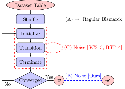
Figure 1 (A) gives an overview of Bismarck’s architecture. The dataset is stored as a table in PostgreSQL. Bismarck permutes the table using an SQL query with a shuffling clause, viz., ORDER BY RANDOM(). A pass (or epoch, which is used more often in practice) of SGD is implemented as a C UDA and this UDA is invoked with an SQL query for each epoch. A front-end controller in Python issues the SQL queries and also applies the convergence test for SGD after each epoch. The developer has to provide implementations of three functions in the UDA’s C API: , , and , all of which operate on the , which is the quantity being computed.
To explain how this works, we compare SGD with a standard SQL aggregate: AVG. The state for AVG is the 2-tuple , while that for SGD is the model vector . The function sets for AVG, while for SGD, it sets to the value given by the Python controller (the previous epoch’s output model). The function updates the state based on a single tuple (one example). For example, given a tuple with value , the state update for AVG is as follows: . For SGD, is the feature vector and the update is the update rule for SGD with the gradient on . If mini-batch SGD is used, the updates are made to a temporary accumulated gradient that is part of the aggregation state along with counters to track the number of examples and mini-batches seen so far. When a mini-batch is over, the function updates using the accumulated gradient for that mini-batch using an appropriate step size. The function computes and outputs it for AVG, while for SGD, it simply returns at the end of that epoch.
It is easy to see that our private SGD algorithm requires almost no change to Bismarck – simply add noise to the final output after all epochs, as illustrated in Figure 1 (B). Thus, our algorithm does not modify any of the RDBMS-related C UDA code. In fact, we were able to implement our algorithm in about 10 lines of code (LOC) in Python within the front-end Python controller. In contrast, both SCS13 and BST14 require deeper changes to the UDA’s function because they need to add noise at the end of each mini-batch update. Thus, implementing them required adding dozens of LOC in C to implement their noise addition procedure within the function, as illustrated in Figure 1 (C). Furthermore, Python’s scipy library already provides the sophisticated distributions needed for sampling the noise (gamma and multivariate normal), which our algorithm’s implementation exploits. But for both SCS13 and BST14, we need to implement some of these distributions in C so that it can be used in the UDA.333One could use the Python-based UDAs in PostgreSQL but that incurs a significant runtime performance penalty compared to C UDAs.
4.3 Experimental Method and Datasets
We now describe our experimental method and datasets.
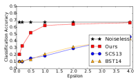
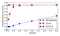
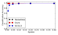
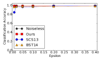
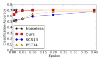
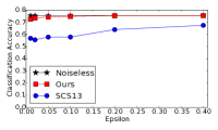
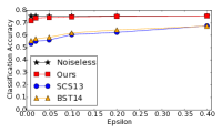
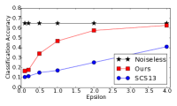
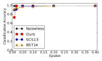
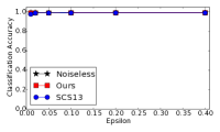
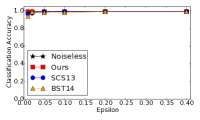
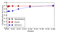
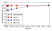
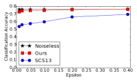
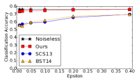
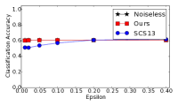
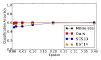
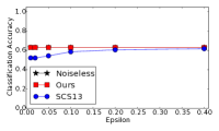
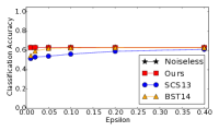
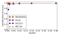
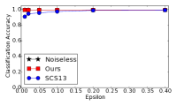
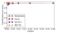
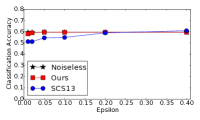
Test Scenarios. We consider four main scenarios to evaluate the algorithms: (1) Convex, -differential privacy, (2) Convex, -differential privacy, (3) Strongly Convex, -differential privacy, and finally (4) Strongly Convex, -differential privacy. Note that BST14 only supports -differential privacy. Thus for tests (1) and (3) we compare non-private algorithm, our algorithms, and SCS13. For tests (2) and (4), we compare non-private algorithm, our algorithms, SCS13 and BST14. For each scenario, we train models on test datasets and measure the test accuracy of the resulting models. We evaluate both logistic regression and Huber support vector machine (Huber SVM) (due to lack of space, the results on Huber SVM are put to Section B). We use the standard logistic regression for the convex case (Tests (1) and (2)), and -regularized logistic regression for the strongly convex case (Tests (3) and (4)). We now give more details.
| Dataset | Task | Train Size | Test Size | #Dimensions |
|---|---|---|---|---|
| MNIST | 10 classes | 60000 | 10000 | 784 (50) |
| Protein | Binary | 72876 | 72875 | 74 |
| Forest | Binary | 498010 | 83002 | 54 |
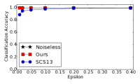
Datasets. We consider three standard benchmark datasets: MNIST444http://yann.lecun.com/exdb/mnist/., Protein555http://osmot.cs.cornell.edu/kddcup/datasets.html., and Forest Covertype666https://archive.ics.uci.edu/ml/datasets/Covertype.. MNIST is a popular dataset used for image classification. MNIST poses a challenge to differential privacy for three reasons: (1) Its number of dimensions is relatively higher than others. To get meaningful test accuracy we thus use Gaussian Random Projection to randomly project to dimensions. This random projection only incurs very small loss in test accuracy, and thus the performance of non-private SGD on dimensions will serve the baseline. (2) MNIST is of medium size and differential privacy is known to be more difficult for medium or small sized datasets. (3) MNIST is a multiclass classification (there are digits), we built “one-vs.-all” multiclass logitstic regression models. This means that we need to construct binary models (one for each digit). Therefore, one needs to split the privacy budget across sub-models. We used the simplest composition theorem [17], and divide the privacy budget evenly.
For Protein dataset, because its test dataset does not have labels, we randomly partition the training set into halves to form train and test datasets. Logistic regression models have very good test accuracy on it. Finally, Forest Covertype is a large dataset with 581012 data points, almost 6 times larger than previous ones. We split it to have 498010 training points and 83002 test points. We use this large dataset for two purposes: First, in this case, one may expect that privacy will follow more easily. We test to what degree this holds for different private algorithms. Second, since training on such large datasets is time consuming, it is desirable to use it to measure runtime overheads of various private algorithms.
Settings of Hyperparameters. The following describes how hyperparameters are set in our experiments. There are three classes of parameters: Loss function parameters, privacy parameters, and parameters for running stochastic gradient descent.
Loss Function Parameters. Given the loss function and regularization parameter , we can derive as described in Section 2. We privately tune in .
Privacy Parameters. are privacy parameters. We vary in for MNIST, and in for Protein and Covertype (as they are binary classification problems and we do not need to divide by 10). is set to be where is the size of the training set size.
SGD Parameters. Now we consider , , and .
Step Size . Step sizes are derived from theoretical analyses of SGD algorithms. In particular the step sizes only depend on the loss function parameters and the time stamp during SGD. Table 4 summarizes step sizes for different settings.
| Non-private | Ours | SCS13 | BST14 | |
|---|---|---|---|---|
| C + -DP | ||||
| C + -DP | Alg. 4 | |||
| SC + -DP | ||||
| SC + -DP | Alg. 5 |
Mini-batch Size . We are not aware of a first-principled way in literature to set mini-batch size (note that convergence proofs hold even for ). In practice mini-batch size typically depends on the system constraints (e.g. number of CPUs) and is set to some number from to . We set in our experiments for fair comparisons with SCS13 and BST14, which shows that our algorithms enjoy both efficiency and substantially better test accuracy.
Note that increasing could reduce noise but makes the gradient step more expensive and might require more passes. In general, a good practice is to set to be reasonably large without hurting performance too much. To assess the impact of this setting further, we include an experiment on varying the batch size in Appendix D. We leave for future work the deeper questions on formally identifying the sweet spot among efficiency, noise, and accuracy.
Number of Passes . For fair comparisons in the experiments below with SCS13 and BST14, for all algorithms tested we privately tune in . However, for our algorithms there is a simpler strategy to set in the strongly convex case. Since our algorithms run vanilla SGD as a black box, one can set a convergence tolerance threshold and set a large as the threshold on the number of passes. Since in the strongly convex case the noise injected in our algorithms (Alg. 2) does not depend on , we can run the vanilla SGD until either the decrease rate of training error is smaller than , or the number of passes reaches , and inject noise at the end.
Note that this strategy does not work for SCS13 or BST14 because in either convex or strongly convex case, their noise injected in each step depends on , so they must have fixed beforehand. Moreover, since they inject noise at each SGD iteration, it is likely that they will run out of the pass threshold.
The above discussion demonstrates an additional advantage of our algorithms using output perturbation: In the strongly convex case the number of passes is oblivious to private SGD.
Radius . Recall that for strongly convex optimization the hypothesis space needs to a have bounded norm (due to the use of regularization). We adopt the practices in [35] and set .
Experimental Environment. All the experiments were run on a machine with Intel Xeon E5-2680 2.50GHz CPUs (-core) and GB RAM running Ubuntu .
4.4 Runtime Overhead and Scalability
Using output perturbation trivially addresses runtime and scalability concerns. We confirm this experimentally in this section.
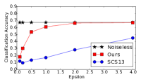
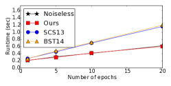
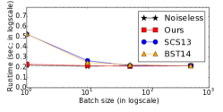
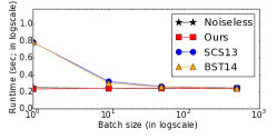
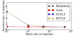
Runtime Overheads. We compare the runtime overheads of our private SGD algorithms against the noiseless version and the other algorithms. The key parameters that affect runtimes are the number of epochs and the batch sizes. Thus, we vary each of these parameters, while fixing the others. The runtimes are the average of warm-cache runs and all datasets fit in the buffer cache of PostgreSQL. The error bars represent confidence intervals. The results are plotted in Figure 5 (a)–(c) and Figure 5 (d)–(f) (only the results of strongly convex, )-differential privacy are reported; the other results are similar and thus, we skip them here for brevity).
The first observation is that our algorithm incurs virtually no runtime overhead over noiseless Bismarck, which is as expected because our algorithm only adds noise once at the end of all epochs. In contrast, both SCS13 and BST14 incur significant runtime overheads in all settings and datasets. In terms of runtime performance for epochs and a batch size of , both SCS13 and BST14 are between 2X and 3X slower than our algorithm. The gap grows larger as the batch size is reduced: for a batch size of and epoch, both SCS13 and BST14 are up to 6X slower than our algorithm. This is expected since these algorithms invoke expensive random sampling code from sophisticated distributions for each mini-batch. When the batch size is increased to , the runtime gap between these algorithms practically disappears as the random sampling code is invoked much less often. Overall, we find that our algorithms can be significantly faster than the alternatives.
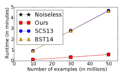
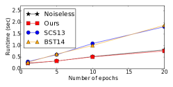
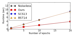
Scalability. We compare the runtimes of all the private SGD algorithms as the datasets are scaled up in size (number of examples). For this experiment, we use the data synthesizer available in Bismarck for binary classification. We produce two sets of datasets for scalability: in-memory and disk-based (dataset does not fit in memory). The results for both are presented in Figure 2. We observe linear increase in runtimes for all the algorithms compared in both settings. As expected, when the dataset fits in memory, SCS13 and BST14 are much slower and in particular the runtime overhead increases linearly as data size grows. This is primarily because CPU costs dominate the runtime. Recall that these algorithms add noise to each mini-batch, which makes them computationally more expensive. We also see that all runtimes scale linearly with the dataset size even in the disk-based setting. An interesting difference is that I/O costs, which are the same for all the algorithms compared, dominate the runtime in Figure 2(b). Overall, these results demonstrate a key benefit of integrating our private SGD algorithm into an RDBMS-based toolkit like Bismarck: scalability to larger-than-memory data comes for free.
 |
 |
4.5 Accuracy and Effects of Parameters

Finally, we report test accuracy and analyze the parameters.
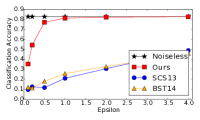
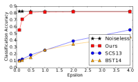
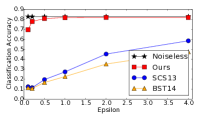
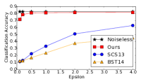
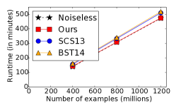
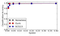
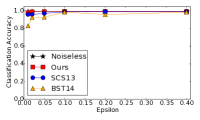
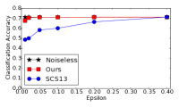
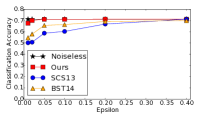
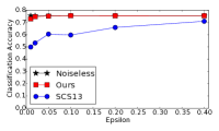
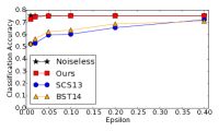
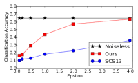
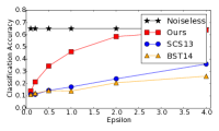
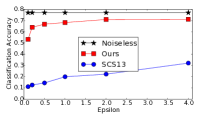
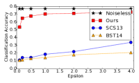
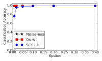
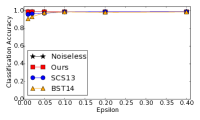
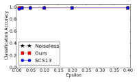
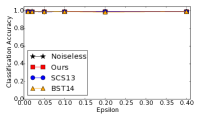
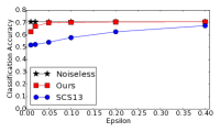
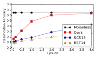
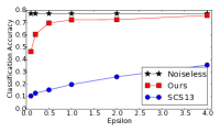
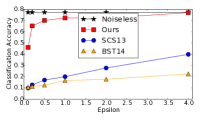
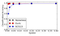
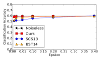
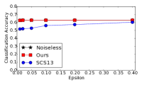
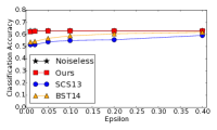
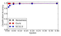
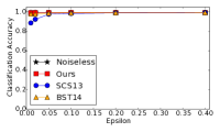
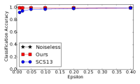
Test Accuracy using Public Data. Figure 3 reports the test accuracy results if one can tune parameters using public data. For all tests our algorithms give significantly better accuracy, up to 4X better than SCS13 and BST14. Besides better absolute performance, we note that our algorithms are more stable in the sense that it converges more quickly to noiseless performance (at smaller ).
Test Accuracy using a Private Tuning Algorithm. Figure 6 gives the test accuracy results of MNIST, Protein and Covertype for all 4 test scenarios using a private tuning algorithm (Algorithm 3). For all tests we see that our algorithms give significantly better accuracy, up to 3.5X better than BST14 and up to 3X better than SCS13.
SCS13 and BST14 exhibit much better accuracy on Protein than on MNIST, since logistic regression fits well to the problem. Specifically, BST14 has very close accuracy as our algorithms, though our algorithms still consistently outperform BST14. The accuracy of SCS13 decreases significantly with smaller .
For Covertype, even on this large dataset, SCS13 and BST14 give much worse accuracy compared to ours. The accuracy of our algorithms is close to the baseline at around . The accuracy of SCS13 and BST14 slowly improves with more passes over the data. Specifically, the accuracy of BST14 approaches the baseline only after .
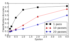
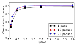
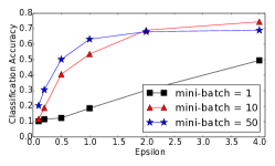
Number of Passes (Epochs). In the case of convex optimization, more passes through the data indicates larger noise magnitude according to our theory results. This translates empirically to worse test accuracy as we perform more passes. Figure 4 (a) reports test accuracy in the convex case as we run our algorithm pass, passes and passes through the MNIST data. The accuracy drops from 0.71 to 0.45 for . One should contrast this with results reported in Figure 4 (b) where doing more passes actually improves the test accuracy. This is because in the strongly convex case more passes will not introduce more noise for privacy while it can potentially improve the convergence.
Mini-batch Sizes. We find that slightly enlarging the mini-batch size can effectively reduce the noise and thus allow the private algorithm to run more passes in the convex setting. This is useful since it is very common in practice to adopt a mini-batch size at around 10 to 50. To illustrate the effect of mini-batch size we consider the same test as we did above for measuring the effect of number of passes: We run Test 1 with passes through the data, but vary mini-batch sizes in . Figure 4 (c) reports the test accuracy for this experiment: As soon as we increase mini-batch size to the test accuracy already improves drastically from 0.45 to 0.71.
4.6 Lessons from Our Experiments
The experimental results demonstrate that our private SGD algorithms produce much more accurate models than prior work. Perhaps more importantly, our algorithms are also more stable with small privacy budgets, which is important for practical applications.
Our algorithms are also easier to tune in practice than SCS13 and BST14. In particular, the only parameters that one needs to tune for our algorithms are mini-batch size and regularization parameter ; other parameters can either be derived from the loss function or can be fixed based on our theoretical analysis. In contrast, SCS13 and BST14 require more attention to the number of passes . For , we recommend setting it as a value between and , noting that too large a value may make gradient steps more expensive and might require more passes. For , we recommend using private parameter tuning with candidates chosen from a typical range of (e.g., choose ).
From the larger perspective of building differentially private analytics systems, however, we note that this paper addresses how to answer one “query” privately and effectively; in some applications, one might want to answer multiple such queries. Studying tradeoffs such as how to split the privacy budget across multiple queries is largely orthogonal to our paper’s focus although they are certainly important. Our work can be plugged into existing frameworks that attempt to address this requirement. That said, we think there is still a large gap between theory and practice for differentially private analytics systems.
5 Related Work
There has been much prior work on differentially private convex optimization. There are three main styles of algorithms – output perturbation [10, 13, 24, 33], objective perturbation [13, 27] and online algorithms [10, 15, 24, 35]. Output perturbation works by finding the exact convex minimizer and then adding noise to it, while objective perturbation exactly solves a randomly perturbed optimization problem. Unfortunately, the privacy guarantees provided by both styles often assume that the exact convex minimizer can be found, which usually does not hold in practice.
There are also a number of online approaches. [24] provides an online algorithm for strongly convex optimization based on a proximal algorithm (e.g. Parikh and Boyd [30]), which is harder to implement than SGD. They also provide an offline version (Algorithm 6) for the strongly convex case that is similar to our approach. SGD-style algorithms were provided by [10, 15, 24, 35]. There has also been a recent work on deep learning (non-convex optimization) with differential privacy [9]. Unfortunately, no convergence result is known for private non-convex optimization, and they also can only guarantee -differential privacy due to the use of advanced composition of -differential privacy.
Finally, our results are not directly comparable with systems such as RAPPOR [18]. In particular, RAPPOR assumes a different privacy model (local differential privacy) where there is no trusted centralized agency who can compute on the entire raw dataset.
6 Conclusion and Future Work
Scalable and differentially private convex ERM have each received significant attention in the past decade. Unfortunately, little previous work has examined the private ERM problem in scalable systems such as in-RDBMS analytics systems. This paper takes a step to bridge this gap. There are many intriguing future directions to pursue. We need to better understand the convergence behavior of private SGD when only a constant number of passes can be afforded. BST14 [10] provides a convergence bound for private SGD when passes are made. SCS13 [35] does not provide a convergence proof; however, the work of [15], which considers local differential privacy, a privacy model where data providers do not even trust the data collector, can be used to conclude convergence for SCS13, though at a very slow rate. Finally, while our method converges very well in practice with multiple passes, we can only prove convergence with one pass. Can we prove convergence bounds of our algorithms for multiple-passes and match the bounds of BST14?
References
- [1] Apache Mahout. mahout.apache.org.
- [2] Apache Spark. https://en.wikipedia.org/wiki/Apache_Spark.
- [3] Grid Search. http://scikit-learn.org/stable/modules/grid_search.html.
- [4] Hinge Loss and Smoothed Variants. https://en.wikipedia.org/wiki/Hinge_loss.
- [5] How many secrets do you have? https://github.com/frankmcsherry/blog/blob/master/posts/2017-02-08.md.
- [6] Preprocessing data in machine learning. http://scikit-learn.org/stable/modules/preprocessing.html.
- [7] Random Projection. https://en.wikipedia.org/wiki/Random_projection.
- [8] random unit vector in multi-dimensional space. http://stackoverflow.com/questions/6283080/random-unit-vector-in-multi-dimensional-space.
- [9] M. Abadi, A. Chu, I. J. Goodfellow, H. B. McMahan, I. Mironov, K. Talwar, and L. Zhang. Deep learning with differential privacy. In Proceedings of the 2016 ACM SIGSAC Conference on Computer and Communications Security, Vienna, Austria, October 24-28, 2016, pages 308–318, 2016.
- [10] R. Bassily, A. Smith, and A. Thakurta. Private empirical risk minimization: Efficient algorithms and tight error bounds. In FOCS, 2014.
- [11] S. Boyd and L. Vandenberghe. Convex Optimization. Cambridge University Press, New York, NY, USA, 2004.
- [12] S. Bubeck. Convex optimization: Algorithms and complexity. Foundations and Trends in Machine Learning, 8(3-4):231–357, 2015.
- [13] K. Chaudhuri, C. Monteleoni, and A. D. Sarwate. Differentially private empirical risk minimization. Journal of Machine Learning Research, 12:1069–1109, 2011.
- [14] K. Chaudhuri and S. A. Vinterbo. A stability-based validation procedure for differentially private machine learning. In NIPS, 2013.
- [15] J. C. Duchi, M. I. Jordan, and M. J. Wainwright. Local privacy and statistical minimax rates. In FOCS, 2013.
- [16] C. Dwork, F. McSherry, K. Nissim, and A. Smith. Calibrating noise to sensitivity in private data analysis. In TCC, 2006.
- [17] C. Dwork and A. Roth. The algorithmic foundations of differential privacy. Foundations and Trends in Theoretical Computer Science, 9(3-4):211–407, 2014.
- [18] Ú. Erlingsson, V. Pihur, and A. Korolova. RAPPOR: randomized aggregatable privacy-preserving ordinal response. In Proceedings of the 2014 ACM SIGSAC Conference on Computer and Communications Security, Scottsdale, AZ, USA, November 3-7, 2014, pages 1054–1067, 2014.
- [19] X. Feng, A. Kumar, B. Recht, and C. Ré. Towards a unified architecture for in-rdbms analytics. In SIGMOD, 2012.
- [20] J. Gray et al. Data Cube: A Relational Aggregation Operator Generalizing Group-By, Cross-Tab, and Sub-Totals. Data Min. Knowl. Discov., 1(1):29–53, Jan. 1997.
- [21] M. Hardt, B. Recht, and Y. Singer. Train faster, generalize better: Stability of stochastic gradient descent. ArXiv e-prints, Sept. 2015.
- [22] M. Hay, A. Machanavajjhala, G. Miklau, Y. Chen, and D. Zhang. Principled evaluation of differentially private algorithms using dpbench. CoRR, abs/1512.04817, 2015.
- [23] J. Hellerstein et al. The MADlib Analytics Library or MAD Skills, the SQL. In VLDB, 2012.
- [24] P. Jain, P. Kothari, and A. Thakurta. Differentially private online learning. In COLT, 2012.
- [25] P. Jain and A. Thakurta. Differentially private learning with kernels. In ICML, 2013.
- [26] R. Johnson and T. Zhang. Accelerating stochastic gradient descent using predictive variance reduction. In NIPS, 2013.
- [27] D. Kifer, A. D. Smith, and A. Thakurta. Private convex optimization for empirical risk minimization with applications to high-dimensional regression. In COLT, 2012.
- [28] A. Nemirovsky and D. Yudin. Problem complexity and method efficiency in optimization. 1983.
- [29] Y. Nesterov. Introductory lectures on convex optimization : a basic course. Applied optimization. Kluwer Academic Publ., 2004.
- [30] N. Parikh and S. P. Boyd. Proximal algorithms. Foundations and Trends in Optimization, 1(3):127–239, 2014.
- [31] B. T. Polyak. Introduction to optimization. Optimization Software, 1987.
- [32] N. L. Roux, M. W. Schmidt, and F. R. Bach. A stochastic gradient method with an exponential convergence rate for finite training sets. In NIPS, 2012.
- [33] B. I. P. Rubinstein, P. L. Bartlett, L. Huang, and N. Taft. Learning in a large function space: Privacy-preserving mechanisms for SVM learning. CoRR, abs/0911.5708, 2009.
- [34] O. Shamir. Without-Replacement Sampling for Stochastic Gradient Methods: Convergence Results and Application to Distributed Optimization. ArXiv e-prints, Mar. 2016.
- [35] S. Song, K. Chaudhuri, and A. D. Sarwate. Stochastic gradient descent with differentially private updates. In GlobalSIP, 2013.
- [36] J. Zhang, X. Xiao, Y. Yang, Z. Zhang, and M. Winslett. Privgene: differentially private model fitting using genetic algorithms. In SIGMOD, 2013.
- [37] J. Zhang, Z. Zhang, X. Xiao, Y. Yang, and M. Winslett. Functional mechanism: Regression analysis under differential privacy. PVLDB, 2012.
- [38] M. Zinkevich. Online convex programming and generalized infinitesimal gradient ascent. In ICML, 2003.
Appendix A Proofs
A.1 Proof of Lemma 6
A.2 Proof of Corollary 2
Proof.
We have that
Therefore
as desired. ∎
A.3 Proof of Lemma 7
Proof.
Let , so we have in total updates. We have the following recursion
| (9) |
This is because at each pass different gradient update operators are encountered only at position (corresponding to the time step ), and so the two inequalities directly follow from the growth recursion lemma (Lemma 4). Therefore, the contribution of the differing entry in the first pass contributes , and generalizing this, the differing entry in the -th pass contributes . Summing up gives the first claimed bound.
For sensitivity, we note that for , the -th pass can only contribute at most to . Summing up gives the desired result. ∎
A.4 Proof of Lemma 8
Proof.
From the Growth Recursion Lemma (Lemma 4) we know that in the -strongly convex case, with appropriate step size, in each iteration either we have a contraction of , or, we have a contraction of plus an additional additive term. In PSGD, in each pass the differing data point will only be encountered once, introducing an additive term, and is contracted afterwards.
Formally, let be the number of updates, the differing data point is at location . Let be the expansion factor at iteration . Then the first pass contributes to , the second pass contributes to . In general pass contributes to .
Let be the contribution of pass to . We now figure out and . Consider , we consider two cases. If , then , and so is expansive. Thus if then before the gap is and after we can apply expansiveness such that
The remaining case is when . In this case we first have -expansiveness due to convexity that the step size is bounded by . Moreover we have -expansiveness for when . Thus
Therefore . Finally, for ,
Summing up gives the desired result. ∎
A.5 Proof of Theorem 8
Proof.
The proof follows exactly the same argument as Theorem 1 of Zinkevich [38], except we change the step size in the final accumulation of errors. ∎
A.6 Proof of Theorem 10
Proof.

Appendix B Results with Huber SVM
In this section we report results on Huber SVM. The standard SVM uses the hinge loss function, defined by , where is the feature vector and is the classification label. However, hinge loss is not differentiable and so our results do not directly apply. Fortunately, it is possible to replace hinge loss with a differentiable and smooth approximation, and it works pretty well either in theory or in practice. Let , we use the following definition from [13],
In this case one can show that (under the condition that all point are normalized to unit sphere) and for , and our results thus apply.
Similar to the experiments with logistic regression, we use standard Huber SVM for the convex case, and Huber SVM regularized by regularizer for the strongly convex case. Figure 7 reports the accuracy results in the case of tuning with a private tuning algorithm. Similar to the accuracy results on logistic regression results, in all test cases our algorithms produce significantly more accurate models. In particular for MNIST our accuracy is up to 6X better than BST14 and 2.5X better than SCS13.
Appendix C Test Accuracy Results on Additional Datasets
In this section we report test accuracy results on additional datasets: HIGGS777https://archive.ics.uci.edu/ml/datasets/HIGGS., and KDDCup-99888https://kdd.ics.uci.edu/databases/kddcup99/kddcup99.html.. The test accuracy results of logistic regression are reported in Figure 8 for tuning with public data, and in Figure 9 for private tuning. These results further illustrate the advantages of our algorithms: For large datasets differential privacy comes for free with our algorithms. In particular, HIGGS is a very large dataset with training points, and this large reduces the noise to negligible for our algorithms, where we achieve almost the same accuracy as noiseless algorithms. However, the test accuracy of SCS13 and BST14 are still notably worse than that of the noiseless version, especially for small . We find similar results for Huber SVM.
Appendix D Accuracy vs. Mini-batch Size
In Figure 10 we report more experimental results when we increase mini-batch size from to . Specifically we test for four mini-batch sizes, . We report the test accuracy on MNIST using the strongly convex optimization, and similar results hold for other optimization and datasets. Encouragingly, we achieve almost native accuracy as we increase the mini-batch size. On the other hand, while the accuracy also increases for SCS13 and BST14 for larger mini-batch sizes, their accuracy is still significantly worse than our algorithms and noiseless algorithms.
Appendix E Sampling Laplace Noise
We discuss briefly how to sample from (3). We are given dimension , -sensitivity and privacy parameter . In the first step, we sample a uniform vector in the unit ball, say (this can be done, for example, by a trick described in [8]). In the second step we sample a magnitude from Gamma distribution , which can be done, for example, via standard Python API (np.random.gamma). Finally we output . The same algorithm is used in [13].