Regression-based reduced-order models to predict transient thermal output for enhanced geothermal systems

Abstract

Reduced-order modeling is a promising approach, as many phenomena can be described by a few parameters/mechanisms. An advantage and attractive aspect of a reduced-order model is that it is computational inexpensive to evaluate when compared to running a high-fidelity numerical simulation. A reduced-order model takes couple of seconds to run on a laptop while a high-fidelity simulation may take couple of hours to run on a high-performance computing cluster. The goal of this paper is to assess the utility of regression-based Reduced-Order Models (ROMs) developed from high-fidelity numerical simulations for predicting transient thermal power output for an enhanced geothermal reservoir while explicitly accounting for uncertainties in the subsurface system and site-specific details. Numerical simulations are performed based on equally spaced values in the specified range of model parameters. Key sensitive parameters are then identified from these simulations, which are fracture zone permeability, well/skin factor, bottom hole pressure, and injection flow rate. We found the fracture zone permeability to be the most sensitive parameter. The fracture zone permeability along with time, are used to build regression-based ROMs for the thermal power output. The ROMs are trained and validated using detailed physics-based numerical simulations. Finally, predictions from the ROMs are then compared with field data. We propose three different ROMs with different levels of model parsimony, each describing key and essential features of the power production curves. The coefficients in proposed regression-based ROMs are developed by minimizing a non-linear least-squares misfit function using Levenberg-Marquardt algorithm. The misfit function is based on the difference between numerical simulation data and reduced-order model. ROM-1 is constructed based on polynomials upto fourth order. ROM-1 is able to accurately reproduce the power output of numerical simulations for low values of permeabilities and certain features of the field-scale data. ROM-2 is a model with more analytical functions consisting of polynomials upto order eight, exponential functions and smooth approximations of Heaviside functions, and accurately describes the field-data. At higher permeabilities, ROM-2 reproduces numerical results better than ROM-1, however, there is a considerable deviation from numerical results at low fracture zone permeabilities. ROM-3 consists of polynomials upto order ten, and is developed by taking the best aspects of ROM-1 and ROM-2. ROM-1 is relatively parsimonious than ROM-2 and ROM-3, while ROM-2 overfits the data. ROM-3 on the other hand, provides a middle ground for model parsimony. Based on $\mathrm{R}^{2}$-values for training, validation, and prediction data sets we found that ROM-3 is better model than ROM-2 and ROM-1. For predicting thermal drawdown in EGS applications, where high fracture zone permeabilities (typically greater than $10^{-15}\,\mathrm{m}^{2}$) are desired, ROM-2 and ROM-3 outperform ROM-1. As per computational time, all the ROMs are $10^{4}$ times faster when compared to running a high-fidelity numerical simulation. This makes the proposed regression-based ROMs attractive for real-time EGS applications because they are fast and provide reasonably good predictions for thermal power output.

Keywords: Enhanced Geothermal Systems (EGS), Reduced-Order Models (ROMs), thermal drawdown, regression.

1. INTRODUCTION AND PROBLEM DESCRIPTION

Enhanced Geothermal Systems (EGS) present a significant and long-term opportunity for widespread power production from new geothermal sources. EGS makes it possible to tap otherwise inaccessible thermal resources in areas that lack traditional geothermal systems. It is estimated that within the USA alone the electricity production potential of EGS is in excess of 100GW. Hence, the efforts to model and predict the performance of EGS reservoirs under various reservoir conditions (such as formation permeability, reservoir temperature, existing fracture/fault connectivity, and in-situ stress distribution) are vital. In this paper, we present a study based on reduced-order modeling using data from the historic Fenton Hill Hot Dry Rock (HDR) project [1]. From a practical point of view, we are interested in developing fast models to examine the potential for supplying thermal energy at sustained rates for commercial operations.

Most of the existing studies related to EGS [2, 3, 4, 5, 6, 7, 8, 9, 10, 11, 12, 13, 14, 15, 16, 17, 18] are based on high-fidelity numerical simulations. These simulations are performed to gain detailed understanding of the physical processes taking place in EGS reservoirs. However, such detailed numerical simulations are computationally expensive as they take hours to run on hundreds of processors, making them prohibitive for real-time applications. Herein, we shall take a different route to model and understand EGS systems based on reduced-order modeling. Reduced-order models are similar to analytical solutions. A major advantage of ROMs are that they take couple of seconds to run on a laptop as compared to high-fidelity numerical simulations. This makes them attractive for real-time and commercial applications. But the procedure to construct ROMs is different compared to constructing analytical solutions. In literature, they are various ways to develop reduced-order models [19, 20, 21, 22, 23, 24]. In our case, reduced-order models are developed and trained based on high-fidelity numerical simulations. ROMs developed from high-fidelity numerical simulation data are not actual reduction of the physical system but are proxy/surrogate models for certain quantities of interest such as thermal power production. As a result, there are no governing equations for such reduced-order models. In the following subsections, we briefly describe the field experiment and need for reduced-order models.

1.1. A brief description of the problem and field experiment

The aim of this paper is to predict the thermal power output during the Long-Term Flow Test (LTFT) experiment of Phase II reservoir at the Fenton Hill HDR test site, located near Los Alamos, New Mexico [25, 26, 27, 28]. This Phase II reservoir was designed to test the HDR concept at temperatures and thermal production rates near those required for a commercial electrical power plant [29, 1]. One of the objectives of the current study is to include site-specific conditions in developing models.

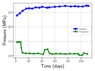
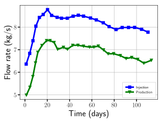
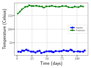
The operation of LTFT experiment at Fenton Hill lasted for 39 months with 11 months of active circulation through the reservoir. The Phase II reservoir comprised of a single injection well and single production well. The injection pressure was in the range of 25 MPa to 30 MPa and production backpressure ranged from 8 MPa to 13 MPa. The injection and production mass flow rates ranged from 7.5 $\mathrm{kg}\,\mathrm{s}^{-1}$ to 8.5 $\mathrm{kg}\,\mathrm{s}^{-1}$ and 5.5 $\mathrm{kg}\,\mathrm{s}^{-1}$ to 7.0 $\mathrm{kg}\,\mathrm{s}^{-1}$. The injection and production temperatures at the well-head ranged from 293 K ($20^{\mathrm{o}}\,\mathrm{C}$) to 303 K ($30^{\mathrm{o}}\,\mathrm{C}$) and 438 K ($165^{\mathrm{o}}\,\mathrm{C}$) to 458 K ($185^{\mathrm{o}}\,\mathrm{C}$). Correspondingly, the bottomhole temperatures at the production well accounting for friction loss are between 453 K ($180^{\mathrm{o}}\,\mathrm{C}$) and 498 K ($225^{\mathrm{o}}\,\mathrm{C}$). For more details on these data sets and other aspects (such as tracer data, microseismic data, fracture networks, fracture connectivity, injection and production wells entry points, and reactive-transport data), see References [29, 1].

1.2. Need for reduced-order models

In recent years, model reduction techniques have proven to be powerful tools for solving various problems in geosciences. In reservoir management and decision-making, ROMs are considered efficient yet powerful techniques to address computational challenges associated with managing realistic reservoirs [30]. Examples of some popular research and scientific endeavors on reduced-order modeling within the context of subsurface processes include Cardoso et al. [19, 20], He et al. [21], Pau et al. [22], and Pasetto et al. [23]. Loosely speaking, the problem of model reduction is to replace a detailed physics-based model of a complex system (or a set of processes) by a much “simpler” and more computationally efficient model than the original model while still accurately predicting those aspects of the system that are of interest. There are several reasons ROMs are useful in the context of EGS, including:

• ROMs facilitate in developing site-specific models which are fast to compute. In general, they can be also used as a substitute model for parameter estimation instead of inverse modeling, which may require repeated evaluation of forward models.

• ROMs can be used as numerical surrogates to perform detailed sensitivity analysis and parametric studies, thereby reducing the overall computational burden of high-fidelity numerical simulations.

• In many-query applications such as EGS, a simple, efficient and predictive model is required for field use. Such a model can greatly reduce (or minimize) the associated operational costs, thereby maximizing the EGS power output potential.

The ROMs developed in this paper are based on regression. They are a combination of polynomials of different degrees, sinusoidal function, exponential function, and logistic function. The coefficients of these polynomials and functions are obtained by training the ROMs on high-fidelity numerical simulation data.

1.3. Objectives and outline of the paper

Among the various potential outputs of interest from a full-physics based simulation for the challenge problem is the thermal power produced. The objective of the study is to develop ROMs for an EGS to predict thermal power output. We are interested in developing a fast and predictive ROM for thermal power output that accurately reproduces detailed simulations. To achieve this, the overall approach involves obtaining thermal power data from detailed physics-based 3D numerical simulations using the parallel subsurface flow simulator PFLOTRAN [31]. Approximate range of model input parameters are constructed based an educated guess of the fractured EGS system (see Kelkar et al. [29, Section-3]). We use equally spaced values of the input parameters to generate power data for several cases. The ROMs are constructed, trained and validated against PFLOTRAN numerical simulations. These ROMs are then used to predict thermal power output and compared with a field thermal power data set from LTFT Fenton Hill HDR Phase II experiment.

The paper is organized as follows: Section 2 describes the physics-based conceptual model, which approximately models the Fenton Hill HDR Phase II reservoir. It also provides a brief overview of the governing equations for fluid flow, thermal drawdown, and numerical methodology to solve the coupled conservation equations. Assumptions in modeling these systems are also outlined. In Section 2, we also perform calibration of the material parameters using the field thermal output data. These values serve as base case for the parameters. Using a range of values around these base case values, sensitiviy analysis is performed using PFLOTRAN and is shown in Section 2. Workflow for ROM development is also described in this section as well. Section 3 details a procedure to construct ROMs for thermal power output. Details of training and validation are provided in this section as well. Predictive capabilities of ROMs with respect to thermal power output and comparison against field-data is also discussed. Finally, conclusions are drawn in Section 4.

2. CONCEPTUAL MODEL, GOVERNING EQUATIONS, AND NUMERICAL METHODOLOGY

In this section, we briefly describe the detailed numerical simulations we used in the development of the ROMs, including those governing equations needed to model physical processes involved in heat extraction within a jointed reservoir. We then present a physics-based conceptual model for an EGS reservoir and corresponding boundary conditions. Finally, we describe a numerical methodology to solve the system of coupled partial differential equations using the subsurface simulator PFLOTRAN. PFLOTRAN solves a system of nonlinear partial differential equations describing multiphase, multicomponent, and multiscale reactive flow and transport in porous materials using finite volume method. Here, we shall restrict to solving the governing equations resulting for single phase fluid (water) flow and heat transfer processes.

2.1. Governing equations: Fluid flow and heat transfer

In order to predict the heat extraction process, we solve the following set of governing equations. This includes balance of mass and balance of energy for fluid flow and thermal drawdown. The governing mass conservation equation for single phase saturated flow is given by:

$$\frac{\partial\varphi\rho}{\partial t}+\mathrm{div}[\rho\mathbf{q}]=Q_{w}$$ (2.1)

where $\varphi$ is the porosity, $\rho$ is the fluid density $[\mathrm{kmol}\,\mathrm{m}^{-3}]$, $\mathbf{q}$ is the Darcy’s flux $[\mathrm{m}\,\mathrm{s}^{-1}]$, and $Q_{w}$ is the volumetric source/sink term $[\mathrm{kmol}\,\mathrm{m}^{-3}\,\mathrm{s}^{-1}]$. The Darcy’s flux is given as follows:

$$\mathbf{q}=-\frac{k}{\mu}\mathrm{grad}[P-\rho gz]$$ (2.2)

where $k$ is the intrinsic permeability $[\mathrm{m}^{2}]$, $\mu$ is the dynamic viscosity $[\mathrm{Pa}\,\mathrm{s}]$, $P$ is the pressure $[\mathrm{Pa}]$, $g$ is the gravity $[\mathrm{m}\,\mathrm{s}^{-2}]$, and $z$ is the vertical component of the position vector $[\mathrm{m}]$. The source/sink term is given as follows:

$$Q_{w}=\frac{q_{M}}{W_{w}}\delta\left(\mathbf{x}-\mathbf{x}_{{\text{\tiny{ss}}}}\right),\quad\mathrm{where}\;\;q_{M}=\frac{\Gamma_{\text{\tiny{well}}}\rho}{\mu}\left(P-P_{\text{\tiny{bhp}}}\right)$$ (2.3)

where $q_{M}$ is the mass flow rate $[\mathrm{kg}\,\mathrm{m}^{-3}\,\mathrm{s}^{-1}]$, $W_{w}$ is the formula weight of water $[\mathrm{kg}\,\mathrm{kmol}^{-1}]$, $\Gamma_{\text{\tiny{well}}}$ denotes the skin/well factor (which regulates the mass flow rate in the production well) [unit-less], $\mathbf{x}_{{\text{\tiny{ss}}}}$ denotes the location of the source/sink, $P_{\text{\tiny{bhp}}}$ is the bottom hole pressure of the production well, and $\delta(\bullet)$ denotes the Dirac delta distribution [32]. The governing equation for energy conservation to model thermal drawdown and corresponding heat extraction processes is given as follows:

$$\frac{\partial}{\partial t}\left(\varphi\rho U+\left(1-\varphi\right)\rho_{\text{\tiny{rock}}}c_{\text{\tiny{p,rock}}}T\right)+\mathrm{div}[\rho\mathbf{q}H-\kappa\mathrm{grad}[T]]=Q_{e}$$ (2.4)

where $U$ is the internal energy of the fluid, $\rho_{\text{\tiny{rock}}}$ is the true density of the rock (or rock grain density), $c_{\text{\tiny{p,rock}}}$ is the true heat capacity of the rock (or rock grain heat capacity), $T$ is the temperature of the fluid, $H$ is the enthalpy of the fluid, $\kappa$ is the thermal conductivity of porous rock, and $Q_{e}$ is the source/sink term for heat extraction.

2.2. Physics-based conceptual model: EGS reservoir

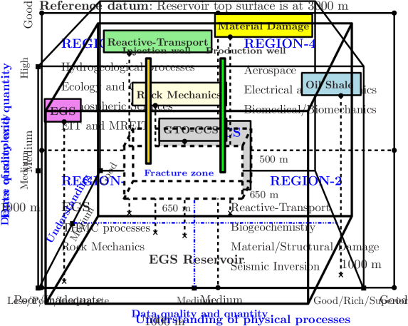
We shall briefly describe the physics-based conceptual model used in the numerical simulation of Phase II Fenton Hill HDR reservoir here. It should be noted that this conceptual model is an approximation of a more complex system (see the References by Kelkar et al. [29] and Brown et al. [1] for a detailed description of the reservoir). Such an approximation is performed to understand the essential features and construct a model that is amenable for numerical simulations. Figure 1 provides a pictorial description of the reservoir. The reference datum, which is the reservoir top surface, is approximately located at a depth of $3000\,\mathrm{m}$. The dimensions and volume of the reservoir are taken to be equal to $1000\times 1000\times 1000\,\mathrm{m}^{3}$. The fracture zone is an approximate representation of the region containing joint networks (fracture networks) and low-permeable porous rock, whose dimensions are taken to be around $650\times 650\times 500\,\mathrm{m}^{3}$. The fracture zone starting and ending coordinates are approximately taken to be $(200\,\mathrm{m},200\,\mathrm{m},200\,\mathrm{m})$ and $(850\,\mathrm{m},850\,\mathrm{m},700\,\mathrm{m})$. The injection and production wells are located at around $(575\,\mathrm{m},575\,\mathrm{m},450\,\mathrm{m})$ and $(675\,\mathrm{m},500\,\mathrm{m},625\,\mathrm{m})$. The distance between the wells being 215.06 $\mathrm{m}$. These are idealized as volumetric source/sink terms in performing the numerical simulations. Reservoir and fracture zone porosities are assumed to be equal to 0.0001 and 0.1. The reservoir rock density, rock specific heat capacity, rock thermal conductivity, rock permeability, fluid heat capacity, fluid density, and fluid injection temperature are taken as 2716 $\mathrm{kg}\,\mathrm{m}^{-3}$, 803 $\mathrm{J}\,\mathrm{kg}^{-1}\,\mathrm{K}^{-1}$, 2.546 $\mathrm{W}\,\mathrm{m}^{-1}\,\mathrm{K}^{-1}$, $10^{-18}\,\mathrm{m}^{2}$, 4187 $\mathrm{J}\,\mathrm{kg}^{-1}\mathrm{K}^{-1}$, 950 $\mathrm{kg}\,\mathrm{m}^{-3}$, and 298 $\mathrm{K}$ (Note that the above system and material parameters are taken from the Reference Swenson et al. [8, Table 1]).

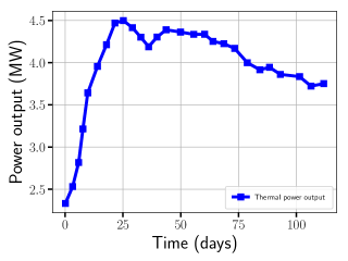
The initial reservoir conditions for the model are at a pressure of 13.2 MPa and temperature of 503 K [29, Section-3]. No flow boundary conditions are assumed for solving the flow equations. Zero gradient boundary conditions are assumed for solving heat transfer equations. Figure 2 shows the respective injection pressure and production backpressure, injection and production mass flow rates, injection and production temperatures, and thermal power extracted during the Phase II LTFT experiment. These field data sets are extracted from the Hot Dry Rock Final Report by Kelkar et al. [29]. To get an estimate of the model parameters for the LTFT set-up, the model is calibrated against field-data. Levenberg-Marquardt (LM) Algorithm implemented in MATK software [33] along with PFLOTRAN is used to estimate the parameters – fracture zone permeability, production temperature, bottom hole pressure, and skin/well factor. By varying the parameters around the calibrated parameter values, sensitivity analysis is performed. Details are discussed in the next subsection.

2.3. Numerical methodology

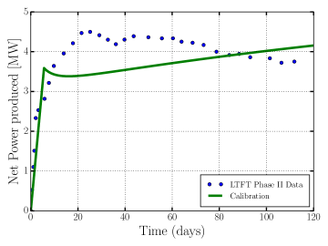
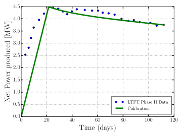
The governing flow and heat transfer equations are solved using the PFLOTRAN simulator, which employs a fully implicit backward Euler for discretizing time and a two-point flux finite volume method for spatial discretization [31, Appendix B]. The resulting non-linear algebraic equations are solved using a Newton-Krylov solver. Numerical simulations are performed for two different scenarios (see Figure 3). Case #1: Calibration is based on constant injection flow rate, which is equal to $7.5\,\mathrm{kg}\,\mathrm{s}^{-1}$ . Case #2: Calibration is performed based on time-varying injection flow rates, whose values are plotted in Figure 2. In this case, the mean square error between thermal power output data based on PFLOTRAN numerical simulations and LTFT field-data is minimized using LM algorithm. The resulting parameters are given as follows:

• Fracture zone permeability

  • Constant injection: $7.75\times 10^{-16}\,\mathrm{m}^{2}$

  • Time-varying injection: $1.78\times 10^{-16}\,\mathrm{m}^{2}$

• Production temperature: $438$ K ($165^{\mathrm{o}}\mathrm{C}$), which is the same for both cases.

• Bottom hole pressure:

  • Constant injection: 9.5 MPa

  • Time-varying injection: 9.42 MPa

• Skin/well factor [unit-less] to regulate mass flow rate in production well:

  • Constant injection: $3.163\times 10^{-13}$

  • Time-varying injection: $5.37\times 10^{-13}$

The power output from the numerical simulation is calculated from the following expression:

Net power produced $$=\left(\textrm{Production mass flow rate}\times\textrm{Fluid heat capacity}\times\textrm{Production temperature}\right)$$

$$-\left(\textrm{Injection mass flow rate}\times\textrm{Fluid heat capacity}\times\textrm{Injection temperature}\right)$$ (2.5)

Figure 3 shows the approximate fit of the PFLOTRAN numerical simulation with the field-scale data of the power output based on the parameters estimated for Case #1 and Case #2. The $\mathrm{R}^{2}$-values for Case #1 and Case #2 are equal to 0.74 and 0.68, which are close to each other. The mean square error (MSE) values for Case #1 and Case #2 are 0.603 and 0.018, which are considerably different. Reason being that the LM algorithm calibrates the model parameters by minimizing the MSE value. It should be noted that the calibrated parameters of the constant injection flow rate case and time-varying injection flow rate case are of the same order, which is enough for performing sensitivity analysis to identify key sensitive input parameters for ROMs construction. The next subsection describes the workflow for ROM construction and the corresponding numerical studies on various model parameters [34].

2.4. Sensitivity analysis, ROM development workflow, and numerical results

In this subsection, we perform sensitivity studies on various input/output model parameters to model EGS reservoirs. Such an analysis is performed to identify key sensitive parameters for ROM inputs. These model parameters include mass flow rate at the injection well, skin/well factor to regulate mass flow rate in production well, fracture zone permeability, and bottom hole pressure.

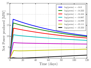
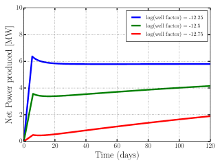
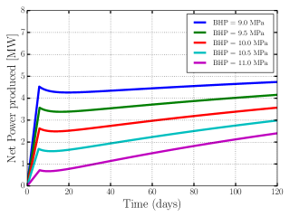
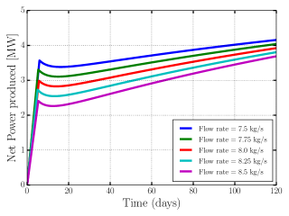
Figure 4 shows the PFLOTRAN numerical simulation results for the above four key parameters. These figures are plotted for each sensitive parameter by keeping all other parameters fixed to base case calibrated values. For example, if fracture zone permeability is varied from the base value (which is equal to $7.75\times 10^{-16}\,\mathrm{m}^{2}$), the other three estimated values for the parameters are kept constant. This is done to show, identify, and rank the key sensitive input parameters for the ROMs. Based on Figure 4, it is apparent that the power production is highly sensitive to varying fracture zone permeability and least sensitive to injection mass flow rates. Correspondingly, the skin/well factor to control mass flow rate in production well and bottom hole pressure (BHP) are second and third in sensitivity ranks after fracture zone permeability. To consolidate, the ranking of importance of inputs for ROM development are given as follows (in the decreasing order):

1. Fracture zone permeability (power production varies in a non-linear fashion)

2. Skin/well factor to regulate mass flow rate in production well

3. Bottom hole pressure

4. Injection mass flow rate (power production varies in a linear fashion)

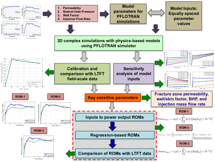
ROM development is summarized as a flowchart in Figure 5. The next section describes an approach to construct ROMs for power output.

3. REDUCED-ORDER MODELING

The objective of model reduction methodologies is to use the knowledge generated by high fidelity and time-consuming numerical simulations to generate special functions that make use of properties of underlying systems, thereby obtaining a good understanding of the phenomena of interest. Subsection 1.2 discusses many reasons why such a detail is warranted. We shall now provide an overview of some popular model order reduction methods and algorithms. These techniques either use physical (or other) insight or sensitivity studies on model parameters as a basis to reduce the complexity of the underlying problem and obtain a good approximation of the required output in an efficient way.

Some popular model reduction methods include regression-based model order reduction [35, 36, 37], operational model order reduction [38, 39], compact reduced-order modeling [38], truncated balanced realization [40], optimal Hankel-norm model order reduction [41], Gaussian process regression (GPR) [42, 22], proper orthogonal decomposition (POD) [43], asymptotic waveform evaluation (AWE) and its variants [44], Pade via Lanczos (PVL) and its variants [45], spectral Lanczos decomposition method (SLDM) [46], and truncation-based model order reduction [38]. For more details on these methods, algorithms, and implementation aspects (see References Qu, [47], Schilders et al. [38], Quarteroni and Rozza [48], and Mignolet et al. [49]). Here, we shall construct reduced-order models based on regression-based model order reduction methods, which result in simple thermal power output ROMs. These ROMs consist of a set of algebraic relations that depend on the key sensitive parameters (which is fracture zone permeability) that can be evaluated very quickly.

3.1. Reduced-order models for power output based on regression-based methods

ROMs are constructed using a combination of polynomials, trigonometric functions, exponential functions, and smooth approximation of step functions. Logistic functions are chosen as the smooth-approximation of step functions. The rationale behind choosing such functions are as follows: Polynomials, trigonometric functions, and exponential functions capture the increase and decay part of the field-scale power output data and PFLOTRAN numerical simulations, while the logistic functions are intended to capture the peaks and sudden variations. The coefficients of these functions are constructed through a non-linear least-squares regression fit to the PFLOTRAN simulations. To obtain the respective coefficients of the functions in the ROMs, non-linear least-squares regression was performed using the optimization solvers available in the open-source Python package Scipy [50].

Below we provide a summary of ROMs construction. It should be noted that all of the simulation data from the sensitivity analysis is used to train and validate the ROMs:

• Training data from PFLOTRAN simulations is used to construct all ROMs. These simulations are performed for log(permeability) values equal to -14.0, -14.444, -14.667, -14.889, and -15.333.

• For ROM-2, in addition to above training datasets, a small subset of field-scale data is used to construct the ROM. These include the LTFT field thermal power data at times $t=0,20,25,40,60,80,100,$ and $120$.

• For validation, the PFLOTRAN simulations performed at log(permeability) values equal to -14.222 and -15.111 are used.

• For prediction, the LTFT thermal power output field data is used.

• ROM-1 is constructed using polynomials of order upto degree four. ROM-2 is constructed using polynomials of order upto degree eight, sine function, exponential function, and smooth approximation of Heaviside functions. ROM-3 is constructed using polynomials of order upto degree ten.

• The coefficients of the ROMs are determined by minimizing the sum of squares of nonlinear functions. This is achieved by using Scipy library’s non-linear least-squares fit function called “scipy.optimize.curve-fit”.

• Using the developed ROMs, the $\mathrm{R}^{2}$-values are then calculated for training, validation, and prediction data.

It should be noted that a small subset of field data is used to train a particular ROM, which is ROM-2. At these values, we exactly reproduce field thermal power output for calibrated permeability value. However, other ROMs are not trained using the observation data. Observation data is first used to obtain realistic parameter range to generate the simulation datasets. These simulation datasets are then used to develop the ROMs. Figure 3 shows the calibration to obtain the base case parameter values for the simulation datasets. The parameters used here include fracture zone permeability, bottom hole pressure, and well factor. Then, based on a sensitivity analysis study, we found the fracture zone permeability to be the most sensitive parameter and so the ROMs were constructed as a function of time and permeability.

Next, we propose and discuss three regression-based reduced-order models with different levels of model parsimony. Algorithm 1 provides a detailed description of the proposed regression-based ROMs construction. Each model has it own pros and cons, which are described below:

3.1.1. Thermal power output ROM-1

$$\textrm{Power}_{\text{\tiny{rom-1}}}=a_{0}(t)+\displaystyle\sum\limits_{i=1}^{3}a_{i}(t)\left(|\mathrm{log}(k_{\text{\tiny{fz}}})|+10^{-6}t\right)^{i}$$ (3.1)

where $t$ denotes the time in days, the coefficients $a_{i}$ are function of time (days), and $k_{\text{\tiny{fz}}}$ is the fracture zone permeability.

3.1.2. Thermal power output ROM-2

$$\textrm{Power}_{\text{\tiny{rom-2}}}=b_{0}(t)+\displaystyle\sum\limits_{i=1}^{3}b_{i}(t)\left(|\mathrm{log}(k_{\text{\tiny{fz}}})|+10^{-6}t\right)^{i}+\underbrace{\displaystyle\sum\limits_{j=1}^{29}m_{j}\left(1+\tanh(n_{j}(t-t_{j}))\right)^{r_{j}}}_{\text{\tiny{Smooth approximation of Heaviside function}}}$$ (3.2)

3.1.3. Thermal power output ROM-3

$$\textrm{Power}_{\text{\tiny{rom-3}}}=c_{0}(t)+\displaystyle\sum\limits_{i=1}^{3}c_{i}(t)\left(|\mathrm{log}(k_{\text{\tiny{fz}}})|+10^{-6}t\right)^{i}$$ (3.3)

Algorithm 1 A numerical methodology to construct regression-based reduced-order models for EGS

1:  INPUTs for PFLOTRAN simulations: Fracture zone permeability, bottom hole pressure, well factor, and injection flow rate.

2:  To construct regression-based ROMs, get high-fidelity numerical simulation data by running PFLOTRAN simulator for different parameter values. Total number of simulations = 2625.

• Logarithm of fracture zone permeability = $-14.0,-14.222,-14.444,-14.667,$
  $-14.889,-15.111,-15.333$.

• Logarithm of well factor = $-12.25,-12.5,-12.75$.

• Bottom hole pressure = $9.0,9.5,10.0,10.5,11.0$.

• Injection mass flow rate = $7.5,7.75,8.0,8.25,8.5$.

3:  Post-process each high-fidelity numerical simulation to obtain thermal power output as function of time. Then, perform sensitivity analysis and identify the dominant parameter. In our case, we found fracture zone permeability is dominant. See Subsection 2.4 for more details.

4:  The proposed regression-based ROMs are function of time and dominant parameter, which is fracture zone permeability. See Equations (3.1)–(3.3).

5:  To construct, train, and validate ROMs, among 2625 high-fidelity simulation dataset we choose a subset with varying fracture zone permeability (while other parameters are kept constant). The values of the other parameters correspond to the calibration case.

• Calibration case parameter values are: Logarithm of well factor = $-12.5$, bottom hole pressure = $9.5$, and injection mass flow rate = $7.5$.

• There are a total of 7 PFLOTRAN simulations that are used in the proposed ROM construction methodology. Out of 7 simulations, 5 simulations are used for training and 2 simulations are used for validation of ROMs. LTFT thermal power output data is used for prediction.

6:  ROM-1 construction: $a_{0}(t)+\displaystyle\sum\limits_{i=1}^{3}a_{i}(t)\left(|\mathrm{log}(k_{\text{\tiny{fz}}})|+10^{-6}t\right)^{i}$

• Polynomials of order upto degree four are selected.

• The coefficients in $a_{i}(t)$ are obtained my minimizing the error between high-fidelity simulation data and the explicit expression of ROM-1.

• The coefficient values, which are obtained by solving the non-linear least-squares regression using Levenberg-Marquardt algorithm are given by Equations (4.1a)–(4.1d).

7:  ROM-2 construction: $b_{0}(t)+\displaystyle\sum\limits_{i=1}^{3}b_{i}(t)\left(|\mathrm{log}(k_{\text{\tiny{fz}}})|+10^{-6}t\right)^{i}+\displaystyle\sum\limits_{j=1}^{29}m_{j}\left(1+\tanh(n_{j}(t-t_{j}))\right)^{r_{j}}$

• Polynomials of order upto degree eight, sine, exponential, and smooth approximation of Heaviside functions are selected.

• The non-linear least-squares regression problem is solved with the constraint that at times $t=0,20,25,40,60,80,100,$ and $120$, the ROM-2 model output matches the LTFT thermal power output data. The coefficients are given by Equations (4.2)–(4.4j).

8:  ROM-3 construction: $a_{0}(t)+\displaystyle\sum\limits_{i=1}^{3}a_{i}(t)\left(|\mathrm{log}(k_{\text{\tiny{fz}}})|+10^{-6}t\right)^{i}$

• Polynomials of order upto degree ten are selected. ROM-3 is constructed in similar fashion to ROM-1. The coefficient values in $c_{i}(t)$ are given by Equations (4.5)–(4.5).

9:  OUTPUTS: Regression models for ROM-1, ROM-2, and ROM-3. Model expressions are given in Appendix. They are used to predict thermal power output.

Table 1. Summary of proposed reduced-order models for thermal power output. A small subset of field-scale data is used to construct the ROM-2. These include the LTFT field thermal power data at times $t=0,20,25,40,60,80,100,$ and $120$.

Model	Thermal Power Output
ROM-1	$a_{0}(t)+\displaystyle\sum\limits_{i=1}^{3}a_{i}(t)\left(|\mathrm{log}(k_{\text{\tiny{fz}}})|+10^{-6}t\right)^{i}$
ROM-2	$b_{0}(t)+\displaystyle\sum\limits_{i=1}^{3}b_{i}(t)\left(|\mathrm{log}(k_{\text{\tiny{fz}}})|+10^{-6}t\right)^{i}+\displaystyle\sum\limits_{j=1}^{29}m_{j}\left(1+\tanh(n_{j}(t-t_{j}))\right)^{r_{j}}$
ROM-3	$c_{0}(t)+\displaystyle\sum\limits_{i=1}^{3}c_{i}(t)\left(|\mathrm{log}(k_{\text{\tiny{fz}}})|+10^{-6}t\right)^{i}$

Table 2. $R^{2}$-values for training, validation, and prediction of numerical simulations and LTFT field-data. Out of total seven simulation datasets, 5 were used for training and 2 for validation. To construct training dataset, numerical simulations are performed for log(permeability) values equal to -14.0, -14.444, -14.667, -14.889, and -15.333. To construct validation dataset, numerical simulations are performed for log(permeability) values of -14.222 and -15.111. Prediction dataset being the LTFT thermal power output field-data.

Model	$R^{2}$-values
	Training	Validation	Prediction
ROM-1	0.489, 0.326, 0.22, 0.75, and 0.96	0.406 and 0.407	0.668
ROM-2	0.877, 0.804, 0.796, 0.689, and 0.573	0.817 and 0.542	0.986
ROM-3	0.917, 0.896, 0.9, 0.889, and 0.813	0.892 and 0.893	0.824

The above ROMs are used to predict LTFT thermal power output data as function of time and fracture zone permeability. As per computational cost, the time taken to run a PFLOTRAN simulation is around 45 seconds. To construct the regression ROMs described above we need 5 high-fidelity simulations for training and 2 high-fidelity simulations for validation. Hence, the total time taken to run 7 high-fidelity simulations is around 315 seconds. To construct ROM-1, ROM-2, and ROM-3, we need to find coefficients of $a_{i}(t)$, $b_{i}(t)$, and $c_{i}(t)$. The coefficients of the ROMs are obtained by minimizing the sum of squares of nonlinear functions with respect to training data using Levenberg-Marquardt algorithm. The procedure to obtain these coefficients is described in Algorithm 1 and the coefficient values are given in Appendix. The Levenberg-Marquardt algorithm takes around 0.06, 0.16, and 0.1 seconds to obtain the coefficients of ROM-1, ROM-2, and ROM-3. The time taken by ROM-1, ROM-2, and ROM-3 to make a prediction is around 0.0002, 0.0015, and 0.0008 seconds. This means the ROMs are $10^{4}$ times faster than a high-fidelity numerical simulation.

Remark 3.1.

The regression-based ROMs are specific to this EGS application. The proposed ROMs can be generalized by removing site-specific aspects in ROMs construction in Algorithm 1. These include, relaxing the range of injection rates, well factor values, bottom hole pressures, and fracture zone permeability. For a new site, first we need to constrain the parameter space specific to that site. Then, we just have to use the same methodology proposed in Algorithm 1 to construct regression-based ROMs specific to the new site.

3.2. Discussion and inferences: Predictive capabilities of ROMs with respect to field-scale data and PFLOTRAN

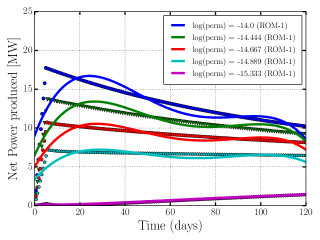
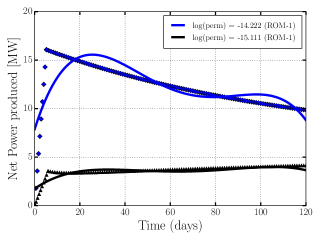
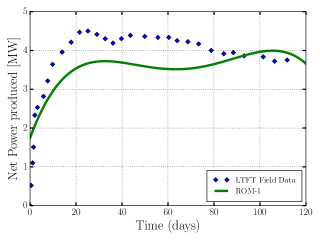
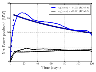
We shall now provide a rationale behind the construction of these ROMs. Moreover, we shall analyze the capabilities of these three ROMs in describing the trends in field-scale data and PFLOTRAN simulations. The construction of ROM-1 is purely based on polynomials. This ROM consists of power-series terms (up to order four) involving natural logarithm of fracture zone permeability and time. The coefficients of the ROM-1 are constructed by matching the power output of PFLOTRAN numerical simulations at certain fixed intervals of time (for various fracture zone permeabilities). Figure 6 shows the training, validation using numerical simulations of ROM-1 along with its predictions. The predictions are compared with field power data. The behavior of ROM-1 is clearly distinct from the PFLOTRAN predictions (i.e., PFLOTRAN predicts a rapid increase in the first few days followed by a smooth decline over the rest of the time period, whereas ROM-1 shows a more gradual rise followed by a varying decline). Nevertheless, for time periods between 20-100 days, ROM-1 is able to accurately reproduce the power output of numerical simulations for low values of fracture zone permeability. However, as the fracture zone permeability increases, there is a considerable deviation between ROM-1 outputs and PFLOTRAN numerical simulations. This is because ROM-1 is constructed by matching PFLOTRAN numerical simulations only at certain time intervals. Moreover, the polynomial order considered to construct the ROM is very low.

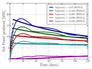
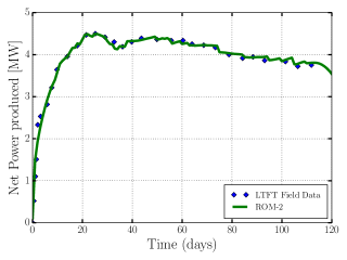
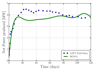
In terms of predicting the field-scale data, ROM-1 is able to reproduce only certain qualitative features of the field-scale data (Figure 6) and is relatively parsimonious. These aspects include the initial increase of power output, the corresponding decrease after the time $t=20$ days, and then an increase in the power output after $t=100$ days. However, quantitatively, the difference in power output values of ROM-1 and LTFT experiment are high. Figure 7 shows the behavior of ROM-2. From equation (3.2), it is evident that ROM-2 has more number of terms and coefficients than ROM-1. The motivation behind the construction of such a model is that we would like to accurately describe the LTFT experiment at various time intervals. ROM-2 is constructed by adding smooth approximations of step functions and higher-order polynomials to ROM-1. Figure 7 shows the training and validation against numerical simulations and final predictions of ROM-2. The predictions are compared with LTFT experiment. From this figure, it evident that ROM-2 shares some of the limitations of ROM-1: It does not reproduce the rapid rise in net power produced for the initial days of operation (albeit the fit is better than ROM-1), nor does it reproduce a nearly linear decline for times out to 120 days. ROM-2 qualitatively reproduces the decline portion of the PFLOTRAN predictions (for days 20-120), but it over predicts the numerical simulations, quantitatively. In general, ROM-2 reproduces the PFLOTRAN results better than ROM-1 at higher permeabilities. Interestingly, power output predicted using ROM-2 closely matches the LTFT experiment, qualitatively and quantitatively. However, ROM-2 is overfitted (see Table 2 for $\mathrm{R}^{2}$-values). In terms of reproducing the field-scale data and PFLOTRAN simulations at higher permeability ROM-2 is certainly better than ROM-1.

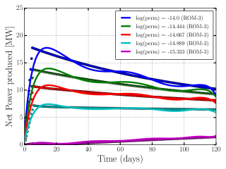
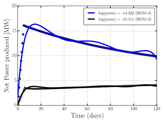
Motivated by these two ROMs, ROM-3 is constructed. The philosophy of ROM-3 is to use only polynomials. The number of terms is determined by the coefficient values. The maximum possible order for the polynomial chosen is 10. This is because as the order of polynomial increases the values of the coefficient are close to machine precision (close to zero). Figure 8 shows the training, validation using numerical simulations of ROM-3 along with its predictions. The predictions are compared with field power data. From this figure (8a/9a), it is apparent that ROM-3 more accurately reproduces the trend in the behavior of thermal power output than ROM-2. For numerical simulations, as the permeability increases the deviations in the output values of ROM-3 and PFLOTRAN numerical simulations are not very large as compared to ROM-1 and ROM-2. In the case of the LTFT experiment, ROM-3 is able to accurately describe the increase in the thermal power output in initial stages. After time $t=20$ days, when compared to the performance of ROM-2, ROM-3 is not exactly a close match to the LTFT data quantitatively. However, qualitatively, ROM-3 is a much better model compared to ROM-1 due to the incorporation of higher-order polynomials (see Tables 1 and 2 for more details). In short, ROM-3 neither overfits nor underfits the LTFT experiment data. Hence, ROM-3 is a better model compared to ROM-2 and ROM-1 and provides a middle ground for model parsimony. The model can be improved by incorporating other input terms such as well factor, bottom hole pressure, and injection mass flow rates. This is beyond the scope of the current paper and will be considered in our future work. Table 1 summarizes the ROMs and their $\mathrm{R}^{2}$-values for training, validation, and prediction of numerical simulations and LTFT field-data.

To conclude the discussion, the following can be inferred based on Figures 6–8 and equations (3.1)–(4.5):

• In reproducing PFLOTRAN numerical simulations, for low values of permeability, ROM-1 outperforms ROM-2 and ROM-3. At higher values of permeability, ROM-2 outperforms ROM-1 and ROM-3. In predicting LTFT data, ROM-2 outperforms ROM-3 and ROM-1. However, ROM-3 is able to describe the initial trend in the field-data and other qualitative aspects (such as the rise in power production after $t=10$ days and decline after $t=30$ days).

• At first glance, it may seem that ROM-2 may be the best model in reproducing LTFT data. However, from Figure 7, it is evident that ROM-2 considerably deviates from the PFLOTRAN simulations at low values of permeability. Typically, for EGS applications, higher effective fracture zone permeabilities are desired [1]. This is because in many practical scenarios (assuming that reservoir matrix permeability to be very low), higher fracture zone permeabilities can be correlated to (possibly) well connected and dispersed discrete fracture networks [51]. This means that the fluid sweeps through a larger fractured volume (as compared to lower fracture zone permeabilities) resulting in higher power production at producing wells. To model such scenarios, we believe ROM-2 and ROM-3 are better models than ROM-1.

4. CONCLUDING REMARKS

In this paper, we have presented various reduced-order models to describe different aspects of the numerical simulations and LTFT field-scale power output data of Phase II Fenton hill geothermal reservoir. First, we described the governing equations for fluid flow in the fractured reservoir and corresponding thermal drawdown. Second, we have presented a physics-based conceptual model for an EGS reservoir. The conceptual model is an approximation of a more complex system, which is used to understand the essential features of the systems and make it amenable for numerical simulations. Field-scale data sets, which are extracted from the documents provided by the geothermal code comparison project, are used to estimate the parameters of the EGS system under consideration. These data sets include pressures, backpressures, mass flow rates, and temperatures at both injection and production sites. Third, sensitivity analysis is performed on these inputs to identify and rank the key parameters: fracture zone permeability, well factor, injection flow rate and bottom hole pressure. Based on this analysis, fracture zone permeability was found to be most important and so we used only permeability and time as the parameters for ROM construction. Finally, the ROMs are developed using the numerical simulations obtained based on equally spaced parametric values.

The ROMs are built (trained and validated) using simulation data from the numerical model (PFLOTRAN) as shown in Figures 6, 7, and 8. Then, these ROMs are used to predict the behavior of an EGS system, specifically, Fenton Hill system. The input to these ROMs are permeability and time. From the calibration in Figure 4, we first obtain the permeability of the Fenton Hill EGS system. This permeability value along with time are then used in ROM predictions, and compared with the observation data to evaluate the performance of the ROMs.

We evaluated three different ROMs with different levels of model parsimony, each describing key and essential features of the LTFT power output data. The first ROM is a simple model and is able to accurately describe the power output at low fracture zone permeabilities, and is relatively parsimonious. The second ROM is a more complex model than ROM-1. However, ROM-2 shares some of the limitations of ROM-1. In general, ROM-2 reproduces the numerical simulations better than ROM-1 at higher permeabilities. The interesting part of ROM-2 is that the power output predicted closely matches the LTFT experiment, qualitatively and quantitatively. The third ROM is constructed by taking the best aspects of ROM-1 and ROM-2, and provides a middle ground for model parsimony. ROM-3 is able to quantitatively and qualitatively describe the trend in the power output at different time levels for both PFLOTRAN numerical simulations and LTFT power output data.

From these ROM development workflows and sensitivity analyses, it is evident that this study has demonstrated that simple reduced-order models are able to capture various complex features in the system. This work provides confidence in developing simple and efficient transient reduced-order models for geothermal field use. For EGS applications, higher fracture zone permeability is desired [1]. This is because at higher permeabilities power output is higher as the fluid sweeps through a larger fracture zone volume. For such scenarios (at higher permeabilities in predicting the thermal power production), ROM-2 and ROM-3 outperform ROM-1. We think ROM-2 and ROM-3 show promise for EGS studies.

APPENDIX

The coefficients for ROM-1 are given as follows:

$$a_{0}(t) =-2.689\times 10^{3}-9.951\times 10^{2}t+28.37t^{2}-3.013\times 10^{-1}t^{3}+1.095\times 10^{-3}t^{4}$$ (4.1a)

$$a_{1}(t) =5.517\times 10^{2}+2.01\times 10^{2}t-5.751t^{2}-6.111\times 10^{-2}t^{3}-2.222\times 10^{-4}t^{4}$$ (4.1b)

$$a_{2}(t) =-3.718\times 10^{1}-1.347\times 10^{1}t+3.867\times 10^{-1}t^{2}-4.112\times 10^{-3}t^{3}+1.495\times 10^{-5}t^{4}$$ (4.1c)

$$a_{3}(t) =8.241\times 10^{3}+2.998\times 10^{-1}t-8.634\times 10^{-3}t^{2}+9.184\times 10^{-5}t^{3}-3.339\times 10^{-7}t^{4}$$ (4.1d)

For ROM-2, the coefficients $b_{i}$ are functions of time (days), which are given as follows:

$$b_{0}(t) =2.318\times 10^{3}-2.466\times 10^{3}t+1.338\times 10^{2}t^{2}-3.413t^{3}+4.612\times 10^{-2}t^{4}$$

$$-3.393\times 10^{-4}t^{5}+1.376\times 10^{-6}t^{6}-3.538\times 10^{-9}t^{7}+6.869\times 10^{-12}t^{8}$$

$$-2.307\times 10^{3}\times(0.1)^{t}+1.342\sin(t)$$ (4.2a)

$$b_{1}(t) =-4.623\times 10^{2}+4.992\times 10^{2}t-2.713\times 10^{1}t^{2}+6.918\times 10^{-1}t^{3}-9.339\times 10^{-3}t^{4}$$

$$+6.856\times 10^{-5}t^{5}-2.766\times 10^{-7}t^{6}+7.056\times 10^{-10}t^{7}-1.369\times 10^{-12}t^{8}$$

$$-2.307\times 10^{3}\times(0.1)^{t}-2.676\sin(t)$$ (4.2b)

$$b_{2}(t) =3.103\times 10^{1}-3.353\times 10^{1}t+1.825t^{2}-4.652\times 10^{-2}t^{3}+6.28\times 10^{-4}t^{6}-4.608\times 10^{-6}t^{5}$$

$$+1.858\times 10^{-8}t^{6}-4.734\times 10^{-11}t^{7}+9.191\times 10^{-14}t^{8}-3.087\times 10^{1}\times(0.1)^{t}$$

$$+1.796\times 10^{-2}\sin(t)$$ (4.2c)

$$b_{3}(t) =-6.997\times 10^{-1}+7.477\times 10^{-1}t-4.073\times 10^{-2}t^{2}+1.038\times 10^{-3}t^{3}-1.402\times 10^{-5}t^{4}$$

$$+1.031\times 10^{-7}t^{5}-4.168\times 10^{-10}t^{6}-1.068\times 10^{-12}t^{7}-2.073\times 10^{-15}t^{8}$$

$$+6.964\times 10^{-1}\times(0.1)^{t}-4.048\times 10^{-4}\sin(t)$$ (4.2d)

The parameters $t_{j}$ (days) are chosen in such a way that the ROM outputs be close to that of the field-scale LTFT thermal power output at the $i$-th time-snapshots/time-levels. These time values are given as follows:

$$t_{1}=10,t_{2}=15,t_{3}=17.5,t_{4}=19,t_{5}=20,t_{6}=21,t_{7}=22.5,t_{8}=25,t_{9}=30,t_{10}=32.5$$ (4.3a)

$$t_{11}=35,t_{12}=37.5,t_{13}=50,t_{14}=52.5,t_{15}=55,t_{16}=60,t_{17}=62.5,t_{18}=65,t_{19}=70,$$ (4.3b)

$$t_{20}=75,t_{21}=80,t_{22}=85,t_{23}=87.5,t_{24}=90,t_{25}=95,t_{26}=100,t_{27}=105,$$ (4.3c)

$$t_{28}=110,t_{29}=112.5$$ (4.3d)

The coefficients $m_{j},n_{j},r_{j}$ are given as follows:

$$m_{1}=0.1,m_{2}=0.085,m_{3}=0.05,m_{4}=-0.0125,m_{5}=0.125,m_{6}=0.1,m_{7}=-0.0125$$ (4.4a)

$$m_{8}=0.085,m_{9}=-0.075,m_{10}=-0.085,m_{11}=0.085,m_{12}=0.125,m_{13}=-0.085,$$ (4.4b)

$$m_{14}=-0.01,m_{15}=-0.05,m_{16}=-0.075,m_{17}=-0.075,m_{18}=-0.025,m_{19}=-0.015,$$ (4.4c)

$$m_{20}=-0.15,m_{21}=-0.05,m_{22}=-0.05,m_{23}=-0.05,m_{24}=-0.15,m_{25}=-0.1,$$ (4.4d)

$$m_{26}=-0.085,m_{27}=-0.175,m_{28}=-0.05,m_{29}=0.05,$$ (4.4e)

$$n_{1}=n_{2}=n_{3}=100,\;n_{4}\;\mathrm{to}\;n_{29}=1000$$ (4.4f)

$$r_{1}=r_{2}=r_{3}=1,r_{4}=0.5,r_{5}=0.25,r_{6}=0.5,r_{7}=0.1,r_{8}=0.25,r_{9}=0.75,r_{10}=0.02$$ (4.4g)

$$r_{11}=0.01,r_{12}=0.01,r_{13}=0.25,r_{14}=1.5,r_{15}=1.75,r_{16}=r_{17}=r_{18}=r_{19}=r_{20}=0.01$$ (4.4h)

$$r_{21}=r_{22}=r_{23}=0.01,r_{24}=0.025,r_{25}=0.075,r_{26}=0.01,r_{27}=0.15,$$ (4.4i)

$$r_{28}=0.01,r_{29}=0.01$$ (4.4j)

For ROM-3, the coefficients $c_{i}$ are functions of time (days), which are given as follows:

$$c_{0}(t) =7.913\times 10^{2}-1.747\times 10^{3}t+2.089\times 10^{1}t^{2}+5.173t^{3}-3.234\times 10^{-1}t^{4}$$

$$+9.397\times 10^{-3}t^{5}-1.613\times 10^{-4}t^{6}+1.727\times 10^{-6}t^{7}-1.134\times 10^{-8}t^{8}$$

$$+4.183\times 10^{-11}t^{9}-6.627\times 10^{-14}t^{10}$$ (4.5a)

$$c_{1}(t) =-1.578\times 10^{2}+3.557\times 10^{2}t-4.613t^{2}-1.093t^{3}+6.432\times 10^{-2}t^{4}$$

$$-1.872\times 10^{-3}t^{5}+3.215\times 10^{-5}t^{6}-3.442\times 10^{-7}t^{7}+2.261\times 10^{-9}t^{8}$$

$$-8.337\times 10^{-12}t^{9}+1.321\times 10^{-14}t^{10}$$ (4.5b)

$$c_{2}(t) =1.059\times 10^{1}-2.391\times 10^{1}t-3.136\times 10^{-1}t^{2}+6.835\times 10^{-2}t^{3}-4.316\times 10^{-3}t^{4}$$

$$+1.256\times 10^{-4}t^{5}-2.158\times 10^{-6}t^{6}+2.311\times 10^{-8}t^{7}-1.517\times 10^{-10}t^{8}$$

$$+5.597\times 10^{-13}t^{9}-8.868\times 10^{-16}t^{10}$$ (4.5c)

$$c_{3}(t) =-2.388\times 10^{-1}+5.305\times 10^{-1}t-6.637\times 10^{-3}t^{2}-1.553\times 10^{-3}t^{3}+9.754\times 10^{-5}t^{4}$$

$$-2.837\times 10^{-6}t^{5}+4.871\times 10^{-8}t^{6}-5.215\times 10^{-10}t^{7}+3.425\times 10^{-12}t^{8}$$

$$-1.263\times 10^{-14}t^{9}+2.001\times 10^{-17}t^{10}$$ (4.5d)

Figure 1. Physics-based conceptual model: EGS reservoir and fracture zone dimensions. The reservoir top surface, which is the reference datum is located at 3000 m. The dimensions of the reservoir are around $1000\times 1000\times 1000\,\mathrm{m}^{3}$ while the fracture zone dimensions are around $650\times 650\times 500\,\mathrm{m}^{3}$. The injection and production wells are located at around $(575\,\mathrm{m},575\,\mathrm{m},450\,\mathrm{m})$ and $(675\,\mathrm{m},500\,\mathrm{m},625\,\mathrm{m})$.

(a) Injection pressure and production backpressures

(b) Injection and production mass flow rates

(c) Injection and production temperatures

(d) Net thermal power output

Figure 2. LTFT field-scale experiments of Fenton Hill Phase II reservoir: The top left figure shows the injection pressure and production backpressures (MPa) as a function of time (days). The injection backpressure ranges from 25 MPa to 30 MPa while the production backpressure ranges from 8 MPa to 13 MPa. The top right figure shows the injection and production mass flow rates ($\mathrm{kg}\,\mathrm{s}^{-1}$) as a function of time (days). The injection mass flow rate ranges from 7.5 $\mathrm{kg}\,\mathrm{s}^{-1}$ to 8.5 $\mathrm{kg}\,\mathrm{s}^{-1}$ while the production mass flow rate ranges from 5.5 $\mathrm{kg}\,\mathrm{s}^{-1}$ to 7.0 $\mathrm{kg}\,\mathrm{s}^{-1}$. The bottom left figure shows the injection and production temperatures (Celsius) vs time (days). The injection temperature ranges from 293 $\mathrm{K}$ ($20^{\mathrm{o}}\,\mathrm{C}$) to 303 $\mathrm{K}$ ($30^{\mathrm{o}}\,\mathrm{C}$) while the production temperature ranges from 438 $\mathrm{K}$ to 458 $\mathrm{K}$. Correspondingly, accounting for wellbore friction losses, the bottomhole temperatures at the production well are between 453 $\mathrm{K}$ ($180^{\mathrm{o}}\,\mathrm{C}$) and 498 $\mathrm{K}$ ($225^{\mathrm{o}}\,\mathrm{C}$) (see Kelkar et al. [29, Subsection 3.15.1]). The bottom right figure shows the thermal power output (MW) during the LTFT experiment.

(a) Case #1: Constant injection flow rate

(b) Case #2: Time-varying injection flow rate

Figure 3. Calibration of thermal power output: LTFT experiment and parameter estimation cases for constant injection flow rate (top figure) and time-varying flow rates (bottom figure). The corresponding estimated parameters and calibration procedure are given in Subsection 2.3. The time-varying injection flow rates are based on Figure 2. The calibration for time-varying injection flow rate is performed using Levenberg-Marquardt (LM) Algorithm implemented in MATK software [33]. The $\mathrm{R}^{2}$-values for constant injection and time-varying injection flow rates are 0.74 and 0.68, which are almost close to each other. The root mean square error (RMSE) values for each calibration case is equal to 0.602 and 0.136. From these RMSE values, it is evident that even though the $\mathrm{R}^{2}$-values are close to each other the RMSE values are considerably different as LM algorithm calibrates by minimizing the mean squared error (MSE) value. It should be noted that the calibrated values for both cases are of the same order.

(a) Fracture zone permeability

(b) Well/Skin factor

(c) Bottomhole pressure

(d) Injection mass flow rate

Figure 4. Thermal power output sensitivity studies: PFLOTRAN simulations showing the sensitivity of thermal power production with respect to fracture zone permeability (top left figure), skin/well factor to regulate mass flow rate in the production well (top right figure), bottom hole pressure (bottom left figure), and injection mass flow rate (bottom right figure). The sensitivity analysis is performed by varying fracture zone permeability, well factor, bottom hole pressure, and injection mass flow rate within the range of $10^{-14}$ to $10^{-16}$ $\mathrm{m}^{2}$, $1.78\times 10^{-13}$ to $5.62\times 10^{-13}$, $9.5$ to $11$ MPa, and $7.5$ to $8.5$ $\mathrm{kg}\,\mathrm{s}^{-1}$. These values are constructed based on an educated guess of the fractured EGS system and considering the qualitative aspects of the field-scale data (see Kelkar et al. [29, Section-3]) for a detailed discussion on the qualitative & quantitative aspects of Fenton Hill Phase II reservoir and corresponding approximations of LTFT data).

Figure 5. ROM development flow diagram for EGS reservoir: First, the model parameter values for the PFLOTRAN simulations are constructed by dividing the given parameter range into equally spaced parametric values from the range. These parameters include inputs from wellbore characteristics such as well factor, reservoir characteristics such as fractured rock permeability, bottom hole pressure, and injection flow rates. Second, based on these equally spaced parameters, numerical simulations are performed. Following this, sensitivity analysis is performed. Key sensitive parameters are obtained from these numerical sensitivity studies and the most sensitive parameter is chosen as input to ROM. Herein, fractured rock permeability is found to be the most sensitive parameter. The thermal power output ROMs are constructed based on regression-based methods. Training and validation is performed using PFLOTRAN simulation data and finally, the predictions from the ROMs are compared with LTFT data.

(a) Training: PFLOTRAN simulations and ROM-1

(b) Validation: PFLOTRAN simulations and ROM-1

(c) Prediction: Comparison of LTFT power data and ROM-1

Figure 6. Thermal power output ROM-1: The top left figure compares the ROM-1 output with PFLOTRAN numerical simulations over a training set. Numerical simulation data is shown with markers and ROMs are shown with solids of same color. For training, the $\mathrm{R}^{2}$-values are equal to 0.489, 0.326, 0.22, 0.75, and 0.96 for log(perm) values of -14.0, -14.444, -14.667, -14.889, and -15.333. The top right figure is the validation of the proposed ROM-1 with the PFLOTRAN simulations. For validation, the $\mathrm{R}^{2}$-values are equal to 0.406 and 0.407 for log(perm) values of -14.222 and -15.111. The entire data set consists of 7 numerical simulations out of which 5 simulations were used for training and 2 simulations were used for validation of the developed ROM-1. The bottom figure compares the predictions of ROM-1 with LTFT field-scale power output data set of Phase II experiment. The fracture zone permeability used is the calibrated value with constant injection flow rate. The $\mathrm{R}^{2}$-value for this prediction is equal to 0.668. From this figure, it can be concluded that ROM-1 is able to accurately reproduce the power output of numerical simulations for certain low values of permeability. However, as the fracture zone permeability increases, there is a considerable deviation between ROM-1 outputs and PFLOTRAN simulations.

(a) Training: PFLOTRAN simulations and ROM-2

(b) Validation: PFLOTRAN simulations and ROM-2

(c) Prediction: Comparison of LTFT power data and ROM-2

Figure 7. Thermal power output ROM-2: The top left figure compares the ROM-2 output with PFLOTRAN numerical simulations over a training set. Numerical simulation data is shown with markers and ROMs are shown with solids of same color. For training, the $\mathrm{R}^{2}$-values are equal to 0.877, 0.804, 0.796, 0.689, and 0.573 for log(perm) values of -14.0, -14.444, -14.667, -14.889, and -15.333. The top right figure is the validation of the proposed ROM-2 with the PFLOTRAN simulations. For validation, the $\mathrm{R}^{2}$-values are equal to 0.817 and 0.542 for log(perm) values of -14.222 and -15.111. The entire data set consists of 7 numerical simulations out of which 5 simulations are used for training and 2 simulations are used for validation of the developed ROM-2. The bottom figure compares the predictions of ROM-2 with LTFT field-scale power output data set of Phase II experiment. The fracture zone permeability used is calibrated value for constant injection flow rate. The $\mathrm{R}^{2}$-value for this prediction is equal to 0.986. From this figure, the following can be concluded: ROM-2 reproduces the PFLOTRAN simulations better than ROM-1 at higher permeabilities. However, for low permeabilities, there is a considerable deviation between ROM-2 outputs and PFLOTRAN simulations. Interestingly, ROM-2 outputs closely matches the LTFT experiment, qualitatively and quantitatively.

(a) Training: PFLOTRAN simulations and ROM-3

(b) Validation: PFLOTRAN simulations and ROM-3

(c) Prediction: Comparison of LTFT power data and ROM-3

Figure 8. Thermal power output ROM-3: The top left figure compares the ROM-3 output with PFLOTRAN numerical simulations over a training set. Numerical simulation data is shown with markers and ROMs are shown with solids of same color. For training, the $\mathrm{R}^{2}$-values are equal to 0.917, 0.896, 0.9, 0.889, and 0.813 for log(perm) values of -14.0, -14.444, -14.667, -14.889, and -15.333. The top right figure is the validation of the proposed ROM-3 with the PFLOTRAN simulations. For validation, the $\mathrm{R}^{2}$-values are equal to 0.892 and 0.893 for log(perm) values of -14.222 and -15.111. The entire data set consists of 7 numerical simulations out of which 5 simulations are used for training and 2 simulations are used for validation of the developed ROM-3. The bottom figure compares the predictions of ROM-3 with LTFT field-scale power output data set of Phase II experiment. The fracture zone permeability used is the calibrated value for constant injection flow rate. The $\mathrm{R}^{2}$-value for this prediction is equal to 0.824. In essence, qualitatively and quantitatively, ROM-3 is able to describe PFLOTRAN simulations at all given ranges of permeabilities. Even though ROM-3 is not exactly a close match to the LTFT Phase II data qualitatively, it is a much better model compared to ROM-1 due to incorporation of higher-order polynomials.

References

- [1] D. W. Brown, D. V. Duchane, G. Heiken, and V. T. Hriscu. Mining the Earth’s Heat: Hot Dry Rock Geothermal Energy. Springer-Verlag, Berlin, Heidelberg, Germany, 2012.
- [2] B. A. Robinson and J. W. Tester. Dispersed fluid flow in fracture reservoir: An analysis of tracer–determined residence time distributions. Journal of Geophysical Research, 89:10374–10384, 1984.
- [3] C. A. Barton and M. D. Zoback. In-situ stress orientation and magnitude at the Fenton Geothermal Site, New Mexico, determined from wellbore breakouts. Geophysical Research Letters, 15:467–470, 1988.
- [4] C. O. Grisby, J. W. Tester, P. E. Trujillo Jr., and D. A. Counce. Rock–Water interactions in the Fenton–Hill, New Mexico, Hot Dry Rock geothermal systems–I. Fluid mixing and chemical geothermometry. Geothermics, 18:629–656, 1989.
- [5] C. O. Grisby, J. W. Tester, P. E. Trujillo Jr., and D. A. Counce. Rock–Water interactions in the Fenton–Hill, New Mexico, Hot Dry Rock geothermal systems–II. Modeling geochemical behavior. Geothermics, 18:657–676, 1989.
- [6] N. E. V Rodrigues, B. A. Robinson, and D. A. Counce. Tracer experiment results during the Long-Term Flow Test of the Fenton Hill reservoir. In Proceedings of Stanford Geothermal Workshop, Stanford University, Stanford, CA, USA, 1993.
- [7] P. Kruger and B. A. Robinson. Heat extracted from the Long-Term Flow Test in the Fenton Hill HDR reservoir. In Proceedings of Stanford Geothermal Workshop, Stanford University, Stanford, CA, USA, 1993.
- [8] D. Swenson, R. DuTeau, and T. Sprecker. Modeling flow in a jointed geothermal reservoir. In Proceedings of World Geothermal Congress, Firenze, Italy, 1995.
- [9] M. K. Mudunuru, S. Karra, N. Makedonska, and T. Chen. Sequential geophysical and flow inversion to characterize fracture networks in subsurface systems. arXiv:1606.04464, 2016.
- [10] A. Roff, W. S. Phillips, and D. W. Brown. Joint structures determined by clustering microearthquakes using waveform amplitude ratios. International Journal for Rock Mechanics and Mining Sciences & Geomechanics Abstracts, 25:627–639, 1996.
- [11] P. Fu, S. M. Johnson, Y. Hao, and C. R. Carrigan. Fully coupled geomechanics and discrete flow network modeling of hydraulic fracturing for geothermal applications. In Proceedings of Stanford Geothermal Workshop, Stanford University, Stanford, CA, USA, 2011.
- [12] A. Ghassemi. A review of some rock mechanics issues in geothermal reservoir development. Geotechnical and Geological Engineering, 30:647–664, 2012.
- [13] S. Kelkar, K. Lewis, S. Hickman, N. C. Davatzes, D. Moss, and G. Zyvoloski. Modeling coupled Thermal-Hydrological-Mechanical processes during shear simulation of an EGS well. In Proceedings of Stanford Geothermal Workshop, Stanford University, Stanford, CA, USA, 2012.
- [14] M. W. McClure and R. N. Horne. An investigation of simulation mechanisms in enhanced geothermal systems. International Journal of Rock Mechanics & Mining Sciences, 72:242–260, 2014.
- [15] J. Norbeck, H. Huang, R. Podgorney, and R. Horne. An integrated discrete fracture model for description of dynamic behavior in fractured reservoirs. In Proceedings of Stanford Geothermal Workshop, Stanford University, Stanford, CA, USA, 2014.
- [16] S. N. Pandey, A. Chaudhuri, S. Kelkar, V. R. Sandeep, and H. Rajaram. Investigation of permeability alteration of fractured limestone reservoir due to geothermal heat extraction using three-dimensional Thermo-Hydro-Chemical (THC) model. Geothermics, 51:46–62, 2014.
- [17] S. N. Pandey, A. Chaudhuri H. Rajaram, and S. Kelkar. Fracture transmissivity evolution due to silica dissolution/precipitation during geothermal heat extraction. Geothermics, 57:111–126, 2015.
- [18] B. Guo, P. Fu, Y. Hao, C. A. Peters, and C. R. Carrigan. Thermal drawdown-induced flow channeling in a single fracture in EGS. Geothermics, 61:46–62, 2016.
- [19] M. A. Cardoso, L. J. Durlofsky, and P. Sarma. Development and application of reduced-order modeling procedures for subsurface flow simulation. International Journal for Numerical Methods in Engineering, 77:1322–1350, 2009.
- [20] M. A. Cardoso and L. J. Durlofsky. Linearized reduced-order models for subsurface flow simulations. Journal of Computational Physics, 229:681–700, 2010.
- [21] J. He, J. Saetrom, and L. J. Durlofsky. Enhanced linearized reduced-order models for subsurface flow simulation. Journal of Computational Physics, 230:8313–8341, 2011.
- [22] G. S. H. Pau, Y. Zhang, and S. Finsterle. Reduced-order models for many-query subsurface flow applications. Computational Geosciences, 72:705–721, 2013.
- [23] D. Pasetto, M. Putti, and W. W.-G. Yeh. A reduced-order model for groundwater flow equation with random hydraulic conductivity: Application to Monte Carlo methods. Water Resources Research, 49:3215–3228, 2013.
- [24] M. K. Mudunuru, S. Kelkar, S. Karra, D. R. Harp, G. D. Guthrie, and H. S. Viswanathan. Reduced-order models to predict thermal output for enhanced geothermal systems. In Proceedings of Stanford Geothermal Workshop, Stanford University, Stanford, CA, USA, 2016.
- [25] M. D. White and B. R. Phillips. Code comparison study fosters confidence in the numerical simulation of enhanced geothermal systems. In Proceedings of Stanford Geothermal Workshop, Stanford University, Stanford, CA, USA, 2015.
- [26] M. D. White, D. Elswoth, E. Sonnenthal, P. Fu, and G. Danko. Challenge problem statements for a code comparison study of enhanced geothermal systems. In Proceedings of Stanford Geothermal Workshop, Stanford University, Stanford, CA, USA, 2016.
- [27] S. K. White, S. Purohit, and L. Boyd. Using GTO-Velo to facilitate communication and sharing of simultaneous results in support of the Geothermal Technologies Office Code Comparison Study. In Proceedings of Stanford Geothermal Workshop, Stanford University, Stanford, CA, USA, 2016.
- [28] S. K. White S. M. Kelkar and D. W. Brown. Bringing Fenton Hill into Digital Age: Data conversion in support of the Geothermal Technologies Office Code Comparison Study Challenge Problems. In Proceedings of Stanford Geothermal Workshop, Stanford University, Stanford, CA, USA, 2016.
- [29] S. Kelkar, G. WoldeGabriel, and K. Rehfeldt. Hot Dry Rock Final Report, Geothermal Energy Development at Los Alamos National Laboratory: 1970–1995. Technical Report LA-UR-15-22668, Los Alamos National Laboratory, 2015.
- [30] Z. M. Alghareeb. Optimal reservoir management using adaptive reduced-order models. PhD thesis, Massachusetts Institute of Technology, Massachusetts, USA, 2015.
- [31] P. C. Lichtner, G. E. Hammond, C. Lu, S. Karra, G. Bisht, B. Andre, R. T. Mills, and J. Kumar. PFLOTRAN User Manual: A Massively Parallel Reactive Flow and Transport Model for Describing Surface and Subsurface Processes. Technical Report LA-UR-15-20403, Los Alamos National Laboratory, 2015.
- [32] L. C. Evans. Partial Differential Equations. American Mathematical Society, Providence, Rhode Island, USA, 1998.
- [33] D. R. Harp. Model Analysis ToolKit (MATK): Python toolkit for model analysis. URL: http://matk.lanl.gov/.
- [34] S. Finsterle. Practical notes on local data-worth analysis. Water Resources Research, DOI: 10.1002/2015WR017445, 2015.
- [35] S. Carroll, K. Mansoor, and Y. Sun. Second-Generation Reduced-Order Model for Calculation of Groundwater Impacts as a Function of pH, Total Dissolved Solids, and Trace Metal Concentration. Technical Report NRAP-TRS-II-002-2014, Level III Technical Report Series, Lawrence Livermore National Laboratory, 2014.
- [36] D. R. Harp, R. Pawar, J. W. Carey, and C. W. Gable. Reduced-order models of transient and brine leakage along abandoned wellbores from geologic carbon sequestration reservoirs. International Journal of Greenhouse Gas Control, 45:150–162, 2016.
- [37] E. H. Keating, D. R. Harp, Z. Dai, and R. Pawar. Reduced-order models for assessing impacts in shallow unconfined aquifers. International Journal of Greenhouse Gas Control, 46:187–196, 2016.
- [38] W. H. A. Schilders, H. A. Vander Vorst, and J. Rommes, editors. Model Order Reduction: Theory, Research Aspects, and Applications, volume 13 of Mathematics in Industry Series. Springer, Berlin, Heildelberg, Germany, 2008.
- [39] C. Rainieri and G. Fabbrocino, editors. Operational Modal Analysis of Civil Engineering Structures: An Introduction and Guide for Applications. Springer, New York, USA, 2014.
- [40] S. Gugercin and A. C. Antoulas. A survey of model reduction by balanced truncation and some new results. International Journal of Control, 77:748–766, 2004.
- [41] A. C. Antoulas, D. C. Sorensen, and S. Gugercin. A survey of model reduction methods for large–scale systems. Contemporary Mathematics, 280:193–220, 2001.
- [42] C. E. Rasmussen and C. K. I. Williams. Gaussian Processes for Machine Learning. The MIT Press, Cambridge, Massachussets, 2006.
- [43] V. Buljak. Inverse Analyses with Model Reduction: Proper Orthogonal Decomposition in Structural Mechanics. Computational Fluid and Solid Mechanics. Springer, Berlin, Heidelberg, Germany, 2012.
- [44] E. Chiprout and M. S. Nakhla. Asymptotic Waveform Evaluation, volume 252 of The Springer International Series in Engineering and Computer Science. Springer, New York, USA, 1994.
- [45] Z. Bai and R. W. Freund. A partial Padé-via-Lanczos method for reduced-order modeling. Linear Algebra and its Applications, 332:139–164, 2001.
- [46] R. D. Slone, J. F. Lee, and R. Lee. A comparison of some model order reduction techniques. Electromagnetics, 22:275–289, 2002.
- [47] Q.-Z. Qu. Model Order Reduction Techniques with Applications in Finite Element Analysis. Springer-Verlag, London, UK, 2004.
- [48] A. Quarteroni and G. Rozza, editors. Reduced Order Methods for Modeling and Computational Reduction. Number 9 in Modeling, Simulation & Applications. Springer, Switzerland, 2014.
- [49] M. P. Mignolet, A. Przekop, S. A. Rizzi, and S. M. Spottswood. A review of indirect/non-intrusive reduced-order modeling of nonlinear geometric structures. Journal of Sound and Vibration, 332:2437–2460, 2013.
- [50] E. Jones, T. Oliphant, P. Peterson, et al. Scipy: Open Source Scientific Tools for Python. URL: http://www.scipy.org/.
- [51] P. M. Adler, J.-F. Thovert, and V. V. Mourzenko. Fractured Porous Media. Oxford University Press, Oxford, UK, 2013.