Training variance and performance evaluation of neural networks in speech

Abstract

In this work we study variance in the results of neural network training on a wide variety of configurations in automatic speech recognition. Although this variance itself is well known, this is, to the best of our knowledge, the first paper that performs an extensive empirical study on its effects in speech recognition. We view training as sampling from a distribution and show that these distributions can have a substantial variance. These results show the urgent need to rethink the way in which results in the literature are reported and interpreted.

Index Terms: neural network training, performance evaluation

1 Introduction

In automatic speech recognition (ASR), the goal is to develop a combination of language and acoustic models that together minimize the decoding word-error rate (WER) on predefined tasks. Early work on the application of deep learning for ASR showed tremendous improvement of up to 33% relative to existing GMM-HMM models [1]. Results like these led to a proliferation of research on variations of deep neural network architectures along with new training methods, alternative feature representations and ways to improve data augmentation. The performance of newly proposed approaches is typically evaluated by comparing the results against the performance of a baseline system. Even after extensive tuning of the hyperparameters of the new system, relative improvements of around 5% are much more common now. In this work we look at the well-known but widely-ignored issue of variance in neural network training and its implications on evaluating new methods. In Section 2 we look at neural network training as sampling from a distribution and in Section 3 we perform extensive experiments that empirically show what these distributions look like for practical ASR tasks. In Section 4 we discuss the implications on the evaluation of new methodologies, and conclude in Section 5.

2 Neural network training as sampling

For the vast majority of conventional neural networks, training involves minimizing a cost function that is highly non-convex. Given that optimization is done with techniques that were designed for convex problems, such as stochastic gradient descent (SGD), it should come as no surprise that the solution of a training run depends on the initial starting point, as well as various factors that affect the optimization process, such as the mini-batch randomization (see also [2, 3, 4]). This phenomenon is common knowledge to many practitioners, and indeed it was leveraged in work by [5] to generate model ensembles. However, it is otherwise rarely discussed explicitly in the literature

Training algorithms are generally deterministic given the initial state of the network and the order of the training data (we exclude asynchronous algorithms, in which the exact timing and communication network load may affect the outcome). The initial state and order in turn are often deterministic given the state $s$ of the pseudo-random number generator (PRNG). Denoting by $\theta$ the model setup, including the network architecture, network parameters, training algorithm, and hyper parameters, we can interpret training as evaluating the function $M(\theta,s)$, mapping the training setup and PRNG state to a trained model. When the state of the random number generator is not explicitly controlled, $s$ can be viewed as a hidden random variable $s\sim\mathcal{S}$. As a consequence, $M(\theta,s)$ is turned into a distribution $\mathcal{M}(\theta)$. Training of a network then changes from evaluating a function to drawing a sample $m\sim\mathcal{M}(\theta)$

3 Numerical experiments

3.1 Experiment setup

For the training and evaluation of the systems we use three datasets. The first two datasets are based on the English Broadcast News (BN) training corpus [6] which we pre-process to obtain 40-dimensional logmel features with speaker-dependent mel filters chosen from a set of 21 possible filters. The first dataset (BN400) contains the complete 400-hour BN training set and a 30-hour hold-out set. The second dataset (BN50) uses only a subset of the data and defines a 45-hour training set and a 5-hour hold out set [7]. For evaluation we use EARS Dev-04f, as described by [7]. The third dataset is based on the 300h Switchboard corpus [8, 9] and uses 40-dimensional speaker-independent logmel features. Evaluation is done on the Hub5-2000 and CallHome corpora [10]. For all decodes we use the trigram language model (LM) as described in [7].

For the acoustic model we consider both DNN and CNN architectures, each with a softmax output layer mapping to 5999 tri-phone states for BN and 9300 tri-phone states for Switchboard. The DNN has an input layer that takes the logmel features with $\pm 4$ temporal context for BN and $\pm 5$ for SWB. This input is then transformed through five hidden linear layers, each with a sigmoid activation function and an output dimension of 1024 for BN and 2048 for SWB, before reaching a softmax output layer. The CNN consists of two convolution layers (with max pooling and respectively 128 filters of size $9\!\times\!9\!\times\!3$ and 25 of size $3\!\times\!4\!\times\!128$), two hidden linear layers with sigmoid activation of size 1024, and a final output layer. The input features are logmel with $\pm 4$ frames context and $\Delta$ and $\Delta^{2}$ information.

(a)	(b)	(c)
(d)	(e)	(f)

Figure 1: Distribution of the cross-entropy values after 30 epochs of SGD training for 50 different DNNs instances using the BN50 dataset with (a,b) varying mini-batch order and fixed initial network parameters for learning rates 0.007 and 0.008; (c) varying initial parameters and fixed mini-batch order, learning rate 0.008; (d) varying data order and parameters for learning rate 0.008; (e) a summary of the curves in plots (a)–(d); and (f) word-error rates plotted against the cross entropy for each of these systems as well as those for experiments on BN50 CNN and BN400 DNN.

Most of the training is done by minimizing a cross-entropy loss function using SGD in combination with the newbob schedule in which the learning rate is halved whenever there is an insufficient decrease in the held-out loss. In addition, we reset the network weights to those from the previous epoch whenever the held-out loss increases. For the DNN we use layerwise pre-training, each for one epoch [11]. For the BN50-DNN task we also use Hessian-free sequence training [7, 12, 13].

3.2 Results

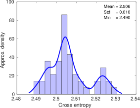
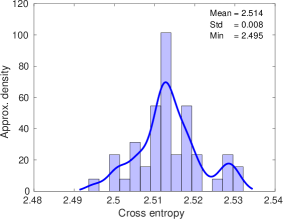
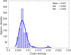
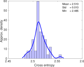
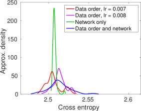
In the first experiment we study the empirical distribution of cross entropy values evaluated on the hold-out set by training 50 DNN networks for the BN50 task with different random seeds for the initial network parameters, while fixing the order of the mini batches. The results obtained with initial learning rates set to 0.007 and 0.008 are plotted in Figures 1(a,b) as both histograms and kernel density estimates using a Gaussian kernel (solid line). The difference in learning rate is not very large and the distributions are fairly similar except that the mean for the experiments with learning rate 0.007 is somewhat smaller than that of 0.008. In the next experiment we use a fixed random initialized of the network parameters, and then vary the random seed used for the batch randomization. With a learning rate of 0.008 this gives the distribution shown in Figure 1(c). As seen from the plot and as evident from the standard deviation, the distribution is tightly concentrated around its mean with the exception of one outlier. Next, we randomize both the initial parameters as well as the data order, while keeping the initial learning rate at 0.008. The results in Figure 1(d) show that the standard deviation grows and exceeds the sum of those in Figures 1(b) and (c). For reference we plot all kernel density estimates in Figure 1. From this plot it is clear just how localized the distribution of cross entropy values is when keeping the data order fixed and changing only the initial network parameters. This suggests that the data order is more important than the initial parameters in determining the final result. More experiments are needed to see if this applies only for this task, or whether it holds more generally.

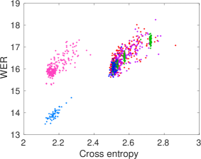
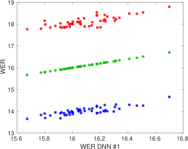
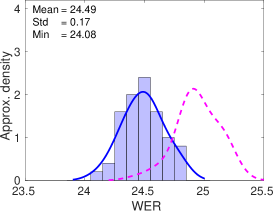
As mentioned in the introduction, the goal of ASR is to obtain a small word-error rate. In addition to the acoustic model, the word-error rate also depends on the decoder settings, the language model, and the relative weights of the language and acoustic models for computing likelihoods. In Figure 1(f) we plot the word-error rates for the above four settings against the cross-entropy. While the two are somewhat correlated, it does not hold that models with a lower cross entropy necessarily have a word-error rate as well. We also trained 50 instances of the BN400 DNN task with varying initial parameters and data orders. The results of these experiments appear in the bottom left corner of the figure. Finally, we trained 50 CNN instances on BN50, again with different initial parameters and data order. Even though the cross entropy is closer to the values obtained with the BN400 DNNs, the word-error rate only seems to improve marginally over the BN50 DNNs. It is not clear what causes this disparity, but it does clearly show the discrepancy between the training objective and the evaluation metric. To see how the performance of the models changes with different evaluation sets and language models, we plot in Figure 2 the results of three different decodes against the results from the BN50 DNN trained with learning rate 0.008, standard language model and evaluated on Dev04f. Overall the relative model accuracy roughly remain the same across evaluation sets and language models. In all three settings the best models remains the best and likewise for the worst model.

Figure 2: The word-error rates depend on the language model and evaluation set: (top) standard LM, evaluated on RT-04, (middle) standard LM, Dev-04f, and (bottom) large LM, Dev-04f. Results are plotted against the WER results in the middle.

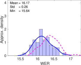
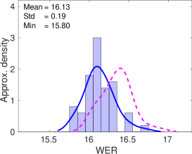
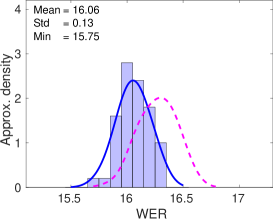
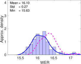
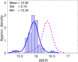
In Figures 3(a)–(d) we plot the empirical distribution of the WER for the four BN50 DNN experiments given in Figure 1(e). The blue histogram and kernel density estimation summarize the results obtained when using the optimal weight on the acoustic model relative to the language model. The dashed purple line shows the distribution that results when changing the acoustic weight to a sub-optimal value. The mean and standard deviation in WER values for the different setups reflect the relative values of the cross entropy values in Figures 1(a)–(d). The largest WER range of 15.6 to 17.1 is obtained when both the initial parameters and data order vary. Among the BN50 configurations tried, the results for the BN50 CNN setup in Figure 3(e) have the smallest mean and minimum WER. In addition, the standard deviation is small compared to the equivalent DNN in Figure 3(d).

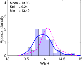
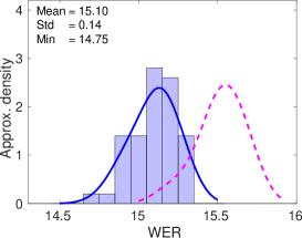
Increasing the amount of training data gives a large reduction in WER with the average going down from 16.1 to 13.98, as shown in Figure 3(e). The difference between the best and worst WER remains around 1.3 percent absolute, but the ratio between the standard deviation and the mean remains nearly the same being only slightly higher for the BN400 setup. Figures 3(g) and (h) give the distribution of WER for the 300-hour Switchboard system evaluated on the Hub5 and CallHome datasets. The standard deviation on these experiments is smaller than those for the different Broadcast News experiments.

(a) bn50-dnn, data order, lr = 0.007	(b) bn50-dnn, data order, lr = 0.008	(c) bn50-dnn, network only
(d) bn50-dnn, data order & network	(f) bn50-cnn, data order & network	(e) bn400-dnn, data order & network
(g) swb-dnn, Hub5	(h) swb-dnn, CallHome	(i) bn50-dnn, sequence training

Figure 3: Result obtained for different datasets and neural network types, as indicated next to the labels. Plots (a)–(d) show the results for BN50 DNN setups; (e) gives the results for the BN50 CNN system with varying data order and initial network parameters; (f) gives similar result for a BN400 DNN setup; (g,h) plot the results for the 300h switchboard DNN system when evaluated respectively on the Hub5 and CallHome datasets. The underlying acoustic for these two are the same and each of the 50 instances is trained with different random seeds for the data order and the initial network parameters. Finally, (i) gives the results obtained with sequence training.

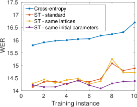
So far we have only considered experiments based on cross-entropy minimization using SGD. The best results in speech, see for example [10], are obtained using sequence-level discriminative training techniques. For our experiments we minimize the state-based minimum Bayes risk (MBR) objective [7, 13] using Hessian-free optimization [12]. As a starting point we took ten networks from the BN50 DNN setup in which both the data order and initial network parameters change and denote then by $n_{1}$ through $n_{10}$ in decreasing order of performance. For each of these networks we generated the corresponding enumerator and denominator lattices using a unigram language model, thus obtaining $\ell_{1}$ through $\ell_{10}$. We then applied sequence training to three settings: (1) Initial network $n_{k}$ and lattices $\ell_{k}$; (2) initial network $n_{k}$ and fixed lattice $\ell_{1}$; and (3) fixed initial network $n_{1}$ and lattices $\ell_{k}$. The resulting WERs are plotted in Figure 3(i) and connected by lines for clarity. All sequence-training results can be seen to improve substantially over the cross-entropy results. Interestingly, the starting point seems to be much more important than the network quality used to generate the lattices; initializing the network parameters with those of the best BN50 DNN cross-entropy system gives the best results among the three setups.

4 Discussion

When evaluating the performance of a new method there are two aspects that need to be taken into consideration. The first one concerns the statistical significance of results obtained for individual models. This includes techniques such as McNemar’s and matched-pair tests, as advocated in [14]. The second aspects goes beyond individual models and concerns the performance of methods as a whole. Currently, methods are evaluated by comparing with a baseline the very best model obtained after careful and often extensive fine tuning. The baseline may itself be a highly refined result reported in the literature, but equally often consist of a single run of a standard DNN or CNN system. Aside from the question of whether the two models are significantly different is the more important question of how meaningful it is to compare competing methods based on only one pair of models per dataset. As a though experiment, consider the situation where we compare the performance of the BN50 DNN from Figure 3(a) against itself. In particular, we consider the distribution in Figure 3(a) and compute the probability that, based on a matched-pair test with given confidence level, at least one of $n$ randomly sampled models is significantly better than a randomly sampled baseline. This gives:

Conf.	$n=1$	$n=2$	$n=5$	$n=10$	$n=20$
95.0%	35.0	54.7	81.9	95.1	99.5
99.0%	22.2	36.6	61.3	79.3	92.0
99.9%	11.3	19.7	36.4	51.7	66.8

It is seen that with sufficient sampling there is a high probability of finding a model that improves significantly over the baseline, and we would therefore conclude that the method improves upon itself! In practice a similar setting may arise when a high degree of fine tuning amounts not so much to finding the optimal parameters but rather to sampling repeatedly from similar distributions, thereby increasing the chance of eventually finding a good model instance. We see that even if a model obtained with a proposed method is significantly better than the baseline, it does not automatically allow us to conclude that the method as a whole is better than that used for the baseline.

When the training distribution of two methods were known (either based on an optimal set of hyperparameters, or on some distribution over these parameters) we could look at principled ways of comparing the performance. We could for example

1. Compare the best possible results; this provides a best-case scenario and provided that the baseline comes from a highly tuned system, this is what is commonly used. Note that this approach is biased in favor of the proposed method if the baseline is not extensively tuned (as illustrated above).

2. Compare the mean results; this says something about the performance of an average training run;

3. Determine the probability that a randomly sampled models of one method is better than that the other.

Of course, the entire distribution is not known and even obtaining a good approximation may require excessive sampling. For a comparison methodology to be practicable we require that it can be evaluated based on only a small number of samples, which is even more challenging if the underlying distribution is non-parametric. The performance of the first approach really depends on the probability mass contained in the lower tail; if this is small it will be very difficult to sample. When comparing the mean care needs to be taken; suppose that the means are identical. Then in terms of method performance it may be desirable to have a stable method with little variance. On the other hand, when it comes to obtaining a model for practical use, a larger variance will make it easier to sample the best model (here the goal really is to obtain the best possible model instance). For the third example criterion, we could sample pairs of models and apply a pairwise test and assign 1 for a win, $1/2$ for a draw, and 0 for losing. The sum of these values gives the relative performance of the methods, which can be quantified by testing against a binomial distribution with suitable $p$ values. Alternatively, a pairwise test over the results for each method combined can be done.

5 Conclusions

In the literature it is still common practice to report results without any information on the variance; see for example [15, 16, 17, 18]. There are of course some exceptions such as [19, 20], but even these papers only give variance on phone-error rate and not on WER. The improvements in the aforementioned papers may very well be meaningful and represent a significant improvement on the baseline method, but the problem is that based on individual numbers we simple cannot be sure. There is admittedly some additional difficulty in systems that rely on a large number of training stages. The sequence training setup discussed in the previous section is a simple example, but much more involved processing approaches in which each step is highly tuned exist [10]. Nevertheless, more insight into the result distributions for different settings and algorithms, and their incorporation into performance evaluation is much needed.

References

- [1] F. Seide, G. Li, and D. Yu, “Conversational speech transcription using context-dependent deep neural networks,” in Interspeech 2011. International Speech Communication Association, August 2011.
- [2] A. Choromanska, M. Henaff, M. Mathieu, G. B. Arous, and Y. LeCun, “The loss surfaces of multilayer networks,” arXiv:1412.0233, 2014.
- [3] R. Pascanu, Y. N. Dauphin, S. Ganguli, and Y. Bengio, “On the saddle point problem for non-convex optimization,” arXiv:1405.4604, 2014.
- [4] N. Pinto, D. Doukhan, J. J. DiCarlo, and D. D. Cox, “A high-throughput screening approach to discovering good forms of biologically inspired visual representation,” PLoS Comput Biol, vol. 5, no. 11, p. e100579, 2009.
- [5] G. Hinton, O. Vinyals, and J. Dean, “Distilling the knowledge in a neural network,” arXiv:1503.02531, 2015.
- [6] J. Fiscus, J. Garofolo, M. Przybocki, W. Fisher, and D. Pallett, “1997 English Broadcast News Speech (HUB4) LDC98S71,” 1998, linguistic Data Consortium.
- [7] B. Kingsbury, “Lattice-based optimization of sequence classification criteria for neural-network acoustic modeling,” in Proceedings of ICASSP, 2009, pp. 3761–3764.
- [8] J. Godfrey and E. Holliman, “Switchboard-1 Release 2 LDC97S62,” 1997, Linguistic Data Consortium, Philadelphia.
- [9] F.-H. Liu, M. Monkowski, M. Novak, M. Padmanabhan, M. Picheny, and P. S. Rao, “Performance of the IBM LVCSR system on the Switchboard corpus,” in Speech Research Symposium, 1995, p. 189.
- [10] G. Saon, H.-K. J. Kuo, S. Rennie, and M. Picheny, “The IBM 2015 English conversational telephone speech recognition system,” in Proceedings of Interspeech, 2015.
- [11] T. N. Sainath, B. Kingsbury, and B. Ramabhadran, “Improving training time of deep belief networks through hybrid pre-training and larger batch sizes,” in Proceedings of the NIPS Workshop on Log-linear Models, 2012.
- [12] J. Martens, “Deep learning via Hessian-free optimization,” in Proceedings of the 27th International Conference on Machine Learning (ICML), 2010.
- [13] B. Kingsbury, T. Sainath, and H. Soltau, “Scalable minimum Bayes risk training of deep neural network acoustic models using distributed Hessian-free optimization,” in Proceedings of Interspeech, 2012.
- [14] L. Gilick and S. J. Cox, “Some statistical issues in the comparison of speech recognition algorithms,” in Proceedings of the 1989 International Conference on Acoustics, Speech, and Signal Processing (ICASSP), vol. 1, May 1989, pp. 532–535.
- [15] T. N. Sainath, B. Kingsbury, A.-R. Mohamed, G. E. Dahl, G. Saon, H. Soltau, T. Beran, A. Y. Aravkin, and B. Ramabhadran, “Improvements to deep convolutional neural networks for LVCSR,” in 2013 IEEE Workshop on Automatic Speech Recognition and Understand (ASRU), December 2013, pp. 315–320.
- [16] T. N. Sainath, O. Vinyals, A. Senior, and H. Sak, “Convolution, long short-term memory, fully connected deep neural networks,” in Proceedings of ICASSP, 2015, pp. 4580–4584.
- [17] R. Zhao, J. Li, and Y. Gong, “Variable-component deep neural network for robust speech recognition,” in Proceedings of Interspeech, 2014.
- [18] J. Li, A. Mohamed, G. Zweig, and Y. Gong, “LSTM Time and frequency recurrence for automatic speech recognition,” in IEEE Automatic Speech Recognition and Understanding Workshop, December 2015. [Online]. Available: http://research.microsoft.com/apps/pubs/default.aspx?id=259285
- [19] A. Graves, N. Jaitly, and A.-R. Mohamed, “Hybrid speech recognition with deep bidirectional LSTM,” in 2013 IEEE Workshop on Automatic Speech Recognition and Understanding (ASRU), December 2013, pp. 273–278.
- [20] T. Moon, H. Choi, H. Lee, and I. Song, “RNNDrop: A novel dropout for RNNs in ASR,” in 2015 IEEE Workshop on Automatic Speech Recognition and Understand (ASRU), December 2015, pp. 65–70.