Max-Margin Feature Selection

Abstract

Many machine learning applications such as in vision, biology and social networking deal with data in high dimensions. Feature selection is typically employed to select a subset of features which improves generalization accuracy as well as reduces the computational cost of learning the model. One of the criteria used for feature selection is to jointly minimize the redundancy and maximize the relevance of the selected features. In this paper, we formulate the task of feature selection as a one class SVM problem in a space where features correspond to the data points and instances correspond to the dimensions. The goal is to look for a representative subset of the features (support vectors) which describes the boundary for the region where the set of the features (data points) exists. This leads to a joint optimization of relevance and redundancy in a principled max-margin framework. Additionally, our formulation enables us to leverage existing techniques for optimizing the SVM objective resulting in highly computationally efficient solutions for the task of feature selection. Specifically, we employ the dual coordinate descent algorithm (Hsieh et al., 2008), originally proposed for SVMs, for our formulation. We use a sparse representation to deal with data in very high dimensions. Experiments on seven publicly available benchmark datasets from a variety of domains show that our approach results in orders of magnitude faster solutions even while retaining the same level of accuracy compared to the state of the art feature selection techniques.

1 Introduction

Many machine learning problems in vision, biology, social networking and several other domains need to deal with very high dimensional data. Many of these attributes may not be relevant for the final prediction task and act as noise during the learning process. A number of feature selection methods have already been proposed in the literature to deal with this problem. These can be broadly categorized into filter based, wrapper based and embedded methods.

In filter based methods, features (or subset of the features) are ranked based on their statistical importance and are oblivious to the classifier being used (Guyon and Elisseeff, 2003; Peng et al., 2005). Wrapper based methods select subset of features heuristically and classification accuracy is used to estimate the goodness of the selected subset (Kumar et al., 2012). These methods typically result in good accuracy while incur high computational cost because of the need to train the classifier multiple number of times. In the embedded methods, feature selection criteria is directly incorporated in the objective function of the classifier (Tan et al., 2010; Yiteng et al., 2012). Many filter and wrapper based methods fail on very high dimensional datasets due to their high time and memory requirements, and also because of inapplicability on sparse datasets (Guyon and Elisseeff, 2003; Yiteng et al., 2012).

In the literature, various max-margin formulation had been developed for many applications (Burges, 1998; Guo et al., 2007). Recently, we have proposed a hard margin primal formulation for feature selection using quadratic program (QP) slover (Prasad et al., 2013). This approach jointly minimizes redundancy and maximizes relevance in a max-margin framework. We have formulated the task of feature selection as a one class SVM problem (Schölkopf et al., 2000) in the dual space where features correspond to the data points and instances correspond to the dimensions. The goal is to search for a representative subset of the features (support vectors) which describes the boundary for the region in which the set of the features (data points) lies. This is equivalent to searching for a hyperplane which maximally separates the data points from the origin (Schölkopf et al., 2000).

In this paper, we have extended the hard-margin formulation to develop a general soft-margin framework for feature selection. We have also modified the primal and dual formulations. We present the dual objective as unconstrained optimization problem. We employ the Dual Coordinate Descent (DCD) algorithm (Hsieh et al., 2008) for solving our formulation. The DCD algorithm simultaneously uses the information in the primal as well as in the dual to come up with a very fast solver for the SVM objective. In order to apply DCD approach, our formulation has been appropriately modified by including an additional term in the dual objective, which can be seen as a regularizer on the feature weights. The strength of this regularizer can be tuned to control the sparsity of the selected features weights. We adapt the liblinear implementation (Fan et al., 2008) for our proposed framework so that our approach is scalable to data in very high dimensions. We also show that the Quadratic Programming Feature Selection (QPFS) (Rodriguez-Lujan et al., 2010) falls out as a special case of our formulation in the dual space when using a hard margin.

Experiments on seven publicly available datasets from a vision, biology and Natural Language Processing (NLP) domains show that our approach results in orders of magnitude faster solutions compared to the state of the art techniques while retaining the same level of accuracy.

The rest of the paper is organized as follows. We describe our proposed max-margin formulation for feature selection (MMFS) including the dual coordinate descent approach in Section 2. We present our experimental evaluation in Section 4. We conclude our work in Section 5.

2 Proposed Max-Margin Framework

The key objective in feature selection is to select a subset of features which are highly relevant (that is high predictive accuracy) and non-redundant (that is uncorrelated). Relevance is captured either using an explicit metric (such as the correlation between a feature and the target variable) or implicitly using the classifier accuracy on the subset of features being selected. Redundancy is captured using metrics such as correlation coefficient or mutual information. Most of the existing feature selection methods rely on a pairwise notion of similarity to capture redundancy (Rodriguez-Lujan et al., 2010; Peng et al., 2005; Yu and Liu, 2003).

We try to answer the question ”Is there a principled approach to jointly capturing the relevance as well redundancy amongst the features?”. To do this, we flip around the problem and examine the space where features themselves become the first class objects. In particular, we analyze the space where ”features” represent the data points and ”instances” represent the dimensions. Which boundary could describe well the set of features lying in this space? Locating the desired boundary is similar to one class SVM formulation (Schölkopf et al., 2000). This equivalently can be formulated as the problem of searching for a hyperplane which maximally separates the features (data points) from the origin in the appropriate kernel space over the features. In order to incorporate feature relevance, we construct a set of parallel marginal hyperplanes, one hyperplane for each feature. The margin of each separating hyperplane captures the relevance of the corresponding feature. Greater the relevance, higher the margin required (a greater margin increases the chances of a feature being a support vector). Redundancy among the features is captured implicitly in our framework. The support vectors which lie on respective margin boundaries constitute the desired subset of features to be selected. This leads to a principled max-margin framework for feature selection. The proposed formulation for MMFS is presented hereafter.

2.1 Formulation

Let $X$ represent the data matrix where each row vector ${x_{i}}^{T}$ ($i\in 1\ldots M)$ denotes an instance and each column vector $f_{j}$ ($j\in 1\ldots N)$ denotes a feature vector. We will use $\phi$ to denote a feature map such that the dot product between the data points can be computed via a kernel $k(x_{i},x_{j})=\phi(x_{i})^{T}\phi(x_{j})$, which can be interpreted as the similarly of $x_{i}$ and $x_{j}$. We will use $Y$ to denote the vector of class labels $y_{i}$’s $(i\in 1\ldots M)$. Based on the above notations, we present the following formulation for feature selection in the primal:

$$\begin{array}[]{ll}\begin{aligned} {}&\min_{w,b}\quad\frac{1}{2}w^{T}w+b+C\sum_{i=1}^{N}\xi_{i}\\ \text{subject to}&~{}~{}~{}~{}w^{T}\phi(f_{i})+b\geq r_{i}-\xi_{i},~{}\xi_{i}\geq 0,~{}~{}\forall i=1,\ldots,N;\end{aligned}\end{array}$$ (1)

where, $w$ represents a vector normal to the separating hyperplane(s) , $b$ represents the bias term and $\xi_{i}$’s represent slack variables. $r_{i}$ captures the relevance for the $i^{th}$ feature. The equation of the separating hyperplane is given by $w^{T}\phi(f_{i})+b=0$ with the distance of the hyperplane from the origin being $-b$. Note that in this formulation the objective function is similar to the one class SVM (Schölkopf et al., 2000). However, the constraints are very much different as our formulation includes the relevance of the features ($r$). The choice of $\phi$ determines the kind of similarity (correlation) to be captured among the features. The set of support vectors obtained after optimizing this problem i.e. {$f_{i}\mid w^{T}\phi(f_{i})+b=r_{i}$} and the margin violators {$f_{i}\mid\xi_{i}>0$} constitute the set of features to be selected. In the dual space, this translates to those features being selected for which $0<\alpha_{i}\leq C$ where $\alpha_{i}$ is the Lagrange multiplier for $f_{i}$. We will refer to our approach as Max-Margin Feature Selection (MMFS). Note that when dealing with hard margin (no noise) case and the term involving $C$ disappears (since this enforces $\xi_{i}=0,\forall i$).

Figure 1 illustrates the intuition behind our proposed framework in the linear dot product space (with hard margin). In the figure, $w^{T}f+b=0$ represents the separating hyperplane. The distance of this hyperplane from the origin is given by $-b/||w||$. The first term in the objective of Equation 1 tries to minimize $w^{T}w$ i.e. maximize $1/||w||$. The second term in the objective tries to minimize $b$ i.e. maximize $-b$. Hence, the overall objective tries to push the plane away from the origin. The i^th dashed plane represents the margin boundary for the i^th feature. The distance of this marginal hyperplane from the separating hyperplane is given by $r_{i}/||w||$ where $r_{i}$ is the pre-computed relevance of the i^th feature. Therefore, minimizing $w^{T}w$ in the objective also amounts to maximizing this marginal distance ($r_{i}/||w||$). Hence, the objective has the dual goal of pushing the hyperplane away from the origin while maximizing the margin for each feature (weighted by its relevance)as well. The features which lie on the respective marginal planes are the support features (encircled points). The redundancy is explicitly captured in the dual formulation of this problem.

Fig. 1: Feature representation in sample space. The diagram is conceptual only.

2.2 Dual Formulation

In order to solve the MMFS optimization efficiently by Dual Coordinate Descent strategy, we require both the primal and dual formulations. The dual formulation for Equation 1 can be derived using the Lagrangian method. The Lagrangian function $L(w,b,\xi,\alpha,\beta)$ can be written as:

$$L(w,b,\xi,\alpha,\beta) =\min_{w,b}\quad\frac{1}{2}w^{T}w+b+C\sum_{i=1}^{N}\xi_{i}$$

$$+\sum_{i=1}^{N}\alpha_{i}(r_{i}-\xi_{i}-(w^{T}\phi(f_{i})+b))-\sum_{i=1}^{N}\beta_{i}\xi_{i}$$

Where, $\alpha_{i}$’s and $\beta_{i}$’s are the Lagrange multipliers. Now, the Lagrangian dual can be written as:

$$\max_{\alpha,\beta:\alpha_{i}\geq 0,\beta_{i}\geq 0}\quad\min_{w,b,\xi}\quad L(w,b,\xi,\alpha,\beta)$$ (2)

At the optimality, $\nabla_{w}L$, $\frac{\partial L}{\partial b}$ and $\frac{\partial L}{\partial\xi_{i}}$ (for all $i$) will be 0 i.e.

$$\nabla_{w}L=w-\sum_{i=1}^{N}\alpha_{i}\phi(f_{i})=0;\frac{\partial L}{\partial b}=1-\sum_{i=1}^{N}\alpha_{i}=0$$ (3)

$$\frac{\partial L}{\partial\xi_{i}}=C-\alpha_{i}-\beta_{i}=0$$

By substituting the values from Equation (3) into Equation (2) we get:

$$f\left(\alpha\right) =\max_{\alpha}\quad r^{T}\alpha-\frac{1}{2}\alpha^{T}Q\alpha$$ (4)

Subject to $$0\leq\alpha_{i}\leq C,i=1,...,M;~{}I^{T}\alpha=1.$$

This is similar to the standard SVM dual derivation (Schölkopf et al., 2000). The only difference is that while there is a single margin in standard SVM, the number of features here dictate the number of margins . We can equivalently rewrite the dual formulation of (4) as follows:

$$f\left(\alpha\right) =\min_{\alpha}\quad\frac{1}{2}\alpha^{T}Q\alpha-r^{T}\alpha$$ (5)

Subject to $$0\leq\alpha_{i}\leq C,i=1,...,M;~{}I^{T}\alpha=1.$$

Here, $Q$ is the similarity matrix whose entries are given by $Q_{ij}=k(f_{i},f_{j})$ where $k(f_{i},f_{j})=\phi(f_{i})^{T}\phi(f_{j})$ is the kernel function corresponding to the dot product in the transformed feature space. $r$ represents the vector of feature relevance. $\alpha$’s are the Lagrange multipliers. Note that the first term in the objective captures the redundancy between the features and the second term captures the relevance as in the case of QPFS formulation of (Rodriguez-Lujan et al., 2010). Hence, the connection between the redundancy and the relevance becomes explicit in the dual formulation. It should be noted that the dual objective bears a close similarity to the QPFS objective. We give the detailed comparison in Section 3. We can give relative importance to redundancy and relevance by incorporating a scaling parameter $\theta\in(0,1)$ in Equation (5) as follows:

$$f\left(\alpha\right) =\min_{\alpha}\quad\frac{1}{2}(1-\theta)\alpha^{T}Q\alpha-\theta r^{T}\alpha$$ (6)

Subject to $$0\leq\alpha_{i}\leq C,i=1,...,M;~{}I^{T}\alpha=1.$$

In the primal formulation (Equation (1)), this can be achieved by scaling the relevance scores by $\frac{\theta}{1-\theta}$, that is, replacing the constraints $w^{T}\phi(f_{i})+b\geq r_{i}-\xi_{i}$ by $w^{T}\phi(f_{i})+b\geq\frac{\theta}{1-\theta}(r_{i}-\xi_{i})$.

2.3 Choice of Metrics

The relevance of a feature in our framework is captured using the correlation between the feature vector and the class label vector. In our experiments, we have normalized the data as well as the target vector (class labels) so that it has zero mean and unit variance. Hence, the dot product between the feature vector and the target vector (normalized) estimates the correlation between them i.e. relevance of the $i^{th}$ feature can be computed as $r_{i}=|Y^{T}\phi(f_{i})|$. Some other appropriate metric which captures the predictive accuracy of a feature (such as mutual information(MI)) could also be used (Peng et al., 2005).

The redundancy is usually captured using correlation or mutual information in feature selection tasks (Peng et al., 2005). In our framework, the dot product space (kernel) captures the similarity (redundancy) among the features and the required similarity metric can be captured by selecting the appropriate kernel. The linear kernel ($f_{i}^{T}f_{j}$) represents the correlation among the features when the features are normalized to zero mean and unit variance . Since the value of the correlation ranges between $-1$ and $1$, a degree two homogeneous polynomial kernel defined over normalized data represents the squared correlation (i.e. ${\phi(f_{i})}^{T}{\phi(f_{j})}=(f_{i}^{T}f_{j})^{2}$). The choice of this kernel is quite intuitive for feature selection as it gives equal importance to the positive and negative correlations. A Gaussian kernel can also be used to approximate the mutual information (MI) (Gretton et al., 2005) which is the key metric for non-linear redundancy measure in feature selection problems (Peng et al., 2005; Rodriguez-Lujan et al., 2010). Since the MMFS formulation very closely matches the one class SVM formulation, any of the existing algorithms for SVM optimization either in primal or dual can be used. Next, we describe the use of Dual Coordinate Descent (DCD) algorithm (Hsieh et al., 2008) to obtain a highly computationally efficient solution for our feature selection formulation.

2.4 Dual Coordinate Descent for MMFS

Following equation (1), the number of variables and the number of constraints in the primal formulation are $M$+$1$ and $2N$, respectively, while from equation (6), it is seen that the corresponding numbers are $N$ and $2N$+$1$, respectively. Solving the primal (typically by using QP solvers) may be efficient ($O(M^{3})$) in the cases when $M\ll N$ (Shalev-Shwartz et al., 2007). Solving the dual using QP solvers requires $O(N^{2})$ space and $O(N^{3})$ time. Even solving the dual using sequential minimal optimization (SMO) based methods in practice has the complexity of $O(N^{2})$ (Fan et al., 2005). These high time and memory complexities limit the scalability of directly solving the primal or dual for data with a very large number of instances and features.

In many cases when the data already lies in a rich feature space, the performance of linear SVMs is observed to be similar to that of non-linear SVMs. In such scenarios, it may be much more efficient to train the linear SVMs directly. The dual coordinate descent methods have been well studied for solving linear SVMs using unconstrained form of the primal as well as dual formulations (Hsieh et al., 2008) who have shown that dual coordinate descent algorithm is significantly faster than many other existing algorithms for solving the SVM problem. Since our formulation very closely resembles the one class SVM formulation (with the exception of having a separate margin for each feature), we can easily adapt the Dual Coordinate Descent (DCD) algorithm for our case.

Following the unconstrained formulation for the SVM objective (Hsieh et al., 2008), the MMFS objective in the primal (using a linear kernel) can be written as:

$$\min_{w}\quad\frac{1}{2}w^{T}w+\frac{1}{\gamma}\frac{b^{2}}{2}+C\sum_{i=1}^{N}\xi(w;f_{i},r_{i})$$ (7)

where $\xi(w;f_{i},r_{i})$ denotes the loss function and $\gamma$ is a control parameter. Assuming standard $L1$ loss, $\xi(w,x_{i},r_{i})=\max(r_{i}-(w_{i}^{T}f_{i}+b),0)$. Note the slightly changed form of the objective compared to Equation (1) where the bias term $b$ has been replaced by a squared term $\frac{b^{2}}{2}$. The bias term can now be handled by introducing an additional dimension:

$$f^{\prime}_{i}\leftarrow[f_{i}\quad 1/\gamma]\qquad\qquad w^{\prime}_{i}\leftarrow[w_{i}\quad b]$$ (8)

Equation (7) can then be equivalently written as:

$$\min_{w^{\prime}}\quad\frac{1}{2}w^{\prime T}w^{\prime}+C\sum_{i=1}^{N}\xi(w^{\prime},f^{\prime}_{i},r_{i})$$ (9)

The dual of this slightly modified problem becomes:

$$f(\alpha) =\min_{\alpha}~{}\frac{1}{2}\left(\alpha^{T}Q^{\prime}\alpha+\gamma*(I^{T}\alpha)^{2}\right)-r^{\prime T}\alpha$$ (10)

subject to $$\quad 0\leq\alpha_{i}\leq C,\forall i;$$

where $Q^{\prime}$ is ($N$+$1$)$\times$($N$+$1$) matrix such that $Q^{\prime}_{ij}={f^{\prime}}_{i}^{T}f^{\prime}_{j}$. Comparing Equation (10) with Equation (6), we note that the constraint requiring $I^{T}\alpha=1$ is no longer needed because of the slightly changed form of the objective. In the unconstrained form of the dual, we are minimizing an additional term $(I^{T}\alpha)^{2}$ in the objective which is nothing but the square of the $L1$ regularizer over the feature weights. Note that this term in the objective effectively takes care of the original constraint $I^{T}\alpha=1$. The parameter $\gamma$ controls the strength of this regularizer and can be tuned to control the sparsity of the solution. The gradient of the objective w.r.t to $\alpha_{i}$ can be computed as follows:

$$G_{i}=(Q^{\prime}\alpha)_{i}+\gamma\sum_{i=1}^{N}\alpha_{i}-r^{\prime}_{i}$$

Using the fact $w^{\prime}=\sum_{j=1}^{N}\alpha_{j}f^{\prime}_{j}$ (set of Equations (3)), the gradient can be further reduced as:

$$G_{i}=f_{i}^{T}w^{\prime}+\gamma\sum_{i=1}^{N}\alpha_{i}-r^{\prime}_{i}$$

We adapt the Dual Coordinate Descent algorithm (Hsieh et al., 2008) for our MMFS problem. This algorithm works by optimizing the dual objective by computing the gradient based on the weight vector $w^{\prime}$ in the primal. This process is repeated with respect to each $\alpha_{i}$ in turn and the weight vector $w^{\prime}$ is updated accordingly. This translates into optimizing a one variable quadratic function at every step and can be done very efficiently. We name this approach MMFS-DCD in the paper, henceforth.

2.5 Complexity

Following (Hsieh et al., 2008), the MMFS-DCD approach obtains an $\epsilon$-accurate solution in $O(\log(1/\epsilon))$ number of iterations. Time complexity of a single iteration is $O(MN)$. Memory complexity of the DCD algorithm is $O(NM)$. For sparse datasets, the complexities depend on $\bar{N}$ instead of $N$, where $\bar{N}$ is the average number of non-zero feature values in an instance. The details about the proof of convergence are available in (Hsieh et al., 2008).

3 Relationship to Existing Filter Based Methods

Quadratic Programming Feature Selection (QPFS) (Rodriguez-Lujan et al., 2010) is a filter based feature selection method which models the feature selection problem as a quadratic program jointly minimizing redundancy and maximizing relevance. Redundancy is captured using some kind of similarity score (such as MI or correlation) amongst the features. Relevance is captured using the correlation between a feature and the target variable. One norm of the feature weight vector $\alpha$ is constrained to be $1$. Formally, the quadratic program can written as:

$$f\left(\alpha\right) =\min_{\alpha}\frac{1}{2}\left(1-\theta\right)\alpha^{T}Q\alpha-\theta r^{T}\alpha$$ (11)

Subject to $$\alpha_{i}\geq 0,i=1,...,N;~{}I^{T}\alpha=1.$$

$Q$ is an $N\times N$ matrix representing redundancy among the features, $r$ is an $N$-sized vector representing the feature relevance and $\alpha$ is an $N$-sized vector capturing feature weights. $\theta\in\left[0,1\right]$ is a scalar which controls the relative importance of redundancy (the $Q$ term) and the relevance (the $r$ term). QPFS objective closely resembles the minimal-redundancy-maximal-relevance (mRMR) (Peng et al., 2005) criterion. When $\theta=1$, only the relevance is considered (maximum Relevance) and when $\theta=0$ only redundancy among the features is captured. QPFS has also been shown to outperform many existing feature selection methods including mRMR and maxRel (Rodriguez-Lujan et al., 2010).

The form of the QPFS formulation above is exactly similar to our dual formulation (Equation 6) for an appropriate choice of kernel (similarity) function and $C=\infty$ (hard margin). Hence, the QPFS objective falls out as a special case of our max-margin framework in the dual problem space when dealing with hard margin. It should be noted that Lujan et al. (Rodriguez-Lujan et al., 2010) do not give any strong justification for the particular form of the objective used, other than the fact that it makes intuitive sense and seems to work well in practice. This is unlike our case where we present a max-margin based framework for jointly optimizing relevance and redundancy. Therefore, our formulation can be seen as providing a framework for the use of the QPFS objective and generalizing it further to handle noise (soft margin). Further, since no direct connection of the QPFS objective has been established with the SVM like formulation by Lujan et al. (Rodriguez-Lujan et al., 2010), the proposed approach for solving the objective is to simply use any of the standard quadratic programming implementations. Hence, the time complexity of QPFS approach is $O(N^{3}+MN^{2})$ and space complexity is $O(N^{2})$. To deal with cubic complexity, they propose combining it with the Nyström method which works on subsamples of the data. This can partially alleviate the problem with the computational inefficiency of QPFS but comes at the cost of significant loss in accuracy, as shown by our experiments. In our case, because of the close connection with the SVM based max-margin formulation and the ability to use the information from the primal as well as the dual, we can utilize any of the highly optimized SVM solvers (such as DCD which has time complexity linear in $N$).

Further it may be noted that while our MMFS-DCD approach can handle sparse representation of very high dimensional datasets, other feature selection methods like QPFS, FCBF, mRMR etc. cannot do so directly.

4 Experiments

4.1 Datasets

We demonstrate our experiments on seven publicly available benchmark datasets with medium to large number of dimensions. Out of these seven datasets Leukemia, RAOA and RAC are microarray datasets (Kumar et al., 2012), MNIST is a vision dataset (Tan et al., 2010) and REAL-SIM, Webspam and Kddb are the text classification datasets from NLP domain (Chang et al., 2010; Yiteng et al., 2012). Table 1 describes the details of the datasets. The last column represents the sparsity that is average number of non-zero features per instance in the dataset.

Table 1: Dataset description

Dataset	# Training	# Testing	# Features	Sparsity
Leukemia	72	-	7,129	7,129
RAOA	31	-	18,432	18,422
RAC	33	-	48,701	48,701
MNIST	11,982	1,984	752	752
REAL-SIM	57,848	14,461	20,958	51.5
Webspam	80,000	70,000	8,355,099	3,730
Kddb	100,000	748,401	29,889,813	30

4.2 Algorithms

We compared the performance of our proposed MMFS algorithm with FCBF (Yu and Liu, 2003), QPFS (Rodriguez-Lujan et al., 2010) and two other embedded feature selection methods, namely, Feature Generating Machine (FGM) (Tan et al., 2010) and Group Discovery Machine (GDM) (Yiteng et al., 2012). FGM uses cutting plane strategy for feature selection. GDM further tries to minimize the redundancy in FGM by incorporating the correlation among the features. QPFS, FGM and GDM have been shown to outperform a variety of existing feature selection methods including mRMR and MaxRel (Peng et al., 2005), FCBF (Yu and Liu, 2003), SVM-RFE (Guyon and Elisseeff, 2003), etc. For QPFS, we used mutual information (MI) as the similarity metric as it has been shown to give the best set of results (Rodriguez-Lujan et al., 2010). In MMFS-DCD, we use correlation of a feature vector with the target class vector to compute the feature relevance.

4.3 Methodology

We compare all the approaches for feature selection in terms of their accuracy and execution time on each of the datasets. For all the datasets except Webspam and Kddb, we report the accuracies obtained at varying number of top $K$ features ($K$ = $\{$2, 3, 4,…, 100$\}$) selected for each of the methods. For webspam and kddb datasets,we report the accuracies obtained at varying number of top $K$ features ($K$ =$\{$5, 10, 20, 30,…, 200$\}$) selected by FGM, GDM and MMFS-DCD methods.

We also report the best accuracies obtained at any given value of $K$ in the above range for all the datasets. We have normalized all the datasets except webspam and kddb to zero mean and unit variance. The zero mean and unit variance normalization for webspam and kddb datasets is very memory inefficient (very large memory ($>100GB$)) as these two are very large sparse datasets. We have normalized these two datasets with unit variance (Yiteng et al., 2012). In the microarray datasets, the number of samples are small so we report the leave-one-out cross-validation (LOOCV) accuracy. For MNIST and REAL-SIM datasets, training and testing splits are provided in (Chang et al., 2010). We have followed the training and testing splits of  (Yiteng et al., 2012) for webspam and kddb datasets. The results reported are averaged over $10$ random splits.

For MMFS-DCD, $\gamma$ parameter was tuned separately for each of the microarray datasets. The values of the parameters $C$ and $\theta$ were set to $1$ and $0.5$ respectively in all the experiments. We used the default settings of the parameters for both FGM and GDM as reported in (Tan et al., 2010; Yiteng et al., 2012). After the top $K$ features are selected, we used L2-regularized L2-loss SVM (Fan et al., 2008) with default settings (that is cost parameter $C$=1) for classification for each of the algorithms and for each of the datasets. MMFS was implemented on top of the liblinear tool. This implementation uses shrinking strategy (Hsieh et al., 2008). We used the publicly available implementation of QPFS (Rodriguez-Lujan et al., 2010). For FGM, we used the publicly available tool. GDM was implemented as an extension of the FGM based on the details given in Yiteng et. al (Yiteng et al., 2012). Any additional required wrapper code was written in C/C++. All the experiments were run on a Intel Core${}^{\text{TM}}$ i7 3.10GHz machine with 16GB RAM under linux operating system.

4.4 Results

4.4.1 Accuracy

Table 2 presents the best set of average accuracies (varying the number of top-K features selected) for all the methods. QPFS method did not produce any results on RAOA and RAC dataset within 24 hours. So, we used Nyström approximation (Rodriguez-Lujan et al., 2010) with sampling rate($\rho$=0.01) for these datasets. In the Figure 2(a), QPFS-N represents the QPFS with Nyström approximation. The QPFS and FCBF methods can not handle the sparse data, so we compare FGM, GDM and MMFS-DCD for webspam and kddb datasets. MMFS-DCD reaches the best accuracy on a small number of top $K$ features for all the microarray datasets. Further, MMFS-DCD produces significantly better accuracies compared to FCBF, QPFS, FGM and GDM on all the microarray datasets (FGM does equally well on RAC). On MNIST and webspam datasets, MMFS-DCD is marginally worse than the best performing algorithm. The plots for the average accuracies obtained as we vary the number of top $K$ features are available in the supplementary file. Clearly, for most of the datasets, MMFS-DCD is able to achieve the best set of accuracies at early stages of feature selection compared to all algorithms. Further, the gene ontology and biological significance of top selected genes for leukemia dataset is provided in the supplementary file.

4.4.2 Time

Figure 2 plots the average execution time for each of the methods. y-axis is plotted on a log scale. The time requirement for MMFS-DCD, FCBF and QPFS is independent of the number of features selected. For FGM and GDM, time requirement monotonically increases with $K$. For GDM, there is a sharp increase in the time required when $K$ becomes greater than five. It is obvious from Figure 2 that MMFS-DCD is upto several orders of magnitude faster than all the other algorithms on all the datasets.

Table 2: Best Accuracy (in %)

Dataset	FCBF		QPFS		FGM		GDM		MMFS-DCD
	Accuracy	M	Accuracy	M	Accuracy	M	Accuracy	M	Accuracy	M
Leukemia	90.28$\pm$0.1	37	87.50$\pm$ 0.1	45	87.5$\pm$0.1	2	84.72$\pm$0.1	2	91.67$\pm$0.1	6
RAOA	74.19$\pm$0.2	2	67.75$\pm$0.2∗	6	67.75$\pm$0.2	2	54.84$\pm$0.2	2	83.87$\pm$0.1	2
RAC	48.48$\pm$0.2	12	96.97$\pm$0.1∗	75	100.0$\pm$0.0	3	87.88$\pm$0.1	3	100.0$\pm$0.0	2
MNIST	91.07$\pm$0.0	19	96.06$\pm$0.0	94	96.21$\pm$0.0	99	96.67$\pm$0.0	77	96.06$\pm$0.0	83
REAL-SIM	-	-	-	-	90.03$\pm$0.01	90	89.48$\pm$0.01	100	90.19$\pm$0.01	100
Webspam	-	-	-	-	95.91$\pm$0.0	200	96.80 $\pm$ 0.0	200	96.79 $\pm$ 0.0	200
Kddb	-	-	-	-	87.60 $\pm$ 0.0	150	87.77 $\pm$ 0.0	190	88.39 $\pm$ 0.0	200

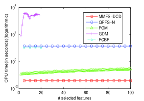
(a) RAC

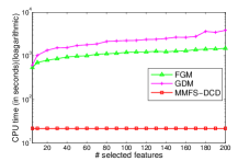
(b) webspam

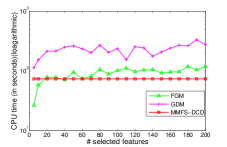
(c) kddb

Fig. 2: Comparison of execution time (in seconds) of MMFS-DCD with other methods for varying number of top $K$ features.

4.4.3 Parameter Sensitivity Analysis

Figure 3 presents the variation in accuracy for MMFS-DCD on the Leukemia dataset, as we vary the regularizer parameter ($\gamma$) with varying number of top $k$ features. The accuracy is not very sensitive to $\gamma$ as demonstrated by a large flat region in the graph.

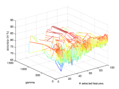
Fig. 3: Accuracy variation across $\gamma$ and top $k$ features

5 Conclusion and Future Work

We have presented a novel Max-Margin framework for Feature Selection (MMFS) similar to one class SVM formulation. Our framework provides a principled approach to jointly maximize relevance and minimize redundancy. It also enables us to use existing SVM based optimization techniques leading to highly efficient solutions for the task of feature selection. Our experiments show that MMFS with dual coordinate decent approach is many orders of magnitude faster than existing state of the art techniques while retaining the same level of accuracy.

One of the key future directions includes exploring if there is some notion of a generalization bound for the task of feature selection in our framework as in the case of SVMs for the task of classification. In other words, what can we say about the quality of the features selected as we see more and more data. We would also like to explore the performance of our model with non-linear kernels. Lastly, exploring the trade-off as we vary the noise penalty would also be a direction to pursue in the future.

References

- Burges (1998) Burges, C.J.C., 1998. A tutorial on support vector machines for pattern recognition. Data Min. Knowl. Discov. 2, 121–167.
- Chang et al. (2010) Chang, Y.W., Hsieh, C.J., Chang, K.W., Ringgaard, M., Lin, C.J., 2010. Training and testing low-degree polynomial data mappings via linear svm. J. Mach. Learn. Res. 11, 1471–1490.
- Fan et al. (2008) Fan, R.E., Chang, K.W., Hsieh, C.J., Wang, X.R., Lin, C.J., 2008. Liblinear: A library for large linear classification. J. Mach. Learn. Res. 9, 1871–1874.
- Fan et al. (2005) Fan, R.E., Chen, P.H., Lin, C.J., 2005. Working set selection using second order information for training support vector machines. J. Mach. Learn. Res. 6, 1889–1918.
- Gretton et al. (2005) Gretton, A., Herbrich, R., Smola, A., Bousquet, O., Schölkopf, B., 2005. Kernel methods for measuring independence. J. Mach. Learn. Res. 6, 2075–2129.
- Guo et al. (2007) Guo, Z., Zhang, Z., Xing, E.P., Faloutsos, C., 2007. A max margin framework on image annotation and multimodal image retrieval., in: ICME, IEEE. pp. 504–507.
- Guyon and Elisseeff (2003) Guyon, I., Elisseeff, A., 2003. An intoduction to variable and feature selection. Journal of Machine Learning Research 3, 1157–1182.
- Hsieh et al. (2008) Hsieh, C.J., Chang, K.W., Lin, C.J., Keerthi, S.S., Sundararajan, S., 2008. A dual coordinate descent method for large-scale linear SVM, in: Proceedings of the 25th International Conference on Machine Learning, ACM. pp. 408–415.
- Kumar et al. (2012) Kumar, P.G., Victoire, A.T.A., Renukadevi, P., Devaraj, D., 2012. Design of fuzzy expert system for microarray data classification using a novel genetic swarm algorithm. Expert Syst. Appl. 39, 1811–1821.
- Peng et al. (2005) Peng, H., Long, F., Ding, C., 2005. Feature selection based on mutual information: criteria of max-dependency, max-relevance, and min-redundancy. IEEE Trans. on Pattern Analysis and Machine Intelligence 27, 1226–1238.
- Prasad et al. (2013) Prasad, Y., Biswas, K., Singla, P., 2013. Feature selection using one class svm: A new perspective, in: MLCB, NIPS Workshop.
- Rodriguez-Lujan et al. (2010) Rodriguez-Lujan, I., Huerta, R., Elkan, C., Cruz, C.S., 2010. Quadratic programming feature selection. J. Mach. Learn. Res. 11, 1491–1516.
- Schölkopf et al. (2000) Schölkopf, B., Williamson, R.C., Smola, A.J., Shawe-Taylor, J., Platt, J., 2000. Support vector method for novelty detection. Advances in neural information processing systems 12, 582–588.
- Shalev-Shwartz et al. (2007) Shalev-Shwartz, S., Singer, Y., Srebro, N., 2007. Pegasos: Primal estimated sub-gradient solver for svm, in: Proceedings of the 24th International Conference on Machine Learning, ACM, USA. pp. 807–814.
- Tan et al. (2010) Tan, M., Wang, L., Tsang, I.W., 2010. Learning sparse SVM for feature selection on very high dimensional datasets, in: Proceedings of the 27th International Conference on Machine Learning, pp. 1047–1054.
- Yiteng et al. (2012) Yiteng, Z., Mingkui, T., Yew S., O., Ivor W., T., 2012. Discovering support and affiliated features from very high dimensions, in: Proceedings of the 29th International Conference on Machine Learning, pp. 1455–1462.
- Yu and Liu (2003) Yu, L., Liu, H., 2003. Feature selection for high-dimensional data: A fast correlation-based filter solution, in: Proceedings of the 20th International Conference on Machine Learning, pp. 856–863.