Kinetic effects observed in dynamic FORCs of magnetic wires. Experiment and theoretical description.

Abstract

This study is focused on the possibility to extend the use of the first-order reversal curve (FORC) diagram method to rate-dependent hysteresis. The FORCs for an amorphous magnetic wire was measured with an inductometric experimental setup in which the field-rate was maintained constant. The FORC experiment was performed for four different field-rates. As it is known, to obtain quantitative information on the magnetization process during the FORC process we need a model able to simulate as close as possible the experimental FORC diagrams. In this case, we have developed and implemented a model based on the hypothesis that the magnetization processes in this kind of materials are mainly due to the movement of a domain wall between the central domains of the wire. The differential equation of the domain wall movement is able to give a remarkably accurate description of the experimental FORC diagrams. The experimental FORCs, the FORC susceptibility diagram and the classical FORC diagram show however a number of details that the model is not able to describe. In each such case one discuss the possible physical cause of the observed behavior. As the magnetic wires are analyzed in many laboratories around the world for a wide variety of applications (essentially involving the control of the domain wall movement) we consider that our study offers to these researchers a valuable new tool.

I Introduction

One of the most successful new characterization technique, introduced in magnetism a few decades ago, known as the FORC diagram method, is gradually replacing the measurement of the major hysteresis loop that was predominant for a long time in the scientific literature. Originated in theoretical studies of ferromagnetic hysteresis based on the Classical Preisach Model (CPM) Preisach 1935 the idea of using first-order reversal curves (FORC) as a non-parametrical identification technique for this model was first published by Mayergoyz in 1985.Mayergoyz JAP 1985 As stated in this article, the most important point in using FORCs in the process of identification is that all the magnetic states of the systems are well defined in this type of experiment. However, originally the method was only recommended for the identification of the parameters of the CPM, that is, if and only if the hysteretic process has two properties: congruency of the minor loops measured within the same field limits and the wiping-out of the system memory after a closed minor loop (these systems are named CPM systems). Unfortunately most magnetic systems don’t obey to these two conditions and consequently it didn’t made too much sense to experimentalists to continue with the FORC measurement after they observed large disagreements from the congruency and/or wiping-out properties. This Gordian knot has been cut by a group Pike JAP 1999 from Davis University when they introduced a really efficient numerical tool to calculate a distribution from a set of FORCs covering the major hysteresis loop for a variety of samples and obtained in a systematic manner what they called FORC distributions for these samples. The fundamental new idea at that moment was that one can use the FORC distributions and the FORC diagrams, which are contour plots of these distributions, as tools of magnetic characterization for the samples. They have observed that the magnetic samples for a given category of magnetic material or system are similar but not identical and they introduced the idea of “fingerprinting” the material using FORC diagrams, idea which was really successful. As the authors claimed that the FORC method is not an identification technique for the Preisach model, the problem faced by the users of the method was how to interpret quantitatively these “fingerprints”, if at all possible. Systematic studies however have shown that it is counterproductive to deny the profound link between the FORC diagram method and the Preisach model Stancu JAP 2003 and that modified Preisach-type models like the moving Preisach model Della Torre 1965 could produce FORC diagrams very similar to a variety of experimental ones. This fact indicated that the FORC diagram method could become a quantitative method in some conditions. The main condition to transform the FORC method from a virtually qualitative one to a sound quantitative method is to find a model able to reproduce, using some fitting physical parameters, the experimental diagrams. Depending on the quality of this model, of its ability to describe not only one case but also systematic series of samples, the physical interpretation of the FORC diagrams becomes more and more trustworthy. As shown in Ref. Stancu JAP 2003, , many times the model can be a modified version of the Classical Preisach Model.

Nevertheless, many FORC diagram users are not employing properly this tandem experimental FORC/model but still are discussing their experimental results in quantitative terms. The most usual interpretation of the FORC distribution is as a vaguely distorted Preisach distribution. In this way, experimental FORC distributions are presented as estimates of the real distribution of the magnetic elements in the sample as a function of coercive and interaction fields. Of course, this is not exactly true and can be misleading in many cases. Many recent studies have shown what are the limits of this type of interpretation, especially if one expects to find physical elements related in a biunivocal way with a certain region on the FORC distribution.Dobrota JAP 2013 ; Dobrota PB 2015 ; Nica PB 2015 Similar discussions are specific not only to experimental magnetism and especially ferromagnetism, but also to the other areas of science in which FORC diagram technique is used to characterize complex hysteretic systems, like in ferroelectricity Stancu APL 2003 , temperature, light-induced and pressure hysteresis in spin-transition materials Tanasa PRB 2005 ; Enachescu PRB 2005 ; Rotaru PRB 2011 ; Kou AM 2011 , etc.

An important point that has to be discussed in details when quantitative interpretation of the FORC diagram is attempted is that in most experimental studies performed on magnetic samples showing hysteresis one assumes that the results are not essentially modified if the experimental time is changed within a certain margin. We also mention that most of the Preisach-type models are also time independent. Fundamentally, this means that the output value, which is the total magnetic moment of the studied sample, is not changing if the field is applied a shorter or longer duration. In fact, in experiments there are two distinct types of methods used for the measurement of the magnetic moment versus applied magnetic field curves. In one category of experiments the field is constant during the measurement of the magnetic moment, as in experiments with vibrating sample magnetometers (VSM). Another category, which is based on the electromagnetic induction phenomenon, implies a continuous variation of the applied magnetic field which produces a variation of the magnetic moment that is detected with appropriate systems of detection coils. If in the first experiment one can define a clear duration for the applied field in each experimental point, in the second one it is better to discuss the result as being influenced by the instantaneous value of the applied field and the field rate. Nevertheless, in both types of experiments in many concrete cases one can observe significant changes in the values of the measured magnetic moment as a function of experiment time (in the magnetometric measurements) or as a function of field rate (in the inductometric measurements). Both these phenomena could be included in the category of kinetic effects which may affect quite dramatically the results of measurements made on various magnetic samples. Of course these effects are related with the magnetic relaxation of the fundamental elements in the studied sample (particles, magnetic domains). It is also known for a long time that the distribution of the typical relaxation times within the sample is vital in the actual behavior of the magnetic sample as a function of the applied field and as a function of time.Street Wooley ; Neel

To investigate the kinetic effects on magnetic samples we have selected as samples magnetic wires. Isolated magnetic wires or systems of interacting wires are at this moment perhaps the most promising magnetic materials for a wide variety of applications. In a recently published monography Vazquez 2015 dedicated to the magnetic nano- and microwires one can find an illustration not only of the diversity of design and synthesis methods, but also of the wide range of applications for these materials. The first magnetic characterization of nanowire systems with the static FORC technique was published in 2004 Spinu IEEE 2004 and since then many groups have concentrated their attention on similar types of samples. Clime JAP 2007 ; Beron book 2010 ; Rotaru PRB 2011 ; Proenca Nanotechnology 2013 ; Almasi-Kashi PB 2014 In most of these articles the preferred measurement technique was the VSM and the dependence of the results on the waiting time in each experimental point was negligible. However, one of the most exciting applications of the magnetic wires is in microwave technology (see Chapter 17 in Ref. Vazquez 2015, ). The ac excitation field, especially as the frequency is increased, is fundamentally different from the quasistatic experiment. One certainly expects that the FORC diagrams to be strongly dependent on the frequency of the ac field and in this case we should unquestionably need a model to explain this behavior. In order to make a clear distinction between the quasistatic FORCs and the one in which the field rate is decisive in shaping the FORC distribution, we shall name the second one dynamic FORC (dFORC) diagram.

In this article we analyze the influence of the kinetic effects on dynamic FORC diagrams measured in an inductometric experimental setup, designed for magnetic wires. In the section dedicated to the experimental setup we present all the details concerning the control of the field rate during the FORC-type experiment. After we show the experimental results obtained for a sample measured for several values for the field rate, we have developed a simple model able to reproduce with a remarkable accuracy not only the typical features for one field rate but also how these features are changing when the field rate is changing. In this way one can provide with a high degree of certitude what are the connections between the experimental FORCs and physical phenomena related to the movement of the domain walls when an ac-type of magnetic field is applied to a magnetic wire.

II Experimental setup

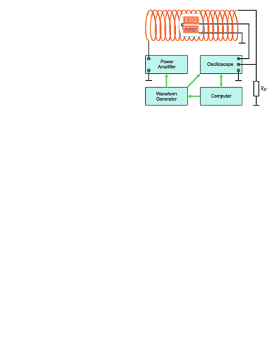
Figure 1: Block diagram of the induction magnetometer

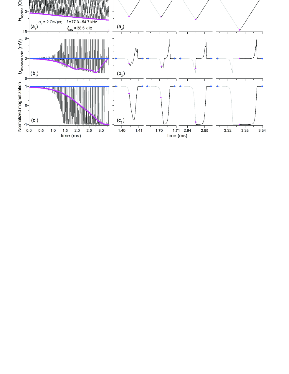
Figure 2: Time variation of the applied magnetic field [(a₁) and (a₂)] and of the induced signal across the detection coils [(b₁) and (b₂)] for a value of the field sweep rate of $\upsilon_{H}=2\,\mathrm{Oe/\mu s}$ used to obtain the dynamic FORCs and FORC diagram from Fig. 3(d₁). The last FORC is only used to obtain the dynamic major hysteresis loop (dMHL). The changing magnetic moment of the sample is proportional with the time integration of the induced signal. The triangle symbols mark the time moments when the applied field starts to increase on each FORC, i.e., when it is equal to the reversal field on each FORC, while the circles mark the time moments when the field attains its maximum value and then begins to decrease. Portions corresponding to decreasing fields are marked in gray. Moiré effect from (a₁-c₁) and is only an undesired visual artifact due to the proximity of the adjacent curves.

A FORC is obtained by saturating the sample under study in a positive magnetic field $H_{\mathrm{sat}}$, decreasing the field to the reversal field $H_{\mathrm{reversal}}$, and then sweeping the field back to $H_{\mathrm{sat}}$. The FORC is defined as the magnetization curve that results when the applied field is increased from $H_{\mathrm{reversal}}$ to $H_{\mathrm{sat}}$, and it is a function of the applied field $H_{\mathrm{applied}}$ and the reversal field $H_{\mathrm{reversal}}$. This process is repeated for many values of $H_{\mathrm{reversal}}$, so that the reversal points cover the descending branch of the major hysteresis loop (MHL), while the corresponding FORCs cover the hysteretic surface of the MHL. The FORC diagram is defined as the mixed second derivative of the set of FORCs with respect to $H_{\mathrm{applied}}$ and $H_{\mathrm{reversal}}$, taken with negative sign.Pike JAP 1999 Before each FORC measurement, saturation needs to be achieved in order to erase completely the previous magnetic history.

In order to measure the dynamic FORCs, an ac magnetometer based on the induction coil principle book induction magnetometer ; Beron RSI 11 was constructed. Two identical pickup/detection coils differentially connected (i.e., in series opposition so that the applied magnetic field produces no net signal/voltage) measure the sample’s magnetic response by detecting the induced voltage across the detection coils due to the changing magnetic moment of the sample which is placed within one of the coils (see Fig. 1). The detection coils should be as far apart to reduce both the mutual inductive coupling between them and the coupling between the empty detection coil and the magnetic sample. The coils geometry can be optimized for various sample shapes. Detection coils assembly is centered in a solenoid which provides the nearly uniform external excitation field [see Figs. 2(a₁) and (a₂) for the time variation of the applied field] through a function/arbitrary waveform generator (Picotest G5100A) and a high speed, broad band (dc to $1\,\mathrm{MHz}$) and high slew rate ($600\,\mathrm{V/\mu s}$ ) bipolar power amplifier (HSA 4011/HSA 4014 NF Corporation). The diameter of the solenoid should be few times bigger than that of the detection coils in order to have a uniform excitation field as well as to diminish the influence of the sample on the solenoid (i.e., the solenoid’s inductance should not depend on the magnetic sample). A high power and low inductance (over a wide frequency range) resistor $R_{H}$ connected in series with the solenoid allows to measure the electric current that flows through the solenoid and generates the external magnetic field (we note that the inductive reactance of the usual high power resistors can not be neglected beside its resistance even for low frequencies). The capability of supplying high output voltage and high power of the amplifier allow us to obtain up to $800\,\mathrm{Oe}$. For reliable measurements made on soft magnetic materials, a Helmholtz coil assembly could be used to compensate the Earth’s magnetic field. Time variation of the applied field (which is proportional to the voltage across the low inductance resistor $R_{H}$) and of the induced signal in the detection coils were digitized and acquired through a high resolution DPO7254 Tektronix digital oscilloscope ($2.5\,\mathrm{GHz}$ bandwidth and $10\,\mathrm{GS}\left/\mathrm{s}\right.$ synchronous real time sampling rate on all four input channels) synchronized with the waveform generator, and then sent to a computer for software signal processing. The high input impedance of the oscilloscope determines a very low (practically zero) current in the detection coils. Average acquisition mode was used to obtain the average value for each record point over many acquisitions, in order to reduce random noise. To further reduce the noise we have used the advantage of digital filtering which improves signal-to-noise performance over analog filters, which have to sacrifice accuracy in order to perform over a wide frequency band. No external amplifier was used for the induced voltage, only the internal amplifier of the oscilloscope. The high speed acquisition allows fast and detailed dynamic FORC diagrams measurement in a wide range of the applied field sweep rate values. All the instrumentation are interconnected with a computer via GPIB interface and assisted by a computer program generating also the waveforms needed.

In order to obtain a set/sequence of FORCs, a series of triangular voltage pulses with increasing amplitude [see Figs. 2(a₁) and (a₂)] is generated and applied to the solenoid via the high speed amplifier. The frequency of an ideal triangular wave for each FORC can be defined as $f=\upsilon_{H}\left/2\left(H_{\mathrm{sat}}-H_{\mathrm{reversal}}\right)\right.$, where $H_{\mathrm{sat}}$ and $H_{\mathrm{reversal}}$ are the saturation and reversal field, respectively, while $\upsilon_{H}$ is the applied field sweep rate. The saturation field was chosen so that the hysteresis properties of the magnetic sample no longer change when larger field amplitudes are applied. Frequency $f$ decreases as $H_{\mathrm{reversal}}$ decreases from $+H_{\mathrm{sat}}$ to $-H_{\mathrm{sat}}$. Using a triangular signal we obtain a linear variation of the applied field as a function of time (i.e., a constant $\upsilon_{H}$ on each FORC), what is useful in the analysis of the kinetic effects, which are also time dependent. Of course, a FORC sequence with a constant frequency $f$ can be used, but this complicates the results’ analysis because in this case the sweep rate will increase as the reversal field decreases. In addition, maintaining a constant frequency and increasing/decreasing the signal’s amplitude, sweep rate will increase/decrease as well. Moreover, using a sinusoidal signal would give rise to strong nonlinear phenomena.

The frequency spectrum of a triangular wave contains only odd harmonics which amplitude decreases proportional to the inverse square of the harmonic number. Critical to the production of the fast transitions in the applied magnetic field $H_{\mathrm{applied}}$ is the high speed, broad band linear amplifier, able to amplify as many harmonics of $f$. Leaving out the high frequency components has an effect of smoothing the $H_{\mathrm{applied}}$ versus time curve. The frequency response is limited also by the ratio of the inductance/reactance to the resistance of solenoid and $R_{H}$ assembly, ratio that should be as small as possible (e.g., using the lowest possible number of turns in the solenoid construction or decreasing their diameter, while the maximum value of $R_{H}$ is limited by the amplifier’s maximum output voltage). The inductance should be as small as not to block the high frequencies. Additionally, there is always non-zero capacitance between any two conductors which can be significant at high frequencies with closely spaced conductors. At low frequencies parasitic capacitance can usually be ignored, but in high frequency circuits it can be a problem because the parasitic capacitance will resonate with the inductance at some high frequency making a self-resonant inductor, leading to parasitic oscillations. Above this self-resonant frequency the inductor actually has capacitive reactance, as well. Consequently, in designing a dynamic FORC magnetometer is important to use coils (both the solenoid that creates the excitation field and the detection coils) with a self-resonant frequency higher than the frequency of the applied signal. The stray inductance and capacitance can be minimized for example by careful separation of turns, wires and components and by keeping the leads very short. Frequency dependent impedances are sources of systematic errors that should be considered in the analysis of experimental dynamic FORCs. The frequency dependence of the impedance of our coils was measured using a precision LCR meter and we have found the self-resonant frequency higher than $2\,\mathrm{MHz}$. Due to increased inductive reactance with increasing frequency as $\upsilon_{H}$ increases (i.e., the high frequency content of $H_{\mathrm{applied}}$ increases) a rounding of the tips of the triangular signals is obtained, and consequently the instantaneous field sweep rate around the reversal field is variable and smaller. Accordingly, when the decreasing applied field approaches the reversal field $H_{\mathrm{reversal}}$ the paths taken by the magnetic moment differ from the major hysteresis loop - see Figs. 3(a₁-d₁) where in the dFORCs the gray curves represent the portions with a decreasing field. This is another source of systematic errors in obtaining high sweep rate dynamic FORCs, but only affecting the results around $H_{\mathrm{applied}}=H_{\mathrm{reversal}}$. Throughout this paper we have calculated the experimental sweep rate on each FORC as the slope of a linear fit both on the decreasing as well as increasing part of the applied field, after removal of the first and last quarter of each part in order to eliminate the effect of rounded tips. As a result of solenoid’s inductance, the current through it lags behind the applied voltage, and accordingly behind the waveform generator’s synchronization signal, by a phase angle depending on inductance and $\upsilon_{H}$, and therefore the acquired signals by the oscilloscope start with a portion that actually belong to the last FORC. This should be considered in the subsequent numerical processing of data.

Another problem related to signal generation for the excitation field is related to how the waveform generator produces a piece-wise linear function (as the signal that we need) from a finite number of discrete points who are sent by the user from the remote interface to generator. The staircase approximation which is used by our generator leads to unwanted oscillations induced in the detection coils, and this effect is more important at low frequencies. The width of the steps in the staircase approximation can be reduced by increasing the number of points sent from the remote interface, the maximum number of points that can be sent being a characteristic of each generator (in our case $262,114$). This maximum number limits the number of FORCs that can be generated in a measurement, i.e., limits the value of $\Delta H_{\mathrm{reversal}}$ increment from FORC diagrams. Initially we have generated a waveform so that $H_{\mathrm{reversal}}$ starts from $+H_{\mathrm{sat}}$ and decreases up to $-H_{\mathrm{sat}}$, so that the entire hysteresis loop is covered, then we have made a “zoom” generating only the FORCs that are distinct from one another and distinct from the ascending branch of the hysteresis loop (see Fig. 2). In this way the $\Delta H_{\mathrm{reversal}}$ increment decreases and FORC diagrams with a better resolution are obtained.

From Figs. 2(b₁) and (b₂) we observe that the induced signal in the detection coils exhibits rapid variations with sharp peaks which imply high frequencies, and to capture these features we need short sampling in the acquisition process. High sampling frequency is essential when investigating dynamic magnetic properties, because low sample rate distorts the original signal, while high sample rate can properly reproduce the real signal. For a fast measurement of FORC diagrams, with a good resolution, we have used the high speed acquisition systems of a DPO7254 Tektronix digital oscilloscope. If a data acquisition card with a lower sample rate is available, then the signal presented in Fig. 2(a₁) should be broken up into smaller pieces, with smaller numbers of FORCs, measure the corresponding FORCs, and finally the pieces are added back together. Generation of each piece should be done so as to maintain the same field sweep rate.

The raw experimental data were first smoothed using a numerical FFT (fast Fourier transform) filter, the induced signal was numerically integrated to obtain the dynamic FORCs, and each FORC was numerically corrected for drift using the saturation values. In order to reduce the errors due to the miss-compensation of the detection coils, the signal induced in the detection coils with no sample in was acquired, and afterwards it was subtracted from the signal with sample. Because the mixed derivative from the FORC diagram’s definition significantly amplifies the measurement noise, the sensitivity of the measurement technique is important, as is the smoothing and numerical differentiation method applied to the raw data.

III Results

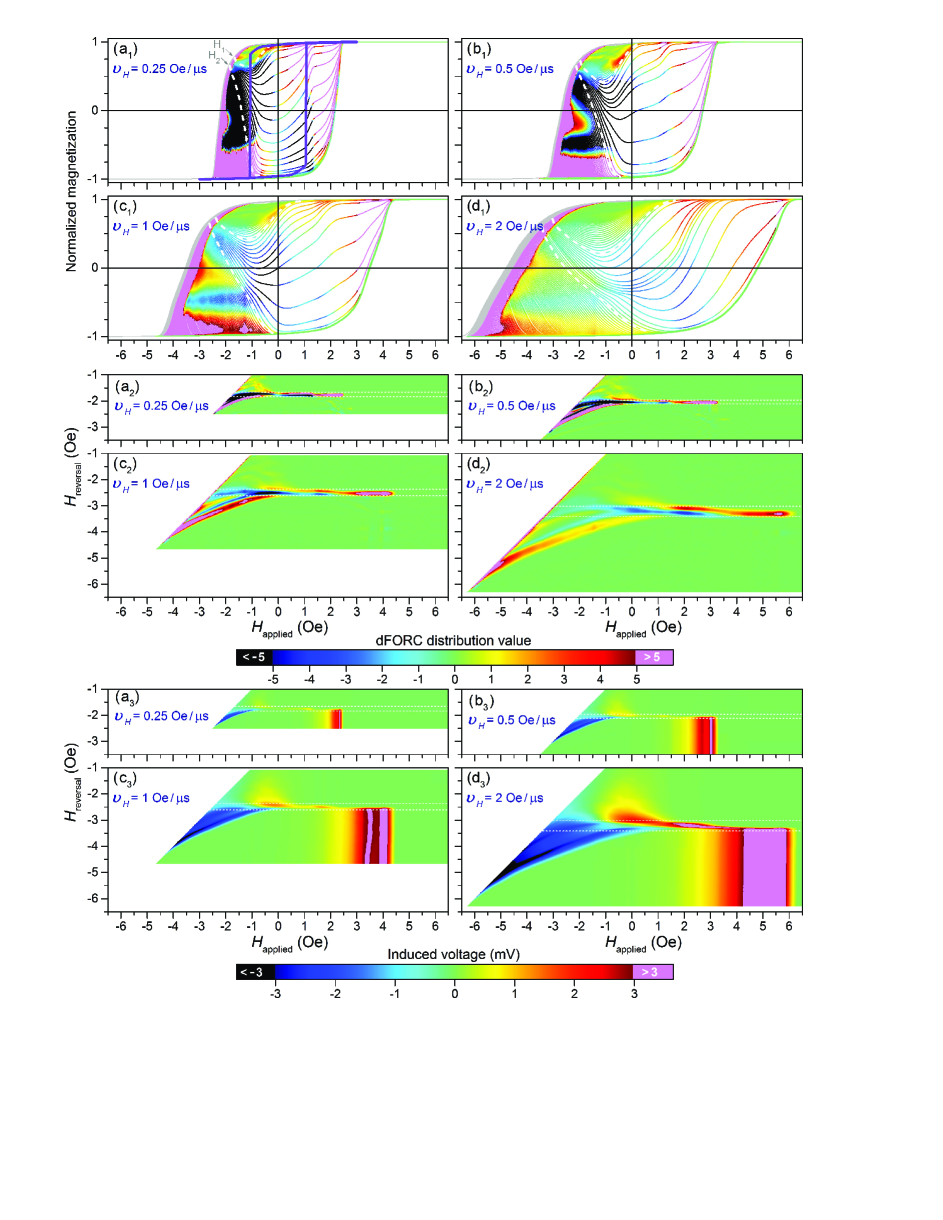
Figure 3: Experimental normalized dFORCs (a₁-d₁), dFORC diagrams (a₂-d₂), and induced voltage (which is proportional with the differential susceptibility $\chi_{\mathrm{differerntial}}$) in the detection coils (a₃-d₃) for different values of the applied field sweep rate $\upsilon_{H}$. The thick curve from (a₁) represents the quasistatic MHL measured with a VSM. The gray curves from dFORCs represent the portions corresponding to a decreasing field. Due to the dynamic effects the magnetic moment continues to decrease even after $H_{\mathrm{applied}}$ starts to increase. The dotted white curves delimit three regions: (i) $H_{1}<H_{\mathrm{reversal}}<+H_{\mathrm{sat}}$: the corresponding dFORCs either coincide with the descending branch of dMHL, or rapidly converge towards it, these dFORCs mainly covering the upper-left corner of dMHLs’ interior; (ii) $H_{2}<H_{\mathrm{reversal}}<H_{1}$: the corresponding dFORCs cover the most of dMHLs’ interior; and (iii) $-H_{\mathrm{sat}}<H_{\mathrm{reversal}}<H_{2}$: the corresponding dFORCs converge towards the ascending branch of dMHL, these dFORCs mainly covering the lower-left corner of dMHLs’ interior.

Figure 4: Coercive field measured on dMHLs as a function of sweep rate. The star marks the coercive field measured on the quasistatic MHL.

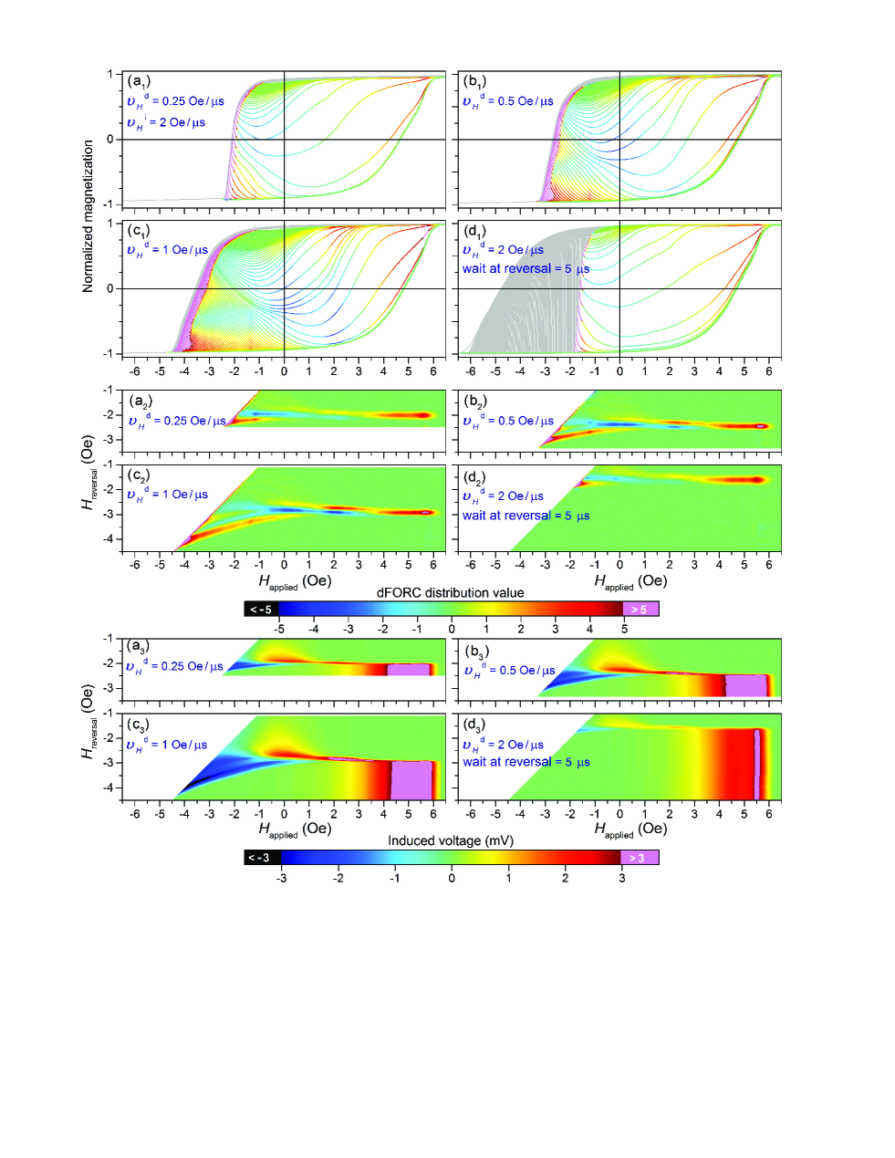
Figure 5: Similar with Fig. 3, but for different values of the decreasing applied field sweep rate (a-c) and for a waiting time of $5\,\mathrm{\mu s}$ at the reversal points (d), while the increasing applied field sweep rate has the same value $\upsilon_{H}^{i}=2\,\mathrm{Oe}\left/\mathrm{s}\right.$ for all cases [value corresponding to Figs. 3(d)].

All the experiments were performed at room temperature, on a $\mathrm{Fe}_{75}\mathrm{B}_{15}\mathrm{Si}_{10}$ $7\,\mathrm{mm}$ long amorphous glass-coated microwire with the diameter of the metallic nucleus of $8.5\,\mathrm{\mu m}$ and the glass coating thickness of $6.5\,\mathrm{\mu m}$. The magnetic domain structure of these wires typically consists of an inner core axially magnetized, occupying most of the microwire’s volume, surrounded by an outer shell (OS) containing domains with radial easy axes of magnetization (see, e.g., Ref. Vazquez 2015, ). Such materials are a cheaper alternative to nanowires prepared using various lithographic techniques, while their magnetic properties can be tailored in a wide range through composition or sample dimensions.Vazquez 2015 ; Zhukov 2009 The external magnetic field was applied parallel to the wire axis. During our experiments that measured the dynamic MHLs and FORCs the sample was entirely placed in one of the detection coils, so that the induced signal is due to the time variation of the microwire’s total magnetic moment. Throughout this paper the magnetization curves are normalized to saturation.

The quasistatic major hysteresis loop (MHL) measured with a vibrating sample magnetometer (VSM), and represented with a thick curve in Fig. 3 (a₁), indicates that the uniaxial magnetic anisotropy of the magnetic wire determines virtually a bistable magnetic behavior between two stable axially magnetized states. However, the loop is not perfectly rectangular, but is slightly rounded near the switching/coercive field. As the applied field is reduced from its maximum value, there is a first region in which the normalized magnetization $m$ decreases slowly from $1$ to about $0.94$. This region can be mainly attributed to the magnetization rotation in the outer shell, from the axial direction to perpendicular directions, at remanence the total magnetization of the outer shell being equal to zero. The magnetization of the entire wire at remanence is $0.95$. Concurrently begins the formation of closure domain structures at the ends of the wire, where the spins re-distribute to reduce the magnetostatic/stray energy. Further decrease of the applied field results in a much quicker decrease of the magnetization to about $0.8$, and it can be linked to an angular magnetization reorientation and/or by an enlargement of the closure structures. The third region of the quasistatic MHL is the one step reversal of the magnetization, also known as the large Barkhausen effect.

The rectangular-shaped hysteresis loop indicates that after the formation of the closure domains, the magnetization reversal process between the two stable magnetic configurations occurs by depinning and propagation of a domain wall (DW) inside the single domain inner core, from the closure structure at one end of the wire (see, e.g., Refs. Zhukov 2009, ; Ipatov JAP 2009, ; Varga PRL 2005, ; Vasquez PRL 2012, ; Ye JAP 2013, ; Zhukova JAC 2014, ). The switching is determined by the field needed to nucleate the reverse domain. With increasing wire length, increases the probability of nucleating some new additional reversed domains and new domain walls inside the wire (see, e.g., Refs. Ipatov JAP 2009, ; Corodeanu RSI 2011, ; Ovari 2012, ). The control of the magnetization reversal process and particularly of the domain wall’s motion is essential for the development of novel applications using magnetic wires. Due to the sudden decrease in magnetization at the switching point, the interior part of the quasistatic MHL can not be covered by quasistatic FORCs.

Since the microwires show in many cases inhomogeneities in their properties (geometry imperfections/defects, surface roughness produced during the fabrication process, impurities, or compositional irregularities ascribed to the amorphous structure), several pieces of wires were measured, all pieces having the same length, but being cut from different portions of an initial long wire. The quasistatic MHLs are similar, rectangular-shaped, only small variations of the switching field from sample to sample. However, even if the dynamic major hysteressis loops are also similar, the dynamic FORCs have features that are distinctive for each sample. The dFORCs have main characteristics which are common for all the investigated samples, but they also have fine distinguishing features that differ from sample to sample. The dFORCs have proven to be a much more sensitive tool in regard with the hysteresis loop, revealing various distinctive features of the magnetization switching, revealing the contribution of local inhomogeneities on the peculiarities of DW propagation, and therefore a useful tool for investigating the fine details of the magnetization dynamics and reversal. This method can be used also as a fast, nondestructive method for investigating the samples’ homogeneity.

In Fig. 3 are presented the experimental normalized dynamic FORCs (a₁-d₁) for one of the samples, the corresponding dynamic FORC diagrams (a₂-d₂), and the induced voltage measured across the detection coils (a₃-d₃), for different values of the applied field sweep rate $\upsilon_{H}$, the sweep rate of the decreasing field being equal to that of the increasing field. The gray curves from dFORCs represent the portions corresponding to a decreasing field. One observes that both the dMHL and dFORCs as well dFORC diagrams are dependent on the sweep rate.

We observe that an increase in sweep rate $\upsilon_{H}$ increases the slope of the vertical regions of the dynamic hysteresis loops, with respect to the quasistatic hysteresis. This phenomenon can be attributed to the counterbalance between the time required for the $+H_{\mathrm{sat}}$ to $-H_{\mathrm{sat}}$ variation, and the switching time related to the time needed for DW propagation along the whole wire. This kind of hysteresis is often referred to as rate-dependent hysteresis. The coercive field (defined as the field at which the projection of the magnetization on the applied field direction is zero) increases as $\upsilon_{H}$ increases (see also Fig. 4).

In Figs. 3 one observes that due to the dynamic effects the magnetic moment continues to decrease even after the applied magnetic field starts to increase. The last FORC (with the smallest $H_{\mathrm{reversal}}<0$ value) gives in fact the dynamic major hysteresis loop (dMHL). We note that the frequency $f_{\mathrm{MHL}}$ is provided in Fig. 2 only as guidance, the sweep rate $\upsilon_{H}$ being in fact the parameter which properly describes dMHLs, dFORCs, and dFORC diagrams, because the kinetic effects depend on $\upsilon_{H}$. Due to the rounding of the tips of the triangular applied field, the magnetization curves differ from the dynamic hysteresis loop when the decreasing applied field approaches the reversal field [see the gray portions in dFORCs in Figs. 3(a₁-d₁)]. Owing to the dynamic/kinetic effects the magnetization continues to decrease even after the applied magnetic field starts to increase, after the reversal points, i.e., there is a lag of the output (magnetization) with respect to the input (excitation applied magnetic field). These portions correspond to a negative induced voltage across the detection coils. The lag between magnetization and the applied field is more prominent as $\upsilon_{H}$ increases. Usually a lag between input and output is associated with a complex variable, i.e., with a real and imaginary component, the imaginary component indicating the dissipative processes in the sample. Hereby we can define the dynamic complex FORC (dcFORC).

We can define three regions in the dFORCs from Figs. 3 (a₁-d₁): (i) $H_{1}<H_{\mathrm{reversal}}<+H_{\mathrm{sat}}$ for which the corresponding dFORCs either coincide with the descending branch of dMHL, or rapidly converge towards it, these dFORCs mainly covering the upper-left corner of dMHLs’ interior; (ii) $H_{2}<H_{\mathrm{reversal}}<H_{1}$ for which the corresponding dFORCs cover the most of dMHLs’ interior; and (iii) $-H_{\mathrm{sat}}<H_{\mathrm{reversal}}<H_{2}$ for which the corresponding dFORCs converge towards the ascending branch of dMHL, these dFORCs mainly covering the lower-left corner of dMHLs’ interior. The borders between these regions are marked with dotted white curves in Fig. 3.

The dFORCs from the first region can be associated with almost reversible magnetization processes related to the generation of the closure domain structure. As the field $H$ is not sufficient to generate large scale propagation of the walls on these FORCs, what one observes are the processes of wall nucleation when the field is negative and with increased absolute value and as soon as the field is again increasing on each FORC the wall disappears as the positive saturation is attained. When the negative field is sufficient to start a considerable propagation of the wall towards the negative saturation the FORCs are significantly different. This is the second region on the set of FORCs and the richest in information due to the fact that these FORCs are actually covering a major part of the dMHLs’ interior.

One observes that these dFORCs have several inflection points which demarcate portions with different slopes on a given dFORC, the slope giving the differential susceptibility $\chi_{\mathrm{differerntial}}$. The inflection points that are near the ascending branch of the quasistatic hysteresis loop in Fig. 3(a₁) separate portions with very different slopes, which leads to the idea of switching of two different magnetic “entities,” such as the inner core and the outer shell of the microwire, the coercive field or the end of the switching of the outer shell being given by the inflection points. We note that these switching events are not very visible on dMHL. The magnetic field corresponding to the inflection points increases with increasing sweep rate. The portions of dFORCs located to the left of these points give rise to a pair of negative and positive peaks on the diagram, while the portions located to the right give rise to a single positive peak. The peaks with $H_{\mathrm{applied}}>0$ in the dFORC diagrams are mainly given by the dFORCs from the second region, but because the $\left[H_{1},H_{2}\right]$ interval is rather narrow, the FORC diagram features are constraint along a horizontal line, parallel with the $H_{\mathrm{applied}}$ axis, in contrast with most of the results presented in the scientific literature (where usually the FORC diagram’s peaks lie along the $H_{\mathrm{applied}}=H_{\mathrm{reversal}}$ and/or $H_{\mathrm{applied}}=-H_{\mathrm{reversal}}$ diagonals). While both fields $H_{1}$ and $H_{2}$ indicating the second region on the FORC set are gradually shifting towards more negative fields with increasing sweep rate, the width of the $\left[H_{1},H_{2}\right]$ interval increases in the same time.

For the dFORCs from the third region, the magnetization’s reversal started on the descending branch of dMHL can not be stopped by the increasing applied field, the magnetic wire reaching the negative saturated state, and then going back to the positive saturated state. The ascending part of these dFORCs coincide with the ascending branch of dMHLs (the induced voltage in the detection coils being the same), giving no peaks in the corresponding regions of the dFORC diagrams. The descending part of these dFORCs gives rise to several positive and negative peaks in diagrams, peaks that start along the $H_{\mathrm{applied}}=-H_{\mathrm{reversal}}$ diagonal (which in the Preisach model corresponds to the coercive field axis) and converge towards the “horizontal” peaks generated by the dFORCs from the second region. These peaks displaces down on the $H_{\mathrm{reversal}}$ axis with increasing sweep rate. All peaks broaden as $\upsilon_{H}$ increases.

In Figs. 3(a₃-d₃) the induced voltage in the detection coils is presented in the FORC coordinates, i.e., as a function of $H_{\mathrm{applied}}$ and $H_{\mathrm{reversal}}$. The induced voltage is proportional with the rate of change of the sample’s magnetization, i.e., with the derivative $dm\left/dt\right.$ of the magnetization with respect to time. Taking into account that $dm\left/dt\right.=\left(dm\left/dH_{\mathrm{applied}}\right.\right)\left(dH_{\mathrm{applied}}\left/dt\right.\right)=\upsilon_{H}\left(dm\left/dH_{\mathrm{applied}}\right.\right)=\upsilon_{H}\,\chi_{\mathrm{differerntial}}$, the induced voltage would be proportional with the derivative of the magnetization with respect to applied field, i.e, with the differential susceptibility $\chi_{\mathrm{differerntial}}$, for a perfect triangular applied field. However, as we have shown in the experimental setup description, due to the rounding of the tips of the triangular signals from Fig. 2(a₁), the instantaneous field sweep rate around the reversal field is variable. Nevertheless, excepting the region close to $H_{\mathrm{applied}}=H_{\mathrm{reversal}}$, for a given sweep rate $\upsilon_{H}$, the induced voltage from Figs. 3(a₃-d₃) is proportional with the differential susceptibility.

The results we have discussed already are rising the problem that even if the FORCs are measured only when the field is increasing, the results might be dependent also on the magnetization processes during the preparatory steps performed in experiment to generate the initial points on each FORC, when the field is actually decreasing. We have designed a few experiments to evidence this dependency.

In Figs. 5(a-c) the sweep rate of the increasing field is held at the value from Figs. 3(d), while the decreasing sweep rate is decreased. The use of two different sweep rates leads to an asymmetry of the dynamic hysteresis loop. As $\upsilon_{H\mathrm{,\,decrease}}$ decreases (i.e., the decreasing branch of the hysteresis approaches the quasi-static case) the negative part of the induced voltage is smaller than the positive part. The quasi-static decreasing branch of MHL can be reached also by waiting at the reversal points, so that the sample’s magnetization relaxes in a constant field. Systematic experiments have shown that this waiting has a similar effect with that from Figs. 5(a-c), the dFORC diagram obtained with a waiting time at the reversal points is similar with the dFORC diagram from Fig. 5(a₂). The decay of the magnetization during the waiting time is represented with gray curves in dFORCs from Figs. 5(a₁-d₁). As the waiting time increases, the end points of these gray curves converge towards the quasistatic MHL.

Related to this type of experiment, we should mention that most VSM producers (e.g. PMC MicroMag VSM) have provided the possibility of setting a waiting time in the reversal point in the FORC experimental procedure. However, as the FORC procedure is not standardized yet from this point of view, various groups are treating differently this aspect and when the data are processed (e.g. with FORCinel FORCinel ) the first point on each FORC is treated as an “uncertain” data and can be removed even if we can track the physical cause of the apparently erratic behavior in the reversal point. The experimental systematic study presented in this article could provide a guide for the correct treatment of data when the kinetic effects are essential in magnetic systems (see also Ref. Rotaru EPJB 2011, for a study of the kinetic effect in the FORC reversal points for the temperature hysteresis in spin-transition materials).

IV Model

In order to develop a model able to describe the magnetization process of our sample, we have started from the results of the studies showing that the domain structure of the amorphous magnetic wires typically consists of an inner core, occupying most of the microwire’s volume, and an outer shell with various orientations of their easy axes of magnetization (see Refs. Zhukov 2009, ; ch.12 Vazquez 2015, , and references within it). Due to the absence of the long range ordering of atoms, amorphous microwires do not display magnetocrystalline anisotropy, but the cylindrical geometry of the wire gives rise to significant uniaxial shape anisotropy with a longitudinal magnetization easy axis. In Fe-based wires the magnetoelastic anisotropy reinforces the shape anisotropy leading to a quite large single domain core axially magnetized. Studies using the magneto-optical Kerr effect (MOKE) have shown that in some cases the surface magnetization reverses at the same longitudinal applied field as the main axial domain, which suggests that the magnetization at the surface is either part of the axially magnetized domain, or that it contains a significant axial contribution.ch.12 Vazquez 2015 ; Zhukov 2009 Due to this domain structure, the magnetization reversal of amorphous magnetic microwires with axial anisotropy under homogeneous longitudinal field takes place by the depinning and propagation of a domain wall from a complex closure domain structure near the microwire’s end.

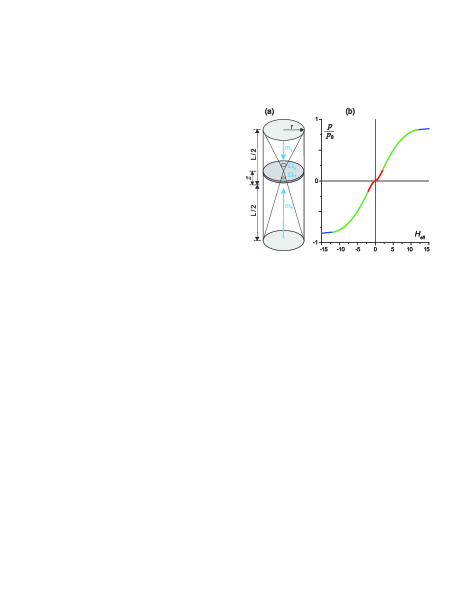
Figure 6: (a) Proposed magnetic domain structure of the wire, where a propagating domain wall separates two domains with antiparallel oriented magnetizations. (b) Dependence of the pressure term as a function of the effective field. The three sub-domains described in text are emphasized with different colors. In the case of a uniform motion of the wall, its constant velocity is proportional with the pressure term.

To model the experimental results in a simple way, we assume that the magnetization processes in these cylindrical wires consist in the displacement of a $180^{\circ}$ domain wall along the entire length of the sample, the wall remaining plane and perpendicular to the cylinder’s axis during its motion, as shown Fig. 6(a). We describe the wall as a two-dimensional geometrical surface, which means that we are neglecting the internal wall structure and the wall thickness. The equation of motion of the domain wall is taken on an analogy between the dynamics of the domain wall and the dynamics of a mechanical viscously damped forced oscillator (see, e.g., Refs. Chikazumi, ; Cullity, ; ch.12 Vazquez 2015, ; Zhukov MSE 1997, ; Varga PRL 2005, ; Vasquez PRL 2012, )

$$\sigma\frac{d^{2}z}{dt^{2}}+\beta\frac{dz}{dt}+\alpha z=p,$$ (1)

where $z$ describes the wall’s position [see Fig. 6(a)], $\sigma$ is the equivalent mass of the wall per unit area, $\beta$ is the viscous damping parameter, $\alpha$ is the restoring coefficient, and the term $p$ on the right hand side of the equation represents the pressure acting on the wall, created by the applied field.

When a domain wall moves, a precessional motion of the moments associated with the wall occurs, and as a result, the wall behaves like it possesses a mass, despite the absence of any actual mass displacement. If in the classical Newton’s mechanics the inertial mass of an object (particle) is determined by its resistance to acceleration due to action of an external force, the inertia of a domain wall reflects an influence of deformations of a moving domain wall on its energy (i.e., how this energy depends on velocity). Doring 1948 A propagating domain wall could continue to propagate, even in the absence of an external magnetic field. The inertia of the wall, or the resistance of the spins to sudden rotation, is not usually important except at very high frequencies.

The second term in the above equation represents a resistance to motion which is proportional to the velocity, and stands for the dissipated energy when the domain wall moves. Three causes of viscous damping have been identified in the scientific literature: production of eddy currents (and consequent Joule heating) around the moving wall, an intrinsic or relaxation effect (arising from the fact that the domain wall velocity is restricted by intrinsic damping of magnetic moments of the domain wall), and a structural relaxation (arising from the interaction of atomic defects with the domain wall). The eddy currents, in turn, produce a magnetic field that acts to oppose the wall motion.

The third term $\alpha z$ represents the restoring force due to crystal imperfections such as microstress or inclusions, $\alpha$ being related to the shape of the potential energy minimum in which the wall is located. The value of $\alpha$ determines the field required to move the wall out of the energy minimum, and the ensemble of $\alpha$ values for the entirely sample determines the coercive field required for extensive wall movement. When the wall moves with the velocity $\upsilon$, the total magnetic moment of the two domains adjacent to the wall changes at the rate $2M_{s}\upsilon$ per unit area of wall, where $M_{s}$ is the wire’s saturation magnetization.

When a magnetic field $H$ is applied parallel to the direction of magnetization of a domain on one side of the wall, the density energy of the system decreases by $2M_{s}H\Delta z$ when the wall is displaced by $\Delta z$, i.e., the term $2M_{s}H$ acts as a pressure on the wall surface. Accordingly, the expression

$$p=2M_{s}H$$ (2)

is commonly used in the scientific literature for the pressure term in the right hand side of the Eq. (1).

Once the wall propagates at the constant velocity $\upsilon_{0}$ under the constant field $H$, then the first term of Eq. (1) drops out because the acceleration is zero, while the third term should be modified because the wall is moving large distances and is not affected by the value of $\alpha$ at one particular energy minimum. Instead, the third term will represent the average resistance to wall motion. In this case from Eqs. (1) and (2) follows that:

$$\upsilon_{0}=\frac{2M_{s}}{\beta}\left(H-H_{c}\right),$$

where $H_{c}$ is the field which should be exceeded before extensive wall motion can occur, and it is approximately equal to the coercive field (or switching field of the axial domain). This linear dependence of the wall velocity on the applied magnetic field is reported in many works, starting with the pioneering work of Sixtus and Tonks in 1931.Sixtus Tonks

However, the velocity of the DW propagation does not increase infinitely, but saturates at some field, the so called Walker limit field.Walker JAP 1974 Above this limit field, the velocity may fluctuate or even oscillates, due to the fact that the spin structure inside the DW is varied by the high magnitude field. On the other hand, when the applied field is smaller than the coercive field the domain wall moves by successive thermally activated jumps. In this low field range it was experimentally found that for thin films the wall’s velocity increases exponentially with the field.Rio-Labrune IEEE 1987 In Ref. Zhukova AIP-CP 2008, is reported that for $\mathrm{Fe}_{69}\mathrm{B}_{15}\mathrm{Si}_{10}\mathrm{C}_{6}$ microwires the dependence $\upsilon_{0}\left(H\right)$ of the velocity on the applied magnetic field is essentially not linear, exhibiting two or three different regimes (depending on the diameter of the wire), with significantly higher domain wall mobility $d\upsilon_{0}\left/dH\right.$ at low field limit. This non linearity was attributed to the change of the DW structure with changing of the applied magnetic field.

This non-linear dependence of the domain wall’s velocity on a constant applied magnetic field is not retrieved from Eqs. (1) and (2). Therefore we propose to introduce the non-linear dependence of the wall velocity in the pressure term from the right hand side of Eq. (1). In the case of a uniform motion of the wall, its constant velocity is proportional to the pressure term. This proportionality suggests the possibility to evaluate the pressure term from the experimental dependence $\upsilon_{0}\left(H\right)$ of the wall velocity as function of the constant field.

In order to find the $\upsilon_{0}\left(H\right)$ dependence for our sample, we have used the same experimental setup as for dFORC measurements, but we have applied a constant magnetic field preceded by a short magnetic field pulse able to initiate the DW depinning. After the initial pulse the wall propagates along the entire microwire under the effect of the constant applied magnetic field. The induced voltage in the detection coils is proportional with the time derivative of the magnetization $dm\left/dt\right.$, i.e., with the wall’s velocity. The procedure was repeated for many values of the constant field to obtain the $\upsilon_{0}\left(H\right)$ dependence. After overcoming the energy barrier corresponding to the DW nucleation and depinning, the DW propagates even in a field smaller than the switching field.

To approximate the experimental data analytically we have used the cumulative distribution function (CDF) of a generalized trapezoidal distribution Dorp Metrica 2003 , because it seems to be appropriate for modeling the duration and the form of a phenomenon which may be represented by two or three stages [see Fig. 6(b)]. In principle, the fitting function is a piece-wise function obtained by concatenating in a continuous manner a power function with a $n_{1}>0$ exponent, a quadratic polynomial, and a power function with a $n_{3}>0$ exponent, the length of each sub-domain being adaptable. Its flexibility allows to appropriately mimic a great variety of behaviors. In our simulations $n_{1}=1.5$ and $n_{3}=3$, respectively.

The effective magnetic field $H_{\mathrm{effective}}=H+H_{i}$ acting on DW, incorporates the applied field and the internal field $H_{i}$. The internal field may contain the demagnetizing field, the anisotropy field, and any other internal field. In order to keep our model simple, in this paper we take into account only the demagnetizing field computed in the middle of the wall, arising from the magnetic uncompensated polarization charges which lie at each end of the cylinder:

$$H_{d} = M_{s}\left(\Omega_{\uparrow}-\Omega_{\downarrow}\right)$$

$$= 2\pi M_{s}\left(\frac{L\left/2\right.+z}{\sqrt{r^{2}+\left(L\left/2\right.+z\right)^{2}}}-\frac{L\left/2\right.-z}{\sqrt{r^{2}+\left(L\left/2\right.-z\right)^{2}}}\right),$$

where $\Omega_{\uparrow}$ and $\Omega_{\downarrow}$ are the solid angles subtended by the cylinder’s bases at the middle of the wall, while $r$ and $L$ are the cylinder’s radius and length, respectively [see Fig. 6(a)]. The demagnetizing field is equal to zero when the wall is in the middle of the wire and its absolue value increases to $2\pi M_{s}L\left/\sqrt{r^{2}+L^{2}}\right.$ as the wall moves to one extremity. Accordingly, the effective field acting on the DW is a function on the wall’s position. The magnetization reversal process depends on the geometry of the magnetic wire through the corresponding variations of demagnetizing field. Of course, the demagnetizing field could be calculated as the average over the wall’s surface. In order to take into account the length of the closure domains, or the critical displacement of the DW to be depinned, in simulations we have taken the maximum value of the DW’s displacement as being $z_{max}\left/\left(L\left/2\right.\right)\right.=0.8$, value given by the normalized magnetization just before the switching on the experimental quasistatic MHL [see Fig. 3(a₁]. The demagnetizing field is oriented so as to saturate the magnetic wire, i.e., the demagnetizing field acts as a pining field of the wall at the ends of the wire. If the sample is saturated, then only a magnetic field with a greater value than that of the demagnetizing field, and acting in opposite direction can start the wall’s motion. However, using the saturation magnetization’s value obtained from the experimental quasistatic MHL, would obtain a switching/pinning field value much greater than the experimental value. This discrepancy is due to the fact that in Eq. (IV) one considered that the magnetic charge density at each end of the wire is equal to the saturation magnetization, i.e., it was considered that there are no closure domain structures at the ends of the wire. The closure domains reduce the total effective magnetic uncompensated charge density, and its value was obtained by the experimental switching field value’s fit.

As we have shown above, the demagnetizing field given by Eq. (IV) is equal to zero in the middle of the wire, otherwise tending to attract the DW towards the nearest end of the wire, its absolute value exhibiting symmetry with respect to the middle of the wire. However, in the experimental dFORCs from Figs. 3(a₁-d₁) and 5(a₁-d₁) we observe that on some dFORCs the moment begins to increase starting from negative values, even if the applied magnetic field is still negative. If we consider that the DW deppined from the upper end of the wire [like in Fig. 6(a)], then this behavior shows that the upper end of the wire still attracts the wall, even if the wall already surpassed the middle of the wire. This comportment can be explained by an asymmetry of the demagnetizing field in regard with the middle of the wire. Such asymmetry can be argued by different densities of magnetic charges on the two ends of the wire. Indeed, if we take into account also the outer shell of the wire, once its magnetization is reversed, the total magnetic charge on the lower end of the wire decreases. Nevertheless, in order to keep our model as simple as possible, in this paper we have considered a symmetric demagnetizing field, as given by Eq. (IV).

As the demagnetizing field includes the field which should be exceeded before extensive wall motion can occur, in the following simulations we have kept only the first two terms in left hand side of Eq. (1), while the pressure function $p\left(H_{\mathrm{effective}}\right)$ from the right hand side is given by the fitting function described above and presented Fig. 6(b).

We have numerically solved this equation and in the following we will show that this simple representation of the domain structure of the magnetic wires is able to explain many peculiarities of their dynamic magnetic behavior. The model, being intrinsically dynamic, is able to predict the magnetization processes, as the sweep rate (or the frequency) of the applied field increases, from the static regime to the dynamical regime. Certainly the above model does not stand for the entire domain structure, but we can interpret our model in terms of a pseudo-wall and two pseudo-domains which overall describe the dynamic magnetization processes of the magnetic wires. Even if the real magnetization process involves complex and intricate domain structures, the above model is a way to reduce the description of the process to few dominant degrees of freedom. We note that Eq. (1) by itself does not contain the physics of nucleation/annihilation of domains, nor the magnetization rotation mechanism, i.e., this model does not deal with the approach to saturation. To describe also these processes, Eq. (1) should be coupled with equations describing the magnetization processes of the outer shell and of the closure domains. Nevertheless, in this paper we neglect these processes. Obviously, full micromagnetic models can better describe the non-uniform magnetization processes, but their numerical efficiency is significantly lower, and this is the reason why the phenomenological models are still used in simulations.

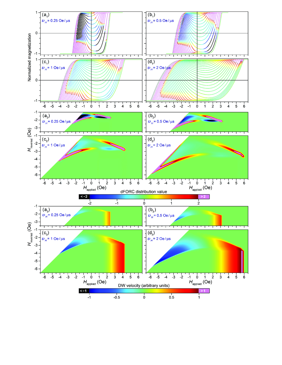
Figure 7: Simulated normalized dFORCs (a₁-d₁), dFORC diagrams (a₂-d₂), and domain wall velocity (a₃-d₃) for different values of the applied field sweep rate $\upsilon_{H}$. The gray curves from dFORCs represent the portions corresponding to a decreasing field.

In order to simulate the experimental data, we first numerically generated a series of triangular magnetic field pulses with increasing amplitude, which were then smoothed using a FFT filter, to obtain a rounding of the tips, as it was in the case of the experiment [see Fig. 2(a)].

Starting from the positive saturation, the DW starts to move only when the decreasing effective magnetic field become negative, i.e., when the applied field overwhelms the threshold value of the pinning field (which, as has been shown above, it is given by the demagnetizing field at the wire’s end). After that, the DW accelerates, the total magnetic moment of the wire being proportional to the wall’s position $z$. After the applied magnetic field reached the appropriate reversal value and started to increase, as long as the effective field is negative, the pressure acting on the wall surface attempts to move it towards the lower end of the wire, and consequently the DW continues to move accelerated toward the lower end. Accordingly, the wire’s magnetic moment continues to decrease even after the applied magnetic field starts to increase. Furthermore, because the DW has inertia, it continues to move down even for positive values of the pressure/effective field. This lag depends on the mass of the wall $\sigma$, on damping $\beta$, and on sweep rate $\upsilon_{H}$. As $\upsilon_{H}$ increases, the lag increases as well, and goes to zero as $\upsilon_{H}$ decreases. Considering a linear pressure term like in Eq. (2) and a sinusoidal excitation, then the driving angular frequency at which the lag of steady-state forced oscillations is maximum (i.e., at phase resonance) is $\omega_{0}=\beta\left/\sigma\right.$.

Systematic simulations have shown that as the $p_{0}\left/\sigma\right.$ ratio increases, the coercive field of dMHL decreases, while the slope $dm_{\mathrm{dMHL}}\left/dH\right.$ increases. As the driving pressure $p_{0}$ exerted on DW increases (and accordingly the force pushing the wall increases), the DW would move faster, with a higher acceleration, and a shorter time would be required for propagation along the wire. A similar effect has the decrease of $\sigma$ because the smaller the mass, the larger the acceleration for a given force. As the damping $\beta$ increases, the acceleration decreases, the time required for propagation along the wire increases, and consequently the coercive field increases, while the slope $dm_{\mathrm{dMHL}}\left/dH\right.$ decreases.

In our simulations $\beta\left/\sigma\right.=1.5\,\mathrm{MHz}$ and $p_{0}\left/\sigma\right.=2\times 10^{10}\,\mathrm{N}\left/\mathrm{m}^{2}\right.$, values that led to a good approximation of the experimental data, both dMHLs and dFORCs (see Fig. 7). Because Eq. (1) does not describe the slowing and stopping of DW at the ends of the wire, the value of the damping was gradually increased as $\left|z\right|>0.7\,z_{\max}$ when DW moves toward the wire’s end. The double-peak structure of the experimental induced voltage [see Fig. 2(a)] could be explained by the existence of pinning centers along the microwire which determine the wall’s deceleration.

The dynamic susceptibility, which is the slope of the magnetization curves, can be written as $\chi_{\mathrm{differerntial}}=dm\left/dH_{\mathrm{applied}}\right.=\left(dm\left/dt\right.\right)\left(dH_{\mathrm{applied}}\left/dt\right.\right)\sim\left(dz\left/dt\right.\right)\left/\upsilon_{H}\right.$, i.e., it is proportional with DW’s velocity.

This fact makes the differential susceptibility diagram (first derivative of the FORCs) probably easier to understand by the potential users of this experimental setup. On this diagram one observes directly the wall velocity. One sees on a typical FORC (e.g., for an initial velocity along the negative direction – given by a value of the reversal field) how the DW is reacting to the field increase at a constant rate from the initial value of the reversal field towards the positive saturation of the wire. The experimental diagram shows at what field the wall is motionless (zero susceptibility on the respective FORC) and how the DW is increasing its positive velocity when the applied field is in the positive region. At very high values of the positive applied field the DW is again motionless at the end of the wire – again the susceptibility is zero on the FORC. As we can make experiments at different field rates one may also observe the inertial effects on DW movements. On these experimental data one have found in some cases a remarkable behavior of the DW (acceleration towards positive direction in negative applied fields) that may suggest in our opinion a brake of symmetry in the unsaturated polarization charges at the two ends of the wire due to a core-shell DW structure. We also would like to emphasis that most of the experimental effects can be covered by the simple model we have proposed.

The classical FORC diagram, which is a second order derivative of the FORCs is offering another aspect of the DW mobility. With the usual unique sensitivity, the FORC diagram is giving details on the coercivities involved in the wire moment switching. The region near the reversal field is quite complicated and offers information about the process of reversal and provides evidence of possible random sources of coercivity like small irregularities in the wire geometrical or physical properties. The second region which covers usually the positive field area on the diagram has a typical structure with a doublet structure: negative for lower reversal fields and positive at higher reversal fields. Our simple model is giving this doublet structure but one may observe that in experiment the angle between the positive and negative regions is significantly lower than in the simulations. As the mentioned structure is closely related to the magnetization processes near saturation we recognize the need for testing more realistic terms for the approach to saturation as it is generally known that the closure structure can be quite intricate. We also see in experimental FORCs evidence of the influence of the shell wall which was neglected in the model. A model with a core-shell structure for the wire would be a logical extension of the model presented in the present article. Also one envisage for a further study experiments with longer wires to test the role of the closure domain wall structure.

V Conclusions

In this article we have introduced a systematic study of kinetic dominated hysteretic processes based on the FORC diagram methodology (dynamic FORC). We propose a number of experiments able to evidence the role of kinetics in the actual hysteretic processes observed in magnetic wires. We have discussed in this article actually two experimental diagrams based on FORC data: (i) the FORC susceptibility diagram is offering a direct image of the DW velocity during the magnetization process along the different FORCs characterized by distinct values of the reversal fields; (ii) the classical FORC diagram calculated as the mixed second order derivative of the FORC data as a function of the reversal and actual applied fields, that gives a supplementary insight on the distribution of coercivities in the system due to various physical causes. The exceptional sensitivity of the FORC diagram method evidenced a number of typical alterations of the quasi-static FORC distribution for a magnetic wire when the field rate is increased. In order to provide the study with a quantitative attribute we have developed a model able to describe rather accurately the entire set of data (dFORC diagrams as a function of field rate and the waiting time in the reversal point). The simple model presented here is in the same time of notable simplicity and still is able to describe in a coherent manner the complexity of the experimental data sets. We also mention the fact that we introduce a methodology for characterizing rate dependent hysteretic processes with the FORC diagram technique, which was used mostly for systems and experiments in which the field rate influence was neglected even in cases in which this effect can’t be avoided and has a strong effect on the switching processes. As many applications of the magnetic wires are dependent on the fast switchings of the magnetization, we expect that this type of experiment to be extensively used by researchers in order to observe systematically how these processes are influenced by various physical parameters. This study opens at least two new lines of research, one centered on the experimental dynamic FORCs and the numerical treatment of experimental data and the second on the model of the domain wall movement which can be dramatically improved in order to include other elements that we have neglected in order to maintain the clarity in a limited space of an article. We already have identified elements from the FORC diagrams that can be correlated to physical parameters of the wall movement (e.g., wall speed limit versus field) and we are very confident that this method could become a valuable tool to obtain important physical information about the dynamic magnetization processes in a variety of magnetic wires and possibly be extended to other magnetic systems.

VI Acknowledgments

Work was supported by Romanian CNCS-UEFISCDI Grants No. PN-II-RU-TE-2012-3-0439 and No. PN-II-RU-TE-2012-3-0449.

References

- (1) F. Preisach, Z. Phys. 94, 277 (1935).
- (2) I. D. Mayergoyz, J. Appl. Phys. 57, 3803 (1985)
- (3) C. R. Pike, A. P. Roberts, and K. L. Verosub, J. Appl. Phys. 85, 6660 (1999).
- (4) A. Stancu, C. Pike, L. Stoleriu, P. Postolache, and D. Cimpoesu, J. Appl. Phys. 93, 6620 (2003).
- (5) E. Della Torre, J. Appl. Phys. 36, 518 (1965).
- (6) C. I. Dobrota and A. Stancu, J. Appl. Phys. 113, 043928 (2013).
- (7) C. I. Dobrota and A. Stancu, Physica B 457, 280 (2015).
- (8) M. Nica and A. Stancu, Physica B 475, 73 (2015).
- (9) A. Stancu, D. Ricinschi, L. Mitoseriu, P. Postolache, and M. Okuyama, Appl. Phys. Lett. 83, 3767 (2003).
- (10) R. Tanasa, C. Enachescu, A. Stancu, J. Linares, E. Codjovi, F. Varret, and J. Haasnoot, Phys. Rev. B 71, 014431 (2005).
- (11) C. Enachescu, R. Tanasa, A. Stancu, F. Varret, J. Linares, and E. Codjovi, Phys. Rev. B 72, 054413 (2005).
- (12) A. Rotaru, J.-H. Lim, D. Lenormand, A. Diaconu, J. B. Wiley, P. Postolache, A. Stancu, and L. Spinu, Phys. Rev. B 84, 134431 (2011).
- (13) X. Kou, X. Fan, R. K. Dumas, Q. Lu, Y. Zhang, H. Zhu, X. Zhang, K. Liu, and J. Q. Xiao, Adv. Mater. 23, 1393 (2011).
- (14) R. Street and J. C. Woolley, Proc. Phys. Soc., London, Sect. A 62, 562 (1949); Proc. Phys. Soc. London, Sect. B 63, 509 (1950).
- (15) L. Néel, J. Phys. Radium 11, 49 (1950); J. Phys. Radium 12, 339 (1951).
- (16) Magnetic Nano- and Microwires: Design, Synthesis, Properties and Applications, Edited by Manuel Vásquez (Elsevier Science and Technology, Cambridge, UK, 2015)
- (17) L. Spinu, A. Stancu, C. Radu, F. Li, and J. B. Wiley, IEEE Trans. Magn. 40, 2116 (2004).
- (18) L. Clime, T. Veres, A. Yelon, J. Appl. Phys. 102, 013903 (2007).
- (19) F. Beron, L. P. Carignan, D. Menard, and A. Yelon, Chapter 7 in Electrodeposited Nanowires and their Applications (InTechECH, Croatia, 2010)
- (20) M. P. Proenca, K. J. Merazzo, L. G. Vivas, D. C. Leitao, C. T. Sousa, J. Ventura, J. P. Araujo, and M. Vázquez, Nanotechnology 24, 475703 (2013).
- (21) M. Almasi-Kashi, A. Ramazani, and M. Amiri-Dooreh, Physica B 452, 124 (2014).
- (22) Pavel Ripka, Magnetic Sensors and Magnetometers (Artech House Publishers, Norwood, United States, 2001)
- (23) F. Beron, G. Soares, and K. R. Pirota, Rev. Sci. Instrum. 82, 063904 (2011).
- (24) A. Zhukov and V. Zhukova, Magnetic Properties and Applications of Ferromagnetic Microwires with Amorphous and Nanocrystalline Structure, p. 11788 (Nova Science, vol. 162, 2009, Hauppauge, NY).
- (25) M. Ipatov, V. Zhukova, A. K. Zvezdin, and A. Zhukov, J. Appl. Phys. 106, 103902 (2009).
- (26) R. Varga, K. L. Garcia, M. Vázquez, and P. Vojtanik, Phys. Rev. Lett. 94, 017201 (2005).
- (27) M. Vázquez, G. A. Basheed, G. Infante, and R. P. Del Real, Phys. Rev. Lett. 108, 037201(2012).
- (28) J. Ye, R. P. del Real, G. Infante, and M. Vázquez, J. Appl. Phys. 113, 043904 (2013).
- (29) V. Zhukova, J. M. Blanco, V. Rodionova, M. Ipatov, and A. Zhukov, Journal of Alloys and Compounds 586 S287 (2014).
- (30) T. A. Óvári, N. Lupu, and H. Chiriac, Rapidly Solidified Magnetic Nanowires and Submicron Wires, Chapter 1 in Advanced Magnetic Materials (InTechECH, Croatia, 2010)
- (31) S. Corodeanu, H. Chiriac, and T. A. Óvári, Rev. Sci. Instrum. 82, 094701 (2011).
- (32) http://earthref.org/FORCinel
- (33) A. Rotaru, F. Varret, A. Gindulescu, J. Linares, A. Stancu, J. F. Letard, T. Forestier, C. Etrillard, Eur. Phys. J. B 84, 439 (2011).
- (34) M. Vázquez, A. Jimenez, and R. Perez del Real, Controlled single-domain wall motion in cylindrical magnetic microwires with axial anisotropy, Chapter 12 of Ref. Vazquez 2015,
- (35) A. Zhukov, M. Vázquez, J. Velazquez, C. Garcia, R. Valenzuela, and B. Ponomarev, Materials Science and Engineering A 226-228, 753 (1997).
- (36) S. Chikazumi, Physics of Ferromagnetism (Clarendon Press, Oxford, 1997), p. 575.
- (37) B. D. Cullity and C. D. Graham, Introduction to magnetic materials (Wiley-IEEE Press, 2009), p. 412.
- (38) W. Döring, Z. Naturforsch. 3a, 373 (1948).
- (39) K. J. Sixtus and L. Tonks, Phys. Rev. 37, 930 (1931).
- (40) N. L. Schryer and L. R. Walker, J. Appl. Phys. 45, 5406 (1974).
- (41) F. Rio, P. Bernstein, and M. Labrune, IEEE Trans. Magn. Mag. 23, 2266 (1987).
- (42) V. Zhukova, J. M. Blanco, M. Ipatov, J. Gonzalez, and A. Zhukov, AIP Conference Proceedings 1003, 301 (2008)
- (43) J. R. Dorp and S. Kotz, Metrica 58, 85 (2003)