Recursive nonlinear-system identification using latent variables

Abstract

In this paper we develop a method for learning nonlinear system models with multiple outputs and inputs. We begin by modelling the errors of a nominal predictor of the system using a latent variable framework. Then using the maximum likelihood principle we derive a criterion for learning the model. The resulting optimization problem is tackled using a majorization-minimization approach. Finally, we develop a convex majorization technique and show that it enables a recursive identification method. The method learns parsimonious predictive models and is tested on both synthetic and real nonlinear systems.

I Introduction

In this paper we consider the problem of learning a nonlinear dynamical system model with multiple outputs $\mathbf{y}(t)$ and multiple inputs $\mathbf{u}(t)$ (when they exist). Generally this identification problem can be tackled using different model structures, with the class of linear models being arguably the most well studied in engineering, statistics and econometrics [27, 15, 6, 2, 7].

Linear models are often used even when the system is known to be nonlinear [10, 25]. However certain nonlinearities, such as saturations, cannot always be neglected. In such cases using block-oriented models is a popular approach to capture static nonlinearities [11]. Recently, such models have been given semiparametric formulations and identified using machine learning methods, cf. [22, 23]. To model nonlinear dynamics a common approach is to use Narmax models [26, 5].

In this paper we are interested in recursive identification methods [18]. In cases where the model structure is linear in the parameters, recursive least-squares can be applied. For certain models with nonlinear parameters, the extended recursive least-squares has been used [8]. Another popular approach is the recursive prediction error method which has been developed, e.g., for Wiener models, Hammerstein models, and polynomial state-space models [33, 19, 31].

Nonparametric models are often based on weighted sums of the observed data [24]. The weights vary for each predicted output and the number of weights increases with each observed datapoint. The weights are typically obtained in a batch manner; in [1, 4] they are computed recursively but must be recomputed for each new prediction of the output.

For many nonlinear systems, however, linear models work well as an initial approximation. The strategy in [21] exploits this fact by first finding the best linear approximation using a frequency domain approach. Then, starting from this approximation, a nonlinear polynomial state-space model is fitted by solving a nonconvex problem. This two-step method cannot be readily implemented recursively and it requires input signals with appropriate frequency domain properties.

In this paper, we start from a nominal model structure. This class can be based on insights about the system, e.g. that linear model structures can approximate a system around an operating point. Given a record of past outputs, $\mathbf{y}(t)$ and inputs $\mathbf{u}(t)$, that is,

$$\mathcal{D}_{t}\triangleq\bigl{\{}\;\left(\mathbf{y}(1),\mathbf{u}(1)\right),\dots,\left(\mathbf{y}(t),\mathbf{u}(t)\right)\;\bigr{\}},$$

a nominal model yields a predicted output $\mathbf{y}_{0}(t+1)$ which differs from the output $\mathbf{y}(t+1)$. The resulting prediction error is denoted $\boldsymbol{\varepsilon}(t+1)$ [16]. By characterizing the nominal prediction errors in a data-driven manner, we aim to develop a refined predictor model of the system. Thus we integrate classic and data-driven system modeling approaches in a natural way.

The general model class and problem formulation are introduced in Section II. Then in Section III we apply the principle of maximum likelihood to derive a statistically motivated learning criterion. In Section IV this nonconvex criterion is minimized using a majorization-minimization approach that gives rise to a convex user-parameter free method. We derive a computionally efficient recursive algorithm for solving the convex problem, which can be applied to large datasets as well as online learning scenarios. In Section V, we evaluate the proposed method using both synthetic and real data examples.

In a nutshell, the contribution of the paper is a modelling approach and identification method for nonlinear multiple input-multiple output systems that:

• explicitly separates modeling based on application-specific insights from general data-driven modelling,

• circumvents the choice of regularization parameters and initialization points,

• learns parsimonious predictor models,

• admits a computationally efficient implementation.

Notation: $\mathbf{E}_{i,j}$ denotes the $ij$th standard basis matrix. $\otimes$ and $\odot$ denote the Kronecker and Hadamard products, respectively. $\text{vec}(\cdot)$ is the vectorization operation. $\|\mathbf{x}\|_{2}$, $\|\mathbf{x}\|_{1}$ and $\|\mathbf{X}\|_{\mathbf{W}}=\sqrt{\text{tr}\{\mathbf{X}^{\top}\mathbf{W}\mathbf{X}\}}$, where $\mathbf{W}\succ\mathbf{0}$, denote $\ell_{2}$-, $\ell_{1}$- and weighted norms, respectively. The Moore-Penrose pseudoinverse of $\mathbf{X}$ is denoted $\mathbf{X}^{\dagger}$.

Remark 1.

An implementation of the proposed method is available at https://github.com/magni84/lava.

II Problem formulation

Given $\mathcal{D}_{t-1}$, the $n_{y}$-dimensional output of a system can always be written as

$$\mathbf{y}(t)=\mathbf{y}_{0}(t)+\boldsymbol{\varepsilon}(t),$$ (1)

where $\mathbf{y}_{0}(t)$ is any one-step-ahead predictor based on a nominal model. Here we consider nominal models on the form

$$\mathbf{y}_{0}(t)=\boldsymbol{\Theta}\boldsymbol{\varphi}(t),$$ (2)

where the $p\times 1$ vector $\boldsymbol{\varphi}(t)$ is a given function of $\mathcal{D}_{t-1}$ and $\boldsymbol{\Theta}$ denotes the unknown parameters.

Remark 2.

A typical example of $\boldsymbol{\varphi}(t)$ is

$$\boldsymbol{\varphi}(t)=[\mathbf{y}^{\top}(t-1)\>\cdots\>\mathbf{y}^{\top}(t-n_{a})\;\mathbf{u}^{\top}(t-1)\>\cdots\>\mathbf{u}^{\top}(t-n_{b})\;1]^{\top},$$ (3)

in which case the nominal predictor is linear in the data and therefore captures the linear system dynamics. Nonlinearities can be incorporated if such are known about the system, in which case $\boldsymbol{\varphi}(t)$ will be nonlinear in the data.

The popular Arx model structure, for instance, can be cast into the framework (1) and (2) by assuming that the nominal prediction error $\boldsymbol{\varepsilon}(t)$ is a white noise process [27, 15]. For certain systems, (2) may accurately describe the dynamics of the system around its operation point and consequently the white noise assumption on $\boldsymbol{\varepsilon}(t)$ may be a reasonable approximation. However, this ceases to be the case even for systems with weak nonlinearities, cf. [10].

Next, we develop a data-driven model of the prediction errors $\boldsymbol{\varepsilon}(t)$ in (1), conditioned on the past data $\mathcal{D}_{t-1}$. Specifically, we assume the conditional model

$$\boldsymbol{\varepsilon}(t)\>|\>\mathcal{D}_{t-1}\;\sim\;\mathcal{N}(\mathbf{Z}\boldsymbol{\gamma}(t),\boldsymbol{\Sigma}),$$ (4)

where $\mathbf{Z}$ is an $n_{y}\times q$ matrix of unknown latent variables, $\boldsymbol{\Sigma}$ is an unknown covariance matrix, and the $q\times 1$ vector $\boldsymbol{\gamma}(t)$ is any given function of $\mathcal{D}_{t-1}$. This is a fairly general model structure that can capture correlated data-dependent nominal prediction errors.

Note that when $\mathbf{Z}\equiv\mathbf{0}$, the prediction errors are temporally white and the nominal model (2) captures all relevant system dynamics. The latent variable is modeled as random here. Before data collection, we assume $\mathbf{Z}$ to have mean $\mathbf{0}$ as we have no reason to depart from the nominal model assumptions until after observing data. Using a Gaussian distribution, we thus get

$$\operatorname{vec}(\mathbf{Z})\sim\mathcal{N}(\mathbf{0},\mathbf{D}),$$ (5)

where $\mathbf{D}$ is an unknown covariance matrix.

Our goal here is to identify a refined predictor of the form

$$\boxed{\hat{\mathbf{y}}(t)=\underbrace{\widehat{\boldsymbol{\Theta}}\boldsymbol{\varphi}(t)}_{\hat{\mathbf{y}}_{0}(t)}+\underbrace{\widehat{\mathbf{Z}}\boldsymbol{\gamma}(t)}_{\hat{\boldsymbol{\varepsilon}}(t)},}$$ (6)

from a data set $\mathcal{D}_{t-1}$, by maximizing the likelihood function. The first term is an estimate of the nominal predictor model while the second term tries to capture structure in the data that is not taken into account by the nominal model. Note that when $\widehat{\mathbf{Z}}$ is sparse we obtain a parsimonious predictor model.

Remark 3.

The model (1)-(4) implies that we can write the output in the equivalent form

$$\mathbf{y}(t)=\boldsymbol{\Theta}\boldsymbol{\varphi}(t)+\mathbf{Z}\boldsymbol{\gamma}(t)+\mathbf{v}(t),$$

where $\mathbf{v}(t)$ is a white process with covariance $\boldsymbol{\Sigma}$. In order to formulate a flexible data-driven error model (4), we overparametrize it using a high-dimensional $\boldsymbol{\gamma}(t)$. In this case, regularization of $\mathbf{Z}$ is desirable, which is achieved by (5). Note that $\mathbf{D}$ and $\boldsymbol{\Sigma}$ are both unknown. Estimating these covariance matrices corresponds to using a data-adaptive regularization, as we show in subsequent sections.

Remark 4.

The nonlinear function $\boldsymbol{\gamma}(t)$ of $\mathcal{D}_{t-1}$ can be seen as a basis expansion which is chosen to yield a flexible model structure of the errors. In the examples below we will use the Laplace operator basis functions [28]. Other possible choices include the polynomial basis functions, Fourier basis functions, wavelets, etc. [26, 15, 32].

Remark 5.

In (6), $\hat{\mathbf{y}}(t)$ is a one-step-ahead predictor. However, the framework can be readily applied to $k$-step-ahead prediction where $\boldsymbol{\varphi}(t)$ and $\boldsymbol{\gamma}(t)$ depend on $\mathbf{y}(1),\dots,\mathbf{y}(t-k)$.

III Latent variable framework

Given a record of $N$ data samples, $\mathcal{D}_{N}$, our goal is to estimate $\boldsymbol{\Theta}$ and $\mathbf{Z}$ to form the refined predictor (6). In Section III-A, we employ the maximum likelihood approach based on the likelihood function $p(\mathbf{Y}|\boldsymbol{\Theta},\mathbf{D},\boldsymbol{\Sigma})$, which requires the estimation of nuisance parameters $\mathbf{D}$ and $\boldsymbol{\Sigma}$. For notational simplicity, we write the parameters as $\boldsymbol{\Omega}=\{\boldsymbol{\Theta},\mathbf{D},\boldsymbol{\Sigma}\}$ and in Section III-B we show how an estimator of $\mathbf{Z}$ is obtained as a function of $\boldsymbol{\Omega}$ and $\mathcal{D}_{N}$.

III-A Parameter estimation

We write the output samples in matrix form as

$$\mathbf{Y}=\begin{bmatrix}\mathbf{y}(1)&\cdots&\mathbf{y}(N)\end{bmatrix}\in\mathbb{R}^{n_{y}\times N}.$$

In order to obtain maximum likelihood estimates of $\boldsymbol{\Omega}$, we first derive the likelihood function by marginalizing out the latent variables from the data distribution:

$$p(\mathbf{Y}|\boldsymbol{\Omega})=\int p(\mathbf{Y}|\boldsymbol{\Omega},\mathbf{Z})p(\mathbf{Z})d\mathbf{Z},$$ (7)

where the data distribution $p(\mathbf{Y}|\boldsymbol{\Omega},\mathbf{Z})$ and $p(\mathbf{Z})$ are given by (4) and (5), respectively.

To obtain a closed-form expression of (7), we begin by constructing the regression matrices

$$\boldsymbol{\Phi} =\begin{bmatrix}\boldsymbol{\varphi}(1)&\cdots&\boldsymbol{\varphi}(N)\end{bmatrix}\in\mathbb{R}^{p\times N},$$

$$\boldsymbol{\Gamma} =\begin{bmatrix}\boldsymbol{\gamma}(1)&\cdots&\boldsymbol{\gamma}(N)\end{bmatrix}\in\mathbb{R}^{q\times N}.$$

It is shown in Appendix A that (7) can be written as

$$p(\mathbf{Y}|\boldsymbol{\Omega})=\frac{1}{(2\pi)^{Nn_{y}}|\mathbf{R}|}\exp\left(-\frac{1}{2}\|\mathbf{y}-\mathbf{F}\boldsymbol{\theta}\|^{2}_{\mathbf{R}^{-1}}\right),$$ (8)

where

$$\mathbf{y}=\operatorname{vec}(\mathbf{Y}),\quad\boldsymbol{\theta}=\operatorname{vec}(\boldsymbol{\Theta}),\quad\mathbf{z}=\operatorname{vec}(\mathbf{Z}),$$ (9)

are vectorized variables, and

$$\mathbf{F} =\boldsymbol{\Phi}^{\top}\otimes\mathbf{I}_{n_{y}},\quad\mathbf{G}=\boldsymbol{\Gamma}^{\top}\otimes\mathbf{I}_{n_{y}},$$ (10)

$$\mathbf{R} \triangleq\mathbf{G}\mathbf{D}\mathbf{G}^{\top}+\mathbf{I}_{N}\otimes\boldsymbol{\Sigma}.$$ (11)

Note that (8) is not a Gaussian distribution in general, since $\mathbf{R}$ may be a function of $\mathbf{Y}$. It follows that maximizing (8) is equivalent to solving

$$\min_{\boldsymbol{\Omega}}\;V(\boldsymbol{\Omega}),$$ (12)

where

$$\boxed{V(\boldsymbol{\Omega})\triangleq\|\mathbf{y}-\mathbf{F}\boldsymbol{\theta}\|^{2}_{\mathbf{R}^{-1}}+\ln|\mathbf{R}|}$$ (13)

and $\mathbf{y}-\mathbf{F}\boldsymbol{\theta}=\operatorname{vec}(\mathbf{Y}-\boldsymbol{\Theta}\boldsymbol{\Phi})=\operatorname{vec}([\boldsymbol{\varepsilon}(1)\>\cdots\>\boldsymbol{\varepsilon}(N)])$ is nothing but the vector of nominal prediction errors.

III-B Latent variable estimation

Next, we turn to the latent variable $\mathbf{Z}$ which is used to model the nominal prediction error $\boldsymbol{\varepsilon}(t)$ in (4). As we show in Appendix A, the conditional distribution of $\mathbf{Z}$ is Gaussian and can be written as

$$p(\mathbf{Z}|\boldsymbol{\Omega},\mathbf{Y})=\frac{1}{\sqrt{(2\pi)^{n_{y}q}|\mathbf{\Sigma}_{z}|}}\exp\left(-\frac{1}{2}\|\mathbf{z}-\boldsymbol{\zeta}\|_{\mathbf{\Sigma}_{z}^{-1}}^{2}\right),$$ (14)

with conditional mean

$$\boldsymbol{\zeta}=\mathbf{D}\mathbf{G}^{\top}\mathbf{R}^{-1}(\mathbf{y}-\mathbf{F}\boldsymbol{\theta}),$$ (15)

and covariance matrix

$$\mathbf{\Sigma}_{z}=\left(\mathbf{D}^{-1}+\mathbf{G}^{\top}(\mathbf{I}_{N}\otimes\boldsymbol{\Sigma}^{-1})\mathbf{G}\right)^{-1}.$$ (16)

An estimate $\widehat{\mathbf{Z}}$ is then given by evaluating the conditional (vectorized) mean (15) at the optimal estimate $\widehat{\boldsymbol{\Omega}}$ obtained via (12).

IV Majorization-minimization approach

The quantities in the refined predictor (6) are readily obtained from the solution of (12). In general, $V(\boldsymbol{\Omega})$ may have local minima and (12) must be tackled using computationally efficient iterative methods to find the optimum. The obtained estimates will then depend on the choice of initial point $\boldsymbol{\Omega}_{0}$. Such methods includes the majorization-minimization approach [12, 35], which in turn include Expectation Maximization [9] as a special case.

The majorization-minimization approach is based on finding a majorizing function $V^{\prime}(\boldsymbol{\Omega}|\widetilde{\boldsymbol{\Omega}})$ with the following properties:

$$V(\boldsymbol{\Omega})\leq V^{\prime}(\boldsymbol{\Omega}|\widetilde{\boldsymbol{\Omega}}),\quad\forall\boldsymbol{\Omega}$$ (17)

with equality when $\boldsymbol{\Omega}=\widetilde{\boldsymbol{\Omega}}$. The key is to find a majorizing function that is simpler to minimize than $V(\boldsymbol{\Omega})$. Let $\boldsymbol{\Omega}_{k+1}$ denote the minimizer of $V^{\prime}(\boldsymbol{\Omega}|\boldsymbol{\Omega}_{k})$. Then

$$\begin{split}V(\boldsymbol{\Omega}_{k+1})&\leq V^{\prime}(\boldsymbol{\Omega}_{k+1}|\boldsymbol{\Omega}_{k})\leq V^{\prime}(\boldsymbol{\Omega}_{k}|\boldsymbol{\Omega}_{k})=V(\boldsymbol{\Omega}_{k}).\end{split}$$ (18)

This property leads directly to an iterative scheme that decreases $V(\boldsymbol{\Omega})$ monotonically, starting from an initial estimate $\boldsymbol{\Omega}_{0}$.

Given the overparameterized error model (4), it is natural to initialize at points in the parameter space which correspond to the nominal predictor model structure (2). That is,

$$\boldsymbol{\Omega}_{0}=\{\boldsymbol{\Theta}_{0},\mathbf{0},\boldsymbol{\Sigma}_{0}\},\qquad\text{where}\quad\boldsymbol{\Sigma}_{0}\succ\mathbf{0},$$ (19)

at which $\widehat{\mathbf{Z}}\equiv\mathbf{0}$.

IV-A Convex majorization

For a parsimonious parameterization and computationally advantageous formulation, we consider a diagonal structure of the covariance matrices in (4), i.e., we let

$$\boldsymbol{\Sigma}=\text{diag}(\sigma_{1},\sigma_{2},\dots,\sigma_{n_{y}}),$$ (20)

and we let $\mathbf{D}_{i}=\text{diag}(d_{i,1},\ldots,d_{i,q})$ denote the covariance matrix corresponding to the $i$th row of $\mathbf{Z}$, so that

$$\mathbf{D}=\sum_{i=1}^{n_{y}}\mathbf{D}_{i}\otimes\mathbf{E}_{i,i}.$$ (21)

We begin by majorizing (13) via linearization of the concave term $\ln|\mathbf{R}|$:

$$\begin{split}\ln|\mathbf{R}|&\leq\ln|\widetilde{\mathbf{R}}|-\operatorname{tr}\{\widetilde{\mathbf{R}}^{-1}(\mathbf{I}_{N}\otimes\widetilde{\boldsymbol{\Sigma}})\}-\operatorname{tr}\{\mathbf{G}^{\top}\widetilde{\mathbf{R}}^{-1}\mathbf{G}\widetilde{\mathbf{D}}\}\\ &\quad+\operatorname{tr}\{\widetilde{\mathbf{R}}^{-1}(\mathbf{I}_{N}\otimes\boldsymbol{\Sigma})\}+\operatorname{tr}\{\mathbf{G}^{\top}\widetilde{\mathbf{R}}^{-1}\mathbf{G}\mathbf{D}\},\end{split}$$ (22)

where $\widetilde{\mathbf{D}}$ and $\widetilde{\boldsymbol{\Sigma}}$ are arbitrary diagonal covariance matrices and $\widetilde{\mathbf{R}}$ is obtained by inserting $\widetilde{\mathbf{D}}$ and $\widetilde{\boldsymbol{\Sigma}}$ into (11). The right-hand side of the inequality above is a majorizing tangent plane to $\ln|\mathbf{R}|$, see Appendix B. The use of (22) yields a convex majorizing function of $V(\boldsymbol{\Omega})$ in (12):

$$\begin{split}V^{\prime}(\boldsymbol{\Omega}|\widetilde{\boldsymbol{\Omega}})&=\|\mathbf{y}-\mathbf{F}\boldsymbol{\theta}\|^{2}_{\mathbf{R}^{-1}}+\operatorname{tr}\{\widetilde{\mathbf{R}}^{-1}(\mathbf{I}_{N}\otimes\boldsymbol{\Sigma})\}\\ &\quad+\operatorname{tr}\{\mathbf{G}^{\top}\widetilde{\mathbf{R}}^{-1}\mathbf{G}\mathbf{D}\}+\widetilde{K},\end{split}$$ (23)

where $\widetilde{K}=\ln|\widetilde{\mathbf{R}}|-\operatorname{tr}\{\widetilde{\mathbf{R}}^{-1}(\mathbf{I}_{N}\otimes\widetilde{\boldsymbol{\Sigma}})\}-\operatorname{tr}\{\mathbf{G}^{\top}\widetilde{\mathbf{R}}^{-1}\mathbf{G}\widetilde{\mathbf{D}}\}$ is a constant. To derive a computationally efficient algorithm for minimizing (23), the following theorem is useful:

Theorem 1.

The majorizing function (23) can also be written as

$$V^{\prime}(\boldsymbol{\Omega}|\widetilde{\boldsymbol{\Omega}})=\min_{\mathbf{Z}}\;V^{\prime}(\boldsymbol{\Omega}|\mathbf{Z},\widetilde{\boldsymbol{\Omega}})$$ (24)

where

$$\begin{split}V^{\prime}(\boldsymbol{\Omega}|\mathbf{Z},\widetilde{\boldsymbol{\Omega}})&=\|\mathbf{Y}-\boldsymbol{\Theta}\boldsymbol{\Phi}-\mathbf{Z}\boldsymbol{\Gamma}\|^{2}_{\boldsymbol{\Sigma}^{-1}}+\|\operatorname{vec}(\mathbf{Z})\|_{\mathbf{D}^{-1}}^{2}\\ &\quad+\operatorname{tr}\{\widetilde{\mathbf{R}}^{-1}(\mathbf{I}_{N}\otimes\boldsymbol{\Sigma})\}+\operatorname{tr}\{\mathbf{G}^{\top}\widetilde{\mathbf{R}}^{-1}\mathbf{G}\mathbf{D}\}+\widetilde{K}.\end{split}$$ (25)

The minimizing $\mathbf{Z}$ is given by the conditional mean (15).

Proof.

The problem in (24) has a minimizing $\mathbf{Z}$ which, after vectorization, equals $\boldsymbol{\zeta}$ in (15). Inserting the minimizing $\mathbf{Z}$ into (25) and using (41) yields (23). ∎

Remark 6.

The augmented form in (23), enables us to solve for the nuisance parameters $\mathbf{D}$ and $\boldsymbol{\Sigma}$ in closed-form and also yields the conditional mean $\widehat{\mathbf{Z}}$ as a by-product.

To prepare for the minimization of the function (25) we write the matrix quantities using variables that denote the $i$th rows of the following matrices:

$$\mathbf{Y}=\begin{bmatrix}\vdots\\ \mathbf{y}^{\top}_{i}\\ \vdots\end{bmatrix},\quad\boldsymbol{\Theta}=\begin{bmatrix}\vdots\\ \boldsymbol{\theta}^{\top}_{i}\\ \vdots\end{bmatrix},\quad\mathbf{Z}=\begin{bmatrix}\vdots\\ \mathbf{z}^{\top}_{i}\\ \vdots\end{bmatrix},\quad\boldsymbol{\Gamma}=\begin{bmatrix}\vdots\\ \boldsymbol{\gamma}^{\top}_{i}\\ \vdots\end{bmatrix}.$$

Theorem 2.

After concentrating out the nuisance parameters, the minimizing arguments $\boldsymbol{\Theta}$ and $\mathbf{Z}$ of the function (25) are obtained by solving the following convex problem:

$$\min_{\boldsymbol{\Theta},\mathbf{Z}}\;\sum_{i=1}^{n_{y}}\left(\|\mathbf{y}_{i}-\boldsymbol{\Phi}^{\top}\boldsymbol{\theta}_{i}-\boldsymbol{\Gamma}^{\top}\mathbf{z}_{i}\|_{2}+\|\mathbf{w}_{i}\odot\mathbf{z}_{i}\|_{1}\right)$$ (26)

where

$$\mathbf{w}_{i} =\begin{bmatrix}w_{i,1}&\cdots&w_{i,q}\end{bmatrix}^{\top},\quad w_{i,j}=\sqrt{\frac{{\boldsymbol{\gamma}}_{j}^{\top}\widetilde{\mathbf{R}}_{i}^{-1}{\boldsymbol{\gamma}}_{j}}{\operatorname{tr}\{\widetilde{\mathbf{R}}_{i}^{-1}\}}}$$ (27)

$$\widetilde{\mathbf{R}}_{i} =\boldsymbol{\Gamma}\widetilde{\mathbf{D}}_{i}\boldsymbol{\Gamma}^{\top}+\widetilde{\sigma}_{i}\mathbf{I}_{N}.$$ (28)

The closed-form expression for the minimizing nuisance parameters (20) and (21) are given by

$$\hat{\sigma}_{i} =\frac{\|\mathbf{y}_{i}-\boldsymbol{\Phi}^{\top}\boldsymbol{\theta}_{i}-\boldsymbol{\Gamma}^{\top}\mathbf{z}_{i}\|_{2}}{\sqrt{\operatorname{tr}\{\widetilde{\mathbf{R}}_{i}^{-1}\}}},\,\hat{d}_{i,j}=\frac{|z_{i,j}|}{\sqrt{{\boldsymbol{\gamma}}_{j}^{\top}\widetilde{\mathbf{R}}_{i}^{-1}{\boldsymbol{\gamma}}_{j}}}.$$ (29)

Proof.

See Appendix C. ∎

Remark 7.

Problem (26) contains a data-adaptive regularizing term which typically leads to parsimonious estimates of $\mathbf{Z}$, cf. [30].

Remark 8.

Majorizing at a nominal predictor model, i.e. $\widetilde{\boldsymbol{\Omega}}=\{\widetilde{\boldsymbol{\Theta}},\mathbf{0},\widetilde{\boldsymbol{\Sigma}}\}$ as discussed above, yields $\widetilde{\mathbf{R}}_{i}=\widetilde{\sigma}_{i}\mathbf{I}_{N}$ and the weights are given by

$$w_{i,j}=\frac{\|{\boldsymbol{\gamma}}_{j}\|_{2}}{\sqrt{N}}.$$ (30)

Then problem (26) and consequently the minimization of (24) becomes invariant with respect to $\widetilde{\boldsymbol{\Sigma}}$.

The iterative scheme (18) is executed by initializing at $\widetilde{\boldsymbol{\Omega}}:=\boldsymbol{\Omega}_{0}$ and solving (26). The procedure is then repeated by updating the majorization point using the new estimate $\widetilde{\boldsymbol{\Omega}}:=\widehat{\boldsymbol{\Omega}}$. It follows that the estimates will converge to a local minima of (13). The following theorem establishes that the local minima found, and thus the resulting predictor (6), is invariant to $\boldsymbol{\Omega}_{0}$ in the form (19).

Theorem 3.

All initial points $\boldsymbol{\Omega}_{0}$ in the form (19) result in the same sequence of minimizers $(\widehat{\boldsymbol{\Theta}}_{k},\widehat{\mathbf{Z}}_{k})$ of (26), for all $k>0$. Moreover, the sequence $(\widehat{\mathbf{D}}_{k},\widehat{\boldsymbol{\Sigma}}_{k})$ converges to a unique point when $k\rightarrow\infty$.

Proof.

See Appendix D. ∎

Remark 9.

As a result we may initialize the scheme (18) at $\boldsymbol{\Omega}_{0}=\{\mathbf{0},\mathbf{0},\mathbf{I}_{n_{y}}\}$. This obviates the need for carefully selecting an initialization point, which would be needed in e.g. the Expectation Maximization algorithm.

IV-B Recursive computation

We now show that the convex problem (26) can be solved recursively, for each new sample $\mathbf{y}(t)$ and $\mathbf{u}(t)$.

IV-B1 Computing $\widehat{\boldsymbol{\Theta}}$

If we fix $\mathbf{Z}$ and only solve for $\boldsymbol{\Theta}$, the solution is given by

$$\widehat{\boldsymbol{\Theta}}=\overline{\boldsymbol{\Theta}}-\mathbf{Z}\mathbf{H}^{\top}$$ (31)

where

$$\overline{\boldsymbol{\Theta}}=\mathbf{Y}\boldsymbol{\Phi}^{\dagger}\quad\text{and}\quad\mathbf{H}^{\top}=\boldsymbol{\Gamma}\boldsymbol{\Phi}^{\dagger}.$$

Note that both $\overline{\boldsymbol{\Theta}}$ and $\mathbf{H}$ are independent of $\mathbf{Z}$, and that they can be computed for each sample $t$ using a standard recursive least-squares (LS) algorithm:

$$\overline{\boldsymbol{\Theta}}(t) =\overline{\boldsymbol{\Theta}}(t-1)+(\mathbf{y}(t)-\overline{\boldsymbol{\Theta}}(t-1)\boldsymbol{\varphi}(t))\boldsymbol{\varphi}^{\top}(t)\mathbf{P}(t)$$ (32)

$$\mathbf{H}(t) =\mathbf{H}(t-1)+\mathbf{P}(t)\boldsymbol{\varphi}(t)(\boldsymbol{\gamma}^{\top}(t)-\boldsymbol{\varphi}^{\top}(t)\mathbf{H}(t-1))$$ (33)

$$\mathbf{P}(t) =\mathbf{P}(t-1)-\frac{\mathbf{P}(t-1)\boldsymbol{\varphi}(t)\boldsymbol{\varphi}^{\top}(t)\mathbf{P}(t-1)}{1+\boldsymbol{\varphi}^{\top}(t)\mathbf{P}(t-1)\boldsymbol{\varphi}(t)}.$$ (34)

Remark 10.

Natural initial values are $\overline{\boldsymbol{\Theta}}(0)=\mathbf{0}$ and $\mathbf{H}(0)=\mathbf{0}$. The matrix $\boldsymbol{\Phi}^{\dagger}$ equals $\boldsymbol{\Phi}^{\top}(\boldsymbol{\Phi}\boldsymbol{\Phi}^{\top})^{-1}$ when $t\geq p$ samples yield a full-rank matrix $\boldsymbol{\Phi}$. The matrix $\mathbf{P}(t)$ converges to $(\boldsymbol{\Phi}\boldsymbol{\Phi}^{\top})^{-1}$. A common choice for the initial value of $\mathbf{P}(t)$ is $\mathbf{P}(0)=c\mathbf{I}$, where a larger constant $c>0$ leads to a faster convergence of (34), cf. [27, 29].

IV-B2 Computing $\widehat{\mathbf{Z}}$

Using (31), we concentrate out $\boldsymbol{\Theta}$ from (26) to obtain

$$V^{\prime}(\mathbf{Z})=\sum_{i=1}^{n_{y}}\left(\|\boldsymbol{\xi}_{i}-\left(\boldsymbol{\Gamma}^{\top}-\boldsymbol{\Phi}^{\top}\mathbf{H}\right)\mathbf{z}_{i}\|_{2}+\|\mathbf{w}_{i}\odot\mathbf{z}_{i}\|_{1}\right)$$

where

$$\boldsymbol{\xi}_{i}=\mathbf{y}_{i}-\boldsymbol{\Phi}^{\top}\overline{\boldsymbol{\theta}}_{i}.$$

In Appendix E it is shown how the minimum of $V^{\prime}(\mathbf{Z})$ can be found via cyclic minimization with respect to the elements of $\mathbf{Z}$, similar to what has been done in [36] in a simpler case. This iterative procedure is implemented using recursively computed quantities and produces an estimate $\widehat{\mathbf{Z}}(t)$ at sample $t$.

IV-B3 Summary of the algorithm

The algorithm computes $\widehat{\boldsymbol{\Theta}}(t)$ and $\widehat{\mathbf{Z}}(t)$ recursively by means of the following steps at each sample $t$:

1. Compute $\overline{\boldsymbol{\Theta}}(t)$ and $\mathbf{H}(t)$, using (32)-(34).

2. Compute $\widehat{\mathbf{Z}}(t)$ via the cyclic minimization of $V^{\prime}(\mathbf{Z})$. Cycle through all elements $L$ times.

3. Compute $\widehat{\boldsymbol{\Theta}}(t)=\overline{\boldsymbol{\Theta}}(t)-\widehat{\mathbf{Z}}(t)\mathbf{H}^{\top}(t)$

The estimates are initialized as $\widehat{\boldsymbol{\Theta}}(0)=\mathbf{0}$ and $\widehat{\mathbf{Z}}(0)=\mathbf{0}$. In practice, small $L$ works well since we cycle $L$ times through all elements of $\mathbf{Z}$ for each new data sample. The computational details are given in Algorithm 1 in Appendix E, which can be readily implemented e.g. in Matlab.

V Numerical experiments

In this section we evaluate the proposed method and compare it with two alternative identification methods.

V-A Identification methods and experimental setup

The numerical experiments were conducted as follows. Three methods have been used: LS identification of affine Arx, Narx using wavelet networks (Wave for short), and the latent variable method (Lava) presented in this paper. From our numerical experiments we found that performing even only one iteration of the majorization-minimization algorithm produces good results, and doing so leads to a computationally efficient recursive implementation (which we denote Lava-R for recursive).

For each method the function $\boldsymbol{\varphi}(t)$ is taken as the linear regressor in (3). Then the dimension of $\boldsymbol{\varphi}(t)$ equals $p=n_{y}n_{a}+n_{u}n_{b}+1$. For affine ARX, the model is given by

$$\hat{\mathbf{y}}_{ARX}(t)=\overline{\boldsymbol{\Theta}}\boldsymbol{\varphi}(t),$$

where $\overline{\boldsymbol{\Theta}}$ is estimated using recursive least squares [27]. Note that in Lava-R, $\overline{\boldsymbol{\Theta}}$ is computed as a byproduct (32).

For the wavelet network, nlarx in the System Identification Toolbox for Matlab was used, with the number of nonlinear units automatically detected [17].

For Lava-R, the model is given by (6) and $\widehat{\boldsymbol{\Theta}},\widehat{\mathbf{Z}}$ are found by the minimization of (26) using $\widetilde{\boldsymbol{\Omega}}_{0}=\{\mathbf{0},\mathbf{0},\mathbf{I}_{n_{y}}\}$. The minimization is performed using the recursive algorithm in Section IV-B3 with $L=5$. The nonlinear function $\boldsymbol{\gamma}(t)$ of the data $\mathcal{D}_{t-1}$ can be chosen to be a set of basis functions evaluated at $\boldsymbol{\varphi}(t)$. Then $\mathbf{Z}\boldsymbol{\gamma}(t)$ can be seen as a truncated basis expansion of some nonlinear function. In the numerical examples, $\boldsymbol{\gamma}(t)$ uses the Laplace basis expansion due to its good approximation properties [28]. Each element in the expansion is given by

$$\gamma_{k_{1},\dots,k_{p-1}}(t)=\prod^{p-1}_{i=1}\frac{1}{\sqrt{\ell_{i}}}\sin\left(\frac{\pi k_{i}(\varphi_{i}(t)+\ell_{i})}{2\ell_{i}}\right),$$ (35)

where $\ell_{i}$ are the boundaries of the inputs and outputs for each channel and $k_{i}=1,\dots,M$ are the indices for each element of $\boldsymbol{\gamma}(t)$. Then the dimension of

$$\boldsymbol{\gamma}(t)=[\gamma_{1,\dots,1}(t)\>\cdots\>\gamma_{p-1,\dots,p-1}(t)]^{\top}$$

equals $q=M^{p-1}$, where $M$ is a user parameter which determines the resolution of the basis.

Finally, an important part of the identification setup is the choice of input signal. For a nonlinear system it is important to excite the system both in frequency and in amplitude. For linear models a commonly used input signal is a pseudorandom binary sequence (PRBS), which is a signal that shifts between two levels in a certain fashion. One reason for using PRBS is that it has good correlation properties [27]. Hence, PRBS excites the system well in frequency, but poorly in amplitude. A remedy to the poor amplitude excitation is to multiply each interval of constant signal level with a random factor that is uniformly distributed on some interval $[0,A]$, cf. [34]. Hence, if the PRBS takes the values $-1$ and $1$, then the resulting sequence will contain constant intervals with random amplitudes between $-A$ and $A$. We denote such a random amplitude sequence $\text{RS}(A)$ where $A$ is the maximum amplitude.

V-B Performance metric

For the examples considered here the system does not necessarily belong to the model class, and thus there is no true parameter vector to compare with the estimated parameters. Hence, the different methods will instead be evaluated with respect to the simulated model output $\hat{\mathbf{y}}_{s}(t)$. For Lava-R

$$\widehat{\boldsymbol{\varphi}}(t)=[\hat{\mathbf{y}}^{\top}_{s}(t-1)\>\cdots\>\hat{\mathbf{y}}^{\top}_{s}(t-n_{a})\;\mathbf{u}^{\top}(t-1)\>\cdots\>\mathbf{u}^{\top}(t-n_{b})\;1]^{\top}.$$

$$\widehat{\mathbf{y}}_{s}(t)=\widehat{\boldsymbol{\Theta}}\widehat{\boldsymbol{\varphi}}(t)+\widehat{\mathbf{Z}}\widehat{\boldsymbol{\gamma}}(t)$$

and $\widehat{\boldsymbol{\gamma}}(t)$ is computed as (35) with $\boldsymbol{\varphi}(t)$ replaced by $\hat{\boldsymbol{\varphi}}(t)$.

The performance can then be evaluated using the root mean squared error (RMSE) for each output channel $i$,

$$\text{RMSE}_{i}=\sqrt{\frac{1}{T}\sum_{t=1}^{T}\operatorname{E}\left[\|y_{i}(t)-\hat{y}_{s,i}(t)\|_{2}^{2}\right]}.$$

The expectations are computed using 100 Monte Carlo simulations on validation data.

For the dataset collected from a real system, it is not possible to evaluate the expectation in the RMSE formula. For such sets we use the fit of the data, i.e.,

$$\text{FIT}_{i}=100\left(1-\frac{\|\mathbf{y}_{i}-\hat{\mathbf{y}}_{s,i}\|_{2}}{\|\mathbf{y}_{i}-\bar{y}_{i}\mathbf{1}\|_{2}}\right),$$

where $\hat{\mathbf{y}}_{s,i}$ contains the simulated outputs for channel $i$, $\bar{y}_{i}$ is the empirical mean of $\mathbf{y}_{i}$ and $\mathbf{1}$ is a vector of ones. Hence, FIT compares the simulated output errors with those obtained using the empirical mean as the model output.

V-C System with saturation

Consider the following state-space model,

$$x_{1}(t+1) =\text{sat}_{2}[0.9x_{1}(t)+0.1u_{1}(t)]$$ (36)

$$x_{2}(t+1) =0.08x_{1}(t)+0.9x_{2}(t)+0.6u_{2}(t)$$ (37)

$$\mathbf{y}(t) =\mathbf{x}(t)+\mathbf{e}(t).$$ (38)

where $\mathbf{x}(t)=\begin{bmatrix}x_{1}(t)&x_{2}(t)\end{bmatrix}^{\top}$ and

$$\text{sat}_{a}(x)=\left\{\begin{array}[]{ll}x&\text{if }|x|<a\\ \text{sign}(x)a&\text{if }|x|\geq a\end{array}\right..$$

A block-diagram for the above system is shown in Fig. 1. The measurement noise $\mathbf{e}(t)$ was chosen as a white Gaussian process with covariance matrix $\sigma\mathbf{I}$ where $\sigma=2.5\cdot 10^{-3}$.

Data was collected from the system using an $\text{RS}(A)$ input signal for several different amplitudes $A$. The identification was performed using $n_{a}=1$, $n_{b}=1$, $M=4$, and $N=1000$ data samples. This means that $p=5$ and $q=256$, and therefore there are 10 parameters in $\boldsymbol{\Theta}$ and $512$ in $\mathbf{Z}$.

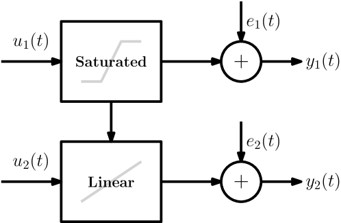
Figure 1: A block diagram of the system used in Example V-C.

Note that, for sufficiently low amplitudes $A$, $x_{1}(t)$ will be smaller than the saturation level $a=2$ for all $t$, and thus the system will behave as a linear system. However, when $A$ increases, the saturation will affect the system output more and more. The RMSE was computed for eight different amplitudes $A$, and the result is shown in Fig. 2. It can be seen that for small amplitudes, when the system is effectively linear, the Arx model gives a marginally better result than Lava-R and Wave. However, as the amplitude is increased, the nonlinear effects become more important, and Lava-R outperforms both Wave and Arx models.

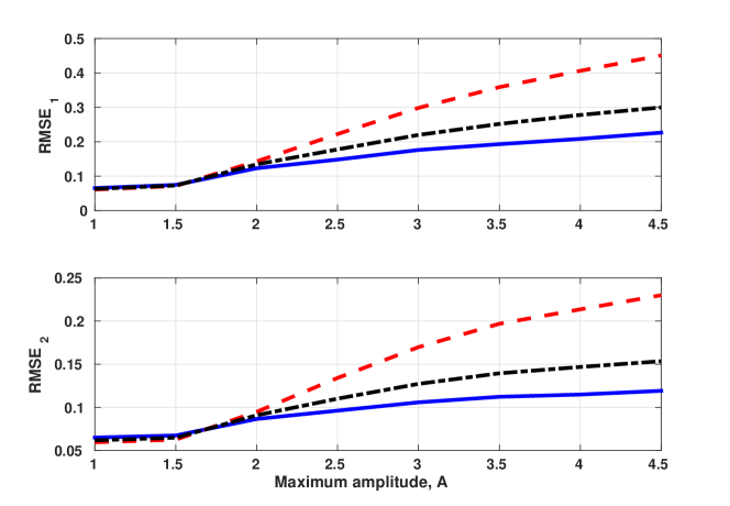
Figure 2: The RMSE for Example (V-C) computed for different input amplitudes, using Lava-R (solid), affine Arx (dashed) and Wave (dash-dotted).

V-D Water tank

In this example a real cascade tank process is studied. It consists of two tanks mounted on top of each other, with free outlets. The top tank is fed with water by a pump. The input signal is the voltage applied to the pump, and the output consists of the water level in the two tanks. The setup is described in more detail in [34]. The data set consists of 2500 samples collected every five seconds. The first 1250 samples where used for identification, and the last 1250 samples for validation.

Figure 3: The output in Example V-D (blue), plotted together with the output of the model identified by Lava-R (red). The system was identified using the first 1250 data samples. The validation set consisted of the remaining 1250 samples.

The identification was performed using $n_{a}=2$, $n_{b}=2$ and $M=3$. With two outputs, this results in 14 parameters in $\boldsymbol{\Theta}$ and 1458 parameters in $\mathbf{Z}$. Lava-R found a model with only 37 nonzero parameters in $\mathbf{Z}$, and the simulated output together with the measured output are shown in Fig. 3. The FIT values, computed on the validation data are shown in Table I. It can be seen that an affine ARX model gives a good fit, but also that using Lava-R the FIT measure can be improved significantly. In this example, Wave did not perform very well.

TABLE I: FIT for Example V-D.

	Lava-R	Wave	Arx
Upper tank	$91.6\%$	$79.2\%$	$84.9\%$
Lower tank	$90.8\%$	$76.9\%$	$78.6\%$

V-E Pick-and-place machine

In the final example, a real pick-and-place machine is studied. This machine is used to place electronic components on a circuit board, and is described in detail in [13]. This system exhibits saturation, different modes, and other nonlinearities. The data used here are from a real physical process, and were also used in e.g. [3, 14, 20]. The data set consists of a 15s recording of the single input $u(t)$ and the vertical position of the mounting head $y(t)$. The data was sampled at 50 Hz, and the first 8s ($N=400$) were used for identification and the last 7s for validation.

The identification was performed using $n_{a}=2$, $n_{b}=2$ and $M=6$. For the SISO system considered here, this results in 5 parameters in $\boldsymbol{\Theta}$ and 1296 parameters in $\mathbf{Z}$. Lava-R found a model with 33 of the parameters in $\mathbf{Z}$ being nonzero, the output of which is shown in Fig. 4.

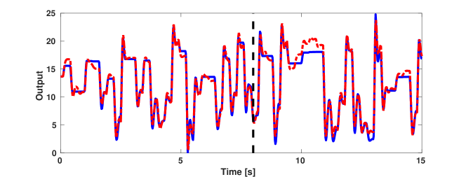
Figure 4: The output in Example V-E (blue), plotted together with the output of the model identified by Lava-R (red). The system was identified using the first part of the data, while the validation set consisted of the remaining samples indicated after the dashed line.

TABLE II: FIT for Example V-E.

	Lava-R	Wave	Arx
FIT	$83.2\%$	$78.2\%$	$73.1\%$

The FIT values, computed on the validation data, for Lava-R, Wave and affine Arx are shown in Table II. Lava-R outperforms Narx using wavelet networks, and both are better than Arx.

VI Conclusion

We have developed a method for learning nonlinear systems with multiple outputs and inputs. We began by modelling the errors of a nominal predictor using a latent variable formulation. The nominal predictor could for instance be a linear approximation of the system but could also include known nonlinearities. A learning criterion was derived based on the principle of maximum likelihood, which obviates the tuning of regularization parameters. The criterion is then minimized using a majorization-minimization approach. Specifically, we derived a convex user-parameter free formulation, which led to a computationally efficient recursive algorithm that can be applied to large datasets as well as online learning problems.

The method introduced in this paper learns parsimonious predictor models and captures nonlinear system dynamics. This was illustrated via synthetic as well as real data examples. As shown in these examples a recursive implementation of the proposed method was capable of outperforming a batch method using a Narx model with a wavelet network.

Appendix A Derivation of the distributions (8) and (14)

We start by computing $p(\mathbf{Y}|\boldsymbol{\Omega})$ given in (7). The function $p(\mathbf{Y}|\boldsymbol{\Omega},\mathbf{Z})$ can be found from (1)–(4) and the chain rule:

$$\begin{split}p(\mathbf{Y}|\boldsymbol{\Omega},\mathbf{Z})&=\prod_{t=1}^{N}p_{\boldsymbol{\varepsilon}}(\mathbf{y}(t)-\boldsymbol{\Theta}\boldsymbol{\varphi}(t)|\mathcal{D}_{t-1},\mathbf{Z}),\end{split}$$ (39)

where we have neglected initial conditions [27]. Since

$$\begin{split}&p_{\boldsymbol{\varepsilon}}(\mathbf{y}(t)-\boldsymbol{\Theta}\boldsymbol{\varphi}(t)|\mathcal{D}_{t-1},\mathbf{Z})\propto\\ &\exp\left(-\frac{1}{2}\|\mathbf{y}(t)-\boldsymbol{\Theta}\boldsymbol{\varphi}(t)-\mathbf{Z}\boldsymbol{\gamma}(t)\|_{\boldsymbol{\Sigma}^{-1}}^{2}\right),\end{split}$$

it follows that

$$\begin{split}&p(\mathbf{Y}|\boldsymbol{\Omega},\mathbf{Z})=\\ &\frac{1}{\sqrt{(2\pi)^{n_{y}N}|\boldsymbol{\Sigma}|^{N}}}\exp\left(-\frac{1}{2}\|\mathbf{Y}-\boldsymbol{\Theta}\boldsymbol{\Phi}-\mathbf{Z}\boldsymbol{\Gamma}\|_{\boldsymbol{\Sigma}^{-1}}^{2}\right).\end{split}$$ (40)

Using the vectorized variable in (9)-(10) we can see that

$$\operatorname{vec}(\boldsymbol{\Theta}\boldsymbol{\Phi})=\mathbf{F}\boldsymbol{\theta}\quad\text{and}\quad\operatorname{vec}(\mathbf{Z}\boldsymbol{\Gamma})=\mathbf{G}\mathbf{z}.$$

and thus,

$$\|\mathbf{Y}-\boldsymbol{\Theta}\boldsymbol{\Phi}-\mathbf{Z}\boldsymbol{\Gamma}\|_{\boldsymbol{\Sigma}^{-1}}^{2}=\|\mathbf{y}-\mathbf{F}\boldsymbol{\theta}-\mathbf{G}\mathbf{z}\|_{\mathbf{I}_{N}\otimes\boldsymbol{\Sigma}^{-1}}^{2}.$$

Next, we note that the following useful equality holds:

$$\|\mathbf{y}-\mathbf{F}\boldsymbol{\theta}-\mathbf{G}\mathbf{z}\|_{\mathbf{I}_{N}\otimes\boldsymbol{\Sigma}^{-1}}^{2}+\|\mathbf{z}\|_{\mathbf{D}^{-1}}^{2}=\\ \|\mathbf{y}-\mathbf{F}\boldsymbol{\theta}\|_{\mathbf{R}^{-1}}^{2}+\|\mathbf{z}-\boldsymbol{\zeta}\|_{\mathbf{\Sigma}_{z}^{-1}}^{2}$$ (41)

where $\mathbf{R}$ is given by (11), $\boldsymbol{\zeta}$ by (15), and $\mathbf{\Sigma}_{z}$ by (16). To see that the equality holds, expand the norms on both sides of (41) and apply the matrix inversion lemma.

The sought-after distribution $p(\mathbf{Y}|\boldsymbol{\Omega})$ is given by (7). By using (41) it follows that

$$p(\mathbf{Y}|\boldsymbol{\Omega},\mathbf{Z})p(\mathbf{Z})\propto\\ \exp(-\frac{1}{2}\|\mathbf{y}-\mathbf{F}\boldsymbol{\theta}\|_{\mathbf{R}^{-1}}^{2})\exp(-\frac{1}{2}\|\mathbf{z}-\boldsymbol{\zeta}\|_{\mathbf{\Sigma}_{z}^{-1}}^{2}).$$ (42)

with the normalization constant $((2\pi)^{n_{y}(N+q)}|\boldsymbol{\Sigma}|^{N}|\mathbf{D}|)^{-1/2}$. Noting that

$$\int\exp\left(-\frac{1}{2}\|\mathbf{z}-\boldsymbol{\zeta}\|_{\mathbf{\Sigma}_{z}^{-1}}^{2}\right)d\mathbf{Z}=\sqrt{(2\pi)^{n_{y}q}|\mathbf{\Sigma}_{z}|}$$

it can be seen that

$$p(\mathbf{Y}|\boldsymbol{\Omega})=\frac{1}{\sqrt{(2\pi)^{Nn_{y}}|\mathbf{R}|}}\exp\left(-\frac{1}{2}\|\mathbf{y}-\mathbf{F}\boldsymbol{\theta}\|_{\mathbf{R}^{-1}}^{2}\right),$$ (43)

which proves (8). To obtain an expression for $p(\mathbf{Z}|\boldsymbol{\Omega},\mathbf{Y})$ simply insert (42) and (43) into Bayes’ rule to get (14).

Appendix B Derivation of the majorizing tangent plane (22)

The first-order Taylor expansion of the log-determinant can be written as

$$\begin{split}\ln|\mathbf{R}|&\simeq\ln|\widetilde{\mathbf{R}}|+(\partial_{\boldsymbol{\sigma}}\ln|\mathbf{R}|)|_{\mathbf{R}=\widetilde{\mathbf{R}}}(\boldsymbol{\sigma}-\widetilde{\boldsymbol{\sigma}})\\ &\quad+(\partial_{\mathbf{d}}\ln|\mathbf{R}|_{\mathbf{R}=\widetilde{\mathbf{R}}})(\mathbf{d}-\tilde{\mathbf{d}})\end{split}$$

where $\boldsymbol{\sigma}$ is the vector of diagonal elements in $\boldsymbol{\Sigma}$ and $\mathbf{d}$ contains the diagonal elements in $\mathbf{D}$.

For the derivatives with respect to $\mathbf{d}$ we have

$$\frac{\partial}{\partial d_{i,j}}\ln|\mathbf{R}|=\operatorname{tr}\left(\mathbf{R}^{-1}\frac{\partial\mathbf{R}}{\partial d_{i,j}}\right)=\operatorname{tr}\left(\mathbf{G}^{\top}\mathbf{R}^{-1}\mathbf{G}\frac{\partial\mathbf{D}}{\partial{d_{i,j}}}\right).$$

Note that

$$\sum_{i=1}^{n_{y}}\sum_{j=1}^{q}d_{i,j}\frac{\partial\mathbf{D}}{\partial d_{i,j}}=\mathbf{D}$$

so Hence

$$\partial_{\mathbf{d}}\ln|\mathbf{R}|_{\mathbf{R}=\widetilde{\mathbf{R}}}(\mathbf{d}-\tilde{\mathbf{d}})=\operatorname{tr}\left(\mathbf{G}^{\top}\widetilde{\mathbf{R}}^{-1}\mathbf{G}(\mathbf{D}-\widetilde{\mathbf{D}})\right).$$

In the same way

$$\partial_{\boldsymbol{\sigma}}\ln|\mathbf{R}|_{\mathbf{R}=\widetilde{\mathbf{R}}}(\boldsymbol{\sigma}-\tilde{\boldsymbol{\sigma}})=\operatorname{tr}\left(\widetilde{\mathbf{R}}^{-1}(\mathbf{I}_{N}\otimes(\boldsymbol{\Sigma}-\widetilde{\boldsymbol{\Sigma}})\right).$$

Since $\ln|\mathbf{R}|$ is concave in $\boldsymbol{\sigma}$ and $\mathbf{d}$, it follows that

$$\ln|\mathbf{R}|\leq\widetilde{K}+\operatorname{tr}\left(\mathbf{G}^{\top}\widetilde{\mathbf{R}}^{-1}\mathbf{G}\mathbf{D}\right)+\operatorname{tr}\left(\widetilde{\mathbf{R}}^{-1}(\mathbf{I}_{N}\otimes\boldsymbol{\Sigma})\right)$$ (44)

where

$$\widetilde{K}=\ln|\widetilde{\mathbf{R}}|-\operatorname{tr}\left(\mathbf{G}^{\top}\widetilde{\mathbf{R}}^{-1}\mathbf{G}\widetilde{\mathbf{D}}\right)-\operatorname{tr}\left(\widetilde{\mathbf{R}}^{-1}(\mathbf{I}_{N}\otimes\widetilde{\boldsymbol{\Sigma}})\right).$$

Appendix C Proof of Theorem 2

It follows from (21) that

$$\mathbf{R}=\sum_{i=1}^{n_{y}}(\mathbf{R}_{i}\otimes\mathbf{E}_{i,i})$$

where $\mathbf{R}_{i}=\boldsymbol{\Gamma}^{\top}\mathbf{D}_{i}\boldsymbol{\Gamma}+\sigma_{i}\mathbf{I}_{N}$. Hence,

$$\mathbf{R}^{-1}=\sum_{i=1}^{n_{y}}\left(\mathbf{R}_{i}^{-1}\otimes\mathbf{E}_{i,i}\right).$$

Thus, we can rewrite (25) as (to within an additive constant):

$$V^{\prime}(\boldsymbol{\Omega}|\mathbf{Z},\widetilde{\boldsymbol{\Omega}})=\sum_{i=1}^{n_{y}}\Bigl{(}\frac{1}{\sigma_{i}}\|\bar{\mathbf{y}}_{i}\|_{2}^{2}+\|\mathbf{z}_{i}\|_{\mathbf{D}_{i}^{-1}}^{2}+\\ \sigma_{i}\operatorname{tr}(\widetilde{\mathbf{R}}_{i}^{-1})+\operatorname{tr}(\boldsymbol{\Gamma}\widetilde{\mathbf{R}}_{i}^{-1}\boldsymbol{\Gamma}^{\top}\mathbf{D}_{i})\Bigr{)}.$$ (45)

where $\bar{\mathbf{y}}_{i}=\mathbf{y}_{i}-\boldsymbol{\Phi}^{\top}\boldsymbol{\theta}_{i}-\boldsymbol{\Gamma}^{\top}\mathbf{z}_{i}$.

We next derive analytical expressions for the $\boldsymbol{\Sigma}$ and $\mathbf{D}$ that minimize $V^{\prime}(\boldsymbol{\Omega}|\mathbf{Z},\widetilde{\boldsymbol{\Omega}})$. Note that

$$\frac{\partial}{\partial\sigma_{i}}V^{\prime}(\boldsymbol{\Omega}|\mathbf{Z},\widetilde{\boldsymbol{\Omega}})=-\frac{1}{\sigma_{i}^{2}}\|\bar{\mathbf{y}}_{i}\|_{2}^{2}+\operatorname{tr}(\widetilde{\mathbf{R}}_{i}^{-1}),$$

and setting the derivative to zero yields the estimate (29). In the same way it can be seen that the minimum of $d_{i,j}$ is attained at (29).

Inserting $\hat{\sigma}_{i}$ and $\hat{d}_{i,j}$ into (45), we see that we can find the minimizing $\boldsymbol{\Theta}$ and $\mathbf{Z}$ by minimizing

$$2 \sum_{i=1}^{n_{y}}\Bigl{(}\sqrt{\operatorname{tr}(\widetilde{\mathbf{R}}_{i}^{-1})}\|\mathbf{y}_{i}-\boldsymbol{\Phi}^{\top}\boldsymbol{\theta}_{i}-\boldsymbol{\Gamma}^{\top}\mathbf{z}_{i}\|_{2}+$$

$$\sum_{j=1}^{q}|z_{i,j}|\sqrt{\overline{\boldsymbol{\gamma}}_{j}^{\top}\widetilde{\mathbf{R}}_{i}^{-1}\overline{\boldsymbol{\gamma}}_{j}}\Bigr{)}.$$

Since term $i$ in the above sum is invariant with respect to $\boldsymbol{\theta}_{k}$ and $\mathbf{z}_{k}$ for $k\neq i$, we can divide term $i$ by $2\sqrt{\operatorname{tr}(\widetilde{\mathbf{R}}_{i}^{-1})}$, and see that minimizing the criterion above is equivalent to (26).

Appendix D Proof of Theorem 3

Initializing (18) at $\overline{\boldsymbol{\Omega}}_{0}=\{\mathbf{0},\mathbf{0},\mathbf{I}_{n_{y}}\}$ and $\boldsymbol{\Omega}_{0}=\{\boldsymbol{\Theta}_{0},\mathbf{0},\boldsymbol{\Sigma}_{0}\}$ where $\boldsymbol{\Sigma}_{0}=\text{diag}(\sigma^{(0)}_{1},\ldots,\sigma^{(0)}_{n_{y}})$, produces two sequences denoted $\overline{\boldsymbol{\Omega}}_{k}=\{\overline{\boldsymbol{\Theta}}_{k},\overline{\mathbf{D}}_{k},\overline{\boldsymbol{\Sigma}}_{k}\}$ and $\boldsymbol{\Omega}_{k}=\{\boldsymbol{\Theta}_{k},\mathbf{D}_{k},\boldsymbol{\Sigma}_{k}\}$ for $k>0$, respectively. This results also in sequences $\overline{\mathbf{Z}}_{k}$ and $\mathbf{Z}_{k}$. The theorem states that:

$$\boldsymbol{\Theta}_{k}=\overline{\boldsymbol{\Theta}}_{k}\quad\text{and}\quad\mathbf{Z}_{k}=\overline{\mathbf{Z}}_{k}$$ (46)

$$\mathbf{D}_{k}-\overline{\mathbf{D}}_{k}\rightarrow\mathbf{0}\quad\text{and}\quad\boldsymbol{\Sigma}_{k}-\overline{\boldsymbol{\Sigma}}_{k}\rightarrow\mathbf{0}.$$ (47)

We now show the stronger result that the covariance matrices converge as

$$\mathbf{D}_{i}^{(k)}=c_{i}^{(k)}\overline{\mathbf{D}}_{i}^{(k)},\quad\sigma_{i}^{(k)}=c_{i}^{(k)}\overline{\sigma}_{i}^{(k)},\quad\forall k>0,$$ (48)

where $c_{i}^{(k)}=(\sigma^{(0)}_{i})^{\frac{1}{2^{k}}}$. Note that $c_{i}^{(k)}\rightarrow 1$ as $k\rightarrow\infty$. Hence (48) implies (47). We prove (48) and (46) by induction. That (48) and (46) holds for $k=1$ follows directly from Theorem 2. Now assume that (48) holds for some $k\geq 1$. Let

$$\overline{\mathbf{R}}_{i} =\boldsymbol{\Gamma}\overline{\mathbf{D}}_{i}^{(k)}\boldsymbol{\Gamma}^{\top}+\overline{\sigma}_{i}^{(k)}\mathbf{I}_{N},$$

$$\widetilde{\mathbf{R}}_{i} =\boldsymbol{\Gamma}\mathbf{D}_{i}^{(k)}\boldsymbol{\Gamma}^{\top}+\sigma_{i}^{(k)}\mathbf{I}_{N}=c_{i}^{(k)}\overline{\mathbf{R}}_{i},$$

where the last equality follows by the assumption in (48). Therefore the weights used to estimate $\boldsymbol{\Theta}_{k+1}$ and $\mathbf{Z}_{k+1}$ are the same as those used to estimate $\overline{\boldsymbol{\Theta}}_{k+1},\overline{\mathbf{Z}}_{k+1}$:

$$w_{i,j}=\sqrt{\frac{{\boldsymbol{\gamma}}_{j}^{\top}\widetilde{\mathbf{R}}_{i}^{-1}{\boldsymbol{\gamma}}_{j}}{\operatorname{tr}(\widetilde{\mathbf{R}}_{i}^{-1})}}=\sqrt{\frac{{\boldsymbol{\gamma}}_{j}^{\top}\overline{\mathbf{R}}_{i}^{-1}{\boldsymbol{\gamma}}_{j}}{\operatorname{tr}(\overline{\mathbf{R}}_{i}^{-1})}},$$

so we can conclude that $\boldsymbol{\Theta}_{k+1}=\overline{\boldsymbol{\Theta}}_{k+1}$ and $\mathbf{Z}_{k+1}=\overline{\mathbf{Z}}_{k+1}$. The estimate $\mathbf{D}_{k+1}$ is given by

$$d_{i,j}^{(k+1)}=\frac{|z_{i,j}|}{\sqrt{{\boldsymbol{\gamma}}_{j}^{\top}\widetilde{\mathbf{R}}_{i}^{-1}{\boldsymbol{\gamma}}_{j}}}=\frac{\sqrt{c_{i}^{(k)}}|z_{i,j}|}{\sqrt{{\boldsymbol{\gamma}}^{\top}\overline{\mathbf{R}}^{-1}{\boldsymbol{\gamma}}}}=c_{i}^{(k+1)}\overline{d}_{i,j}^{(k+1)}$$

so $\mathbf{D}_{i}^{(k+1)}=c_{i}^{(k+1)}\overline{\mathbf{D}}_{i}^{(k+1)}$, and in the same way it can be seen that $\sigma_{i}^{(k+1)}=c_{i}^{(k+1)}\overline{\sigma}_{i}^{(k+1)}$. Hence by induction (48) and (46) are true for all $k>0$ and Theorem 3 follows.

Appendix E Derivation of the proposed recursive algorithm

In order to minimize $V^{\prime}(\mathbf{Z})$ we use a cyclic algorithm. That is, we minimize with respect to one component at a time. We follow an approach similar to that in [36], with the main difference being that here we consider arbitrary nonnegative weights $\mathbf{w}_{i}$.

Note that minimization of $V^{\prime}(\mathbf{Z})$ with respect to $z_{i,j}$ is equivalent to minimizing

$$V^{\prime}(z_{i,j})=\|\tilde{\boldsymbol{\xi}}_{i,j}-\mathbf{c}_{j}z_{i,j}\|_{2}+w_{i,j}|z_{i,j}|$$

where

$$\tilde{\boldsymbol{\xi}}_{i,j}=\boldsymbol{\xi}_{i}-\sum_{k\neq j}\mathbf{c}_{k}z_{i,k},\quad\mathbf{c}_{j}=[\boldsymbol{\Gamma}^{\top}-\boldsymbol{\Phi}^{\top}\mathbf{H}]_{j}.$$

As in [36] it can be shown that the sign of the optimal $\hat{z}_{i,j}$ is given by $\text{sign}(\hat{z}_{i,j})=\text{sign}(\mathbf{c}_{j}^{\top}\tilde{\boldsymbol{\xi}}_{i,j}).$ Hence we only have to find the absolute value $r_{i,j}=|z_{i,j}|$. Let

$$\alpha_{i,j}=\|\tilde{\boldsymbol{\xi}}_{i,j}\|_{2}^{2},\quad\beta_{j}=\|\mathbf{c}_{j}\|_{2}^{2},\quad g_{i,j}=\mathbf{c}_{j}^{\top}\tilde{\boldsymbol{\xi}}_{i,j}.$$

It is then straightforward to verify that the minimization of $V^{\prime}(z_{i,j})$ is equivalent to minimizing

$$V^{\prime}(r_{i,j})=(\alpha_{i,j}+\beta_{j}r_{i,j}^{2}-2g_{i,j}r_{i,j})^{1/2}+w_{i,j}r_{i,j},$$

over all $r_{i,j}\geq 0$, and then setting $\hat{z}_{i,j}=\text{sign}(g_{i,j})\hat{r}_{i,j}$. From the Cauchy-Schwartz inequality it follows that

$$\alpha_{i,j}\beta_{i,j}\geq g_{i,j}^{2}.$$

Using this inequality it was shown in [36] that $V^{\prime}(r_{i,j})$ is a convex function. The derivative of $V^{\prime}(r_{i,j})$ is given by (dropping the subindices for now),

$$\frac{dV^{\prime}}{dr}=\frac{\beta r-|g|}{(\beta r^{2}-2|g|r+\alpha)^{1/2}}+w.$$ (49)

Since $V^{\prime}(r)$ is convex it follows that it is minimized by $r=0$ if and only if $dV^{\prime}(0)/dr\geq 0$, i.e., if and only if

$$\alpha w^{2}\geq g^{2}.$$ (50)

Next we study the case when $g^{2}>\alpha w^{2}$. It then follows from (49) that the stationary points of $V^{\prime}(r)$ satisfy

$$(\beta r-|g|)=-w(\beta r^{2}-2|g|r+\alpha)^{1/2}$$ (51)

Solving this equation for $r$ we get the stationary point

$$\hat{r}=\frac{|g|}{\beta}-\frac{w}{\beta\sqrt{\beta-w^{2}}}\sqrt{\alpha\beta-g^{2}}.$$

Hence we can conclude that the minimizer of $V^{\prime}(z_{i,j})$ is given by

$$\hat{z}_{i,j}=\left\{\begin{array}[]{ll}\text{sign}(g_{i,j})\hat{r}_{i,j}&\text{if }\alpha_{i,j}w_{i,j}^{2}<g_{i,j}^{2}\\ 0&\text{otherwise}\end{array}\right..$$

Next we show how to obtain this estimate using only recursively computed quantities. Let

$$\mathbf{T} =(\boldsymbol{\Gamma}^{\top}-\boldsymbol{\Phi}^{\top}\mathbf{H})^{\top}(\boldsymbol{\Gamma}^{\top}-\boldsymbol{\Phi}^{\top}\mathbf{H})$$ (52)

$$\kappa_{i} =\|\boldsymbol{\xi}_{i}\|_{2}^{2}$$ (53)

$$\rho_{i} =(\boldsymbol{\Gamma}^{\top}-\boldsymbol{\Phi}^{\top}\mathbf{H})^{\top}\boldsymbol{\xi}_{i}$$ (54)

$$\eta_{i} =\|\boldsymbol{\xi}_{i}-(\boldsymbol{\Gamma}^{\top}-\boldsymbol{\Phi}^{\top}\mathbf{H})\mathbf{z}_{i}\|_{2}^{2}$$ (55)

$$\zeta_{i} =(\boldsymbol{\Gamma}^{\top}-\boldsymbol{\Phi}^{\top}\mathbf{H})(\boldsymbol{\xi}_{i}-(\boldsymbol{\Gamma}^{\top}-\boldsymbol{\Phi}^{\top}\mathbf{H})\mathbf{z}_{i})$$ (56)

Then it is straightforward to show that

$$\alpha_{i,j} =\eta_{i}+\beta_{j}z_{i,j}^{2}+2\zeta_{i,j}z_{i,j}$$

$$\beta_{j} =\mathbf{T}_{j,j}$$

$$g_{i,j} =\zeta_{i,j}+\beta_{j}z_{i,j}.$$

Also define $\boldsymbol{\Psi}^{\mathbf{a},\mathbf{b}}(t)$ recursively, for any two vector-valued signals $\mathbf{a}(t)$, $\mathbf{b}(t)$, as

$$\boldsymbol{\Psi}^{\mathbf{a},\mathbf{b}}(0) =\mathbf{0}$$ (57)

$$\boldsymbol{\Psi}^{\mathbf{a},\mathbf{b}}(t+1) =\boldsymbol{\Psi}^{\mathbf{a},\mathbf{b}}(t)+\mathbf{a}(t)\mathbf{b}^{\top}(t).$$ (58)

Note that $\boldsymbol{\Psi}^{\mathbf{a},\mathbf{b}}(t)=(\boldsymbol{\Psi}^{\mathbf{b},\mathbf{a}}(t))^{\top}$. It can be verified that all quantities (52)–(56), and thus $\hat{z}_{i,j}$, can be coputed from $\boldsymbol{\Psi}^{\cdot,\cdot}(N)$.

The full algorithm for updating the needed quantities, including the update of $\overline{\boldsymbol{\Theta}}$ and $\mathbf{H}$, is summarized in Algorithm 1. Note that the iterations of the outer for-loop can be executed in parallel.

Algorithm 1 : Recursive solution to (26)

1:Input: $\mathbf{y}(t)$, $\boldsymbol{\varphi}(t)$, $\boldsymbol{\gamma}(t)$, $\check{\boldsymbol{\Theta}}$ and $\check{\mathbf{Z}}$

2:Update $\mathbf{P}(t)$, $\overline{\boldsymbol{\Theta}}(t)$ and $\mathbf{H}(t)$ according to (32)-(34).

3:Update $\boldsymbol{\Psi}^{\boldsymbol{\varphi},\boldsymbol{\varphi}}(t)$, $\boldsymbol{\Psi}^{\boldsymbol{\gamma},\boldsymbol{\gamma}}(t)$, $\boldsymbol{\Psi}^{\mathbf{y},\mathbf{y}}(t)$, $\boldsymbol{\Psi}^{\boldsymbol{\varphi},\boldsymbol{\gamma}}(t)$, $\boldsymbol{\Psi}^{\boldsymbol{\varphi},\mathbf{y}}(t)$ and $\boldsymbol{\Psi}^{\boldsymbol{\gamma},\mathbf{y}}(t)$ according to (58) .

4:$\mathbf{T}=\boldsymbol{\Psi}^{\boldsymbol{\gamma},\boldsymbol{\gamma}}-\boldsymbol{\Psi}^{\boldsymbol{\gamma},\boldsymbol{\varphi}}\mathbf{H}-\mathbf{H}^{\top}\boldsymbol{\Psi}^{\boldsymbol{\varphi},\boldsymbol{\gamma}}+\mathbf{H}^{\top}\boldsymbol{\Psi}^{\boldsymbol{\varphi},\boldsymbol{\varphi}}\mathbf{H}$.

5:for $i=1,\dots,n_{y}$ do

6:     $\kappa=\boldsymbol{\Psi}^{\mathbf{y},\mathbf{y}}_{i,i}+\tilde{\boldsymbol{\theta}}_{i}^{\top}\boldsymbol{\Psi}^{\boldsymbol{\varphi},\boldsymbol{\varphi}}\tilde{\boldsymbol{\theta}}_{i}-2\tilde{\boldsymbol{\theta}}_{i}^{\top}[\boldsymbol{\Psi}^{\boldsymbol{\varphi},\mathbf{y}}]_{i}$.

7:     $\rho=[\boldsymbol{\Psi}^{\boldsymbol{\gamma},\mathbf{y}}]_{i}-\boldsymbol{\Psi}^{\boldsymbol{\gamma},\boldsymbol{\varphi}}\tilde{\boldsymbol{\theta}}_{i}-\mathbf{H}^{\top}[\boldsymbol{\Psi}^{\boldsymbol{\varphi},\boldsymbol{\gamma}}]_{i}+\mathbf{H}^{\top}\boldsymbol{\Psi}^{\boldsymbol{\varphi},\boldsymbol{\varphi}}\tilde{\boldsymbol{\theta}}_{i}$.

8:     $\eta=\kappa-2\rho^{\top}\check{\mathbf{z}}_{i}+\check{\mathbf{z}}_{i}^{\top}\mathbf{T}\check{\mathbf{z}}_{i}$.

9:     $\zeta=\rho-\mathbf{T}\check{\mathbf{z}}_{i}$

10:     repeat

11:         for  $j=1,\dots,q$  do

12:              $\alpha=\eta+\mathbf{T}_{j,j}\check{z}_{i,j}^{2}+2\zeta_{j}\check{z}_{i,j}$.

13:              $g=\zeta_{j}+\mathbf{T}_{j,j}\check{z}_{i,j}$.

14:              $\beta=\mathbf{T}_{j,j}$.

15:              $\hat{r}=\frac{|g|}{\beta}-\frac{w_{i,j}}{\beta\sqrt{\beta-w_{i,j}^{2}}}\sqrt{\alpha\beta-g^{2}}$.

16:              $\hat{z}_{i,j}=\left\{\begin{array}[]{ll}\text{sign}(g)\hat{r}&\text{if }\alpha w_{i,j}^{2}<g^{2}\\ 0&\text{otherwise}\end{array}\right.$

17:              $\eta:=\eta+\mathbf{T}_{j,j}(\check{z}_{i,j}-\hat{z}_{i,j})+2(\check{z}_{i,j}-\hat{z}_{i,j})\zeta_{j}$.

18:              $\zeta:=\zeta+[\mathbf{T}]_{j}(\check{z}_{i,j}-\hat{z}_{i,j})$.

19:              $\check{z}_{i,j}:=\hat{z}_{i,j}$.

20:         end for

21:     until number of iterations equals $L$.

22:end for

23:$\widehat{\mathbf{Z}}=\check{\mathbf{Z}}$.

24:$\widehat{\boldsymbol{\Theta}}=\overline{\boldsymbol{\Theta}}-\widehat{\mathbf{Z}}\mathbf{H}$.

25:Output: $\widehat{\boldsymbol{\Theta}},\widehat{\mathbf{Z}}$.

References

• [1] E. W. Bai and Y. Liu. Recursive direct weight optimization in nonlinear system identification: A minimal probability approach. Automatic Control, IEEE Transactions on, 52(7):1218–1231, 2007.
• [2] D. Barber. Bayesian reasoning and machine learning. Cambridge University Press, 2012.
• [3] A. Bemporad, A. Garulli, S. Paoletti, and A. Vicino. A bounded-error approach to piecewise affine system identification. IEEE Trans. Automatic Control, 50(10):1567–1580, Oct 2005.
• [4] H. Bijl, J. W. van Wingerden, T. Schön, and M. Verhaegen. Online sparse gaussian process regression using fitc and pitc approximations. IFAC-PapersOnLine, 48(28):703–708, 2015.
• [5] S. Billings. Nonlinear System Identification: NARMAX Methods in the Time, Frequency, and Spatio-Temporal Domains. Wiley, 2013.
• [6] C. M. Bishop. Pattern Recognition and Machine Learning. Springer, 2006.
• [7] G. E. Box, G. M. Jenkins, G. C. Reinsel, and G. M. Ljung. Time Series Analysis: Forecasting and Control. John Wiley & Sons, 2015.
• [8] H. Chen. Extended recursive least squares algorithm for nonlinear stochastic systems. In American Control Conference, 2004. Proceedings of the 2004, volume 5, pages 4758–4763. IEEE, 2004.
• [9] A. P. Dempster, N. M. Laird, and D. B. Rubin. Maximum likelihood from incomplete data via the em algorithm. Journal of the royal statistical society. Series B (methodological), pages 1–38, 1977.
• [10] M. Enqvist. Linear models of nonlinear systems. PhD thesis, Linköping University, Linköping, Sweden, 2005.
• [11] F. Giri and E. W. Bai. Block-oriented nonlinear system identification, volume 1. Springer, 2010.
• [12] D. R. Hunter and K. Lange. A tutorial on MM algorithms. The American Statistician, 58(1):30–37, 2004.
• [13] A. Juloski, W. Heemels, and G. Ferrari-Trecate. Data-based hybrid modelling of the component placement process in pick-and-place machines. Control Engineering Practice, 12(10):1241–1252, 2004.
• [14] A. L. Juloski, S. Paoletti, and J. Roll. Recent techniques for the identification of piecewise affine and hybrid systems. In L. Menini, L. Zaccarian, and C. Abdallah, editors, Current Trends in Nonlinear Systems and Control, pages 79–99. Birkhäuser Boston, 2006.
• [15] L. Ljung. System Identification: Theory for the User. Pearson Education, 1998.
• [16] L. Ljung. Model validation and model error modeling. In The Åström Symposium on Control, pages 15–42. Studentlitteratur, 1999.
• [17] L. Ljung. System identification toolbox for use with MATLAB. The MathWorks, Inc., 2007.
• [18] L. Ljung and T. Söderström. Theory and Practice of Recursive Identification. MIT Press, Cambridge, MA, 1983.
• [19] P. Mattsson and T. Wigren. Convergence analysis for recursive Hammerstein identification. Automatica, 71:179–186, 2016.
• [20] H. Ohlsson and L. Ljung. Identification of switched linear regression models using sum-of-norms regularization. Automatica, 49(4):1045–1050, 2013.
• [21] J. Paduart, L. Lauwers, J. Swevers, K. Smolders, Johan Schoukens, and Rik Pintelon. Identification of nonlinear systems using polynomial nonlinear state space models. Automatica, 46(4):647 – 656, 2010.
• [22] G. Pillonetto. Consistent identification of wiener systems: A machine learning viewpoint. Automatica, 49(9):2704–2712, 2013.
• [23] G. Pillonetto, F. Dinuzzo, T. Chen, G. De Nicolao, and Lennart Ljung. Kernel methods in system identification, machine learning and function estimation: A survey. Automatica, 50(3):657–682, 2014.
• [24] J. Roll, A. Nazin, and L. Ljung. Nonlinear system identification via direct weight optimization. Automatica, 41(3):475–490, 2005.
• [25] J. Schoukens, M. Vaes, and R. Pintelon. Linear system identification in a nonlinear setting: Nonparametric analysis of the nonlinear distortions and their impact on the best linear approximation. IEEE Control Systems, 36(3):38–69, 2016.
• [26] J. Sjöberg, Q. Zhang, L. Ljung, A. Benveniste, Bernard Delyon, Pierre-Yves Glorennec, Håkan Hjalmarsson, and Anatoli Juditsky. Nonlinear black-box modeling in system identification: a unified overview. Automatica, 31(12):1691 – 1724, 1995.
• [27] T. Söderström and P. Stoica. System identification. Prentice-Hall, Inc., 1988.
• [28] A. Solin and S. Särkkä. Hilbert space methods for reduced-rank Gaussian process regression, 2014. arXiv preprint arXiv:1401.5508.
• [29] P. Stoica and P. Åhgren. Exact initialization of the recursive least-squares algorithm. International Journal of Adaptive Control and Signal Processing, 16(3):219–230, 2002.
• [30] P. Stoica, D. Zachariah, and J. Li. Weighted SPICE: A unifying approach for hyperparameter-free sparse estimation. Digital Signal Processing, 33:1–12, 2014.
• [31] S. Tayamon, T. Wigren, and J. Schoukens. Convergence analysis and experiments using an RPEM based on nonlinear ODEs and midpoint integration. In Decision and Control (CDC), 2012 IEEE 51st Annual Conference on, pages 2858–2865. IEEE, 2012.
• [32] P. Van den Hof and B. Ninness. System identification with generalized orthonormal basis functions. In Modelling and Identification with Rational Orthogonal Basis Functions, pages 61–102. Springer, 2005.
• [33] T. Wigren. Recursive prediction error identification using the nonlinear Wiener model. Automatica, 29(4):1011 – 1025, 1993.
• [34] T. Wigren. Recursive prediction error identification and scaling of non-linear state space models using a restricted black box parameterization. Automatica, 42(1):159 – 168, 2006.
• [35] T. T. Wu and K. Lange. The mm alternative to em. Statistical Science, 25(4):492–505, 2010.
• [36] D. Zachariah and P. Stoica. Online hyperparameter-free sparse estimation method. IEEE Trans. Signal Processing, 63(13):3348–3359, July 2015.