Solving Backward Stochastic Differential Equations
with quadratic-growth drivers
by Connecting the Short-term Expansions 

Abstract

This article proposes a new approximation scheme for quadratic-growth BSDEs in a Markovian setting by connecting a series of semi-analytic asymptotic expansions applied to short-time intervals. Although there remains a condition which needs to be checked a posteriori, one can avoid altogether time-consuming Monte Carlo simulation and other numerical integrations for estimating conditional expectations at each space-time node. Numerical examples of quadratic-growth as well as Lipschitz BSDEs suggest that the scheme works well even for large quadratic coefficients, and a fortiori for large Lipschitz constants.

Keywords : asymptotic expansion, discretization, quadratic-growth BSDEs

1 Introduction

The research on backward stochastic differential equations (BSDEs) was initiated by Bismut (1973) [8] for a linear case and followed by Pardoux & Peng (1990) [43] for general non-linear setups. Since then, BSDEs have attracted strong interests among researchers and now large amount of literature is available. See for example, El Karoui et al. (1997) [25], El Karoui & Mazliak (eds.) (1997) [24], Ma & Yong (2000) [39], Yong & Zhou (1999) [46], Cvitanić & Zhang (2013) [20] and Delong (2013) [21] for excellent reviews and various applications, and also Pardoux & Rascanu (2014) [44] for a recent thorough textbook for BSDEs in the diffusion setup. In particular, since the financial crisis in 2009, the importance of BSDEs in the financial industry has grown significantly. This is because BSDEs have been found to be indispensable to understand various valuation adjustments collectively referred to XVAs as well as the optimal risk control under the new regulations. For market developments and related issues, see Brigo, Morini & Pallavicini (2013) [14], Bianchetti & Morini (eds.) (2013) [7], Crépey & Bielecki (2014) [17] and references therein.

In the past decade, there has been also significant progress of numerical computation methods for BSDEs. In particular, based on the so-called $\mathbb{L}^{2}$-regularity of the control variables established by Zhang (2001, 2004) [52, 51], now standard backward Monte Carlo schemes for Lipschitz BSDEs have been developed by Bouchard & Touzi (2004) [11], Gobet, Lemor & Warin (2005) [32]. One can find many variants and extensions such as Bouchard & Elie (2008) [10] for BSDEs with jumps, Bouchard & Chassagneux (2008) [9] for reflected BSDEs, and Chassagneux & Richou (2016) [16] for a system of reflected BSDEs arising from optimal switching problems. Bender & Denk (2007) [4] proposed a forward scheme free from the linearly growing regression errors existing in the backward schemes; Bender & Steiner (2012) [5] suggested a possible improvement of the scheme [32] by using martingale basis functions for regressions; Crisan & Monolarakis (2014) [19] developed a second-order discretization using the cubature method. A different scheme based on the optimal quantization was proposed by Bally & Pagès (2003) [6]. See Pagès & Sagna (2017) [42] and references therein for its recent developments. Delarue & Menozzi (2006, 2008) [22, 23] studied a class of quasi-linear PDEs via a coupled forward-backward SDE with Lipschitz functions, which, in particular, becomes equivalent to a special type of quadratic-growth (qg) BSDE (so called deterministic KPZ equation) under a certain setting. Recently, Chassagneux & Richou (2016) [15] extended the standard backward scheme to qg-BSDEs with bounded terminal conditions in a Markovian setting.

As another approach, a semi-analytic approximation scheme was proposed by Fujii & Takahashi (2012) [27] and justified in the Lipschitz case by Takahashi & Yamada (2015) [48]. An efficient implementation algorithm based on an interacting particle method by Fujii & Takahashi (2015) [29] has been successfully applied to a large scale credit portfolio by Crépey & Song (2016) [18]. This is an asymptotic expansion around a linear driver motivated by the observation that, for many financial applications, the non-linear part of the driver is proportional to an interest rate spread and/or a default intensity which is, at most, of the order of a few percentage points. Although it cuts the cost of numerical computation drastically under many interesting situations, the non-linear effects may grow and cease to be perturbative when one deals with longer maturities, higher volatilities, or general risk-sensitive control problems for highly concave utility functions.

In this paper, we propose a new approximation scheme for Markovian qg-BSDEs with bounded terminal functions. The qg-BSDEs have many applications, in particular, they appear in exponential and power utility optimizations as well as mean-variance hedging problem. They are also relevant for a class of recursive utilities introduced by Epstein & Zin (1989) [26], which are widely used in economic theory. In addition, a successful scheme for qg-BSDEs possibly provides an unified computation method for a wide range of applications, since it is expected to be applicable also to the standard Lipschitz BSDEs. We try to achieve the advantages of both the standard Monte Carlo scheme, in terms of generality, and also the semi-analytic approximation scheme, in terms of the lesser numerical cost. The main idea is to decompose the original qg-BSDE into a sequence of qg-BSDEs each of which is defined in a short-time interval. We then employ an asymptotic expansion method to solve each of them approximately. In order to obtain the total error estimate, we first investigate the propagation of error for a sequence of qg-BSDEs with terminal conditions perturbed by bounded functions, say $\{\delta^{i}\}_{1\leq i\leq n}$. The first main result is thus obtained as Theorem 3.1. We then substitute the error function associated to the asymptotic expansion in each period for the function $\delta^{i}$, which then leads to our second main result of Theorem 4.1 providing the total error estimate for the proposed scheme.

Although there remains assumptions which cannot be confirmed a priori, which is a drawback of the current scheme, they can still be checked for each model a posteriori by numerical calculation. Once it is confirmed, the convergence with the rate of $n^{-1/2}$ in the strong sense is obtained for a finite range of discretization. In the case of the standard scheme with Monte Carlo simulation, although the convergence is guaranteed a priori for sufficiently small discretization and many paths, it is not completely free from a posteriori checks, either. One still needs to run heavy tests with varying discretization sizes and number of paths to confirm whether a given result provides a reasonable approximation or not. The advantage of the proposed scheme is that one can avoid time-consuming simulation for estimating conditional expectations at each space-time node by using simple semi-analytic results and thus finer discretization becomes easier to implement. We give numerical examples for both qg- and Lipschitz BSDEs to illustrate the empirical performance. They suggest that the scheme works well even for very large quadratic coefficients, and all the more so for large Lipschitz constants. Note also that, the short-term asymptotic expansion of qg-BSDEs in the strong sense is provided for the first time, which may be useful for other applications.

The organization of the paper is as follows: Section 2 explains the general setting and notations, Section 3 gives the time-discretization and investigates a sequence of qg-BSDEs perturbed in the terminal values; Section 4 applies the short-term expansion to the result of Section 3 which yields the total error estimate of the proposed scheme. Section 5 explains a concrete implementation using a discretized space-time grid and the corresponding error estimates. Section 6 provides numerical examples and also explain the relevant modifications when the scheme is applied to the Lipschitz BSDEs. We finally concludes in Section 7. Appendix A summarizes the properties of BMO-martingales, Appendices B and C derive the formula of the short-term asymptotic expansion and obtain the error estimates relevant for the analysis in the main text.

2 Preliminaries

2.1 General setting and notations

Throughout the paper, we fix the terminal time $T>0$. We work on the filtered probability space $(\Omega,{\cal F},\mathbb{F},\mathbb{P})$ carrying a $d$-dimensional independent standard Brownian motion $W$. $\mathbb{F}=({\cal F}_{t})_{t\in[0,T]}$ is the Brownian filtration satisfying the usual conditions augmented by the $\mathbb{P}$-null sets. We denote a generic positive constant by $C$, which may change line by line and it is sometimes associated with several subscripts (such as $C_{p,K}$) when there is a need to emphasize its dependency on those parameters. ${\cal T}^{T}_{0}$ denotes the set of all $\mathbb{F}$-stopping times $\tau:\Omega\rightarrow[0,T]$. We denote the sup-norm of $\mathbb{R}^{k}$-valued function $x:[0,T]\rightarrow\mathbb{R}^{k}$, $k\in\mathbb{N}$ by the symbol $||x||_{[a,b]}:=\sup\bigl{\{}|x_{t}|,t\in[a,b]\bigr{\}}$ and write $||x||_{t}:=||x||_{[0,t]}$.

Let us introduce the following spaces for stochastic processes with $p\geq 2$ and $k\in\mathbb{N}$. For the convenience of the reader, we separately summarize the relevant properties of the BMO martingales and the associated function spaces in Appendix A.
$\bullet~{}$${\cal S}^{p}_{[s,t]}(\mathbb{R}^{k})$ is the set of $\mathbb{R}^{k}$-valued adapted processes $X$ satisfying

$||X||_{{\cal S}^{p}_{[s,t]}}:=\mathbb{E}\bigl{[}||X||_{[s,t]}^{p}\bigr{]}^{1/p}<\infty~{}$.

$\bullet~{}$${\cal S}^{\infty}_{[s,t]}(\mathbb{R}^{k})$ is the set of $\mathbb{R}^{k}$-valued essentially bounded adapted processes $X$ satisfying

$||X||_{{\cal S}^{\infty}_{[s,t]}}:=\bigl{|}\bigl{|}\sup_{r\in[s,t]}|X_{r}|\bigr{|}\bigr{|}_{\infty}<\infty~{}$.

$\bullet~{}$${\cal H}^{p}_{[s,t]}(\mathbb{R}^{k})$ is the set of $\mathbb{R}^{k}$-valued progressively measurable processes $Z$ satisfying

$$||Z||_{{\cal H}^{p}_{[s,t]}}:=\mathbb{E}\Bigl{[}\Bigl{(}\int_{s}^{t}|Z_{r}|^{2}dr\Bigr{)}^{\frac{p}{2}}\Bigr{]}^{\frac{1}{p}}<\infty.$$

$\bullet~{}$${\cal K}^{p}{[s,t]}$ is the set of functions $(Y,Z)$ in the space ${\cal S}^{p}_{[s,t]}(\mathbb{R})\times{\cal H}^{p}_{[s,t]}(\mathbb{R}^{1\times d})$ with the norm defined by

$$||(Y,Z)||_{{\cal K}^{p}[s,t]}:=\bigl{(}||Y||^{p}_{{\cal S}^{p}_{[s,t]}}+||Z||^{p}_{{\cal H}^{p}_{[s,t]}}\bigr{)}^{1/p}~{}.$$

$\bullet~{}$$\mathbb{L}^{\infty}(\mathbb{R}^{d};\mathbb{R}^{k})$ is the set of measurable bounded functions $f:\mathbb{R}^{d}\rightarrow\mathbb{R}^{k}$.
$\bullet~{}$$C^{m}(\mathbb{R}^{d};\mathbb{R}^{k})$ is the set of $m$-time continuously differentiable functions $f:\mathbb{R}^{d}\rightarrow\mathbb{R}^{k}$.
$\bullet~{}$$C^{m}_{b}(\mathbb{R}^{d};\mathbb{R}^{k})$ is the subset of $C^{m}(\mathbb{R}^{d};\mathbb{R}^{k})$ with bounded derivatives.
$\bullet~{}$$C^{\infty}_{b}(\mathbb{R}^{d};\mathbb{R}^{k}):=\bigcap_{m\geq 1}C^{m}_{b}(\mathbb{R}^{d};\mathbb{R}^{k})$.

We frequently omit the arguments such as $\mathbb{R}^{d},~{}\mathbb{R}^{k}$ and subscript $[s,t]$ if they are obvious from the context. We use $\bigl{(}\Theta_{s},s\in[0,T]\bigr{)}$ as a collective argument $\Theta_{s}:=(Y_{s},Z_{s})$ to lighten the notation. We use the following notation for partial derivatives with respect to $x\in\mathbb{R}^{d}$ such that

$$\partial_{x}:=(\partial_{x^{1}},\cdots,\partial_{x^{d}}):=\bigl{(}\frac{\partial}{\partial x^{1}},\cdots,\frac{\partial}{\partial x^{d}}\bigr{)}$$

and $\partial_{\theta}:=(\partial_{y},\partial_{z})$ for the collective argument $\Theta$. We sometimes use the abbreviation $Z*W:=\int_{0}^{\cdot}Z_{s}dW_{s}$.

2.2 Setup

Firstly, we introduce the underlying forward process $X_{t},t\in[0,T]$:

$$X_{t}=x_{0}+\int_{0}^{t}b(r,X_{r})dr+\int_{0}^{t}\sigma(r,X_{r})dW_{r}~{},$$ (2.1)

where $x_{0}\in\mathbb{R}^{d}$ and $b:[0,T]\times\mathbb{R}^{d}\rightarrow\mathbb{R}^{d}$, $\sigma:[0,T]\times\mathbb{R}^{d}\rightarrow\mathbb{R}^{d\times d}$ are measurable functions.

Assumption 2.1.

(i) For all $t,t^{\prime}\in[0,T]$ and $x,x^{\prime}\in\mathbb{R}^{d}$, there exists a positive constant $K$ such that $~{}|b(t,x)-b(t^{\prime},x^{\prime})|+|\sigma(t,x)-\sigma(t^{\prime},x^{\prime})|\leq K\bigl{(}|t-t^{\prime}|^{\frac{1}{2}}+|x-x^{\prime}|\bigr{)}$.
(ii) $||b(\cdot,0)||_{T}+||\sigma(\cdot,0)||_{T}\leq K$.
(iii) $b$ and $\sigma$ are 3-time continuously differentiable with respect to $x$ and satisfy

$$|\partial_{x}^{m}b(t,x)|+|\partial_{x}^{m}\sigma(t,x)|\leq K~{},$$

$$|\partial_{x}^{m}b(t,x)-\partial_{x}^{m}b(t^{\prime},x)|+|\partial_{x}^{m}\sigma(t,x)-\partial_{x}^{m}\sigma(t^{\prime},x)|\leq K|t-t^{\prime}|^{1/2}~{},$$ (2.2)

for all $1\leq m\leq 3$, $t,t^{\prime}\in[0,T]$ and $x\in\mathbb{R}^{d}$.

Let us now introduce a qg-BSDE which is a target of our investigation:

$$Y_{t}=\xi(X_{T})+\int_{t}^{T}f(r,X_{r},Y_{r},Z_{r})dr-\int_{t}^{T}Z_{r}dW_{r},\quad t\in[0,T]$$ (2.3)

where $\xi:\mathbb{R}^{d}\rightarrow\mathbb{R}$, $f:[0,T]\times\mathbb{R}^{d}\times\mathbb{R}\times\mathbb{R}^{1\times d}\rightarrow\mathbb{R}$ are measurable functions.

Assumption 2.2.

(i) $f$ satisfies the quadratic structure condition [2]:

$$|f(t,x,y,z)|\leq l_{t}+\beta|y|+\frac{\gamma}{2}|z|^{2}$$

for all $(t,x,y,z)\in[0,T]\times\mathbb{R}^{d}\times\mathbb{R}\times\mathbb{R}^{1\times d}$, where $\beta\geq 0,\gamma>0$ are constants, $l:[0,T]\rightarrow\mathbb{R}_{+}$ is a positive function bounded by a constant $K$, i.e. $||l||_{T}\leq K$.
(ii) $f$ satisfies the continuity conditions such that, for all $t,t^{\prime}\in[0,T]$, $y,y^{\prime}\in\mathbb{R}$, $x,x^{\prime}\in\mathbb{R}^{d}$, $z,z^{\prime}\in\mathbb{R}^{1\times d}$,

$$|f(t,x,y,z)-f(t^{\prime},x,y,z)| \leq K|t-t^{\prime}|^{1/2}~{},$$

$$|f(t,x,y,z)-f(t,x,y^{\prime},z)| \leq K|y-y^{\prime}|~{},$$

$$|f(t,x,y,z)-f(t,x,y,z^{\prime})| \leq K\bigl{(}1+|z|+|z^{\prime}|\bigr{)}|z-z^{\prime}|~{},$$

$$|f(t,x,y,z)-f(t,x^{\prime},y,z)| \leq K\bigl{(}1+|y|+|z|^{2}\bigr{)}|x-x^{\prime}|.$$

(iii) the driver $f$ is 1-time continuously differentiable with respect to the spatial variables with continuous derivatives. In particular, we assume that

$$|\partial_{y}f(t,x,y,z)|\leq K,~{}\quad|\partial_{z}f(t,x,y,z)|\leq K(1+|z|),\quad|\partial_{x}f(t,x,y,z)|\leq K(1+|y|+|z|^{2})$$

for all $(t,x,y,z)\in[0,T]\times\mathbb{R}^{d}\times\mathbb{R}\times\mathbb{R}^{1\times d}$.
(iv) $\xi$ is a 3-time continuously differentiable function satisfying $||\xi(\cdot)||_{\mathbb{L}^{\infty}}\leq K$ and $||\partial_{x}^{m}\xi(\cdot)||_{\mathbb{L}^{\infty}}\leq K$ for every $1\leq m\leq 3$.

Remark 2.1.

The 2nd- and 3rd-order differentiability in Assumptions 2.1 and 2.2 is relevant only for the later part of the discussions (Section 4$\sim$), where the error estimate of the short-term expansions are required.

It has been well-known since the work of Kobylanski (2000) [36] that there exists a unique solution $(Y,Z)$ to (2.3) in the space $(Y,Z)\in{\cal S}^{\infty}\times{\cal H}^{2}_{BMO}$.

Lemma 2.1.

(universal bound) Under Assumptions 2.1 and 2.2, the solution $(Y,Z)\in{\cal S}^{\infty}\times{\cal H}^{2}_{BMO}$ of (2.3) satisfies

$$||Y||_{{\cal S}^{\infty}}\leq e^{\beta T}\Bigl{(}||\xi(\cdot)||_{\mathbb{L}^{\infty}}+T||l||_{T}\Bigr{)}~{},$$

$$||Z||_{{\cal H}^{2}_{BMO}}^{2}\leq\frac{e^{4\gamma||Y||_{{\cal S}^{\infty}}}}{\gamma^{2}}\Bigl{(}3+6\gamma T(\beta||Y||_{{\cal S}^{\infty}}+||l||_{T})\Bigr{)}~{}.$$

Proof.

This follows straightforwardly from the quadratic structure condition [2] which is given by Assumption 2.2 (i). See, for example, Lemma 3.1 and 3.2 in [30]. ∎

3 A sequence of qg-BSDEs perturbed in terminals

In this section, we investigate a sequence of qg-BSDEs. For each connecting point, we introduce a bounded measurable function $\delta^{i}:\mathbb{R}^{d}\rightarrow\mathbb{R}$ as perturbation. We then investigate the propagation of its effects to the total error.

3.1 Setup

Let us introduce a time partition $\pi:0=t_{0}<t_{1}<\cdots<t_{n}=T$. We put $h_{i}:=t_{i}-t_{i-1}$, $|\pi|:=\max_{1\leq i\leq n}h_{i}$. We denote each interval by $I_{i}:=[t_{i-1},t_{i}]$, $i\in\{1,\cdots,n\}$ and assume that there exists some positive constant $C$ such that $|\pi|n\leq C$ as well as $|\pi|/h_{i}\leq C$ for every $i\in\{1,\cdots,n\}$. In order to approximate the BSDE (2.3), we introduce a sequence of qg-BSDEs perturbed in the terminal values for each interval $t\in I_{i}$, $i\in\{1,\cdots,n\}$ in the following way:

$$\overline{Y}^{i}_{t}=\widehat{u}^{i+1}(X_{t_{i}})+\int_{t}^{t_{i}}f(r,X_{r},\overline{Y}^{i}_{r},\overline{Z}_{r}^{i})dr-\int_{t}^{t_{i}}\overline{Z}_{r}^{i}dW_{r}~{},$$ (3.1)

where $\widehat{u}^{i+1}:\mathbb{R}^{d}\rightarrow\mathbb{R}$ with $\widehat{u}^{n+1}(x):=\xi(x)$.

Each terminal function $\widehat{u}^{i+1}(x)$, $x\in\mathbb{R}^{d}$ of the period $I_{i}$ is defined by $\bigl{(}\overline{Y}^{i+1,t_{i},x}_{t},t\in[t_{i},t_{i+1}]\bigr{)}$, which is the solution of (3.1) for the period $I_{i+1}$ corresponding to the underlying process $X$ with the initial data $(t_{i},X_{t_{i}}=x)$ , and the additional perturbation term $\delta^{i+1}$

$$\widehat{u}^{i+1}(x) := \overline{Y}^{i+1,t_{i},x}_{t_{i}}-\delta^{i+1}(x),\quad i\in\{1,\cdots,n-1\}.$$ (3.2)

In the next section, $\{\delta^{i}\}_{i\leq n}$ will be related to the errors from the short-term expansion.

Assumption 3.1.

(i)The perturbation terms $\delta^{i+1}:\mathbb{R}^{d}\rightarrow\mathbb{R}$, $i\in\{1,\cdots,n\}$ are absolutely bounded measurable functions that keep $(\widehat{u}^{i+1})_{1\leq i\leq n}$ satisfying the conditions

$$(a) \max_{1\leq i\leq n}||\widehat{u}^{i+1}(\cdot)||_{\mathbb{L}^{\infty}}\leq K^{\prime},$$

$$(b) \max_{1\leq i\leq n}||\partial_{x}\widehat{u}^{i+1}(\cdot)||_{\mathbb{L}^{\infty}}\leq K^{\prime},$$

$$(c) \max_{1\leq i\leq n}||\partial_{x}^{m}\widehat{u}^{i+1}(\cdot)||_{\mathbb{L}^{\infty}}\leq K^{\prime},~{}(m\in\{2,3\})$$

with some $n$-independent positive constant $K^{\prime}$.
(ii) There exists an $n$-independent positive constant $C$ such that $\sum_{i=1}^{n-1}||\delta^{i+1}(\cdot)||_{\mathbb{L}^{\infty}}\leq C$.

We use the convention $\delta^{n+1}\equiv 0$ and $\overline{Y}^{n+1}_{t_{n}}=\xi(X_{t_{n}})$ in the following.

Remark 3.1.

The condition (i)(c) becomes relevant only for the short-term expansion in the next section.

Remark 3.2.

The classical (as well as variational) differentiability of qg-BSDEs is well-known by the works of Ankirchner et al. (2007) [1], Briand & Confortola (2008) [13] and Imkeller & Reis (2010) [33]. See Fujii & Takahashi (2017) [30] for the extension of these results to qg-BSDEs with Poisson random measures.

3.2 Properties of the solution

Applying the known results of qg-BSDE for each period, one sees that there exists a unique solution $(\overline{Y}^{i},\overline{Z}^{i})\in{\cal S}^{\infty}_{[t_{i-1},t_{i}]}\times{\cal H}^{2}_{BMO[t_{i-1},t_{i}]}$. Applying Lemma 2.1 for each period $I_{i}$, one also sees

$$||\overline{Y}^{i}||_{{\cal S}^{\infty}[t_{i-1},t_{i}]}\leq||\overline{Y}||_{{\cal S}^{\infty}}:=e^{\beta|\pi|}\Bigl{(}K^{\prime}+|\pi|||l||_{T}\Bigr{)}~{},$$ (3.3)

which is bounded uniformly in $i\in\{1,\cdots,n\}$, and so is $||\overline{Z}^{i}||_{{\cal H}^{2}_{BMO}[t_{i-1},t_{i}]}$.

Proposition 3.1.

Under Assumptions 2.1, 2.2 and Assumption 3.1 [i(a,b)], there exists some positive $(i,n)$-independent constant $C$ such that the process $\overline{Z}^{i}_{t},t\in I_{i}$ of the solution to the BSDE (3.1) satisfies

$$|\overline{Z}^{i}_{t}|\leq C(1+|X_{t}|),~{}t\in I_{i},~{}\text{$\mathbb{P}$-a.s.}$$

uniformly in $i\in\{1,\cdots,n\}$.

Proof.

We use the representation theorem for the control variable (Theorem 8.5 in [1]) and follow the arguments of Theorem 3.1 in Ma & Zhang (2002) [40]. Let us introduce the parameterized solution $(X^{t,x},\overline{Y}^{i,t,x},\overline{Z}^{i,t,x})$ with the initial data $(t,x)\in[t_{i-1},t_{i}]\times\mathbb{R}^{d}$:

$$X_{s}^{t,x}=x+\int_{t}^{s}b(r,X_{r}^{t,x})dr+\int_{t}^{s}\sigma(r,X_{r}^{t,x})dW_{r},$$ (3.4)

$$\overline{Y}^{i,t,x}_{s}=\widehat{u}^{i+1}(X_{t_{i}}^{t,x})+\int_{s}^{t_{i}}f(r,X_{r}^{t,x},\overline{Y}^{i,t,x}_{r},\overline{Z}_{r}^{i,t,x})dr-\int_{s}^{t_{i}}\overline{Z}_{r}^{i,t,x}dW_{r},$$ (3.5)

$s\in[t,t_{i}]$ where the classical differentiability of (3.4) and (3.5) with respect to the position $x$ is known [1]. The differential processes $(\partial_{x}X^{t,x},\partial_{x}\overline{Y}^{i,t,x},\partial_{x}\overline{Z}^{i,t,x})$ are given by the solutions to the following forward- and backward-SDE:

$$\partial_{x}X_{s}^{t,x}=\mathbb{I}+\int_{t}^{s}\partial_{x}b(r,X_{r}^{t,x})\partial_{x}X_{r}^{t,x}dr+\int_{t}^{s}\partial_{x}\sigma(r,X_{r}^{t,x})\partial_{x}X_{r}^{t,x}dW_{r},$$

$$\partial_{x}\overline{Y}_{s}^{i,t,x}=\partial_{x}\widehat{u}^{i+1}(X_{t_{i}}^{t,x})\partial_{x}X_{t_{i}}^{t,x}+\int_{t}^{t_{i}}\Bigl{\{}\partial_{x}f(r,X_{r}^{t,x},\overline{\Theta}^{i,t,x}_{r})\partial_{x}X_{r}^{t,x}$$

$$\qquad+\partial_{\theta}f(r,X_{r}^{t,x},\overline{\Theta}_{r}^{i,t,x})\partial_{x}\overline{\Theta}^{i,t,x}_{r}\Bigr{\}}dr-\int_{t}^{t_{i}}\partial_{x}\overline{Z}_{r}^{i,t,x}dW_{r},$$ (3.6)

where $\mathbb{I}$ is the $d\times d$ identity matrix and $\partial_{x}\overline{\Theta}^{i,t,x}=(\partial_{x}\overline{Y}^{i,t,x},\partial_{x}\overline{Z}^{i,t,x})$. Note that $|\partial_{y}f|$ is bounded and $|\partial_{z}f(r,X_{r}^{t,x},\overline{\Theta}_{r}^{i,t,x})|\leq K\bigl{(}1+|\overline{Z}_{r}^{i,t,x}|\bigr{)}$ by Assumption 2.2 (iii). By the facts given in (3.3) and the remark that follows, one sees $||\partial_{z}f(\cdot,X^{t,x}_{\cdot},\overline{\Theta}^{i,t,x}_{\cdot})||_{{\cal H}^{2}_{BMO[t,t_{i}]}}\leq C$ with some constant $C$. Thus Corollary 9 in [13] or Theorem A.1 in [30] implies that the BSDE (3.6) has a unique solution satisfying, for any $p\geq 2$,

$$\bigl{|}\bigl{|}\partial_{x}\overline{\Theta}^{i,t,x}\bigr{|}\bigr{|}^{p}_{{\cal K}^{p}[t,t_{i}]}\leq C_{p,{\bar{q}}}\mathbb{E}\Bigl{[}|\partial_{x}\widehat{u}^{i+1}(X_{t_{i}}^{t,x})\partial_{x}X_{t_{i}}^{t,x}|^{p{\bar{q}}^{2}}+\Bigl{(}\int_{t}^{t_{i}}|\partial_{x}f(r,X_{r}^{i,t,x},\overline{\Theta}_{r}^{i,t,x})\partial_{x}X_{r}^{i,t,x}|dr\Bigr{)}^{p{\bar{q}}^{2}}\Bigr{]}^{\frac{1}{{\bar{q}}^{2}}}$$

$$\quad\leq C_{p,{\bar{q}}}\mathbb{E}\Bigl{[}||\partial_{x}X^{t,x}||^{2p{\bar{q}}^{2}}_{[t,t_{i}]}\Bigr{]}^{\frac{1}{2{\bar{q}}^{2}}}\Bigl{(}1+h_{i}^{p}\mathbb{E}\Bigl{[}||\overline{Y}^{i}||_{[t,t_{i}]}^{2p{\bar{q}}^{2}}\Bigr{]}^{\frac{1}{2{\bar{q}}^{2}}}+\mathbb{E}\Bigl{[}\Bigl{(}\int_{t}^{t_{i}}|\overline{Z}_{r}^{i,t,x}|^{2}dr\Bigr{)}^{2p{\bar{q}}^{2}}\Bigr{]}^{\frac{1}{2{\bar{q}}^{2}}}\Bigr{)}$$ (3.7)

where ${\bar{q}}$ is a positive constant satisfying $q_{*}\leq{\bar{q}}<\infty$. Here, $q_{*}=\frac{r^{*}}{r^{*}-1}>1$ is the conjugate exponent of $r^{*}$ the upper bound of power with which the Reverse Hölder inequality holds for ${\cal E}(\partial_{z}f*W)$. We have used Assumption 2.2 (iv) and Hölder inequality in the last line.

By the standard estimate of SDE , one can show that $||\partial_{x}X^{t,x}||_{{\cal S}^{2p{\bar{q}}^{2}}}\leq C$ with some positive constant $C$ that is independent of the initial data $(t,x)$. The boundedness of $\overline{Y}^{i}$ in (3.3) and the following remark on $\overline{Z}^{i}$ together with Lemma A.1 show that the right-hand side of (3.7) is bounded by some positive constant. In particular, one can choose a common constant $C$ for every $i\in\{1,\cdots,n\}$ such that $|\partial_{x}\overline{Y}^{i,t,x}_{t}|\leq||\partial_{x}\overline{Y}^{i,t,x}||_{{\cal S}^{p}[t,t_{i}]}\leq C$ uniformly in $(t,x)\in[t_{i-1},t_{i}]\times\mathbb{R}^{d}$. By the representation theorem [1, 40], we have $\overline{Z}_{t}^{i}=\partial_{x}\overline{u}^{i}(t,X_{t})\sigma(t,X_{t}),~{}\forall t\in[t_{i-1},t_{i}]$, $\mathbb{P}$-a.s. where the function $\partial_{x}\overline{u}^{i}:[t_{i-1},t_{i}]\times\mathbb{R}^{d}\rightarrow\mathbb{R}^{1\times d}$ is defined by $\partial_{x}\overline{u}^{i}(t,x):=\partial_{x}\overline{Y}^{i,t,x}_{t}$. Now the Lipschitz property of $\sigma$ gives the desired result. ∎

Let us now define a progressively measurable process $\bigl{(}\overline{Z}_{t},t\in[0,T]\bigr{)}$ by

$$\overline{Z}_{t}:=\sum_{i=1}^{n}\overline{Z}_{t}^{i}\mathbb{1}_{\{t_{i-1}\leq t<t_{i}\}},~{}t\in[0,T]~{}$$ (3.8)

so that $\int_{0}^{T}|\overline{Z}_{t}|^{2}dt=\sum_{i=1}^{n}\int_{t_{i-1}}^{t_{i}}|\overline{Z}_{t}^{i}|^{2}dt$.

Proposition 3.2.

Under Assumptions 2.1, 2.2 and 3.1 [i(a), ii], the process $\bigl{(}\overline{Z}_{t},~{}t\in[0,T]\bigr{)}$ defined by (3.8) belongs to ${\cal H}^{2}_{BMO[0,T]}$ satisfying $||\overline{Z}||_{{\cal H}^{2}_{BMO}[0,T]}\leq C$ with some $n$-independent positive constant $C$.

Proof.

Applying Itô formula to $e^{2\gamma\overline{Y}^{i}}$, one obtains for $t\in I_{i}$ that

$$\int_{t}^{t_{i}}e^{2\gamma\overline{Y}^{i}_{r}}2\gamma^{2}|\overline{Z}_{r}^{i}|^{2}dr=e^{2\gamma\overline{Y}^{i}_{t_{i}}}-e^{2\gamma\overline{Y}^{i}_{t}}+\int_{t}^{t_{i}}e^{2\gamma\overline{Y}^{i}_{r}}2\gamma f(r,X_{r},\overline{Y}_{r}^{i},\overline{Z}_{r}^{i})dr-\int_{t}^{t_{i}}e^{2\gamma\overline{Y}^{i}_{r}}2\gamma\overline{Z}_{r}^{i}dW_{r}~{}.$$

The quadratic structure condition in Assumption 2.2 (i) gives

$$\int_{t}^{t_{i}}e^{2\gamma\overline{Y}^{i}_{r}}\gamma^{2}|\overline{Z}_{r}^{i}|^{2}dr\leq e^{2\gamma\overline{Y}^{i}_{t_{i}}}-e^{2\gamma\overline{Y}^{i}_{t}}+\int_{t}^{t_{i}}e^{2\gamma\overline{Y}^{i}_{r}}2\gamma\bigl{(}l_{r}+\beta|\overline{Y}_{r}^{i}|\bigr{)}dr-\int_{t}^{t_{i}}e^{2\gamma\overline{Y}^{i}_{r}}2\gamma\overline{Z}_{r}^{i}dW_{r}~{}.$$

Since $\overline{Y}^{i}_{t_{i}}=\widehat{u}^{i+1}(X_{t_{i}})=\overline{Y}^{i+1}_{t_{i}}-\delta^{i+1}(X_{t_{i}})$ and $||\delta^{i+1}(\cdot)||_{\mathbb{L}^{\infty}}\leq C$ uniformly in $i\in\{1,\cdots,n\}$, one has $e^{2\gamma{\overline{Y}^{i}_{t_{i}}}}\leq e^{2\gamma\overline{Y}^{i+1}_{t_{i}}}+Ce^{2\gamma\overline{Y}^{i+1}_{t_{i}}}|\delta^{i+1}(X_{t_{i}})|$ with some positive constant $C$. It follows that, with the choice $t=t_{i-1}$,

$$\int_{t_{i-1}}^{t_{i}}e^{2\gamma\overline{Y}^{i}_{r}}\gamma^{2}|\overline{Z}_{r}^{i}|^{2}dr\leq\bigl{(}e^{2\gamma\overline{Y}^{i+1}_{t_{i}}}-e^{2\gamma\overline{Y}^{i}_{t_{i-1}}}\bigr{)}+Ce^{2\gamma\overline{Y}^{i+1}_{t_{i}}}|\delta^{i+1}(X_{t_{i}})|$$

$$\qquad\quad+\int_{t_{i-1}}^{t_{i}}e^{2\gamma\overline{Y}^{i}_{r}}2\gamma\bigl{(}l_{r}+\beta|\overline{Y}_{r}^{i}|\bigr{)}dr-\int_{t_{i-1}}^{t_{i}}e^{2\gamma\overline{Y}^{i}_{r}}2\gamma\overline{Z}_{r}^{i}dW_{r}.$$

Thus for any $\tau\in{\cal T}^{T}_{0}$ and $j:=\min\bigl{(}j\in\{1,\cdots,n\}:\tau\leq t_{j}\bigr{)}$,

$$\int_{\tau}^{t_{j}}e^{2\gamma\overline{Y}^{j}_{r}}\gamma^{2}|\overline{Z}^{j}_{r}|^{2}dr+\sum_{i=j+1}^{n}\int_{t_{i-1}}^{t_{i}}e^{2\gamma\overline{Y}^{i}_{r}}\gamma^{2}|\overline{Z}_{r}^{i}|^{2}dr\leq e^{2\gamma\overline{Y}^{n+1}_{t_{n}}}-e^{2\gamma\overline{Y}^{j}_{\tau}}+C\sum_{i=j}^{n}e^{2\gamma\overline{Y}_{t_{i}}^{i+1}}|\delta^{i+1}(X_{t_{i}})|$$

$$\hskip 99.58464pt+\int_{\tau}^{t_{j}}e^{2\gamma\overline{Y}^{j}_{r}}2\gamma\bigl{(}l_{r}+\beta|\overline{Y}^{j}_{r}|\bigr{)}dr+\sum_{i=j+1}^{n}\int_{t_{i-1}}^{t_{i}}e^{2\gamma\overline{Y}^{i}_{r}}2\gamma\bigl{(}l_{r}+\beta|\overline{Y}^{i}_{r}|\bigr{)}dr$$

$$\hskip 99.58464pt-\int_{\tau}^{t_{j}}e^{2\gamma\overline{Y}^{j}_{r}}2\gamma\overline{Z}_{r}^{j}dW_{r}-\sum_{i=j+1}^{n}\int_{t_{i-1}}^{t_{i}}e^{2\gamma\overline{Y}^{i}_{r}}2\gamma\overline{Z}^{i}_{r}dW_{r}~{}.$$

Since $e^{2\gamma\overline{Y}^{j}_{\tau}}>0$ and $\delta^{n+1}\equiv 0$, one obtains

$$\mathbb{E}\Bigl{[}\int_{\tau}^{t_{j}}e^{2\gamma\overline{Y}^{j}_{r}}\gamma^{2}|\overline{Z}_{r}^{j}|^{2}dr+\sum_{i=j+1}^{n}\int_{t_{i-1}}^{t_{i}}e^{2\gamma\overline{Y}^{i}_{r}}\gamma^{2}|\overline{Z}_{r}^{i}|^{2}dr\Bigr{|}{\cal F}_{\tau}\Bigr{]}$$

$$\qquad\leq\mathbb{E}\Bigl{[}e^{2\gamma\xi(X_{T})}+C\sum_{i=j}^{n-1}e^{2\gamma\overline{Y}^{i+1}_{t_{i}}}|\delta^{i+1}(X_{t_{i}})|+\sum_{i=j}^{n}\int_{t_{i-1}\vee\tau}^{t_{i}}e^{2\gamma\overline{Y}^{i}_{r}}2\gamma\bigl{(}l_{r}+\beta|\overline{Y}^{i}_{r}|\bigr{)}dr\Bigr{|}{\cal F}_{\tau}\Bigr{]}~{}.$$

By Assumption 3.1 $[i(a),ii]$ and (3.3), the above inequality implies that there exists some $n$-independent constant $C$ such that

$$\mathbb{E}\Bigl{[}\int_{\tau}^{T}|\overline{Z}_{r}|^{2}dr\Bigr{|}{\cal F}_{\tau}\Bigr{]}\leq\frac{e^{4\gamma||\overline{Y}||_{{\cal S}^{\infty}}}}{\gamma^{2}}\Bigl{(}1+2\gamma T\bigl{(}||l||_{T}+\beta||\overline{Y}||_{{\cal S}^{\infty}}\bigr{)}+C\sum_{i=1}^{n-1}||\delta^{i+1}(\cdot)||_{\mathbb{L}^{\infty}}\Bigr{)}\leq C~{},$$

and thus the claim is proved. ∎

3.3 Error estimates for the perturbed BSDEs in the terminals

Let $(Y,Z)$ be the solution to the BSDE (2.3) and $(\overline{Y}^{i},\overline{Z}^{i})$ to (3.1). Let us put

$$\delta Y^{i}_{t}:=Y_{t}-\overline{Y}^{i}_{t},\quad\delta Z_{t}^{i}:=Z_{t}-\overline{Z}_{t}^{i},\quad\delta f^{i}(t):=f(t,X_{t},Y_{t},Z_{t})-f(t,X_{t},\overline{Y}_{t}^{i},\overline{Z}_{t}^{i})~{},$$

for $t\in I_{i}$, $i\in\{1,\cdots,n\}$. Then $(\delta Y^{i},\delta Z^{i})$ follows the BSDE

$$\delta Y^{i}_{t}=\delta Y^{i+1}_{t_{i}}+\delta^{i+1}(X_{t_{i}})+\int_{t}^{t_{i}}\delta f^{i}(r)dr-\int_{t}^{t_{i}}\delta Z_{r}^{i}dW_{r}~{},$$ (3.9)

for $t\in I_{i}$. Our first main result is given as follows.

Theorem 3.1.

Under Assumptions 2.1, 2.2 and 3.1 [i(a,b),ii], there exist some $n$-independent positive constants ${\bar{q}}>1$ and $C_{p,{\bar{q}}}$ such that, for any $p>1$,

$$\max_{1\leq i\leq n}\mathbb{E}\left[\sup_{r\in I_{i}}|\delta Y_{r}^{i}|^{2p}\right]^{\frac{1}{p}}+\sum_{i=1}^{n}\int_{t_{i-1}}^{t_{i}}\mathbb{E}|\delta Z_{r}^{i}|^{2}dr\leq\frac{C_{p,{\bar{q}}}}{|\pi|}\mathbb{E}\Bigl{[}\Bigl{(}\sum_{i=1}^{n-1}|\delta^{i+1}(X_{t_{i}})|^{2}\Bigr{)}^{p{\bar{q}}}\Bigr{]}^{\frac{1}{p{\bar{q}}}}~{}.$$

Proof.

It directly follows from the next Propositions 3.3 and 3.4. ∎

Remark 3.3.

Theorem 3.1 implies that we need $\mathbb{E}|\delta|^{2}\propto n^{-k}$ with $k>2$ for the right-hand side to converge. We shall see in fact that $k=3$ is achieved by the short-term expansion.

Proposition 3.3.

Under Assumptions 2.1, 2.2 and Assumption 3.1 [i(a,b)], the inequality

$$\sum_{i=1}^{n}\int_{t_{i-1}}^{t_{i}}\mathbb{E}|\delta Z_{r}^{i}|^{2}dr\leq C_{p}\max_{1\leq i\leq n}\mathbb{E}\Bigl{[}\sup_{r\in I_{i}}|\delta Y^{i}_{r}|^{2p}\Bigr{]}^{1/p}+\frac{C}{|\pi|}\sum_{i=1}^{n-1}\mathbb{E}|\delta^{i+1}(X_{t_{i}})|^{2}~{},$$

holds for any $p>1$ with some $n$-independent positive constants $C$ and $C_{p}$.

Proof.

For each interval $I_{i}$, let us define new progressively measurable processes $\bigl{(}\beta^{i}_{r},r\in I_{i}\bigr{)}$ and $\bigl{(}\gamma^{i}_{r},r\in I_{i}\bigr{)}$ as follows:

$$\beta_{r}^{i}:=\frac{f(r,X_{r},Y_{r},Z_{r})-f(r,X_{r},\overline{Y}_{r}^{i},Z_{r})}{\delta Y^{i}_{r}}\mathbb{1}_{\delta Y^{i}_{r}\neq 0},~{}~{}\gamma^{i}_{r}:=\frac{f(r,X_{r},\overline{Y}^{i}_{r},Z_{r})-f(r,X_{r},\overline{Y}_{r}^{i},\overline{Z}_{r}^{i})}{|\delta Z_{r}^{i}|^{2}}\mathbb{1}_{\delta Z_{r}^{i}\neq 0}(\delta Z_{r}^{i})^{\top}~{}.$$

Then, $|\beta^{i}|\leq K$ is a bounded process by the Lipschitz property, and by Proposition 3.1, there exists some $(i,n)$-independent positive constant $C$ such that

$$|\gamma_{r}^{i}|\leq K(1+|Z_{r}|+|\overline{Z}_{r}^{i}|)\leq C(1+|X_{r}|),~{}\forall r\in I_{i},~{}\mathbb{P}\text{-a.s.}$$ (3.10)

with $i\in\{1,\cdots,n\}$. The BSDE (3.9) can now be written as

$$\delta Y^{i}_{t}=\delta Y^{i+1}_{t_{i}}+\delta^{i+1}(X_{t_{i}})+\int_{t}^{t_{i}}\Bigl{(}\beta_{r}^{i}\delta Y_{r}^{i}+\delta Z_{r}^{i}\gamma_{r}^{i}\Bigr{)}dr-\int_{t}^{t_{i}}\delta Z_{r}^{i}dW_{r}~{}.$$ (3.11)

A simple application of Itô formula gives

$$\mathbb{E}|\delta Y^{i}_{t_{i-1}}|^{2}+\int_{t_{i-1}}^{t_{i}}\mathbb{E}|\delta Z_{r}^{i}|^{2}dr=\mathbb{E}\bigl{|}\delta Y^{i+1}_{t_{i}}+\delta^{i+1}(X_{t_{i}})\bigr{|}^{2}+\int_{t_{i-1}}^{t_{i}}\mathbb{E}\Bigl{[}2\delta Y^{i}_{r}\bigl{(}\beta_{r}^{i}\delta Y_{r}^{i}+\delta Z_{r}^{i}\gamma_{r}^{i}\bigr{)}\Bigr{]}dr~{}.$$

By Hölder inequality and (3.10), one obtains with some positive constants $C,C_{p}$ that

$$\frac{1}{2}\int_{t_{i-1}}^{t_{i}}\mathbb{E}|\delta Z_{r}^{i}|^{2}dr\leq\Bigl{(}\mathbb{E}|\delta Y^{i+1}_{t_{i}}|^{2}-\mathbb{E}|\delta Y^{i}_{t_{i-1}}|^{2}\Bigr{)}+C|\pi|\mathbb{E}|\delta Y^{i+1}_{t_{i}}|^{2}+\frac{C}{|\pi|}\mathbb{E}|\delta^{i+1}(X_{t_{i}})|^{2}$$

$$\hskip 85.35826pt+C\int_{t_{i-1}}^{t_{i}}\mathbb{E}\Bigl{[}|\delta Y^{i}_{r}|^{2}(1+|\gamma_{r}^{i}|^{2})\Bigr{]}dr$$

$$\leq\Bigl{(}\mathbb{E}|\delta Y^{i+1}_{t_{i}}|^{2}-\mathbb{E}|\delta Y^{i}_{t_{i-1}}|^{2}\Bigr{)}+C|\pi|\mathbb{E}|\delta Y^{i+1}_{t_{i}}|^{2}+\frac{C}{|\pi|}\mathbb{E}|\delta^{i+1}(X_{t_{i}})|^{2}+C_{p}|\pi|\mathbb{E}\Bigl{[}\sup_{r\in I_{i}}|\delta Y^{i}_{r}|^{2p}\Bigr{]}^{1/p}~{},$$

where $p$ is an arbitrary constant satisfying $p>1$. Summing up for $i\in\{1,\cdots,n\}$, one obtains

$$\frac{1}{2}\sum_{i=1}^{n}\int_{t_{i-1}}^{t_{i}}\mathbb{E}|\delta Z_{r}^{i}|^{2}dr \leq \mathbb{E}|\delta Y^{n+1}_{t_{n}}|^{2}-\mathbb{E}|\delta Y^{1}_{t_{0}}|^{2}+C|\pi|\sum_{i=1}^{n}\mathbb{E}|\delta Y^{i+1}_{t_{i}}|^{2}$$

$$+ \frac{C}{|\pi|}\sum_{i=1}^{n}\mathbb{E}|\delta^{i+1}(X_{t_{i}})|^{2}+C_{p}|\pi|\sum_{i=1}^{n}\mathbb{E}\Bigl{[}\sup_{r\in I_{i}}|\delta Y_{r}^{i}|^{2p}\Bigr{]}^{1/p}~{}.$$

Since $\delta Y^{n+1}_{t_{n}}=\delta^{n+1}=0$, one gets the desired result. ∎

Proposition 3.4.

Under Assumptions 2.1, 2.2 and 3.1 [i(a),ii], there exists some $n$-independent positive constants ${\bar{q}}>1$ and $C_{p,{\bar{q}}}$ such that, for any $p>1$,

$$\mathbb{E}\Bigl{[}\max_{1\leq i\leq n}\sup_{r\in I_{i}}|\delta Y^{i}_{r}|^{p}\Bigr{]}\leq C_{p,{\bar{q}}}\mathbb{E}\Bigl{[}\Bigl{(}\sum_{i=1}^{n-1}|\delta^{i+1}(X_{t_{i}})|\Bigr{)}^{p{\bar{q}}}\Bigr{]}^{1/{\bar{q}}}~{}.$$

Proof.

Let us use the same notations $\beta^{i}_{r},\gamma^{i}_{r}$ defined in Proposition 3.3. We also introduce the process $(\overline{\gamma}_{r},r\in[0,T])$ by $\overline{\gamma}_{r}:=\sum_{i=1}^{n}\gamma_{r}^{i}\mathbb{1}_{\{t_{i-1}\leq r<t_{i}\}}$. With $\overline{Z}$ defined by (3.8), it satisfies $|\overline{\gamma}_{r}|\leq K(1+|Z_{r}|+|\overline{Z}_{r}|)$. By Lemma 2.1 and Proposition 3.2, both $Z$ and $\overline{Z}$ are in ${\cal H}^{2}_{BMO}$, and so is $\overline{\gamma}$. In particular, $||\overline{\gamma}||_{{\cal H}^{2}_{BMO}}\leq C$ by some $n$-independent constant.

From the remark following Definition A.2, one can show that $\overline{\gamma}*W\in BMO(\mathbb{P})$. Thus the new probability measure $\mathbb{Q}$ can be defined by $d\mathbb{Q}/d\mathbb{P}={\cal E}_{T}$, where ${\cal E}$ is a Doléans-Dade exponential ${\cal E}_{t}:={\cal E}\bigl{(}\int_{0}^{t}\overline{\gamma}_{r}^{\top}dW_{r}\bigr{)}$. The Brownian motion $W^{\mathbb{Q}}$ under the measure $\mathbb{Q}$ is given by $W^{\mathbb{Q}}_{t}=W_{t}-\int_{0}^{t}\overline{\gamma}_{r}dr$ for $t\in[0,T]$. Furthermore, it follows from Lemma A.2 that there exists a constant $r^{*}$ satisfying $1<r^{*}<\infty$ such that, for every $1<{\bar{r}}\leq r^{*}$, the reverse Hölder inequality of power ${\bar{r}}$ holds: $\bigl{(}1/{\cal E}_{\tau}\bigr{)}\mathbb{E}\bigl{[}{\cal E}_{T}^{{\bar{r}}}|{\cal F}_{\tau}\bigr{]}^{1/{\bar{r}}}\leq C_{{\bar{r}}}$. Here, $\tau\in{\cal T}^{T}_{0}$ is an arbitrary $\mathbb{F}$-stopping time, $C_{{\bar{r}}}$ is some positive constant depending only on ${\bar{r}}$ and $||\overline{\gamma}||_{{\cal H}^{2}_{BMO}}$. We put ${\bar{q}}>1$ as the conjugate exponent of this ${\bar{r}}$ in the following. By the last observation, all of these constants can be chosen independently of $n$.

Under the new measure $\mathbb{Q}$, the BSDE (3.11) is given by

$$\delta Y^{i}_{t}=\delta Y^{i+1}_{t_{i}}+\delta^{i+1}(X_{t_{i}})+\int_{t}^{t_{i}}\beta_{r}^{i}\delta Y^{i}_{r}dr-\int_{t}^{t_{i}}\delta Z_{r}^{i}dW_{r}^{\mathbb{Q}}~{},$$

which can be solved as $\delta Y^{i}_{t}=\mathbb{E}^{\mathbb{Q}}\bigl{[}e^{\int_{t}^{t_{i}}\beta_{r}^{i}dr}\bigl{(}\delta Y^{i+1}_{t_{i}}+\delta^{i+1}(X_{t_{i}})\bigr{)}\bigr{|}{\cal F}_{t}\bigr{]}$ for all $t\in I_{i}$. Since $|\beta^{i}|\leq K$, one obtains $|\delta Y^{i}_{t}|\leq e^{Kh_{i}}\mathbb{E}^{\mathbb{Q}}\bigl{[}|\delta Y^{i+1}_{t_{i}}|+|\delta^{i+1}(X_{t_{i}})|\bigr{|}{\cal F}_{t}\bigr{]}$. It then follows by iteration

$$|\delta Y^{i}_{t}|\leq\mathbb{E}^{\mathbb{Q}}\Bigl{[}e^{K\sum_{j=i}^{n}h_{j}}|\delta Y^{n+1}_{t_{n}}|+\sum_{j=i}^{n}e^{K\sum_{k=i}^{j}h_{k}}|\delta^{j+1}(X_{t_{j}})|\Bigr{|}{\cal F}_{t}\Bigr{]}~{}.$$

Since $\delta Y^{n+1}_{t_{n}}=\delta^{n+1}(X_{t_{n}})=0$, one concludes $|\delta Y^{i}_{t}|\leq\mathbb{E}^{\mathbb{Q}}\bigl{[}\sum_{j=i}^{n-1}e^{K\sum_{k=i}^{j}h_{k}}|\delta^{j+1}(X_{t_{j}})|\bigr{|}{\cal F}_{t}\bigr{]}$ for $t\in I_{i}$, $i\in\{1,\cdots,n\}$. The reverse Hölder inequality gives

$$|\delta Y^{i}_{t}| \leq e^{KT}\mathbb{E}^{\mathbb{Q}}\Bigl{[}\sum_{j=i}^{n-1}|\delta^{j+1}(X_{t_{j}})|\Bigr{|}{\cal F}_{t}\Bigr{]}=\frac{e^{KT}}{{\cal E}_{t}}\mathbb{E}\Bigl{[}{\cal E}_{T}\sum_{j=i}^{n-1}|\delta^{j+1}(X_{t_{j}})|\Bigr{|}{\cal F}_{t}\Bigr{]}$$

$$\leq C_{{\bar{q}}}e^{KT}\mathbb{E}\Bigl{[}\Bigl{(}\sum_{j=i}^{n-1}|\delta^{j+1}(X_{t_{j}})|\Bigr{)}^{{\bar{q}}}\Bigr{|}{\cal F}_{t}\Bigr{]}^{1/{\bar{q}}},$$

which then yields

$$\max_{1\leq i\leq n}\sup_{t\in I_{i}}|\delta Y^{i}_{t}|\leq C_{\bar{q}}\sup_{t\in[0,T]}\mathbb{E}\Bigl{[}\Bigl{(}\sum_{i=1}^{n-1}|\delta^{i+1}(X_{t_{i}})|\Bigr{)}^{{\bar{q}}}\Bigr{|}{\cal F}_{t}\Bigr{]}^{1/{\bar{q}}}.$$

Using Jensen and Doob’s maximal inequalities, one finally obtains

$$\mathbb{E}\Bigl{[}\max_{1\leq i\leq n}\sup_{t\in I_{i}}|\delta Y^{i}_{t}|^{p}\Bigr{]}\leq C_{p,{\bar{q}}}\mathbb{E}\Bigl{[}\sup_{t\in[0,T]}\mathbb{E}\Bigl{[}\Bigl{(}\sum_{i=1}^{n-1}|\delta^{i+1}(X_{t_{i}})|\Bigr{)}^{{\bar{q}}}\Bigr{|}{\cal F}_{t}\Bigr{]}^{p/{\bar{q}}}\Bigr{]}$$

$$\qquad\leq C_{p,{\bar{q}}}\mathbb{E}\Bigl{[}\sup_{t\in[0,T]}\mathbb{E}\Bigl{[}\Bigl{(}\sum_{i=1}^{n-1}|\delta^{i+1}(X_{t_{i}})|\Bigr{)}^{{\bar{q}}}\Bigr{|}{\cal F}_{t}\Bigr{]}^{p}\Bigr{]}^{1/{\bar{q}}}\leq C_{p,{\bar{q}}}\mathbb{E}\Bigl{[}\Bigl{(}\sum_{i=1}^{n-1}|\delta^{i+1}(X_{t_{i}})|\Bigr{)}^{p{\bar{q}}}\Bigr{]}^{1/{\bar{q}}}$$

which proves the claim. ∎

4 Connecting the sequence of qg-BSDEs

4.1 Short-term expansion of a qg-BSDE

We now give an analytic approximate solution $(\overline{Y}^{i},\overline{Z}^{i})$ of the BSDE (3.1) as a short-term expansion $(\widehat{Y}^{i},\widehat{Z}^{i})$. We need two steps involving the linearization method as well as the small-variance expansion method for BSDEs proposed in Fujii & Takahashi (2012) [27] and (2015) [31], respectively. We set aside technical details until Appendices B and C so that we can focus on the main story.

We obtain the approximated solution $(\widehat{Y}^{i},\widehat{Z}^{i})$ as

$$\widehat{Y}^{i}_{t}:=\widehat{Y}^{i,[0]}_{t}+\widehat{Y}^{i,[1]}_{t},\quad\widehat{Z}^{i}_{t}:=\widehat{Z}^{i,[0]}_{t},$$ (4.1)

for every interval $t\in I_{i},i\in\{1,\cdots,n\}$, for which the exact expressions can be read from (C.15), (C.16), (C.17) and (C.18). For numerical implementation, the values at each connecting point $\{t_{i}\}$ are the most relevant; Under the condition $X_{t_{i-1}}=x,x\in\mathbb{R}^{d}$, the approximate solutions $\widehat{Y}^{i,t_{i-1},x}_{t_{i-1}}:=\widehat{Y}^{i}_{t_{i-1}}\bigr{|}_{X_{t_{i-1}}=x},\quad\widehat{Z}^{i,t_{i-1},x}_{t_{i-1}}:=\widehat{Z}^{i}_{t_{i-1}}\bigr{|}_{X_{t_{i-1}}=x}$ are given by the following simple explicit formulas;

$$\widehat{Y}^{i,t_{i-1},x}_{t_{i-1}} = \overline{y}(t_{i-1},x)+\frac{1}{2}\overline{y}^{[2]}_{0}(t_{i-1},x)$$ (4.2)

$$+h_{i}f\Bigl{(}t_{i-1},x,\overline{y}(t_{i-1},x)+\frac{1}{2}\overline{y}^{[2]}_{0}(t_{i-1},x),\overline{\mathbb{y}}^{[1]\top}(t_{i-1},x)\sigma(t_{i-1},x)\Bigr{)}~{},$$

$$\widehat{Z}^{i,t_{i-1},x}_{t_{i-1}} = \overline{\mathbb{y}}^{[1]\top}(t_{i-1},x)\sigma(t_{i-1},x)~{},$$ (4.3)

where $$\begin{cases}\overline{\chi}(t_{i},x)=x+h_{i}b\bigl{(}t_{i-1},x\bigr{)}~{},\\ \overline{y}(t_{i-1},x)=\widehat{u}^{i+1}\bigl{(}\overline{\chi}(t_{i},x)\bigr{)}~{},\\ \overline{\mathbb{y}}^{[1]}(t_{i-1},x)=\Bigl{(}\mathbb{I}+h_{i}\bigl{[}\partial_{x}b(t_{i},\overline{\chi}(t_{i},x))\bigr{]}\Bigr{)}\partial_{x}\widehat{u}^{i+1}(\overline{\chi}(t_{i},x))~{},\\ \overline{y}^{[2]}_{0}(t_{i-1},x)=h_{i}{\rm Tr}\Bigl{(}\partial^{2}_{x,x}\widehat{u}^{i+1}(\overline{\chi}(t_{i},x))\bigl{[}\sigma\sigma^{\top}\bigr{]}(t_{i},\overline{\chi}(t_{i},x))\Bigr{)}~{},\\ \end{cases}$$

where $\mathbb{I}$ denotes $d\times d$-identity matrix. The main result regarding the error estimate for the short-term approximation is given by Theorem C.1. We emphasize that the theorem is interesting in its own sake. It provides the short-term asymptotic expansion of a $qg$-BSDE explicitly in the strong sense.

4.2 Connecting procedures

We now connect these approximate solutions by the following scheme.

Definition 4.1.

(Connecting Scheme)
(i) Setting $\widehat{u}^{n+1}(x)=\xi(x)$, $x\in\mathbb{R}^{d}$.
(ii) Repeating from $i=n$ to $i=1$ that
(a) Calculate the short-term approximation of the BSDE (3.1) by using (4.2)
and store the values $\bigl{\{}\widehat{Y}^{i,t_{i-1},x^{\prime}}_{t_{i-1}}\bigr{\}}_{x^{\prime}\in B_{i}}$ for a finite subset $B_{i}$ of $\mathbb{R}^{d}$.
(b) Define the terminal function $\widehat{u}^{i}(x),x\in\mathbb{R}^{d}$ for the next period $I_{i-1}$ by

$$\widehat{u}^{i}(x):={\rm Interpolation}\bigl{(}\bigl{\{}\widehat{Y}^{i,t_{i-1},x^{\prime}}_{t_{i-1}}\bigr{\}}_{x^{\prime}\in B_{i}}\bigr{)}(x)$$

where “Interpolation” stands for some smooth interpolating function satisfying the bounds in Assumption 3.1 (i) .

From the definition of $\delta^{i}$ in (3.2), we have

$$\delta^{i}(x)=\overline{Y}^{i,t_{i-1},x}_{t_{i-1}}-\widehat{u}^{i}(x)=\delta^{i}_{SE}(x)+{\cal R}^{i}(x),$$

$${\text{w}here} \qquad\delta^{i}_{SE}(x):=\Bigl{(}\overline{Y}^{i,t_{i-1},x}_{t_{i-1}}-\widehat{Y}^{i,t_{i-1},x}_{t_{i-1}}\Bigr{)}~{},$$ (4.5)

$$\qquad{\cal R}^{i}(x):=\Bigl{(}\widehat{Y}^{i,t_{i-1},x}_{t_{i-1}}-\widehat{u}^{i}(x)\Bigr{)}~{}.$$

Here, $\delta_{SE}^{i}$ denotes the error of the short-term approximation (see Theorem C.1), and ${\cal R}^{i}$ the interpolation error as well as the regularization effects rendering the approximated function $\widehat{Y}^{i,t_{i-1},x}_{t_{i-1}}$ into the bounds satisfying Assumption 3.1 (i).

Remark 4.1.

Despite the similarity in its appearance, it differs from four-step-scheme (Ma et.al.(1994) [38]), its extensions such as [22, 23], and other PDE discretization approaches. They typically require differentiability in time $t$, the uniform ellipticity of $\sigma\sigma^{\top}$ and the global Lipschitz continuity of the driver. In particular, we do not know any literature treating Markovian BSDEs with drivers of quadratic growth in the control variables with this type of methods.

4.3 Total error estimate

Lemma 4.1.

Under Assumptions 2.1 and 2.2, the solution $Y_{t},t\in[0,T]$ of the BSDE (2.3) satisfies the continuity property $\mathbb{E}\bigl{[}\sup_{s\leq u\leq t}\bigl{|}Y_{u}-Y_{s}\bigr{|}^{p}\bigr{]}\leq C_{p}\bigl{|}t-s\bigr{|}^{p/2}$ for any $0\leq s\leq t\leq T$ and $p\geq 2$ with some positive constant $C_{p}$.

Proof.

Using the Burkholder-Davis-Gundy inequality and Assumption 2.2 (i), one obtains

$$\mathbb{E}\Bigl{[}\sup_{s\leq u\leq t}|Y_{u}-Y_{s}|^{p}\Bigr{]}\leq C_{p}\mathbb{E}\Bigl{[}\Bigl{(}\int_{s}^{t}|f(r,X_{r},Y_{r},Z_{r})|dr\Bigr{)}^{p}+\Bigl{(}\int_{s}^{t}|Z_{r}|^{2}dr\Bigr{)}^{p/2}\Bigr{]}$$

$$\qquad\leq C_{p}\mathbb{E}\Bigl{[}\Bigl{(}\int_{s}^{t}\bigl{[}l_{r}+\beta|Y_{r}|+\frac{\gamma}{2}|Z_{r}|^{2}\bigr{]}dr\Bigr{)}^{p}+\Bigl{(}\int_{s}^{t}|Z_{r}|^{2}dr\Bigr{)}^{p/2}\Bigr{]}~{}.$$

Since $l,|Y|$ are bounded and $|Z_{t}|\leq C(1+|X_{t}|)$ with a constant $C$, the claim is proved. ∎

Let us now give the main result of the paper:

Theorem 4.1.

Define the piecewise constant process $(Y^{\pi}_{t},Z^{\pi}_{t}),t\in[0,T]$ by

$$Y_{t}^{\pi}:=\widehat{u}^{i}(X_{t_{i-1}}),\quad Z_{t}^{\pi}:=\overline{\mathbb{y}}^{[1]\top}(t_{i-1},X_{t_{i-1}})\sigma(t_{i-1},X_{t_{i-1}})~{},$$

for $t_{i-1}\leq t<t_{i}$, $i\in\{1,\cdots,n\}$ and $Y^{\pi}_{t_{n}}=\xi(X_{t_{n}}),~{}Z_{t_{n}}^{\pi}=0$, where the $\widehat{u}^{i}$ and $\overline{\mathbb{y}}^{[1]}$ are those determined by the connecting scheme in Definition 4.1. Then, under Assumptions 2.1, 2.2 and 3.1, there exist some $n$-independent positive constants ${\bar{q}}>1$ and $C_{p,{\bar{q}}}$ such that

$$\max_{1\leq i\leq n}\mathbb{E}\left[\bigl{|}\bigl{|}Y-Y^{\pi}\bigr{|}\bigr{|}_{[t_{i-1},t_{i}]}^{2p}\right]^{\frac{1}{2p}}+\Bigl{(}\sum_{i=1}^{n}\int_{t_{i-1}}^{t_{i}}\mathbb{E}\Bigl{[}\bigl{|}Z_{t}-Z_{t}^{\pi}\bigr{|}^{2}\Bigr{]}dt\Bigr{)}^{1/2}$$

$$\quad\leq C_{p,{\bar{q}}}\sqrt{|\pi|}+C_{p,{\bar{q}}}\sqrt{n}\mathbb{E}\Bigl{[}\Bigl{(}\sum_{i=1}^{n}\bigl{|}{\cal R}^{i}(X_{t_{i-1}})\bigr{|}^{2}\Bigr{)}^{p{\bar{q}}}\Bigr{]}^{\frac{1}{2p{\bar{q}}}}~{}$$

holds for any $p>1$.

Proof.

One obtains, by simple manipulation, that

$$\max_{1\leq i\leq n}\mathbb{E}\left[\bigl{|}\bigl{|}Y-Y^{\pi}\bigr{|}\bigr{|}_{[t_{i-1},t_{i}]}^{2p}\right]^{1/p}+\sum_{i=1}^{n}\int_{t_{i-1}}^{t_{i}}\mathbb{E}\bigl{|}Z_{t}-Z_{t}^{\pi}\bigr{|}^{2}dt$$

$$\qquad\leq C_{p}\Bigl{(}\max_{1\leq i\leq n}\mathbb{E}\Bigl{[}\bigl{|}Y_{t_{i-1}}-\overline{Y}^{i}_{t_{i-1}}\bigr{|}^{2p}\Bigr{]}^{1/p}+\sum_{i=1}^{n}\int_{t_{i-1}}^{t_{i}}\mathbb{E}\bigl{|}Z_{t}-\overline{Z}_{t}^{i}\bigr{|}^{2}dt\Bigr{)}$$

$$\qquad+C_{p}\Bigl{(}\max_{1\leq i\leq n}\mathbb{E}\Bigl{[}\bigl{|}\overline{Y}^{i}_{t_{i-1}}-\widehat{u}^{i}(X_{t_{i-1}})\bigr{|}^{2p}\Bigr{]}^{1/p}+\sum_{i=1}^{n}\int_{t_{i-1}}^{t_{i}}\mathbb{E}\bigl{|}\overline{Z}_{t}^{i}-\widehat{Z}_{t}^{i}\bigr{|}^{2}dt\Bigr{)}$$

$$\qquad+C_{p}\Bigl{(}\max_{1\leq i\leq n}\mathbb{E}\Bigl{[}\sup_{t\in I_{i}}\bigl{|}Y_{t}-Y_{t_{i-1}}\bigr{|}^{2p}\Bigr{]}^{1/p}+\sum_{i=1}^{n}\int_{t_{i-1}}^{t_{i}}\mathbb{E}\bigl{|}\widehat{Z}_{t}^{i}-\widehat{Z}_{t_{i-1}}^{i}\bigr{|}^{2}dt\Bigr{)}~{}.$$

It follows that, by applying Theorems 3.1, C.1, Lemmas 4.1, C.7, and expressions (4.5), (4.5),

$$\max_{1\leq i\leq n}\mathbb{E}\Bigl{[}\bigl{|}\bigl{|}Y-Y^{\pi}\bigr{|}\bigr{|}_{[t_{i-1},t_{i}]}^{2p}\Bigr{]}^{1/p}+\sum_{i=1}^{n}\int_{t_{i-1}}^{t_{i}}\mathbb{E}|Z_{t}-Z_{t}^{\pi}|^{2}dt$$

$$\quad\leq\frac{C_{p,{\bar{q}}}}{|\pi|}\mathbb{E}\Bigl{[}\Bigl{(}\sum_{i=1}^{n-1}|\delta^{i+1}(X_{t_{i}})|^{2}\Bigr{)}^{p{\bar{q}}}\Bigr{]}^{\frac{1}{p{\bar{q}}}}+C_{p}\Bigl{(}\max_{1\leq i\leq n}\mathbb{E}\Bigl{[}|\delta^{i}(X_{t_{i-1}})|^{2p}\Bigr{]}^{1/p}+\sum_{i=1}^{n}h_{i}^{3}\Bigr{)}+C_{p}|\pi|$$

$$\quad\leq C_{p}|\pi|+\frac{C_{p,{\bar{q}}}}{|\pi|}\Bigl{\{}n^{p{\bar{q}}-1}\sum_{i=1}^{n}\mathbb{E}\Bigl{[}\bigl{|}\delta^{i}_{SE}(X_{t_{i-1}})\bigr{|}^{2p{\bar{q}}}\Bigr{]}+\mathbb{E}\Bigl{[}\Bigl{(}\sum_{i=1}^{n}|{\cal R}^{i}(X_{t_{i-1}})|^{2}\Bigr{)}^{p{\bar{q}}}\Bigr{]}\Bigr{\}}^{\frac{1}{p{\bar{q}}}}$$

$$\quad\leq C_{p,{\bar{q}}}|\pi|+C_{p,{\bar{q}}}n\mathbb{E}\Bigl{[}\Bigl{(}\sum_{i=1}^{n}|{\cal R}^{i}(X_{t_{i-1}})|^{2}\Bigr{)}^{p{\bar{q}}}\Bigr{]}^{\frac{1}{p{\bar{q}}}}~{},$$

which proves the desired result. ∎

5 An example of implementation

5.1 Finite-difference scheme

The remaining problem for us is to find a concrete method of constructing the smooth bounded functions $(\widehat{u}^{i})_{1\leq i\leq n+1}$ used in the step (ii) of Definition 4.1. It is important to notice that there is no need to specify $\widehat{u}^{i}(x)$ for the whole space $x\in\mathbb{R}^{d}$ but only for those used in the interpolation. Based on this observation, we consider a finite-difference scheme as a method of non-parametric coarse graining. Let us suppose every $B_{i}$ a grid-cube in $\mathbb{R}^{d}$ centered at the origin, equally spaced by the size $\Delta$. For a function $v:\mathbb{R}^{d}\rightarrow\mathbb{R}$, we denote the 1st-order central difference as $\partial_{\Delta}v:\mathbb{R}^{d}\rightarrow\mathbb{R}^{d}$; $(\partial_{\Delta}v(x))_{j}:=(v(x+\Delta~{}e_{j})-v(x-\Delta~{}e_{j}))/(2\Delta),~{}j=\{1,\cdots,d\}$ where $e_{j}$ is the unit vector of direction $j$. Note that, when $v\in C^{3}$, $|\partial_{x}v-\partial_{\Delta}v|\propto\Delta^{2}$. For higher-order differences, we use a non-central scheme denoted similarly as $\partial_{\Delta}^{m}v$, $m={2,\cdots}$. Let us arrange a sequence of grids $B_{i}\subseteq B_{i+1}$ satisfying

$$M/2\leq|B_{1}|\leq|B_{n+1}|\leq M,$$ (5.1)

where $M$ is some sufficiently large constant and $|B_{i}|$ the length of the cube’s edge. Let us write $x\in\overline{B_{i}}$ when $x$ is inside the cube but not necessary on the grid point and denote the boundary of the cube by $\partial\overline{B_{i}}$.

Lemma 5.1.

Suppose $\widehat{u}^{i}\in C_{b}^{\infty}\cap\mathbb{L}^{\infty}$ and $dist(y,\partial\overline{B_{i}})\leq C^{\prime}\Delta$ with some positive constant $C^{\prime}$. Then, denoting $x\in B_{i}$ as the nearest grid point to $y$, there exists a constant $C$ such that

$$\bigl{|}\widehat{u}^{i}(y)-[\widehat{u}^{i}(y)]\bigl{|}\leq C\Delta^{3},~{}\bigl{|}\partial_{x}\widehat{u}^{i}(y)-[\partial_{x}\widehat{u}^{i}(y)]\bigr{|}\leq C\Delta^{2},$$

$$\bigl{|}\partial_{x}^{2}\widehat{u}^{i}(y)-[\partial_{x}^{2}\widehat{u}^{i}(y)]\bigr{|}\leq C\Delta~{},$$

where $$\begin{cases}[\widehat{u}^{i}(y)]:=\widehat{u}^{i}(x)+\partial_{x}\widehat{u}^{i}(x)\cdot(y-x)+\frac{(y-x)^{\top}}{2}\partial_{x}^{2}\widehat{u}^{i}(x)\cdot(y-x)\\ [\partial_{x}\widehat{u}^{i}(y)]:=\partial_{x}\widehat{u}^{i}(x)+\partial_{x}^{2}\widehat{u}^{i}(x)\cdot(y-x)\\ [\partial_{x}^{2}\widehat{u}^{i}(y)]:=\partial_{x}^{2}\widehat{u}^{i}(x)\end{cases}.$$

Proof.

It is obvious from the Taylor formula. ∎

Let us scale the size of the grid-cube according to the number of discretization as

$$M=Cn^{\delta/2}$$ (5.2)

with a given constant $C$ and an arbitrary $\delta\in(0,1/\rho)$, where $\rho\geq 2$ is some integer to be specified later. (See (5.3) and the following discussion.) In this case, the quadratic-growth term $h_{i}|x|^{2}$ existing in $\widehat{Y}^{i,t_{i-1},x}_{t_{i-1}}$ of (4.2) is bounded by $Cn^{-1+\delta}$ within the cube. We now modify the connecting scheme of Definition 4.1 as follows.

Definition 5.1.

(Connecting scheme with finite-difference)
(0) Set a scaling rule $\Delta=\zeta|\pi|^{\nu}$ with constants $\zeta,\nu>0$, and then construct a sequence of grid-cubes $B_{1}\subseteq B_{2}\subseteq\cdots\subseteq B_{n+1}\subseteq\mathbb{R}^{d}$ satisfying (5.1) and (5.2).
(i) Suppose $\widehat{u}^{i+1}$ is in the class $C_{b}^{\infty}\cap\mathbb{L}^{\infty}$ and the values of $\{\widehat{u}^{i+1}(x),\partial_{x}\widehat{u}^{i+1}(x),\partial_{x}^{2}\widehat{u}^{i+1}(x)~{}|x\in B_{i+1}\}$ are known. 
(ii) Store the values of $\{[\widehat{Y}^{i,t_{i-1},x}_{t_{i-1}}],x\in B_{i}\}$ where $[\widehat{Y}^{i,t_{i-1},x}_{t_{i-1}}]$ is equal to $\widehat{Y}^{i,t_{i-1},x}_{t_{i-1}}$ calculated by (4.2) with $\widehat{u}^{i+1}(\overline{\chi}(t_{i},x))$ and its derivatives replaced by their approximations as in Lemma 5.1 .
(iii) Store the values of $\{\partial_{\Delta}[\widehat{Y}^{i,t_{i-1},x}_{t_{i-1}}],\partial_{\Delta}^{2}[\widehat{Y}^{i,t_{i-1},x}_{t_{i-1}}]~{}|x\in B_{i}\}$.
(iv) Consider $\widehat{u}^{i}$ as an appropriate $C_{b}^{\infty}\cap\mathbb{L}^{\infty}$-class function (see Remark 5.1) satisfying

$$\Bigl{(}\widehat{u}^{i}(x),\partial_{x}\widehat{u}^{i}(x),\partial_{x}^{2}\widehat{u}^{i}(x)\Bigr{)}\simeq\Bigl{(}[\widehat{Y}^{i,t_{i-1},x}_{t_{i-1}}],\partial_{\Delta}[\widehat{Y}^{i,t_{i-1},x}_{t_{i-1}}],\partial_{\Delta}^{2}[\widehat{Y}^{i,t_{i-1},x}_{t_{i-1}}]\Bigr{)},\quad x\in B_{i}~{}.$$

where $\simeq$ is the approximate equality with the size of error bounded respectively by $(C\Delta^{3},C\Delta^{2},C\Delta)$ with some constant $C$, and smoothly tracks $\overline{Y}^{i,t_{i-1},x}_{t_{i-1}}$ outside the grid-cube while keeping the same order of accuracy as inside i.e., $\sup_{x\notin\overline{B_{i}}}|\overline{Y}^{i,t_{i-1},x}_{t_{i-1}}-\widehat{u}^{i}(x)|\leq C\sup_{x\in\overline{B_{i}}}|\overline{Y}^{i,t_{i-1},x}_{t_{i-1}}-\widehat{u}^{i}(x)|$.

Remark 5.1.

The existence of functions $\widehat{u}^{i}\in C_{b}^{\infty}\cap\mathbb{L}^{\infty}$ satisfying (iv) of the above scheme can be easily seen. Suppose $v:\mathbb{R}^{d}\rightarrow\mathbb{R}$ is an arbitrary smooth and bounded function satisfying $\max_{x\in B_{i}}|v(x)-[\widehat{Y}^{i,t_{i-1},x}_{t_{i-1}}]|\leq C\Delta^{3}$. Then, by construction, $(\partial_{\Delta}v,\partial_{\Delta}^{2}v)$ is equal to $(\partial_{\Delta}[\widehat{Y}^{i,t_{i-1},x}_{t_{i-1}}],\partial_{\Delta}^{2}[\widehat{Y}^{i,t_{i-1},x}_{t_{i-1}}])$ with the desired accuracy. Since $(\partial_{\Delta}v,\partial_{\Delta}^{2}v)$ is equal to the true derivatives with the accuracy $(C\Delta^{2},C\Delta)$ with $C=||\partial_{x}^{3}v||_{\infty}$, $v$ is in fact a valid candidate for $\widehat{u}^{i}$. Although there is no need to single out $\widehat{u}^{i}$, one can just suppose that a function with the smallest total variation is chosen among the candidates in order to avoid unnecessary oscillations between the neighboring grid points. Adjusting $v$ outside the cube so that it smoothly tracks $\overline{Y}^{i,t_{i-1},x}_{t_{i-1}}$ is always possible.

Remark 5.2.

One can see from (4.2) and Definition 5.1 that if $\Delta\downarrow 0$ faster than $|\pi|$, the higher-order derivatives diverge due to the fact that $f\in C^{1}$. On the other hand, we need at least $\nu>1/3$ for the sum of $C\Delta^{3}$ to converge. Interestingly, for the numerical example given in the next section, we find that the stability (i) is achieved with $\nu=1/2$, i.e., the scaling $\Delta=\zeta|\pi|^{1/2}$ with the coefficient $\zeta$ of the order of $X$’s volatility. The scaling rule also suggests a connection to the stability problem of parabolic PDEs with explicit finite-difference scheme, but we need further research to understand whether proving Assumption 3.1 is possible or not for the current scheme in the limit $n\rightarrow\infty$ with some $\nu>1/3$.

5.2 Error estimate

Unfortunately, we cannot prove Assumption 3.1 for the above scheme in the limit $n\rightarrow\infty$ because of the non-linearity from the driver. Therefore, in the following analysis, we are forced to restrict our attention to the approximation within a finite range of $n$. In this case, Assumption 3.1 becomes trivial by simply taking the maximum for a given range and all the estimates including Theorem 4.1 can be used. However, this does not tell if the approximation is improved by using a finer discretization. We need to confirm that the bounds of Assumption 3.1 remain stable within the relevant range of $n$.

Assumption 5.1.

(A posteriori check)
The values

$$\max_{1\leq i\leq n}\max_{x\in B_{i}^{\prime}}\Bigl{\{}|\widehat{u}^{i}(x)|,|\partial_{x}\widehat{u}^{i}(x)|,|\partial_{x}^{2}\widehat{u}^{i}(x)|,|\partial_{x}^{3}\widehat{u}^{i}(x)|\Bigr{\}}$$

are confirmed, a posteriori, to be stable for a given range of discretization, say, $n\in[n_{0},n_{1}]$. Here $B_{i}^{\prime}~{}(\supset B_{i})$ denotes a slightly bigger grid-cube $|B_{i}^{\prime}|\geq|B_{i}|+\lambda||\sigma_{i}||\sqrt{h_{i}}$ with the same spacing $\Delta$, where $\lambda>1$ is some constant and $||\sigma_{i}||$ the maximum size of the volatility of $X$ $\bigl{(}i.e.,||\sigma(\cdot,x)||_{[t_{i-1},t_{i}]}\bigr{)}$ for $x$ near the boundary $\partial\overline{B_{i}}$.

Remark 5.3.

Note that Assumption 5.1 ensures the uniform boundedness of $|\partial_{x}^{m}\widehat{u}^{i}(\cdot)|_{0\leq m\leq 3}$ within $(\lambda)$-sigma range of the paths $(X_{t},t\in I_{i})$ provided $X_{t_{i-1}}\in\overline{B}_{i}$. Now consider the conditional version of Theorem C.1 for the period $I_{i}=[t_{i-i},t_{i}]$ given $X_{t_{i-1}}\in\overline{B_{i}}$. Since the contribution from the paths outside the $(\lambda)$-sigma range is suppressed by an arbitrary power of $\lambda$, one can choose its size so that the outside paths do not alter the error estimate for a give range of $n$. In practice, $\lambda\simeq 5$ would be large enough.

From the above Remark 5.3 and Theorem C.1, there exists a constant $C$ such that

$$|\overline{Y}^{i,t_{i-1},x}_{t_{i-1}}-\widehat{Y}^{i,t_{i-1},x}_{t_{i-1}}| \leq \mathbb{E}\Bigl{[}\sup_{t\in I_{i}}|\overline{Y}^{i,t_{i-1},x}_{t}-\widehat{Y}^{i,t_{i-1},x}_{t}|^{p}\Bigr{|}X_{t_{i-1}}=x\Bigr{]}^{\frac{1}{p}}$$ (5.3)

$$\leq C(1+|x|^{\rho})h_{i}^{3/2}\leq CM^{\rho}h_{i}^{3/2},\quad\forall x\in\overline{B_{i}}$$

for a given range of $n\in[n_{0},n_{1}]$, where $\rho$ is some positive integer. Checking carefully the initial-value dependence in the short term expansion, one can actually find that $\rho=3$ in the current setup. However, the exact value of $\rho$ does not affect the following estimates and leaving $\rho$ as a general integer $\rho\geq 2$ is useful for later discussions.

The following result shows that Assumption 3.1(ii) is guaranteed for a finite range of $n$ by a posteriori check in Assumption 5.1.

Proposition 5.1.

Suppose Assumptions 2.1, 2.2 and also Assumption 5.1 with the scaling rule $\Delta=\zeta|\pi|^{1/2}$, then there exists a constant $C$ such that $\sum_{i=1}^{n}||\delta^{i+1}||_{\mathbb{L}^{\infty}}\leq C$ uniformly for $n\in[n_{0},n_{1}]$. In particular $(||\widehat{u}^{i}||_{\mathbb{L}^{\infty}})_{1\leq i\leq n}$ are also uniformly bounded.

Proof.

By definition, we have

$$\sum_{i=1}^{n}||\delta^{i+1}||_{\mathbb{L}^{\infty}}\leq\sum_{i=2}^{n+1}\Bigl{\{}\sup_{x\in\overline{B_{i}}}\bigl{(}|\overline{Y}^{i,t_{i-1},x}_{t_{i-1}}-\widehat{Y}^{i,t_{i-1},x}_{t_{i-1}}|+|\widehat{Y}^{i,t_{i-1},x}_{t_{i-1}}-\widehat{u}^{i}(x)|\bigr{)}+\sup_{x\notin\overline{B_{i}}}|\overline{Y}^{i,t_{i-1},x}_{t_{i-1}}-\widehat{u}^{i}(x)|\Bigr{\}}.$$

From (5.3), one has

$$\sup_{x\in\overline{B}_{i}}|\overline{Y}^{i,t_{i-1},x}_{t_{i-1}}-\widehat{Y}^{i,t_{i-1},x}_{t_{i-1}}|\leq CM^{\rho}|\pi|^{3/2}\leq Cn^{(\rho\delta-3)/2}$$

with some constant $C$ uniformly. Next, by construction, $|\widehat{Y}^{i,t_{i-1},x}_{t_{i-1}}-\widehat{u}^{i}(x)|\leq C\Delta^{3}$, $|\partial_{\Delta}\widehat{Y}^{i,t_{i-1},x}_{t_{i-1}}-\partial_{x}\widehat{u}^{i}(x)|\leq C\Delta^{2}$ and $|\partial_{\Delta}^{2}\widehat{Y}^{i,t_{i-1},x}_{t_{i-1}}-\partial_{x}^{2}\widehat{u}^{i}(x)|\leq C\Delta$ at each grid point $x\in B_{i}$. The function $\widehat{u}^{i}$ within the grid-cube $\overline{B_{i}}$ can be separated into two parts; one is the regularization of the first term of (4.2), and the other is the remaining two terms proportional to $h_{i}$. Since the first term of (4.2) is confirmed to have bounded derivatives up to the third order, the difference of the second (first) order derivatives is bounded by $C\Delta$ ($C\Delta^{2})$ between any interval of the grid points. For the latter, since they are in class-$C^{1}$, proportional to $h$ and with at most quadratic growth in $x$, the difference of the first order derivatives is bounded by $C(1+|x|^{2})h\leq CM^{\rho}h$. Combining these two, one sees that

$$|\widehat{Y}^{i,t_{i-1},x}_{t_{i-1}}-\widehat{u}^{i}(x)|\leq C\Delta^{3}+C(\Delta^{2}+M^{\rho}h)\Delta\leq Cn^{(\rho\delta-3)/2}$$

for the whole interval between the two neighboring grid points. By repeating the same arguments, one sees $\max_{x\in\overline{B_{i}}}|\widehat{Y}^{i,t_{i-1},x}_{t_{i-1}}-\widehat{u}^{i}(x)|\leq Cn^{(\rho\delta-3)/2}$. Combining these two results, one has

$$\sup_{x\in\overline{B}_{i}}\Bigl{(}|\overline{Y}^{i,t_{i-1},x}_{t_{i-1}}-\widehat{Y}^{i,t_{i-1},x}_{t_{i-1}}|+|\widehat{Y}^{i,t_{i-1},x}_{t_{i-1}}-\widehat{u}^{i}(x)|\Bigr{)}\leq Cn^{(\rho\delta-3)/2}.$$

Since $\widehat{u}^{i}(x)$ outside the cube is constructed to follow $\overline{Y}^{i,t_{i-1},x}_{t_{i-1}}\in C_{b}^{1}\cap\mathbb{L}^{\infty}$ so that it keeps the same order of accuracy, one also has $\sup_{x\notin\overline{B_{i}}}|\overline{Y}^{i,t_{i-1},x}_{t_{i-1}}-\widehat{u}^{i}(x)|\leq Cn^{(\rho\delta-3)/2}$. Thus $\sum_{i=1}^{n}||\delta^{i+1}||_{\mathbb{L}^{\infty}}\leq Cn^{(\rho\delta-1)/2}$ and the first claim is proved. Using the universal bound iteratively, one also has

$$||\widehat{u}^{i}||_{\mathbb{L}^{\infty}}\leq e^{\beta|\pi|}\Bigl{(}||\widehat{u}^{i+1}||_{\mathbb{L}^{\infty}}+|\pi|||l||_{T}\Bigr{)}+Cn^{(\rho\delta-3)/2}\leq e^{\beta T}\Bigl{(}||\xi||_{\mathbb{L}^{\infty}}+T\bigl{(}||l||_{T}+Cn^{(\rho\delta-1)/2}\bigr{)}\Bigr{)}$$

which yields the second. ∎

Proposition 5.2.

Suppose Assumptions 2.1, 2.2 and also Assumption 5.1 with the scaling rule $\Delta=\zeta|\pi|^{1/2}$. Then there exist some constant $C$ satisfying

$$\mathbb{E}\Bigl{[}\Bigl{(}\sum_{i=1}^{n+1}|{\cal R}^{i}(X_{t_{i-1}})|^{2}\Bigr{)}^{p}\Bigr{]}^{\frac{1}{2p}}\leq Cn^{-1}$$ (5.4)

uniformly for $n\in[n_{0},n_{1}]$, for every $p>1$.

Proof.

Using $|\widehat{Y}^{i,t_{i-1},x}_{t_{i-1}}-\widehat{u}^{i}(x)|\leq C(1+|x|^{\rho})n^{-3/2},~{}\forall x\in\overline{B}_{i}$ given in (5.3), $||\widehat{u}^{i}||_{\mathbb{L}^{\infty}}\leq C$ shown in Proposition 5.1 and the quadratic-growth property of $\widehat{Y}^{i,t_{i-1},x}_{t_{i-1}}$ in $x$, one obtains that

$$\mathbb{E}\Bigl{[}\Bigl{(}\sum_{i=1}^{n+1}|{\cal R}^{i}(X_{t_{i-1}})|^{2}\Bigr{)}^{p}\Bigr{]}^{\frac{1}{2p}}\leq|n+1|^{\frac{1}{2}}\max_{1\leq i\leq n+1}\mathbb{E}\Bigl{[}\Bigl{|}\widehat{Y}^{i,t_{i-1},X_{t_{i-1}}}_{t_{i-1}}-\widehat{u}^{i}(X_{t_{i-1}})\Bigr{|}^{2p}\Bigr{]}^{\frac{1}{2p}}$$

$$\leq Cn^{-1}\max_{1\leq i\leq n+1}\mathbb{E}\Bigl{[}(1+||X||_{I_{i}}^{\rho})^{2p}\Bigr{]}^{\frac{1}{2p}}+C\sqrt{n}\max_{1\leq i\leq n+1}\mathbb{E}\Bigl{[}(1+||X||_{I_{i}}^{\rho})^{2p}\Bigl{(}\frac{||X||_{I_{i}}}{M/2}\Bigr{)}^{4pk}\Bigr{]}^{\frac{1}{2p}}$$

$$\leq Cn^{-1}+C_{p,k}n^{-k\delta+1/2}.$$

Since $k>1$ is arbitrary, one obtains the desired result. ∎

Let us define the approximate piecewise constant processes $(Y_{t}^{FD},Z_{t}^{FD}),t\in[0,T]$ by using the bounded function $(\widehat{u}^{i})_{1\leq i\leq n+1}$ constructed as in Definition 5.1 as

$$Y_{t}^{FD}:=\widehat{u}^{i}(x),\quad Z_{t}^{FD}:=\overline{\mathbb{y}}^{[1]\top}(t_{i-1},x)\sigma(t_{i-1},x)$$

for $t\in[t_{i-1},t_{i}),i\in\{1,\cdots,n+1\}$. $x$ is a $B_{i}$-valued ${\cal F}_{t_{i-1}}$-measurable r.v. nearest to $X_{t_{i-1}}$.

Corollary 5.1.

Suppose Assumptions 2.1, 2.2 and also Assumption 5.1 with the scaling rule $\Delta=\zeta|\pi|^{1/2}$. Then there exist positive constants ${\bar{q}}>1$ and $C_{p,{\bar{q}}}$ such that

$$\max_{1\leq i\leq n}\mathbb{E}\Bigl{[}||Y-Y^{FD}||_{[t_{i-1},t_{i}]}^{2p}\Bigr{]}^{\frac{1}{2p}}+\Bigl{(}\sum_{i=1}^{n}\int_{t_{i-1}}^{t_{i}}\mathbb{E}\Bigl{[}|Z_{t}-Z_{t}^{FD}|^{2}\Bigr{]}dt\Bigr{)}^{1/2}\leq C_{p,\bar{q}}n^{-1/2}$$

for $\forall p>1$ uniformly for $n\in[n_{0},n_{1}]$.

Proof.

For $t\in I_{i}$ and $x\in B_{i}$, the nearest grid point to $X_{t_{i-1}}$, one has

$$|Y_{t}^{\pi}-Y_{t}^{FD}| \leq |\widehat{u}^{i}(X_{t_{i-1}})-\widehat{u}^{i}(x)|\bigl{(}\mathbb{1}_{\{X_{t_{i-1}}\in\overline{B}_{i}\}}+\mathbb{1}_{\{X_{t_{i-1}}\notin\overline{B}_{i}\}})$$

$$\leq C\Delta+2||\widehat{u}^{i}||_{\mathbb{L}^{\infty}}\mathbb{1}_{\{X_{t_{i-1}}\notin\overline{B}_{i}\}}$$

and similarly

$$|Z_{t}^{\pi}-Z_{t}^{FD}| \leq |\overline{\mathbb{y}}^{[1]}(t_{i-1},X_{t_{i-1}})-\overline{\mathbb{y}}^{[1]}(t_{i-1},x)||\sigma(t_{i-1},X_{t_{i-1}})|$$

$$+|\overline{\mathbb{y}}^{[1]}(t_{i-1},x)||\sigma(t_{i-1},x)-\sigma(t_{i-1},X_{t_{i-1}})|$$

$$\leq C|X_{t_{i-1}}-x|(1+|X_{t_{i-1}}|)$$

$$\leq C\Delta(1+|X_{t_{i-1}}|)\mathbb{1}_{\{X_{t_{i-1}}\in\overline{B}_{i}\}}+C(1+|X_{t_{i-1}}|^{2})\mathbb{1}_{\{X_{t_{i-1}}\notin\overline{B}_{i}\}}~{}.$$

Since Chebyshev’s inequality applied for the set $X_{t_{i-1}}\notin\overline{B}_{i}$ gives a multiplicative factor of $M^{-k}\propto n^{-k\delta/2}$ for any $k\geq 1$, one gets

$$\mathbb{E}\Bigl{[}||Y^{\pi}-Y^{FD}||^{2p}_{I_{i}}\Bigr{]}^{\frac{1}{2p}}+\mathbb{E}\Bigl{[}||Z^{\pi}-Z^{FD}||^{2p}_{I_{i}}\Bigr{]}^{\frac{1}{2p}}\leq Cn^{-1/2}~{}.$$ (5.5)

Thus the conclusion follows from Propositions 5.1, 5.2 and Theorem 4.1. ∎

5.3 Application of sparse grids

In order to mitigate the so called curse of dimensionality, there exists a very interesting result on high dimensional polynomial interpolation using sparse grids. By Theorem 8 (as well as Remark 9) of Barthelmann et al. [3], it is known that there exists an interpolating function satisfying the following uniform estimates on the compact set for a function $f:\mathbb{R}^{d}\rightarrow\mathbb{R}$ in the class $C^{k}$;

$$\sup_{|x|\leq M}\Bigl{|}f(x)-{\cal A}^{q,d}\bigl{(}f(x)\bigr{)}\Bigl{|}\leq C_{q,d}N^{-k}_{(q,d)}(\log(N_{(q,d)}))^{(k+1)(d-1)}~{}.$$ (5.6)

Here, ${\cal A}^{q,d}(f):\mathbb{R}^{d}\rightarrow\mathbb{R}$ is an interpolating polynomial function of degree $q~{}(\geq d)$ based on the Smolyak algorithm. The interpolating function is uniquely determined by the values of $f(x_{i}),x_{i}\in H(q,d)$ where $H(q,d)$ is the sparse grid whose number of nodes is give by $N_{(q,d)}$. $C_{q,d}$ is some positive constant depending only on $(q,d)$ and $\sup_{|x|\leq M}|\partial_{x}^{m}f|$ of $m=\{0,\cdots,k\}$. The sparse grid $H(q,d)$ is the set of points on which the Chebyshev polynomials take the extrema. For details, see [3, 45] and references therein. The sparse grid method looks very attractive since (5.6) has only weak $\log$ dependency on the dimension $d$.

For our purpose, we want to interpolate $f(x)=\widehat{Y}^{i,t_{i-1},x}_{t_{i-1}}$ of (4.2) efficiently so that the right-hand side of (5.6) is of the order of $C\Delta^{3}$. Consider the interpolation for the first and the remaining two terms of (4.2), separately. The former has $k=3$, and the latter has only $k=1$ but it is proportional to $h_{i}\propto\Delta^{2}$. Therefore, for interpolation of $\widehat{Y}^{i,t_{i-1},x}_{t_{i-1}}$, the number of nodes $N_{(q,d)}\propto\Delta^{\varepsilon}~{}(\propto n^{\varepsilon/2}),\varepsilon>1$ can maintain the same error estimate of Corollary 5.1.

6 Numerical examples

In the remainder of the paper, we demonstrate our computation scheme and its empirical convergence rate using illustrative models. For simplicity, we use a full grid (instead of a sparse grid) at each time step with the scaling rule $\Delta=\zeta|\pi|^{1/2}$. As existing literature, we focus on approximating the initial value of the BSDE $(Y_{0}=Y_{0}^{0,x_{0}})$ and thus restrict the computations only to the relevant grid points. More extensive tests on higher dimensional setups with sparse grids will be left for the future works.

6.1 A solvable qg-BSDE

Let us first consider the following model with $d=2$ similar to those studied in [15]:

$$X_{t} = x_{0}+\int_{0}^{t}\begin{pmatrix}b_{1}X_{s}^{1}\\ b_{2}X_{s}^{2}\end{pmatrix}ds+\int_{0}^{t}\begin{pmatrix}\sigma_{1}X_{s}^{1}&0\\ 0&\sigma_{2}X_{s}^{2}\end{pmatrix}\begin{pmatrix}1&0\\ \rho&\sqrt{1-\rho^{2}}\end{pmatrix}dW_{s}~{},$$ (6.1)

$$Y_{t} = \xi(X_{T})+\int_{t}^{T}\frac{a}{2}|Z_{s}|^{2}ds-\int_{t}^{T}Z_{s}dW_{s}~{},$$ (6.2)

where $b_{i},\sigma_{i}$, $i\in\{1,2\}$, $\rho\in[-1,1]$ and $a$ are all constants. For this example, by using a exponential transformation $\bigl{(}e^{aY_{t}},t\in[0,T]\bigr{)}$, we obtain a closed form solution:

$$Y_{t}=\frac{1}{a}\log\bigl{(}\mathbb{E}\bigl{[}\exp\bigl{(}a\xi(X_{T})\bigr{)}\bigr{|}{\cal F}_{t}\bigr{]}\bigr{)}~{},$$ (6.3)

whose expectation can be obtained semi-analytically by integrating over the density of $X$. We use

$$\xi(x)=3\bigl{(}\sin^{2}(x^{\mathbb{1}})+\sin^{2}(x^{\mathbb{2}})\bigr{)}$$ (6.4)

as the terminal value function, and set $x_{0}=(1,1)^{\top}$, $T=1$, $b_{1}=b_{2}=0.05$, $\rho=0.3$.

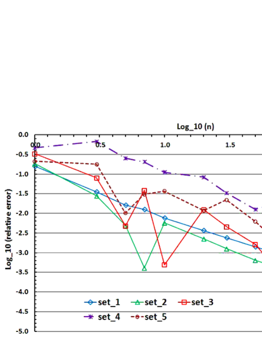
Figure 1: Empirical convergence of the proposed scheme for (6.2) with ${\rm set}_{i},i\in\{1,\cdots,5\}$.

We have tested the following five sets of parameters $(\sigma_{i=1,2},a)$:

$${\rm set}_{1}=\bigl{\{}\sigma_{i}=0.5,a=1.0\bigr{\}},~{}{\rm set}_{2}=\bigl{\{}\sigma_{i}=0.5,a=2.0\bigr{\}},~{}{\rm set}_{3}=\bigl{\{}\sigma_{i}=0.5,a=3.0\bigr{\}},$$

$${\rm set}_{4}=\bigl{\{}\sigma_{i}=1.0,a=3.0\bigr{\}},~{}{\rm set}_{5}=\bigl{\{}\sigma_{i}=0.5,a=4.0\bigr{\}}$$ (6.5)

by changing the partition from $n=1$ to $n=300$. In Figure 1, we have plotted $\log_{10}$(relative error) against the $\log_{10}(n)$ for set${}_{i},i\in\{1,\cdots,5\}$, where the relative error is defined by

$$\frac{\mbox{estimated $Y_{0}$ by the proposed scheme}-\mbox{the value obtained from (\ref{eq-closed})}}{\mbox{the value obtained from (\ref{eq-closed})}}~{}.$$

As naturally expected, the bigger “$a$” we use, the bigger $\zeta$ is needed to keep the derivatives (calculated by finite-difference scheme) non-divergent as Assumption 5.1 requires.

Driver truncation

As we have emphasized, it is crucial to have stable derivatives as Assumption 5.1 for the proposed scheme to converge. For the qg-BSDE (6.2), if we increase the coefficient “$a$” while keeping the factor $\zeta$ of $\Delta=\zeta|\pi|^{1/2}$ constant, we have observed that these derivatives (and hence the estimate of $Y$) are, in fact, divergent. In the remainder, instead of making $\zeta$ larger, let us study the truncation of the driver $f$ so that it has a global Lipschitz constant $N$ following the scaling rule ( see Section 2.1 of [15] )

$$N\propto n^{\alpha},\quad 0<\alpha<1~{}.$$ (6.6)

The error estimates for the qg-BSDEs under this truncation have been studied by Imkeller & Reis (2010) [33] (Theorem 6.2) and applied to the backward numerical scheme by Chassagneux & Richou (2016) [15]. From Theorem 6.2 [33], one easily sees that this truncation does not affect the theoretical bound on the convergence rate of Theorem 4.1, which is also the case for the scheme studied in [15].

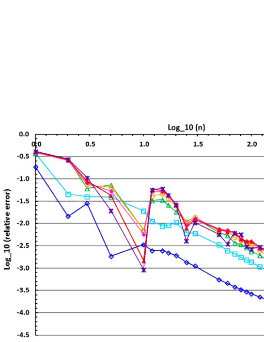
Figure 2: Empirical convergence of the proposed scheme for (6.2) with a truncated driver so that the Lipschitz constant scales as $N\propto n^{1/3}$.

We have chosen the constant $\zeta$ so that it marginally works for the $\text{set}_{3}$ in (6.5) without any truncation and adopted the scaling factor $\alpha=1/3$. We tested the following seven cases of large quadratic coefficients;

$$\{a=2,~{}a=4,~{}a=6,~{}a=8,~{}a=10,~{}a=12,~{}a=20\}$$ (6.7)

while keeping the other parameters the same, i.e.,

$$x_{0}=(1,1)^{\top},~{}T=1,~{}b_{1}=b_{2}=0.05,~{}\rho=0.3,~{}\sigma_{1}=\sigma_{2}=0.5~{}.$$ (6.8)

In Figure 2, we have plotted the $\log_{10}$(relative error) against the $\log_{10}(n)$ changing the number of partitions from $n=1$ to $n=500$. Except for coarse partitions $n\lesssim 10$, the truncation of the driver yields quite stable convergence even for very large quadratic coefficients. We find no significant change in the empirical convergence rate, and it is close to one. The introduction of the truncation $(\ref{eq-driver-truncation})$ looks quite attractive since there is no need to adjust $\zeta$ according to different size of the coefficient $a$. There seems a deep relation among the stability (Assumption 5.1), the scaling rule of finite difference scheme as well as the truncation of the driver $(N\propto n^{\alpha})$. This interesting problem requires further research.

Remark 6.1.

Since the truncation introduced in Imkeller & Reis [33] leaves the structure condition (Assumption 2.2 (i)) intact, one can still use the error estimates derived for qg-BSDEs. From Theorem 6.2 [33], one can see that the difference of the original qg-BSDE and its truncated version by the Lipschitz constant $N$ $(\delta Y:=Y-Y^{N},\delta Z^{N}:=Z-Z^{N})$ scales as $||(\delta Y^{N},\delta Z^{N})||_{{\cal K}^{p}}\propto N^{-\beta}=n^{-\alpha\beta}$ with an arbitrary $\beta>0$. Hence, it does not affect the estimate of the convergence speed. On the other hand, one cannot improve the convergence analysis by adopting the simpler proof of the Lipschitz BSDEs (see Section 6.2.1) combined with the truncation method. This is because the coefficients of the error estimates generally depend on the Lipschitz constant exponentially as $C\propto e^{NT}=e^{n^{\alpha}T}$ through the use of the Gronwall’s lemma.

Non-differentiable terminal function

We now test a case of non-differentiable terminal function

$$\xi(x)=\min\bigl{(}\max(x^{\bf{1}},1),3\bigr{)}+\max(2-x^{\bf{2}},0)~{}$$ (6.9)

in (6.2). If we apply the finite-difference scheme given in the last section directly, the 2nd and 3rd-order derivatives appearing in Assumption 5.1 grow with the rate of $1/\Delta$ and $1/\Delta^{2}$, at least, near the boundary $t=T$. Thus one naturally expects some instability appears if the space discretization $\Delta=\zeta|\pi|^{1/2}$ becomes sufficiently small. Note that, one can always apply the technique of Section 5 as long as an appropriate mollified function is chosen and kept fixed. In this case, however, the total error of Corollary 5.1 contains, of course, an additional term arising from the mollification.

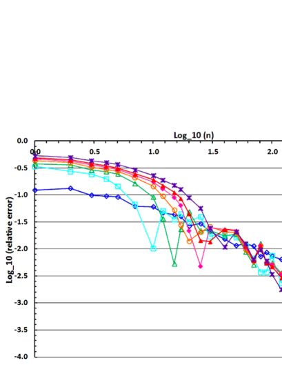
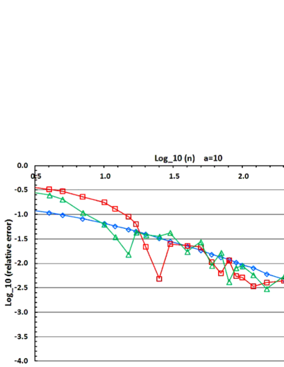
Figure 3: Empirical convergence of the proposed scheme for (6.2) with a non-differentiable terminal function (6.9). The left one uses (6.8) with $a$’s in (6.7), and the right one uses $a=10$ and (6.8) but with difference choices of volatilities $(\sigma_{i})_{1\leq i\leq 2}=0.2,~{}0.5,~{}1.0$.

In Figure 3, we have tested the model (6.2) with the terminal function (6.9) and plotted the $\log_{10}$(relative error) for the number of partitions from $n=1$ to $n=500$ by directly applying the finite-difference scheme. The same truncation of the driver $N\propto n^{1/3}$ has been used as in the previous example. In the left figure, we have tested the same seven cases of “$a$” (6.7) with the same set of parameters (6.8). In the right one, we have kept $a=10$ but tested (6.8) replaced by three different choices of volatilities $(\sigma_{i})_{1\leq i\leq 2}=0.2,~{}0.5,~{}1.0$. The results are very encouraging. From the left one, although one actually observes some instability, the overall rate of convergence is not much different from the previous example in Fig 2 of a differentiable terminal function. From the right one, one observes that the size of volatilities does not meaningfully affect the empirical convergence rate (but increases the instability to a certain degree).

In the computation, we observed that the maximum of the derivatives decays rather quickly when $t$ is away from the maturity. In fact, from the expression (6.3) and the integration-by-parts formula, one can show that the solution $Y_{t}^{t,\cdot}:\mathbb{R}^{d}\rightarrow\mathbb{R}$ is a smooth function of $x$ for $t<T$ as long as $X_{T}$ has a smooth density, which is the case for the current log-normal model (6.1) for $(X_{t})_{t\in[0,T]}$. The above numerical result (and also the examples of the next subsection) suggests relaxing the conditions in Assumptions 2.2, 3.1 (and hence 5.1) may be possible under appropriate conditions. Further studies on the regularity of the true solution as well as its approximation are needed.

6.2 Lipschitz BSDEs

6.2.1 About the convergence estimate for Lipschitz BSDEs

In the reminder, let us test the proposed scheme for a Lipschitz BSDE for completeness. The scheme given in the previous sections is equally applicable to the standard Lipschitz BSDEs and yields the same convergence estimates. Before providing the numerical results, let us briefly explain the allowed setup as well as the associated changes in the relevant results. The major changes in the setup can be summarized as follows:
$\bullet~{}$$\xi(x)$ and $f(t,x,0,0)$ have at most polynomial growth in $x$.
$\bullet~{}$$\xi\in C^{3}(\mathbb{R}^{d})$ and $f$ is one-time continuously differentiable with respect to the spatial variables $(x,y,z)$, where $|\partial_{y}f|,|\partial_{z}f|$ are bounded and $|\partial_{x}f|$ has at most polynomial growth in $x$.
$\bullet~{}$Assumption 3.1 (ii) is removed and (i) is modified as $\max_{1\leq i\leq n}|\partial_{x}^{m}\widehat{u}^{i+1}(x)|\leq K^{\prime}(1+|x|^{(\varrho-m)\vee 0}),~{}\forall x\in\mathbb{R}^{d},m=0,\cdots,3$ with some positive integer $\varrho\geq 1$. The perturbation $(\delta^{i})_{i}$ are now allowed to have polynomial growth.
$\bullet~{}$Assumption 5.1 is modified accordingly to check the above polynomial growth condition.

Note that the boundedness of the terminal function used for qg-BSDEs is needed to guarantee that the derivative process $(\partial_{x}\overline{\Theta}^{i,t,x})$ is well-posed by the results [13]. Since the derivative process $\partial_{x}\overline{\Theta}^{i,t,x}$ now follows a Lipschitz BSDE, the boundedness condition is unnecessary and similar analysis in Proposition 3.1 yields $|\overline{Z}^{i}_{t}|\leq C(1+|X_{t}|^{\varrho})$. Theorem 3.1 still holds by the same analysis. Note that $|\gamma_{t}^{i}|$ is now bounded by Lipschitz constant and hence Proposition 3.2 is unnecessary anymore. Since $X^{t,x}\in\mathbb{S}^{p}$ for any $p\geq 1$, the scaling of $h_{i}$ (such as $Ch_{i}^{3p/2}$ etc.) for the short-term expansion in the Appendixes B and C is unchanged. From these observations, one can show that the estimate in Theorem 4.1 still holds true.

Since $(|\partial_{x}^{m}\widehat{u}^{i}|)_{i,m}$ have polynomial growth, the constants $C$’s appearing in Section 5 (in particular those in Lemma 5.1 and Definition 5.1) generally depend polynomially in $x$. This induces the changes in a way that $C\Delta^{3}\rightarrow C\Delta^{3}(1+|x|^{\varrho})$. However, the effects can by absorbed by adjusting “$\rho$” used in Section 5 appropriately in every place. It is also the case for (5.3) since the initial-value dependence of the short-term expansion is at most polynomial. Proposition 5.1 becomes unnecessary (it is only for qg-BSDEs) and hence the scaling factor $\delta>0$ of the grid size $M$ is not restricted to $\delta<1/\rho$. Proposition 5.2 is proved exactly the same manner with the modified $\rho$ and Corollary 5.1, which is the main result, is shown to hold by simple application of Chebyshev’s inequality.

6.2.2 Numerical examples: Option pricing with different interest rates

We use the same scaling rule $\Delta=\zeta|\pi|^{1/2}$ but, of course, no truncation of the driver. We consider a very popular valuation problem of European options under two different interest rates, $r$ for investing and $R~{}(\neq r)$ for borrowing. Since this problem has been often used for testing the numerical schemes for Lipschitz BSDEs, it would be informative to compare the current scheme to the existing numerical examples based on Monte Carlo simulation.

Let us assume the dynamics of the security price as

$$X_{t}=x_{0}+\int_{0}^{t}\mu X_{s}ds+\int_{0}^{t}\sigma X_{s}dW_{s}~{},$$

where $d=1$ and $\mu,\sigma$ are positive constants. For the option payoff $\Phi(X_{T})$ at the expiry $T$, the option price $Y_{t}$ implied by the self-financing replication is given by

$$Y_{t}=\Phi(X_{T})-\int_{t}^{T}\Bigl{\{}rY_{s}+\frac{\mu-r}{\sigma}Z_{s}-\Bigl{(}Y_{s}-\frac{Z_{s}}{\sigma}\Bigr{)}^{-}(R-r)\Bigr{\}}ds-\int_{t}^{T}Z_{s}dW_{s}~{}.$$ (6.10)

Although both the terminal and driver functions are not smooth, we can expect rather accurate results considering the result in Fig 3 for the qg-BSDE .

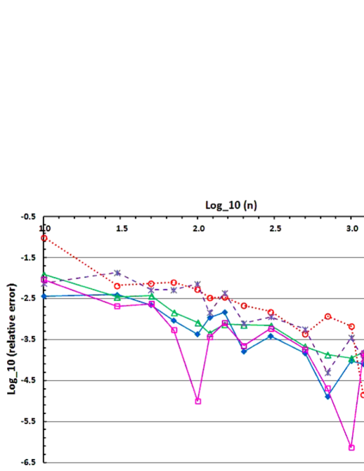
Figure 4: Empirical convergence of the proposed scheme for (6.10) for call options.

Firstly, we study the cases where the payoff function is equal to that of a call option: $\Phi(x)=(x-K)^{+}$, where $K>0$ is the strike price. As suggested by [32], this example provides a very interesting test since the price must be exactly equal to that of Black-Scholes model with interest rate $R$. This is because the replicating portfolio consists of the long-only position and hence the investor must always borrow money to fund her position. We have chosen the common parameters as $\{T=1,r=0.01,~{}R=0.06,~{}\mu=0.06,~{}X_{0}=100\}$ and tested the following five sets of $(K,\sigma)$  with $n=10$ to $n=3000$ in Figure 4:

$${\rm set}_{1}=\{K=106,~{}\sigma=0.3\}~{},{\rm set}_{2}=\{K=166,~{}\sigma=0.3\}~{},{\rm set}_{3}=\{K=106,~{}\sigma=1.0\}~{},$$

$${\rm set}_{4}=\{K=306,~{}\sigma=1.0\}~{},{\rm set}_{5}=\{K=106,~{}\sigma=2.0\}.$$

The Black-Scholes price for each set is given by ${\rm BS}=\{12.000,1.117,38.346,11.662,68.296\}$ respectively. Although the relative errors for OTM options are slightly higher, the convergence rate to the exact BS prices is close to 1 for every case. It is a bit striking that we do not see any deterioration in convergence rate in spite of the non-smooth functions and rather high volatilities. The observed irregularity of the error size is likely due to the change of the configuration of the grids close to the terminal time relative to the non-differentiable points of the terminal function.

Next, let us consider a call-spread case: $\Phi(x)=(x-K_{1})^{+}-2(x-K_{2})^{+}$. This is exactly the same setup studied in [32] and hence we can test the performance of our scheme relative to the standard regression-based Monte Carlo simulation. Let us choose the same parameter sets as in [32]:

$$\{r=0.01,~{}R=0.06,~{}\mu=0.05,~{}X_{0}=100,~{}T=0.25,~{}\sigma=0.2,~{}K_{1}=95,~{}K_{2}=105\}$$ (6.11)

The result of [32] suggests that $Y_{0}=2.96\pm 0.01$ or $Y_{0}=2.95\pm 0.01$ with one standard deviation dependent on the choice of basis functions for the regressions. In Figure 6, we have compared the estimated $Y_{0}$ from our scheme and the one in [32]. The dotted lines represent $2.96\pm 0.01$ for ease of comparison. In our scheme, $Y_{0}$ converges toward $2.96$. In fact, the improvement of the regression method of [32] using martingale basis functions proposed by Bender & Steiner (2012) [5] suggests $2.96$ which is perfectly consistent with our result.

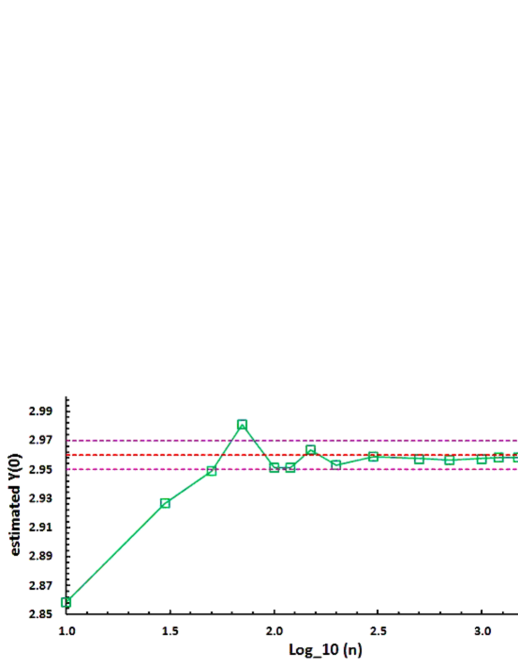
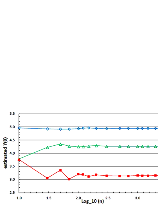
Figure 5: Empirical convergence of the proposed scheme for (6.10) for a call spread.

Figure 6: Empirical convergence of the proposed scheme for (6.10) for a call spread with $T=1.0$ and higher volatilities.

We have also tested the convergence with a longer maturity and higher volatilities for the final payoff $\Phi(x)=(x-K_{1})^{+}-(x-K_{2})^{+}$. We have used $\{r=0.01,~{}R=0.06,~{}\mu=0.05,~{}X_{0}=100,~{}K_{1}=95,~{}K_{2}=105\}$ as before, but with longer maturity $T=1.0$ and ${\rm set}_{1}:=\{\sigma=0.3\}$, ${\rm set}_{2}:=\{\sigma=0.5\}$ and ${\rm set}_{3}:=\{\sigma=1.0\}$. From Figure 6, one observes smooth convergence for all the cases. The decrease in price for higher volatilities is natural from the fact that $K_{2}$ is closer to the at-the-money-forward point and hence the short position has higher sensitivity on the volatility.

An example with a large Lipschitz constant

Bender & Steiner [5] have tested an extreme scenario with a parameter set (6.11) replaced by $R=3.01$. In this case, the non-linearity of the driver has a Lipschitz constant $(R-r)/\sigma=15$. Their experiments suggest that the standard method of [32] fails to converge for this example under the simulation settings they tried. Their improved method with martingale basis functions (see Table 3 in [5]) gives $Y_{0}\simeq 6.47$ with $n=128$ and $Y_{0}\simeq 6.44$ with the finest partition $n=181$.

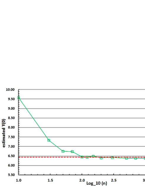
Figure 7: Empirical convergence of the proposed scheme for (6.10) with $R=3.01$.

In Figure 7, we have plotted estimated $Y_{0}$ from our scheme with $n=10$ to $n=3000$. The dotted line corresponds to the value $6.44$ given in [5]. In our scheme, $Y_{0}$ seems to converge to $6.38$. In particular, with the same discretization $n=181$, our scheme yields $Y_{0}\simeq 6.43$ showing a nice consistency. Note that the method [5] requires to change the basis functions based on the law of $X$.

Remark 6.2.

Our numerical computation is implemented in Microsoft Excel VBA with Xeon X5570 cpu @ 2.93GHz. It takes around $8$ seconds for $2$-dimensional examples of qg-BSDE with $n=100$ time steps, and about $0.8$ seconds for $1$-dimensional examples of Lipschitz BSDE with $n=1000$ time steps.

7 Conclusion

In this paper, we have developed a semi-analytic computation scheme for Markovian qg-BSDEs by connecting the short-term expansions that are given in explicit form by the asymptotic expansion technique. The method can be applied also to the standard Lipschitz BSDEs in almost the same way. At least for low dimensional setups, the scheme is quite easy to implement as a slightly elaborated tree method and has high accuracy even for very large quadratic coefficients and Lipschitz constants. For high-dimensional setups, we have suggested a sparse grid scheme as a promising candidate to overcome the curse-of-dimensionality at least to a certain degree. Testing this interesting idea is left for future work.

From a theoretical viewpoint, the main difficulty has arisen from controlling the bound of the derivatives $|\partial_{x}^{m}\widehat{u}^{i}|$ uniformly, which remains as an open question. This forces us to require a posteriori checks for these bounds as in Assumption 5.1 to guarantee the convergence for a given range. Under appropriate assumptions, the properties of the corresponding semilinear PDEs may provide the necessary regularities. Pursuing this issue is left for future work.

Appendix A BMO-martingale and its properties

In this section, let us summarize the properties of BMO-martingales, the associated ${\cal H}^{2}_{BMO}$-space and their properties which play an important role in the discussions.

Definition A.1.

A BMO-martingale $M$ is a square integrable martingale satisfying $M_{0}=0$ and

$$||M||^{2}_{BMO}:=\sup_{\tau\in{\cal T}^{T}_{0}}\Bigl{|}\Bigl{|}\mathbb{E}\Bigl{[}\langle M\rangle_{T}-\langle M\rangle_{\tau}|{\cal F}_{\tau}\Bigr{]}\Bigr{|}\Bigr{|}_{\infty}<\infty~{},$$

where the supremum is taken over all stopping times $\tau\in{\cal T}^{T}_{0}$.

Definition A.2.

${\cal H}^{2}_{BMO}(\mathbb{R}^{k})$ is the set of $\mathbb{R}^{k}$-valued progressively measurable processes $Z$ satisfying

$$||Z||^{2}_{{\cal H}^{2}_{BMO}}:=\sup_{\tau\in{\cal T}^{T}_{0}}\Bigl{|}\Bigl{|}\mathbb{E}\Bigl{[}\int_{\tau}^{T}|Z_{s}|^{2}ds\Bigr{|}{\cal F}_{\tau}\Bigr{]}\Bigr{|}\Bigr{|}_{\infty}<\infty~{}.$$

Note that if $Z\in{\cal H}^{2}_{BMO}(\mathbb{R}^{1\times d})$, we have

$$\Bigl{|}\Bigl{|}\int_{0}^{\cdot}Z_{s}dW_{s}\Bigr{|}\Bigr{|}_{BMO}^{2}=\sup_{\tau\in{\cal T}^{T}_{0}}\Bigl{|}\Bigl{|}\mathbb{E}\Bigl{[}\int_{\tau}^{T}|Z_{s}|^{2}ds\Bigr{|}{\cal F}_{\tau}\Bigr{]}\Bigr{|}\Bigr{|}_{\infty}=||Z||^{2}_{{\cal H}^{2}_{BMO}}<\infty~{},$$

and hence $Z*W:=\int_{0}^{\cdot}Z_{s}dW_{s}$ is a BMO-martingale. The next result is well-known as energy inequality.

Lemma A.1.

Let $Z$ be in ${\cal H}^{2}_{BMO}$. Then, for any $n\in\mathbb{N}$,

$$\mathbb{E}\Bigl{[}\Bigl{(}\int_{0}^{T}|Z_{s}|^{2}ds\Bigr{)}^{n}\Bigr{]}\leq n!\Bigl{(}||Z||^{2}_{{\cal H}^{2}_{BMO}}\Bigr{)}^{n}~{}.$$

Proof.

See proof of Lemma 9.6.5 in [20]. ∎

Let ${\cal E}(M)$ be a Doléans-Dade exponential of $M$.

Lemma A.2.

(Reverse Hölder inequality) Let $M$ be a BMO-martingale. Then, $\bigl{(}{\cal E}_{t}(M),t\in[0,T]\bigr{)}$ is a uniformly integrable martingale, and for every stopping time $\tau\in{\cal T}^{T}_{0}$, there exists some positive constant $r^{*}>1$ such that the inequality

$$\mathbb{E}\Bigl{[}{\cal E}_{T}(M)^{r}|{\cal F}_{\tau}\Bigr{]}\leq C_{r,M}{\cal E}_{\tau}(M)^{r}~{},$$

holds for every $1<r\leq r^{*}$ with some positive constant $C_{r,M}$ depending only on $r$ and $||M||_{BMO}$.

Proof.

See Theorem 3.1 of Kazamaki (1994) [34]. ∎

Lemma A.3.

Let $M$ be a square integrable martingale and $\widehat{M}:=\langle M\rangle-M$. Then, $M\in BMO(\mathbb{P})$ if and only if $\widehat{M}\in BMO(\mathbb{Q})$ with $d\mathbb{Q}/d\mathbb{P}={\cal E}_{T}(M)$. Furthermore, $||\widehat{M}||_{BMO(\mathbb{Q})}$ is determined by some function of $||M||_{BMO(\mathbb{P})}$.

Proof.

See Theorem 2.4 and 3.3 in [34]. ∎

Remark A.1.

Theorem 3.1 [34] also tells that there exists some decreasing function $\Phi(r)$ with $\Phi(1+)=\infty$ and $\Phi(\infty)=0$ such that if $||M||_{BMO(\mathbb{P})}$ satisfies $||M||_{BMO(\mathbb{P})}<\Phi(r)$ then ${\cal E}(M)$ allows the reverse Hölder inequality with power $r$. This implies together with Lemma A.3, one can take a common positive constant $\bar{r}$ satisfying $1<\bar{r}\leq r^{*}$ such that both of the ${\cal E}(M)$ and ${\cal E}(\hat{M})$ satisfy the reverse Hölder inequality with power $\bar{r}$ under the respective probability measure $\mathbb{P}$ and $\mathbb{Q}$. Furthermore, the upper bound $r^{*}$ is determined only by $||M||_{BMO(\mathbb{P})}$ (or equivalently by $||M||_{BMO(\mathbb{Q})}$).

Appendix B Short-term expansion: Step 1

In the following two sections, we approximate the solution $(\overline{Y}^{i},\overline{Z}^{i})$ of the BSDE (3.1) semi-analytically and also obtain its error estimate. We need two steps for achieving this goal, which involve the linearization method and the small-variance expansion method for BSDEs proposed in Fujii & Takahashi (2012) [27] and (2015) [31], respectively .

When there is no confusion, we adopt the so-called Einstein convention assuming the obvious summation of duplicate indexes (such as $i\in\{1,\cdots,d\}$ of $x^{i}$) without explicitly using the summation symbol $\sum$. For example, $\partial_{x^{i},x^{j}}\xi(X_{T})\partial_{x}X_{T}^{i}\partial_{x}X_{T}^{j}$ assumes the summation about indexes $i$ and $j$ so that it denotes $\sum_{i,j=1}^{d}\partial_{x^{i},x^{j}}\xi(X_{T})\partial_{x}X_{T}^{i}\partial_{x}X_{T}^{j}$.

(Standing Assumptions for Section B) We make Assumptions 2.1, 2.2 and Assumption 3.1 (i) the standing assumptions for this section.

Let us introduce the next decomposition of the BSDE (3.1) for each interval $t\in I_{i}$, $i\in\{1,\cdots,n\}$:

$$\overline{Y}_{t}^{i,[0]}=\widehat{u}^{i+1}(X_{t_{i}})-\int_{t}^{t_{i}}\overline{Z}_{r}^{i,[0]}dW_{r}~{},$$ (B.1)

$$\overline{Y}_{t}^{i,[1]}=\int_{t}^{t_{i}}f\bigl{(}r,X_{r},\overline{Y}^{i,[0]}_{r},\overline{Z}_{r}^{i,[0]}\bigr{)}dr-\int_{t}^{t_{i}}\overline{Z}_{r}^{i,[1]}dW_{r}~{}.$$ (B.2)

They are the leading contributions in the linearization method [27, 48].

Lemma B.1.

For every interval $I_{i},i\in\{1,\cdots,n\}$, there exists a unique solution $(\overline{Y}^{i,[0]},\overline{Z}^{i,[0]})$ to the BSDE (B.1) satisfying, with some $(i,n)$-independent positive constants $C$ and $C_{p}$, that $\displaystyle||\overline{Y}^{i,[0]}||_{{\cal S}^{\infty}[t_{i-1},t_{i}]}+||\overline{Z}^{i,[0]}||_{{\cal H}^{2}_{BMO}[t_{i-1},t_{i}]}\leq C$, and also $||\overline{Z}^{i,[0]}||_{{\cal S}^{p}[t_{i-1},t_{i}]}\leq C_{p}$ for any $p\geq 2$.

Proof.

The boundedness $||\overline{Y}^{i,[0]}||_{{\cal S}^{\infty}}\leq C$ follows easily from Assumption 3.1 (i), which then implies $||\overline{Z}^{i,[0]}||_{{\cal H}^{2}_{BMO}}\leq C$. The second claim follows from the similar arguments used in Proposition 3.1 . ∎

Lemma B.2.

For every interval $I_{i}$, $i\in\{1,\cdots,n\}$, there exists a unique solution $(\overline{Y}^{i,[1]},\overline{Z}^{i,[1]})$ to the BSDE (B.2) satisfying, with some $(i,n)$-independent positive constant $C_{p}$, that

$$||\overline{Y}^{i,[1]}||_{{\cal S}^{p}[t_{i-1},t_{i}]}+||\overline{Z}^{i,[1]}||_{{\cal H}^{p}[t_{i-1},t_{i}]}\leq C_{p}$$

for any $p\geq 2$.

Proof.

Since it is a Lipschitz BSDE (with zero Lipschitz constant), the existence of a unique solution easily follows. The standard estimate (see, for example, [12]) and Assumption 2.2 (i) implies

$$\Bigl{|}\Bigl{|}(\overline{Y}^{i,[1]},\overline{Z}^{i,[1]})\Bigr{|}\Bigr{|}^{p}_{{\cal K}^{p}[t_{i-1},t_{i}]}\leq C_{p}\mathbb{E}\Bigl{[}\Bigl{(}\int_{t_{i-1}}^{t_{i}}|f(r,X_{r},\overline{Y}_{r}^{i,[0]},\overline{Z}_{r}^{i,[0]})|dr\Bigr{)}^{p}\Bigr{]}$$

$$\qquad\leq C_{p}\mathbb{E}\Bigl{[}\Bigl{(}\int_{t_{i-1}}^{t_{i}}\bigl{[}l_{r}+\beta|\overline{Y}^{i,[0]}_{r}|+\frac{\gamma}{2}|\overline{Z}_{r}^{i,[0]}|^{2}\bigr{]}dr\Bigr{)}^{p}\Bigr{]}$$

$$\qquad\leq C_{p}\Bigl{(}||l||^{p}_{T}+||\overline{Y}^{i,[0]}||^{p}_{{\cal S}^{p}[t_{i-1},t_{i}]}+||\overline{Z}^{i,[0]}||^{2p}_{{\cal S}^{2p}[t_{i-1},t_{i}]}\Bigr{)}~{}.$$

Thus one obtains the desired result by Lemma B.1. ∎

We now define the process $(\widetilde{\overline{Y}}^{i},\widetilde{\overline{Z}}^{i})$ for each interval $t\in I_{i}$, $i\in\{1,\cdots,n\}$ by

$$\widetilde{\overline{Y}}^{i}_{t}:=\overline{Y}^{i,[0]}_{t}+\overline{Y}_{t}^{i,[1]}~{},\qquad\widetilde{\overline{Z}}^{i}_{t}:=\overline{Z}^{i,[0]}_{t}+\overline{Z}_{t}^{i,[1]}~{}.$$

Proposition B.1.

There exists some $(i,n)$-independent positive constant $C_{p}$ such that the inequality

$$\mathbb{E}\Bigl{[}\bigl{|}\bigl{|}\overline{Y}^{i}-\widetilde{\overline{Y}}^{i}\bigr{|}\bigr{|}^{p}_{[t_{i-1},t_{i}]}+\Bigl{(}\int_{t_{i-1}}^{t_{i}}\bigl{|}\overline{Z}_{r}^{i}-\widetilde{\overline{Z}}^{i}_{r}\bigr{|}^{2}dr\Bigr{)}^{\frac{p}{2}}\Bigr{]}\leq C_{p}h_{i}^{3p/2}$$

holds for every interval $I_{i}$, $i\in\{1,\cdots,n\}$ with any $p\geq 2$.

Proof.

For notational simplicity, let us put

$$\delta Y^{i,[0]}_{t}:=\overline{Y}^{i}_{t}-\overline{Y}^{i,[0]}_{t},\quad\delta Z^{i,[0]}_{t}:=\overline{Z}^{i}_{t}-\overline{Z}_{t}^{i,[0]}$$

$$\delta Y^{i,[1]}_{t}:=\overline{Y}^{i}_{t}-\widetilde{\overline{Y}}^{i}_{t},\qquad\delta Z^{i,[1]}_{t}:=\overline{Z}^{i}_{t}-\widetilde{\overline{Z}}^{i}_{t}~{}$$

for each interval $t\in I_{i},i\in\{1,\cdots,n\}$. Then, they are given by the solutions to the following BSDEs respectively:

$$\delta Y^{i,[0]}_{t}=\int_{t}^{t_{i}}f(r,X_{r},\overline{Y}^{i}_{r},\overline{Z}_{r}^{i})dr-\int_{t}^{t_{i}}\delta Z^{i,[0]}_{r}dW_{r}~{},$$

$$\delta Y^{i,[1]}_{t}=\int_{t}^{t_{i}}\Bigl{(}f(r,X_{r},\overline{Y}^{i}_{r},\overline{Z}_{r}^{i})-f(r,X_{r},\overline{Y}^{i,[0]}_{r},\overline{Z}_{r}^{i,[0]})\Bigr{)}dr-\int_{t}^{t_{i}}\delta Z_{r}^{i,[1]}dW_{r}~{}.$$

By the stability result for the Lipschitz BSDEs (see, for example, [12]), Assumption 2.2 (i), (3.3) and Proposition 3.1, one obtains

$$\Bigl{|}\Bigl{|}(\delta Y^{i,[0]},\delta{Z}^{i,[0]})\Bigr{|}\Bigr{|}^{p}_{{\cal K}^{p}[t_{i-1},t_{i}]}\leq C_{p}\mathbb{E}\Bigl{[}\Bigl{(}\int_{t_{i-1}}^{t_{i}}\bigl{[}l_{r}+\beta|\overline{Y}^{i}_{r}|+\frac{\gamma}{2}|\overline{Z}_{r}^{i}|^{2}\bigr{]}dr\Bigr{)}^{p}\Bigr{]}$$

$$\qquad\leq C_{p}h_{i}^{p}\left(||l||_{T}^{p}+||\overline{Y}^{i}||_{{\cal S}^{\infty}[t_{i-1},t_{i}]}^{p}+||\overline{Z}^{i}||^{2p}_{{\cal S}^{2p}[t_{i-1},t_{i}]}\right)\leq C_{p}h_{i}^{p},$$ (B.3)

with some $(i,n)$-independent positive constant $C_{p}$ for $\forall p\geq 2$. Similar analysis for $(\delta Y^{i,[1]},\delta Z^{i,[1]})$ using Assumption 2.2 (ii) yields

$$\Bigl{|}\Bigl{|}(\delta Y^{i,[1]},\delta{Z}^{i,[1]})\Bigr{|}\Bigr{|}^{p}_{{\cal K}^{p}[t_{i-1},t_{i}]}\leq C_{p}\mathbb{E}\Bigl{[}\Bigl{(}\int_{t_{i-1}}^{t_{i}}\Bigl{[}|\delta Y^{i,[0]}_{r}|+(1+|\overline{Z}_{r}^{i}|+|\overline{Z}_{r}^{i,[0]}|)|\delta Z_{r}^{i,[0]}|\Bigr{]}dr\Bigr{)}^{p}\Bigr{]}$$

$$\quad\leq C_{p}\Bigl{(}h_{i}^{p}||\delta Y^{i,[0]}||^{p}_{{\cal S}^{p}[I_{i}]}+\mathbb{E}\Bigl{[}1+||\overline{Z}^{i}||^{2p}_{I_{i}}+||\overline{Z}^{i,[0]}||^{2p}_{I_{i}}\Bigr{]}^{\frac{1}{2}}\mathbb{E}\Bigl{[}\Bigl{(}h_{i}\int_{t_{i-1}}^{t_{i}}|\delta Z_{r}^{i,[0]}|^{2}dr\Bigr{)}^{p}\Bigr{]}^{\frac{1}{2}}\Bigr{)}.$$

By applying Proposition 3.1, Lemma B.1 and the previous estimate (B.3), one obtains the desired result. ∎

Appendix C Short-term expansion: Step 2

In the second step, we obtain simple analytic approximation for the BSDEs (B.1) and (B.2) while keeping the same order of accuracy given in Proposition B.1. We use the small-variance expansion method for BSDEs proposed in [31] which renders all the problems into a set of simple ODEs. Furthermore, we shall see that these ODEs can be approximated by a single-step Euler method for each interval $I_{i}$.

(Standing Assumptions for Section C) Similarly to the last section, we make Assumptions 2.1, 2.2 and Assumption 3.1 (i) the standing assumptions for this section.

C.1 Approximation for $(\overline{Y}^{i,[0]},\overline{Z}^{i,[0]})$

For each interval, we introduce a new parameter $\epsilon$ satisfying $\epsilon\in(-c,c)$ with some constant $c>1$ to perturb (2.1) and (B.1):

$$X_{t}^{\epsilon}=X_{t_{i-1}}+\int_{t_{i-1}}^{t}b(r,X_{r}^{\epsilon})dr+\int_{t_{i-1}}^{t}\epsilon\sigma(r,X_{r}^{\epsilon})dW_{r}~{}.$$ (C.1)

$$\overline{Y}_{t}^{i,[0],\epsilon}=\widehat{u}^{i+1}(X_{t_{i}}^{\epsilon})-\int_{t}^{t_{i}}\overline{Z}_{r}^{i,[0],\epsilon}dW_{r}~{}.$$ (C.2)

for $t\in I_{i}=[t_{i-1},t_{i}]$, $i\in\{1,\cdots,n\}$. Notice the way $\epsilon$ is introduced to $X^{\epsilon}$, by which we have a different process for each interval $I_{i}$. In the following, in order to avoid confusion between the index specifying the interval and the one for the component of $x\in\mathbb{R}^{d}$, we use the bold Gothic symbols such as $\{\mathbb{i},\mathbb{j},\cdots\}$ for the latter, each of which runs through $1$ to $d$.

Lemma C.1.

The classical derivatives of $(X^{\epsilon},\overline{Y}^{i,[0],\epsilon},\overline{Z}^{i,[0],\epsilon})$ with respect to $\epsilon$

$$\partial_{\epsilon}^{k}X^{\epsilon}_{t}:=\frac{\partial^{k}}{\partial\epsilon^{k}}X_{t}^{\epsilon},\quad\partial_{\epsilon}^{k}\overline{Y}^{i,[0],\epsilon}:=\frac{\partial^{k}}{\partial\epsilon^{k}}\overline{Y}^{i,[0],\epsilon}_{t},\quad\partial_{\epsilon}^{k}\overline{Z}^{i,[0],\epsilon}:=\frac{\partial^{k}}{\partial\epsilon^{k}}\overline{Z}^{i,[0],\epsilon}_{t}$$

for $k=\{1,2,3\}$ are given by the solutions to the following forward- and backward-SDEs:

$$\partial_{\epsilon}X_{t}^{\epsilon,{\mathbb{i}}}=\int_{t_{i-1}}^{t}\partial_{x^{\mathbb{j}}}b^{{\mathbb{i}}}(r,X_{r}^{\epsilon})\partial_{\epsilon}X_{r}^{\epsilon,{\mathbb{j}}}dr+\int_{t_{i-1}}^{t}\bigl{[}\sigma^{{\mathbb{i}}}(r,X_{r}^{\epsilon})+\epsilon(\partial_{\epsilon}X_{r}^{\epsilon,{\mathbb{j}}})\partial_{x^{\mathbb{j}}}\sigma^{{\mathbb{i}}}(r,X_{r}^{\epsilon})\bigr{]}dW_{r}~{},$$

$$\partial_{\epsilon}^{2}X_{t}^{\epsilon,{\mathbb{i}}}=\int_{t_{i-1}}^{t}\bigl{[}\partial_{x^{\mathbb{j}}}b^{{\mathbb{i}}}(r,X_{r}^{\epsilon})\partial_{\epsilon}^{2}X_{r}^{\epsilon,{\mathbb{j}}}+\partial^{2}_{x^{\mathbb{j}},x^{\mathbb{k}}}b^{\mathbb{i}}(r,X_{r}^{\epsilon})\partial_{\epsilon}X_{r}^{\epsilon,{\mathbb{j}}}\partial_{\epsilon}X_{r}^{\epsilon,{\mathbb{k}}}\bigr{]}dr$$

$$\hskip 14.22636pt+\int_{t_{i-1}}^{t}\bigl{[}2(\partial_{\epsilon}X_{r}^{\epsilon,{\mathbb{j}}})\partial_{x^{\mathbb{j}}}\sigma^{{\mathbb{i}}}(r,X_{r}^{\epsilon})+\epsilon(\partial_{\epsilon}^{2}X_{r}^{\epsilon,{\mathbb{j}}})\partial_{x^{\mathbb{j}}}\sigma^{\mathbb{i}}(r,X_{r}^{\epsilon})+\epsilon(\partial_{\epsilon}X_{r}^{\epsilon,{\mathbb{j}}})(\partial_{\epsilon}X_{r}^{\epsilon,{\mathbb{k}}})\partial^{2}_{x^{\mathbb{j}},x^{\mathbb{k}}}\sigma^{\mathbb{i}}(r,X_{r}^{\epsilon})\bigr{]}dW_{r}~{},$$

$$\partial_{\epsilon}^{3}X_{t}^{\epsilon,{\mathbb{i}}}=\int_{t_{i-1}}^{t}\bigl{[}\partial_{x^{\mathbb{j}}}b^{\mathbb{i}}(r,X_{r}^{\epsilon})\partial_{\epsilon}^{3}X_{r}^{\epsilon,{\mathbb{j}}}+3\partial^{2}_{x^{\mathbb{j}},x^{\mathbb{k}}}b^{{\mathbb{i}}}(r,X_{r}^{\epsilon})\partial^{2}_{\epsilon}X_{r}^{\epsilon,{\mathbb{j}}}\partial_{\epsilon}X_{r}^{\epsilon,{\mathbb{k}}}$$

$$\hskip 22.76219pt+\partial^{3}_{x^{\mathbb{j}},x^{\mathbb{k}},x^{\mathbb{m}}}b^{\mathbb{i}}(r,X_{r}^{\epsilon})\partial_{\epsilon}X_{r}^{\epsilon,{\mathbb{j}}}\partial_{\epsilon}X_{r}^{\epsilon,{\mathbb{k}}}\partial_{\epsilon}X_{r}^{\epsilon,{\mathbb{m}}}\bigr{]}dr+\int_{t_{i-1}}^{t}\bigl{[}3(\partial_{\epsilon}^{2}X_{r}^{\epsilon,{\mathbb{j}}})\partial_{x^{\mathbb{j}}}\sigma^{\mathbb{i}}(r,X_{r}^{\epsilon})$$

$$\hskip 22.76219pt+3(\partial_{\epsilon}X_{r}^{\epsilon,{\mathbb{j}}})(\partial_{\epsilon}X_{r}^{\epsilon,{\mathbb{k}}})\partial^{2}_{x^{\mathbb{j}},x^{\mathbb{k}}}\sigma^{\mathbb{i}}(r,X_{r}^{\epsilon})+\epsilon(\partial_{\epsilon}^{3}X_{r}^{\epsilon,{\mathbb{j}}})\partial_{x^{\mathbb{j}}}\sigma^{\mathbb{i}}(r,X_{r}^{\epsilon})$$

$$\hskip 22.76219pt+3\epsilon(\partial_{\epsilon}^{2}X_{r}^{\epsilon,{\mathbb{j}}})(\partial_{\epsilon}X_{r}^{\epsilon,{\mathbb{k}}})\partial^{2}_{x^{\mathbb{j}},x^{\mathbb{k}}}\sigma^{\mathbb{i}}(r,X_{r}^{\epsilon})+\epsilon(\partial_{\epsilon}X_{r}^{\epsilon,{\mathbb{j}}})(\partial_{\epsilon}X_{r}^{\epsilon,{\mathbb{k}}})(\partial_{\epsilon}X_{r}^{\epsilon,{\mathbb{m}}})\partial^{3}_{x^{\mathbb{j}},x^{{\mathbb{k}}},x^{\mathbb{m}}}\sigma^{\mathbb{i}}(r,X_{r}^{\epsilon})\bigr{]}dW_{r}~{},$$

$$\partial_{\epsilon}\overline{Y}_{t}^{i,[0],\epsilon}=\partial_{x^{\mathbb{j}}}\widehat{u}^{i+1}(X_{t_{i}}^{\epsilon})\partial_{\epsilon}X_{t_{i}}^{\epsilon,{\mathbb{j}}}-\int_{t}^{t_{i}}\partial_{\epsilon}\overline{Z}_{r}^{i,[0],\epsilon}dW_{r}~{},$$

$$\partial_{\epsilon}^{2}\overline{Y}_{t}^{i,[0],\epsilon}=\partial_{x^{\mathbb{j}}}\widehat{u}^{i+1}(X_{t_{i}}^{\epsilon})\partial_{\epsilon}^{2}X_{t_{i}}^{\epsilon,{\mathbb{j}}}+\partial^{2}_{x^{\mathbb{j}},x^{\mathbb{k}}}\widehat{u}^{i+1}(X_{t_{i}}^{\epsilon})\partial_{\epsilon}X_{t_{i}}^{\epsilon,{\mathbb{j}}}\partial_{\epsilon}X_{t_{i}}^{\epsilon,{\mathbb{k}}}-\int_{t}^{t_{i}}\partial^{2}_{\epsilon}\overline{Z}_{r}^{i,[0],\epsilon}dW_{r}~{},$$

$$\partial_{\epsilon}^{3}\overline{Y}_{t}^{i,[0],\epsilon}=\partial_{x^{\mathbb{j}}}\widehat{u}^{i+1}(X_{t_{i}}^{\epsilon})\partial_{\epsilon}^{3}X_{t_{i}}^{\epsilon,{\mathbb{j}}}+3\partial^{2}_{x^{\mathbb{j}},x^{\mathbb{k}}}\widehat{u}^{i+1}(X_{t_{i}}^{\epsilon})(\partial_{\epsilon}^{2}X_{t_{i}}^{\epsilon,{\mathbb{j}}})(\partial_{\epsilon}X_{t_{i}}^{\epsilon,{\mathbb{k}}})$$

$$\hskip 42.67912pt+\partial^{3}_{x^{\mathbb{j}},x^{\mathbb{k}},x^{\mathbb{m}}}\widehat{u}^{i+1}(X_{t_{i}}^{\epsilon})(\partial_{\epsilon}X_{t_{i}}^{\epsilon,{\mathbb{j}}})(\partial_{\epsilon}X_{t_{i}}^{\epsilon,{\mathbb{k}}})(\partial_{\epsilon}X_{t_{i}}^{\epsilon,{\mathbb{m}}})-\int_{t}^{t_{i}}\partial_{\epsilon}^{3}\overline{Z}_{r}^{i,[0],\epsilon}dW_{r}~{},$$

for $t\in I_{i}=[t_{i-1},t_{i}]$. Einstein convention is used with $\{{\mathbb{i}},{\mathbb{j}},\cdots\}$ running through $1$ to $d$.

Proof.

The classical differentiability can be shown by following the arguments of Theorem 3.1 in [40]. See Section 6 of [31] for more details. ∎

Lemma C.2.

For $k=\{1,2,3\}$, there exists some $(i,n)$-independent positive constant $C_{p,k}$ such that the inequality

$$\mathbb{E}\Bigl{[}\bigl{|}\bigl{|}\partial_{\epsilon}^{k}X^{\epsilon}\bigr{|}\bigr{|}_{[t_{i-1},t_{i}]}^{p}\Bigr{]}\leq C_{p,k}h_{i}^{kp/2}$$

holds for every interval $I_{i},~{}i\in\{1,\cdots,n\}$ with any $p\geq 2$.

Proof.

This can be shown by applying the standard estimates for the Lipschitz SDEs given, for example, in Appendix A of [31]. For $k=1$,

$$\mathbb{E}\Bigl{[}||\partial_{\epsilon}X^{\epsilon}||_{[t_{i-1},t_{i}]}^{p}\Bigr{]} \leq C_{p}\mathbb{E}\Bigl{[}\Bigl{(}\int_{t_{i-1}}^{t_{i}}|\sigma(r,X_{r}^{\epsilon})|^{2}dr\Bigr{)}^{p/2}\Bigr{]}\leq C_{p}h_{i}^{p/2}~{}.$$

For $k=2$, one obtains

$$\mathbb{E}\Bigl{[}||\partial_{\epsilon}^{2}X^{\epsilon}||_{[t_{i-1},t_{i}]}^{p}\Bigr{]}\leq C_{p}\mathbb{E}\Bigl{[}\Bigl{(}\int_{t_{i-1}}^{t_{i}}|\partial_{\epsilon}X_{r}^{\epsilon}|^{2}dr\Bigr{)}^{p}+\Bigl{(}\int_{t_{i-1}}^{t_{i}}\bigl{[}|\partial_{\epsilon}X_{r}^{\epsilon}|^{2}+|\partial_{\epsilon}X_{r}^{\epsilon}|^{4}\bigr{]}dr\Bigr{)}^{\frac{p}{2}}\Bigr{]}$$

$$\quad\leq C_{p}\left(h_{i}^{p}\mathbb{E}\Bigl{[}||\partial_{\epsilon}X^{\epsilon}||^{2p}_{I_{i}}\Bigr{]}+h_{i}^{p/2}\mathbb{E}\Bigl{[}||\partial_{\epsilon}X^{\epsilon}||^{p}_{I_{i}}+||\partial_{\epsilon}X^{\epsilon}||^{2p}_{I_{i}}\Bigr{]}\right)\leq C_{p}h_{i}^{p}~{},$$

as desired. One can show the last case $k=3$ in a similar manner. ∎

Let introduce the following processes, with $k\in\{0,1,2\}$,

$$X_{t}^{[k]}:=\frac{\partial^{k}}{\partial\epsilon^{k}}X_{t}^{\epsilon}\Bigr{|}_{\epsilon=0},~{}\overline{Y}_{t}^{i,[0],[k]}:=\frac{\partial^{k}}{\partial\epsilon^{k}}\overline{Y}_{t}^{i,[0],\epsilon}\Bigr{|}_{\epsilon=0},\quad\overline{Z}_{t}^{i,[0],[k]}:=\frac{\partial^{k}}{\partial\epsilon^{k}}\overline{Z}_{t}^{i,[0],\epsilon}\Bigr{|}_{\epsilon=0}$$

and also

$$\widetilde{\overline{Y}}^{i,[0]}_{t}:=\sum_{k=0}^{2}\frac{1}{k!}\overline{Y}_{t}^{i,[0],[k]},\quad\widetilde{\overline{Z}}^{i,[0]}_{t}:=\sum_{k=0}^{2}\frac{1}{k!}\overline{Z}_{t}^{i,[0],[k]}$$ (C.3)

for each interval $t\in I_{i},~{}i\in\{1,\cdots,n\}$.

Lemma C.3.

There exists some $(i,n)$-independent positive constant $C_{p}$ such that the inequality

$$\mathbb{E}\Bigl{[}\bigl{|}\bigl{|}\overline{Y}^{i,[0]}-\widetilde{\overline{Y}}^{i,[0]}\bigr{|}\bigr{|}_{[t_{i-1},t_{i}]}^{p}+\Bigl{(}\int_{t_{i-1}}^{t_{i}}|\overline{Z}_{r}^{i,[0]}-\widetilde{\overline{Z}}_{r}^{i,[0]}|^{2}dr\Bigr{)}^{p/2}\Bigr{]}\leq C_{p}h_{i}^{3p/2}$$

holds for every interval $I_{i},i\in\{1,\cdots,n\}$ with any $p\geq 2$.

Proof.

We can use the residual formula of Taylor expansion thanks to the classical differentiability of $\overline{\Theta}^{i,[0],\epsilon}$ with respect to $\epsilon$;

$$\mathbb{E}\Bigl{[}\bigl{|}\bigl{|}\overline{Y}^{i,[0]}-\widetilde{\overline{Y}}^{i,[0]}\bigr{|}\bigr{|}_{[t_{i-1},t_{i}]}^{p}+\Bigl{(}\int_{t_{i-1}}^{t_{i}}|\overline{Z}_{r}^{i,[0]}-\widetilde{\overline{Z}}_{r}^{i,[0]}|^{2}dr\Bigr{)}^{p/2}\Bigr{]}$$

$$\quad\leq C_{p}\mathbb{E}\Bigl{[}\sup_{r\in I_{i}}\Bigl{|}\frac{1}{2}\int_{0}^{1}(1-\epsilon)^{2}\partial_{\epsilon}^{3}\overline{Y}^{i,[0],\epsilon}_{r}d\epsilon\Bigl{|}^{p}+\Bigl{(}\int_{t_{i-1}}^{t_{i}}\Bigl{|}\frac{1}{2}\int_{0}^{1}(1-\epsilon)^{2}\partial_{\epsilon}^{3}\overline{Z}_{r}^{i,[0],\epsilon}d\epsilon\Bigr{|}^{2}dr\Bigr{)}^{p/2}\Bigr{]}$$

$$\quad\leq C_{p}\int_{0}^{1}\Bigr{(}\mathbb{E}\Bigr{[}\bigl{|}\bigl{|}\partial_{\epsilon}^{3}\overline{Y}^{i,[0],\epsilon}\bigr{|}\bigr{|}^{p}_{[t_{i-1},t_{i}]}+\Bigl{(}\int_{t_{i-1}}^{t_{i}}\bigl{|}\partial_{\epsilon}^{3}\overline{Z}_{r}^{i,[0],\epsilon}\bigr{|}^{2}dr\Bigr{)}^{p/2}\Bigr{]}\Bigr{)}d\epsilon~{}.$$

Applying the standard estimates of the Lipschitz BSDEs (see, for example, [12]), the boundedness of $\partial_{x}^{k}\widehat{u}^{i+1}$ as well as Lemma C.2, one obtains

$$\mathbb{E}\Bigl{[}\bigl{|}\bigl{|}\overline{Y}^{i,[0]}-\widetilde{\overline{Y}}^{i,[0]}\bigr{|}\bigr{|}_{[t_{i-1},t_{i}]}^{p}+\Bigl{(}\int_{t_{i-1}}^{t_{i}}\bigl{|}\overline{Z}_{r}^{i,[0]}-\widetilde{\overline{Z}}_{r}^{i,[0]}\bigr{|}^{2}dr\Bigr{)}^{p/2}\Bigr{]}$$

$$\quad\leq C_{p}\int_{0}^{1}\left(\mathbb{E}\Bigl{[}||\partial_{\epsilon}^{3}X^{\epsilon}||^{p}_{I_{i}}+||\partial_{\epsilon}^{2}X^{\epsilon}||^{p}_{I_{i}}||\partial_{\epsilon}X^{\epsilon}||^{p}_{I_{i}}+||\partial_{\epsilon}X^{\epsilon}||^{3p}_{I_{i}}\Bigr{]}\right)d\epsilon\leq C_{p}h_{i}^{3p/2}$$

as desired. ∎

The last lemma implies that it suffices to obtain $(\widetilde{\overline{Y}}^{i,[0]},\widetilde{\overline{Z}}^{i,[0]})$ for our purpose, which is the second order approximation of $(\overline{Y}^{i,[0]},\overline{Z}^{i,[0]})$. Furthermore, as we shall see next, the solution of these BSDEs can be obtained explicitly by simple ODEs thanks to the grading structure introduced by the asymptotic expansion. The relevant system of FBSDEs is summarized below:

$$X_{t}^{[0]}=X_{t_{i-1}}+\int_{t_{i-1}}^{t}b(r,X_{r}^{[0]})dr~{},$$

$$X_{t}^{[1],{\mathbb{i}}}=\int_{t_{i-1}}^{t}\partial_{x^{\mathbb{j}}}b^{{\mathbb{i}}}(r,X_{r}^{[0]})X_{r}^{[1],{\mathbb{j}}}dr+\int_{t_{i-1}}^{t}\sigma^{\mathbb{i}}(r,X_{r}^{[0]})dW_{r}~{},$$

$$X_{t}^{[2],{\mathbb{i}}}=\int_{t_{i-1}}^{t}\Bigl{(}\partial_{x^{\mathbb{j}}}b^{\mathbb{i}}(r,X_{r}^{[0]})X_{r}^{[2],{\mathbb{j}}}+\partial^{2}_{x^{\mathbb{j}},x^{\mathbb{k}}}b^{\mathbb{i}}(r,X_{r}^{[0]})X_{r}^{[1],{\mathbb{j}}}X_{r}^{[1],{\mathbb{k}}}\Bigr{)}dr+\int_{t_{i-1}}^{t}2X_{r}^{[1],{\mathbb{j}}}\partial_{x^{\mathbb{j}}}\sigma^{\mathbb{i}}(r,X_{r}^{[0]})dW_{r}~{},$$

$$\overline{Y}_{t}^{i,[0],[0]}=\widehat{u}^{i+1}(X_{t_{i}}^{[0]})-\int_{t}^{t_{i}}\overline{Z}_{r}^{i,[0],[0]}dW_{r}~{},$$ (C.4)

$$\overline{Y}_{t}^{i,[0],[1]}=\partial_{x^{\mathbb{j}}}\widehat{u}^{i+1}(X_{t_{i}}^{[0]})X_{t_{i}}^{[1],{\mathbb{j}}}-\int_{t}^{t_{i}}\overline{Z}_{r}^{i,[0],[1]}dW_{r}~{},$$ (C.5)

$$\overline{Y}_{t}^{i,[0],[2]}=\partial_{x^{\mathbb{j}}}\widehat{u}^{i+1}(X_{t_{i}}^{[0]})X_{t_{i}}^{[2],{\mathbb{j}}}+\partial^{2}_{x^{\mathbb{j}},x^{\mathbb{k}}}\widehat{u}^{i+1}(X_{t_{i}}^{[0]})X_{t_{i}}^{[1],{\mathbb{j}}}X_{t_{i}}^{[1],{\mathbb{k}}}-\int_{t}^{t_{i}}\overline{Z}_{r}^{i,[0],[2]}dW_{r}~{},$$ (C.6)

for $t\in I_{i},i\in\{1,\cdots,n\}$ with Einstein convention for $\{{\mathbb{i}},{\mathbb{j}},\cdots\}$.

Definition C.1.

(Coefficient functions)
We define the set of functions $\chi:I_{i}\times\mathbb{R}^{d}\rightarrow\mathbb{R}^{d}$,  $y:I_{i}\times\mathbb{R}^{d}\rightarrow\mathbb{R}$,  ${\mathbb{y}}^{[1]}:I_{i}\times\mathbb{R}^{d}\rightarrow\mathbb{R}^{d}$,  ${\mathbb{y}}^{[2]}:I_{i}\times\mathbb{R}^{d}\rightarrow\mathbb{R}^{d}$,   $G^{[2]}:I_{i}\times\mathbb{R}^{d}\rightarrow\mathbb{R}^{d\times d}$,  $y^{[2]}_{0}:I_{i}\times\mathbb{R}^{d}\rightarrow\mathbb{R}$ by

$$\chi(t,x):=x+\int_{t_{i-1}}^{t}b(r,\chi(r,x))dr~{},$$

$$y(t,x):=\widehat{u}^{i+1}(\chi(t_{i},x))~{},$$

$${\mathbb{y}}^{[1]}_{{\mathbb{j}}}(t,x):=\partial_{x^{\mathbb{j}}}\widehat{u}^{i+1}(\chi(t_{i},x))+\int_{t}^{t_{i}}\partial_{x^{\mathbb{j}}}b^{\mathbb{k}}(r,\chi(r,x)){\mathbb{y}}^{[1]}_{{\mathbb{k}}}(r,x)dr~{},$$

$$G^{[2]}_{{\mathbb{j}},{\mathbb{k}}}(t,x):=\partial^{2}_{x^{\mathbb{j}},x^{\mathbb{k}}}\widehat{u}^{i+1}(\chi(t_{i},x))+\int_{t}^{t_{i}}\Bigl{\{}\Bigl{(}\bigl{[}\partial_{x}b(r,\chi(r,x))\bigr{]}G^{[2]}(r,x)\Bigr{)}^{\leftrightarrow}_{{\mathbb{j}},{\mathbb{k}}}$$

$$\hskip 56.9055pt+\partial^{2}_{x^{\mathbb{j}},x^{\mathbb{k}}}b^{\mathbb{m}}(r,\chi(r,x)){\mathbb{y}}^{[2]}_{\mathbb{m}}(r,x)\Bigr{\}}dr~{},$$

$$y^{[2]}_{0}(t,x):=\int_{t}^{t_{i}}{\rm Tr}\Bigl{(}G^{[2]}(r,x)[\sigma\sigma^{\top}](r,\chi(r,x))\Bigr{)}dr~{},$$

and ${\mathbb{y}}^{[2]}={\mathbb{y}}^{[1]}$ for $(t,x)\in I_{i}\times\mathbb{R}^{d}$, $i\in\{1,\cdots,n\}$. We have used Einstein convention and the notation $\bigl{(}[\partial_{x}b(r,x)]_{{\mathbb{i}},{\mathbb{j}}}=\partial_{x^{\mathbb{i}}}b^{\mathbb{j}}(r,x),{\mathbb{i}},{\mathbb{j}}\in\{1,\cdots,d\}\bigr{)}$. We denote the symmetrization by $A^{\leftrightarrow}:=A+A^{\top}$ for a $d\times d$-matrix $A$ .

Note that the above coefficient functions are given by the ODEs for a given $x\in\mathbb{R}^{d}$ in each period. The solution of the BSDEs are expressed by these functions in the following way:

Lemma C.4.

For each period $t\in I_{i},i\in\{1,\cdots,n\}$, the solutions of the BSDEs (C.4), (C.5) and (C.6) are given by, with Einstein convention,

$$\overline{Y}^{i,[0],[0]}_{t}=y(t,X_{t_{i-1}}),\quad\overline{Z}^{i,[0],[0]}_{t}\equiv 0\qquad\text{(0-th order)}$$

$$\overline{Y}^{i,[0],[1]}_{t}={\mathbb{y}}^{[1]}_{{\mathbb{j}}}(t,X_{t_{i-1}})X_{t}^{[1],{\mathbb{j}}},\quad\overline{Z}^{i,[0],[1]}_{t}={\mathbb{y}}^{[1]}_{{\mathbb{j}}}(t,X_{t_{i-1}})\sigma^{\mathbb{j}}(t,\chi(t,X_{t_{i-1}})),\quad\text{(1st order)}$$

and lastly, for the 2nd order

$$\overline{Y}^{i,[0],[2]}_{t}={\mathbb{y}}^{[2]}_{{\mathbb{j}}}(t,X_{t_{i-1}})X_{t}^{[2],{\mathbb{j}}}+G^{[2]}_{{\mathbb{j}},{\mathbb{k}}}(t,X_{t_{i-1}})X_{t}^{[1],{\mathbb{j}}}X_{t}^{[1],{\mathbb{k}}}+y^{[2]}_{0}(t,X_{t_{i-1}})~{},$$

$$\overline{Z}^{i,[0],[2]}_{t}=2\Bigl{(}{\mathbb{y}}^{[2]}_{\mathbb{j}}(t,X_{t_{i-1}})X_{t}^{[1],{\mathbb{k}}}\partial_{x^{\mathbb{k}}}\sigma^{\mathbb{j}}(t,\chi(t,X_{t_{i-1}}))+G^{[2]}_{{\mathbb{j}},{\mathbb{k}}}(t,X_{t_{i-1}})X_{t}^{[1],{\mathbb{j}}}\sigma^{\mathbb{k}}(t,\chi(t,X_{t_{i-1}}))\Bigr{)}~{}.$$

Proof.

This is a special case of the results of Section 8 of [31]. The existence of the unique solution to the BSDEs (C.4), (C.5) and (C.6) is obvious. The expression can be directly checked by applying Itô formula to the suggested forms using the ODEs given in Definition C.1, and compare the results with the BSDEs. ∎

Since each interval $I_{i}$ has a very short span $h_{i}$, we expect that we can approximate the above ODEs by just a single-step of Euler method without affecting the order of error given in Lemma C.3.

Definition C.2.

(Approximated coefficient functions)
We define the set of functions; $\overline{\chi}:I_{i}\times\mathbb{R}^{d}\rightarrow\mathbb{R}^{d}$,  $\overline{y}:I_{i}\times\mathbb{R}^{d}\rightarrow\mathbb{R}$,  $\overline{{\mathbb{y}}}^{[1]}:I_{i}\times\mathbb{R}^{d}\rightarrow\mathbb{R}^{d}$, $\overline{{\mathbb{y}}}^{[2]}:I_{i}\times\mathbb{R}^{d}\rightarrow\mathbb{R}^{d}$,  $\overline{G}^{[2]}:I_{i}\times\mathbb{R}^{d}\rightarrow\mathbb{R}^{d\times d}$,  $\overline{y}^{[2]}_{0}:I_{i}\times\mathbb{R}^{d}\rightarrow\mathbb{R}$ by

$$\overline{\chi}(t,x) := x+\Delta(t)b(t_{i-1},x)~{},$$

$$\overline{y}(t,x) := \widehat{u}^{i+1}(\overline{\chi}(t_{i},x))~{},$$

$$\overline{{\mathbb{y}}}^{[1]}_{\mathbb{j}}(t,x) := \partial_{x^{\mathbb{j}}}\widehat{u}^{i+1}(\overline{\chi}(t_{i},x))+\delta(t)\partial_{x^{\mathbb{j}}}b^{\mathbb{k}}(t_{i},\overline{\chi}(t_{i},x))\partial_{x^{\mathbb{k}}}\widehat{u}^{i+1}(\overline{\chi}(t_{i},x))~{},$$

$$\overline{G}^{[2]}_{{\mathbb{j}},{\mathbb{k}}}(t,x) := \partial^{2}_{x^{\mathbb{j}},x^{\mathbb{k}}}\widehat{u}^{i+1}(\overline{\chi}(t_{i},x))+\delta(t)\Bigl{\{}\Bigl{(}[\partial_{x}b(t_{i},\overline{\chi}(t_{i},x))]\partial^{2}_{x,x}\widehat{u}^{i+1}(\overline{\chi}(t_{i},x))\Bigr{)}^{\leftrightarrow}_{{\mathbb{j}},{\mathbb{k}}}$$

$$+\partial^{2}_{x^{\mathbb{j}},x^{\mathbb{k}}}b^{\mathbb{m}}(t_{i},\overline{\chi}(t_{i},x))\partial_{x^{\mathbb{m}}}\widehat{u}^{i+1}(\overline{\chi}(t_{i},x))\Bigr{\}}~{},$$

$$\overline{y}^{[2]}_{0}(t,x) := \delta(t){\rm Tr}\Bigl{(}\overline{G}^{[2]}(t_{i},x)[\sigma\sigma^{\top}](t_{i},\overline{\chi}(t_{i},x))\Bigr{)}~{},$$

and $\overline{{\mathbb{y}}}^{[2]}=\overline{{\mathbb{y}}}^{[1]}$ for $(t,x)\in I_{i}\times\mathbb{R}^{d}$, $i\in\{1,\cdots,n\}$. We have used Einstein convention and the notations $\Delta(t):=t-t_{i-1},~{}\delta(t):=t_{i}-t$.

The functions in Definition C.2 provide good approximations for the coefficient functions in Definition C.1 in the following sense:

Lemma C.5.

There exists some $(i,n)$-independent positive constant $C_{p}$ satisfying

$$\mathbb{E}\left\{\sup_{t\in I_{i}}\Bigl{|}\chi(t,X_{t_{i-1}})-\overline{\chi}(t,X_{t_{i-1}})\Bigr{|}^{p}+\sup_{t\in I_{i}}\Bigl{|}y(t,X_{t_{i-1}})-\overline{y}(t,X_{t_{i-1}})\Bigr{|}^{p}\right.$$

$$\quad+\sum_{k=1}^{2}\sup_{t\in I_{i}}\Bigl{|}{\mathbb{y}}^{[k]}(t,X_{t_{i-1}})-\overline{{\mathbb{y}}}^{[k]}(t,X_{t_{i-1}})\Bigr{|}^{p}+\sup_{t\in I_{i}}\Bigl{|}G^{[2]}(t,X_{t_{i-1}})-\overline{G}^{[2]}(t,X_{t_{i-1}})\Bigr{|}^{p}$$

$$\quad\left.+\sup_{t\in I_{i}}\Bigl{|}y^{[2]}_{0}(t,X_{t_{i-1}})-\overline{y}^{[2]}_{0}(t,X_{t_{i-1}})\Bigr{|}^{p}\right\}\leq C_{p}h_{i}^{3p/2}~{},$$

for every interval $I_{i},i\in\{1,\cdots,n\}$ with any $p\geq 2$.

Proof.

Firstly, let us consider $(\chi,\overline{\chi})$. Using $1/2$-Hölder continuity in $t$, the global Lipschitz and linear growth properties of $b$ in $x$, we have

$$|\chi(t,x)-\overline{\chi}(t,x)| \leq \int_{t_{i-1}}^{t}|b(r,\chi(r,x))-b(t_{i-1},x)|dr$$

$$\leq K\int_{t_{i-1}}^{t}\Bigl{[}\Delta(r)^{1/2}+|\chi(r,x)-\overline{\chi}(r,x)|+\Delta(r)|b(t_{i-1},x)|\Bigr{]}dr$$

$$\leq C(1+|x|h_{i}^{1/2})h_{i}^{3/2}+K\int_{t_{i-1}}^{t}|\chi(r,x)-\overline{\chi}(r,x)|dr$$

and hence by Gronwall inequality, $\sup_{t\in I_{i}}|\chi(t,x)-\overline{\chi}(t,x)|\leq e^{Kh_{i}}C(1+|x|\sqrt{h_{i}})h_{i}^{3/2}$. Thus

$$\mathbb{E}\Bigl{[}\sup_{t\in I_{i}}|\chi(t,X_{t_{i-1}})-\overline{\chi}(t,X_{t_{i-1}})|^{p}\Bigr{]}\leq C_{p}h_{i}^{3p/2}\left(1+h_{i}^{p/2}\mathbb{E}\Bigl{[}|X_{t_{i-1}}|^{p}\Bigr{]}\right)\leq C_{p}h_{i}^{3p/2}~{}$$ (C.7)

with some $(i,n)$-independent positive constant $C_{p}$. Since $|\partial_{x}\widehat{u}^{i+1}|\leq K^{\prime}$ by Assumption 3.1 (i),

$$|y(t,x)-\overline{y}(t,x)| = |\widehat{u}^{i+1}(\chi(t_{i},x))-\widehat{u}^{i+1}(\overline{\chi}(t_{i},x))|\leq K^{\prime}|\chi(t_{i},x)-\overline{\chi}(t_{i},x)|~{}.$$

Thus from (C.7),

$$\mathbb{E}\Bigl{[}\sup_{t\in I_{i}}|y(t,X_{t_{i-1}})-\overline{y}(t,X_{t_{i-1}})|^{p}\Bigr{]}\leq C_{p}h_{i}^{3p/2}$$ (C.8)

with some $(i,n)$-independent positive constant $C_{p}$.

Let us now consider

$$\overline{\mathbb{y}}^{[1]}(t,x)=\partial_{x}\widehat{u}^{i+1}(\overline{\chi}(t_{i},x))+\delta(t)\bigl{[}\partial_{x}b(t_{i},\overline{\chi}(t_{i},x))\bigr{]}\partial_{x}\widehat{u}^{i+1}(\overline{\chi}(t_{i},x))~{}.$$

Since both $|\partial_{x}\widehat{u}^{i+1}|$ and $|\partial_{x}b|$ are bounded, it is easy to see

$$\sup_{(t,x)\in I_{i}\times\mathbb{R}^{d}}|\overline{\mathbb{y}}^{[1]}(t,x)|\leq C$$ (C.9)

with some positive constant $C$. For $t\in I_{i}$ with a given $x\in\mathbb{R}^{d}$, we have

$$\mathbb{y}^{[1]}(t,x)-\overline{\mathbb{y}}^{[1]}(t,x)=\partial_{x}\widehat{u}^{i+1}(\chi(t_{i},x))-\partial_{x}\widehat{u}^{i+1}(\overline{\chi}(t_{i},x))$$

$$\hskip 42.67912pt+\int_{t}^{t_{i}}\Bigl{(}\partial_{x}b(r,\chi(r,x))\mathbb{y}^{[1]}(r,x)-\partial_{x}b(t_{i},\overline{\chi}(t_{i},x))\overline{\mathbb{y}}^{[1]}(t_{i},x)\Bigr{)}dr~{}.$$

From (C.9), $1/2$-Hölder continuity and global Lipschitz property of $\partial_{x}b$, we obtain

$$|\mathbb{y}^{[1]}(t,x)-\overline{\mathbb{y}}^{[1]}(t,x)|\leq|\partial_{x}\widehat{u}^{i+1}(\chi(t_{i},x))-\partial_{x}\widehat{u}^{i+1}(\overline{\chi}(t_{i},x))|+\int_{t}^{t_{i}}\left\{|\partial_{x}b(r,\chi(r,x))||\mathbb{y}^{[1]}(r,x)-\overline{\mathbb{y}}^{[1]}(r,x)|\right.$$

$$~{}\qquad\left.+|\partial_{x}b(r,\chi(r,x))||\overline{\mathbb{y}}^{[1]}(r,x)-\overline{\mathbb{y}}^{[1]}(t_{i},x)|+|\partial_{x}b(r,\chi(r,x))-\partial_{x}b(t_{i},\overline{\chi}(t_{i},x))||\overline{\mathbb{y}}^{[1]}(t_{i},x)|\right\}dr$$

$$\quad\leq K^{\prime}|\chi(t_{i},x)-\overline{\chi}(t_{i},x)|+K\int_{t}^{t_{i}}|\mathbb{y}^{[1]}(r,x)-\overline{\mathbb{y}}^{[1]}(r,x)|dr$$

$$~{}\qquad+Ch_{i}^{2}+C\int_{t}^{t_{i}}\Bigl{(}\delta(r)^{1/2}+|\chi(r,x)-\overline{\chi}(r,x)|+|\overline{\chi}(r,x)-\overline{\chi}(t_{i},x)|\Bigr{)}dr$$

$$\quad\leq K\int_{t}^{t_{i}}|\mathbb{y}^{[1]}(r,x)-\overline{\mathbb{y}}^{[1]}(r,x)|dr+Ch_{i}^{3/2}\bigl{(}1+|x|\sqrt{h_{i}})~{}.$$

Thus the backward Gronwall inequality (see, for example, Corollary 6.62 in [44]) gives

$$\sup_{t\in I_{i}}|\mathbb{y}^{[1]}(t,x)-\overline{\mathbb{y}}^{[1]}(t,x)|\leq Ch_{i}^{3/2}(1+|x|\sqrt{h_{i}})e^{Kh_{i}}~{},$$

and hence

$$\mathbb{E}\Bigl{[}\sup_{t\in I_{i}}|\mathbb{y}^{[1]}(t,X_{t_{i-1}})-\overline{\mathbb{y}}^{[1]}(t,X_{t_{i-1}})|^{p}\Bigr{]}\leq C_{p}h_{i}^{3p/2}~{},$$ (C.10)

with some $(i,n)$-independent constant $C_{p}$ as desired.

By the boundedness of $|\partial_{x}^{m}\widehat{u}^{i+1}(x)|$ and $|\partial_{x}^{m}b|$ with $m\in\{1,2\}$, it is easy to see that $|\overline{G}^{[2]}|$ is also bounded

$$\sup_{(t,x)\in I_{i}\times\mathbb{R}^{d}}|\overline{G}^{[2]}(t,x)|\leq C$$ (C.11)

with some positive constant $C$. Similar analysis done for $\overline{\mathbb{y}}^{[1]}$ using (C.11), $1/2$-Hölder and Lipschitz continuities for $\partial_{x}b,\partial_{x}^{2}b$, the backward Gronwall inequality yields

$$\sup_{t\in I_{i}}|G^{[2]}(t,x)-\overline{G}^{[2]}(t,x)|\leq Ch_{i}^{3/2}(1+|x|\sqrt{h_{i}})~{},$$

and hence

$$\mathbb{E}\Bigl{[}\sup_{t\in I_{i}}|G^{[2]}(t,X_{t_{i-1}})-\overline{G}^{[2]}(t,X_{t_{i-1}})|^{p}\Bigr{]}\leq C_{p}h_{i}^{3p/2}$$ (C.12)

with some $(i,n)$-independent positive constant $C_{p}$ as desired.

Finally, we consider

$$\overline{y}^{[2]}_{0}(t,x)=\delta(t){\rm Tr}\Bigl{(}\overline{G}^{[2]}(t_{i},x)[\sigma\sigma^{\top}]\bigl{(}t_{i},\overline{\chi}(t_{i},x)\bigr{)}\Bigr{)}~{}.$$

From (C.11) and the linear-growth property of $\sigma$,

$$|\overline{y}^{[2]}_{0}(t,x)|\leq C\delta(t)\bigl{(}1+|x|^{2}\bigr{)}~{},$$ (C.13)

is satisfied for every $(t,x)\in I_{i}\times\mathbb{R}^{d}$ with some positive constant $C$. We have

$$y^{[2]}_{0}(t,x)-\overline{y}^{[2]}_{0}(t,x)=\int_{t}^{t_{i}}{\rm Tr}\Bigl{(}G^{[2]}(r,x)[\sigma\sigma^{\top}](r,\chi(r,x))-\overline{G}^{[2]}(t_{i},x)[\sigma\sigma^{\top}](t_{i},\overline{\chi}(t_{i},x))\Bigr{)}dr$$

and thus

$$|y^{[2]}_{0}(t,x)-\overline{y}^{[2]}_{0}(t,x)|\leq\int_{t}^{t_{i}}{\rm Tr}\Bigl{\{}\Bigl{(}|G^{[2]}(r,x)-\overline{G}^{[2]}(r,x)|+|\overline{G}^{[2]}(r,x)-\overline{G}^{[2]}(t_{i},x)|\Bigr{)}\bigl{|}[\sigma\sigma^{\top}](r,\chi(r,x))\bigr{|}$$

$$\hskip 105.27519pt+\bigl{|}\overline{G}^{[2]}(t_{i},x)\bigr{|}\Bigl{|}[\sigma\sigma^{\top}](r,\chi(r,x))-[\sigma\sigma^{\top}](t_{i},\overline{\chi}(t_{i},x))\Bigr{|}\Bigr{\}}dr$$

$$\quad\leq Ch_{i}^{3/2}(1+|x|)+Ch_{i}^{2}|x|^{2}(1+h_{i}|x|)$$

with some $(i,n)$-independent constant $C$. Thus we obtain, for any $p\geq 2$,

$$\mathbb{E}\Bigl{[}\sup_{t\in I_{i}}|y^{[2]}_{0}(t,X_{t_{i-1}})-\overline{y}^{[2]}_{0}(t,X_{t_{i-1}})|^{p}\Bigr{]}\leq C_{p}h_{i}^{3p/2}$$ (C.14)

as desired. From (C.7), (C.8), (C.10), (C.12), (C.14) and $\mathbb{y}^{[2]}=\mathbb{y}^{[1]}$, the claim is proved. ∎

We now introduce the processes $(\widehat{Y}_{t}^{i,[0]},\widehat{Z}_{t}^{i,[0]})$ for each period $t\in I_{i}$. They are defined by $(\widetilde{\overline{Y}}_{t}^{i,[0]},\widetilde{\overline{Z}}_{t}^{i,[0]})$ of (C.3) with the coefficient functions in Definition C.1 replaced by the approximations in Definition C.2, i.e.;

$$\widehat{Y}^{i,[0]}_{t} := \overline{y}(t,X_{t_{i-1}})+(X_{t}^{[1]})^{\top}\overline{\mathbb{y}}^{[1]}(t,X_{t_{i-1}})$$ (C.15)

$$+ \frac{1}{2}\Bigl{(}(X_{t}^{[2]})^{\top}\overline{\mathbb{y}}^{[2]}(t,X_{t_{i-1}})+(X_{t}^{[1]})^{\top}\overline{G}^{[2]}(t,X_{t_{i-1}})X_{t}^{[1]}+\overline{y}^{[2]}_{0}(t,X_{t_{i-1}})\Bigr{)},$$

$$\widehat{Z}^{i,[0]}_{t} := \overline{\mathbb{y}}^{[1]\top}(t,X_{t_{i-1}})\sigma(t,\overline{\chi}(t,X_{t_{i-i}}))$$ (C.16)

$$+\Bigl{(}(X_{t}^{[1]})^{\top}\partial_{x}\sigma(t,\overline{\chi}(t,X_{t_{i-1}}))\overline{\mathbb{y}}^{[2]}(t,X_{t_{i-1}})+(X_{t}^{[1]})^{\top}\overline{G}^{[2]}(t,X_{t_{i-1}})\sigma(t,\overline{\chi}(t,X_{t_{i-1}}))\Bigr{)},$$

where we have used Matrix notation for simplicity. The details of indexing can be checked from those given in Lemma C.4.

Lemma C.6.

There exists some $(i,n)$-independent positive constant $C_{p}$ such that the inequality

$$\mathbb{E}\Bigl{[}\bigl{|}\bigl{|}\widetilde{\overline{Y}}^{i,[0]}-\widehat{Y}^{i,[0]}\bigr{|}\bigr{|}_{[t_{i-1},t_{i}]}^{p}\Bigr{]}+\mathbb{E}\Bigl{[}\bigl{|}\bigl{|}\widetilde{\overline{Z}}^{i,[0]}-\widehat{Z}^{i,[0]}\bigr{|}\bigr{|}^{p}_{[t_{i-1},t_{i}]}\Bigr{]}\leq C_{p}h_{i}^{3p/2}~{}$$

holds for every interval $I_{i},i\in\{1,\cdots,n\}$ for any $p\geq 2$.

Proof.

It can be shown easily from Lemmas C.2 and C.5. ∎

Corollary C.1.

There exists some $(i,n)$-independent positive constant $C_{p}$ such that

$$\mathbb{E}\Bigl{[}||\overline{Y}^{i,[0]}-\widehat{Y}^{i,[0]}||^{p}_{[t_{i-1},t_{i}]}+\Bigl{(}\int_{t_{i-1}}^{t_{i}}|\overline{Z}_{r}^{i,[0]}-\widehat{Z}_{r}^{i,[0]}|^{2}dr\Bigr{)}^{p/2}\Bigr{]}\leq C_{p}h_{i}^{3p/2}$$

holds for every interval $I_{i},i\in\{1,\cdots,n\}$ with any $p\geq 2$.

Proof.

It follows directly from Lemmas C.3 and C.6. ∎

Since $X_{t_{i-1}}^{[1]}=X_{t_{i-1}}^{[2]}=0$, we have a very simple expression at the starting time $t_{i-1}$ of each period $I_{i}=[t_{i-1},t_{i}]$:

$$\widehat{Y}^{i,[0]}_{t_{i-1}} = \overline{y}(t_{i-1},X_{t_{i-1}})+\frac{1}{2}\overline{y}^{[2]}_{0}(t_{i-1},X_{t_{i-1}}),$$

$$\widehat{Z}^{i,[0]}_{t_{i-1}} = \overline{\mathbb{y}}^{[1]\top}(t_{i-1},X_{t_{i-1}})\sigma(t_{i-1},X_{t_{i-1}}).$$

We have the following continuity property of the approximated solution $(\widehat{Y}^{i,[0]},\widehat{Z}^{i,[0]})$:

Lemma C.7.

There exists some $(i,n)$-independent positive constant $C_{p}$ such that the inequality

$$\mathbb{E}\Bigl{[}\sup_{t\in I_{i}}\Bigl{|}\widehat{Y}^{i,[0]}_{t}-\widehat{Y}^{i,[0]}_{t_{i-1}}\Bigr{|}^{p}\Bigr{]}+\mathbb{E}\Bigl{[}\sup_{t\in I_{i}}\Bigl{|}\widehat{Z}^{i,[0]}_{t}-\widehat{Z}^{i,[0]}_{t_{i-1}}\Bigr{|}^{p}\Bigr{]}\leq C_{p}h_{i}^{p/2}~{},$$

holds for every interval $I_{i},i\in\{1,\cdots,n\}$ with any $p\geq 2$.

Proof.

Since $\overline{y}(t,x)=\overline{y}(t_{i-1},x)$ for $(t,x)\in I_{i}\times\mathbb{R}^{d}$, we have

$$\widehat{Y}^{i,[0]}_{t}-\widehat{Y}^{i,[0]}_{t_{i-1}} = X_{t}^{[1]\top}\overline{\mathbb{y}}^{[1]}(t,X_{t_{i-1}})+\frac{1}{2}\left(X_{t}^{[2]\top}\overline{\mathbb{y}}^{[2]}(t,X_{t_{i-1}})+X_{t}^{[1]\top}\overline{G}^{[2]}(t,X_{t_{i-1}})X_{t}^{[1]}\right)~{}$$

$$+ \frac{1}{2}\Bigl{(}\overline{y}^{[2]}_{0}(t,X_{t_{i-1}})-\overline{y}^{[2]}_{0}(t_{i-1},X_{t_{i-1}})\Bigr{)}~{}.$$

The bounds in (C.9) (remember that $\overline{\mathbb{y}}^{[1]}=\overline{\mathbb{y}}^{[2]}$), (C.11) and (C.13) as well as the estimates in Lemma C.2 imply

$$\mathbb{E}\Bigl{[}\sup_{t\in I_{i}}\Bigl{|}\widehat{Y}^{i,[0]}_{t}-\widehat{Y}^{i,[0]}_{t_{i-1}}\Bigr{|}^{p}\Bigr{]}\leq C_{p}\mathbb{E}\Bigl{[}||X^{[1]}||^{p}_{I_{i}}+||X^{[2]}||^{p}_{I_{i}}+||X^{[1]}||^{2p}_{I_{i}}+h_{i}^{p}\Bigl{(}1+|X_{t_{i-1}}|^{2p}\Bigr{)}\Bigr{]}\leq C_{p}h_{i}^{p/2}$$

as desired. Similarly we have

$$|\widehat{Z}^{i,[0]}_{t}-\widehat{Z}^{i,[0]}_{t_{i-1}}|\leq|\overline{\mathbb{y}}^{[1]}(t,X_{t_{i-1}})-\overline{\mathbb{y}}^{[1]}(t_{i-1},X_{t_{i-1}})||\sigma(t,\overline{\chi}(t,X_{t_{i-1}}))|$$

$$\hskip 71.13188pt+|\overline{\mathbb{y}}^{[1]}(t_{i-1},X_{t_{i-1}})||\sigma(t,\overline{\chi}(t,X_{t_{i-1}}))-\sigma(t_{i-1},X_{t_{i-1}})|$$

$$\hskip 71.13188pt+|X_{t}^{[1]}|\Bigl{|}\partial_{x}\sigma(t,\overline{\chi}(t,X_{t_{i-1}}))\overline{\mathbb{y}}^{[2]}(t,X_{t_{i-1}})+\overline{G}^{[2]}(t,X_{t_{i-1}})\sigma\bigr{(}t,\overline{\chi}(t,X_{t_{i-1}})\bigl{)}\Bigr{|}$$

$$\qquad\leq C\Delta(t)\Bigl{(}1+|X_{t_{i-1}}|\Bigr{)}+C\Bigl{(}\Delta(t)^{1/2}+\Delta(t)(1+|X_{t_{i-1}}|)\Bigr{)}+C|X_{t}^{[1]}|\Bigl{(}1+|X_{t_{i-1}}|\Bigr{)}~{},$$

with some positive constant $C$. Thus, we obtain $\mathbb{E}\left[\sup_{t\in I_{i}}\Bigl{|}\widehat{Z}^{i,[0]}_{t}-\widehat{Z}^{i,[0]}_{t_{i-1}}\Bigr{|}^{p}\right]\leq C_{p}h_{i}^{p/2}$ as desired. ∎

C.2 Approximation for $(\overline{Y}^{i,[1]},\overline{Z}^{i,[1]})$

We now want to approximate the remaining BSDE (B.2) appeared in the decomposition of $(\overline{Y}^{i},\overline{Z}^{i})$. We shall see below that this can be achieved in a very simple fashion. We define the process $(\widehat{Y}^{i,[1]},\widehat{Z}^{i,[1]})$ by

$$\widehat{Y}^{i,[1]}_{t} := \delta(t)f\Bigl{(}t_{i-1},X_{t_{i-1}},\widehat{Y}^{i,[0]}_{t_{i-1}},\widehat{Z}^{i,[0]}_{t_{i-1}}\Bigr{)}~{},$$ (C.17)

$$\widehat{Z}^{i,[1]}_{t} := 0~{},$$ (C.18)

for each period $t\in I_{i},i\in\{1,\cdots,n\}$. Here, $\delta(t)=t_{i}-t$ as before.

Lemma C.8.

There exists some $(i,n)$-independent positive constant $C_{p}$ such that the inequality

$$\mathbb{E}\Bigl{[}\bigl{|}\bigl{|}\overline{Y}^{i,[1]}-\widehat{Y}^{i,[1]}\bigr{|}\bigr{|}^{p}_{[t_{i-1},t_{i}]}+\Bigl{(}\int_{t_{i-1}}^{t_{i}}|\overline{Z}_{r}^{i,[1]}|^{2}dr\Bigr{)}^{p/2}\Bigr{]}\leq C_{p}h_{i}^{3p/2}$$

holds for every interval $I_{i},i\in\{1,\cdots,n\}$ with any $p\geq 2$.

Proof.

Let us put $~{}\delta Y^{i,[1]}_{t}:=\overline{Y}^{i,[1]}_{t}-\widehat{Y}^{i,[1]}_{t}$, $~{}~{}\delta Z^{i,[1]}_{t}:=\overline{Z}^{i,[1]}_{t}$ for $t\in I_{i}$. Then, $(\delta Y^{i,[1]},\delta Z^{i,[1]})$ is the solution of the following Lipschitz BSDE:

$$\delta Y^{i,[1]}_{t}=\int_{t}^{t_{i}}\delta f(r)dr-\int_{t}^{t_{i}}\delta Z_{r}^{i,[1]}dW_{r}~{},$$

where $\displaystyle\delta f(r):=f(r,X_{r},\overline{Y}^{i,[0]}_{r},\overline{Z}_{r}^{i,[0]})-f(t_{i-1},X_{t_{i-1}},\widehat{Y}^{i,[0]}_{t_{i-1}},\widehat{Z}^{i,[0]}_{t_{i-1}})$. From Assumption 2.2 (ii), it satisfies with the positive constant $K$ that

$$|\delta f(r)| \leq |f(r,X_{r},\overline{Y}^{i,[0]}_{r},\overline{Z}^{i,[0]}_{r})-f(t_{i-1},X_{t_{i-1}},\overline{Y}^{i,[0]}_{r},\overline{Z}_{r}^{i,[0]})|$$

$$+|f(t_{i-1},X_{t_{i-1}},\overline{Y}^{i,[0]}_{r},\overline{Z}^{i,[0]}_{r})-f(t_{i-1},X_{t_{i-1}},\widehat{Y}^{i,[0]}_{r},\widehat{Z}_{r}^{i,[0]})|$$

$$+|f(t_{i-1},X_{t_{i-1}},\widehat{Y}^{i,[0]}_{r},\widehat{Z}_{r}^{i,[0]})-f(t_{i-1},X_{t_{i-1}},\widehat{Y}^{i,[0]}_{t_{i-1}},\widehat{Z}_{t_{i-1}}^{i,[0]})|$$

$$\leq K\Bigl{(}\Delta(r)^{1/2}+(1+|\overline{Y}^{i,[0]}_{r}|+|\overline{Z}_{r}^{i,[0]}|^{2})|X_{r}-X_{t_{i-1}}|\Bigr{)}$$

$$+K|\overline{Y}^{i,[0]}_{r}-\widehat{Y}^{i,[0]}_{r}|+K(1+|\overline{Z}_{r}^{i,[0]}|+|\widehat{Z}^{i,[0]}_{r}|)|\overline{Z}_{r}^{i,[0]}-\widehat{Z}^{i,[0]}_{r}|$$

$$+K|\widehat{Y}^{i,[0]}_{r}-\widehat{Y}^{i,[0]}_{t_{i-1}}|+K(1+|\widehat{Z}_{r}^{i,[0]}|+|\widehat{Z}^{i,[0]}_{t_{i-1}}|)|\widehat{Z}_{r}^{i,[0]}-\widehat{Z}^{i,[0]}_{t_{i-1}}|~{}.$$

From Lemma B.1, we know that $||\overline{Y}^{i,[0]}||_{{\cal S}^{\infty}[t_{i-1},t_{i}]}+||\overline{Z}^{i,[0]}||_{{\cal S}^{p}[t_{i-1},t_{i}]}\leq C_{p}$ for any $p\geq 2$. From (C.15), (C.16), Lemma C.2, and the boundedness properties of $(\overline{y},\overline{\mathbb{y}}^{[i]},\overline{G}^{[2]})$ shown in the proof for Lemma C.5, a similar inequality $||\widehat{Y}^{i,[0]}||_{{\cal S}^{p}[t_{i-1},t_{i}]}+||\widehat{Z}^{i,[0]}||_{{\cal S}^{p}[t_{i-1},t_{i}]}\leq C_{p}$ holds. The continuity property of the Lipschitz SDE $\mathbb{E}\Bigl{[}\sup_{t\in I_{i}}|X_{t}-X_{t_{i-1}}|^{p}\Bigr{]}\leq C_{p}h_{i}^{p/2}$ is also well-known to hold for any $p\geq 2$. Then,

$$\mathbb{E}\Bigl{[}||\delta Y^{i,[1]}||^{p}_{I_{i}}+\Bigl{(}\int_{t_{i-1}}^{t_{i}}|\delta Z_{r}^{i,[1]}|^{2}dr\Bigr{)}^{p/2}\Bigr{]}\leq C_{p}\mathbb{E}\Bigl{[}\Bigl{(}\int_{t_{i-1}}^{t_{i}}|\delta f(r)|dr\Bigr{)}^{p}\Bigr{]}$$

$$\quad\leq C_{p}\left\{\frac{\bigl{.}}{\bigr{.}}h_{i}^{3p/2}+h_{i}^{p}\mathbb{E}\Bigl{[}1+||\overline{Y}^{i,[0]}||^{2p}_{I_{i}}+||\overline{Z}^{i,[0]}||_{I_{i}}^{4p}\Bigr{]}^{\frac{1}{2}}\mathbb{E}\Bigl{[}\sup_{t\in I_{i}}|X_{t}-X_{t_{i-1}}|^{2p}\Bigr{]}^{\frac{1}{2}}\right.$$

$$\hskip 42.67912pt+h_{i}^{p}\left(\mathbb{E}\Bigl{[}||\overline{Y}^{i,[0]}-\widehat{Y}^{i,[0]}||^{p}_{I_{i}}\Bigr{]}+\mathbb{E}\Bigl{[}\sup_{t\in I_{i}}\bigl{|}\widehat{Y}^{i,[0]}_{t}-\widehat{Y}^{i,[0]}_{t_{i-1}}\bigr{|}^{p}\Bigr{]}\right)$$

$$\hskip 34.1433pt+\mathbb{E}\Bigl{[}1+||\overline{Z}^{i,[0]}||^{2p}_{I_{i}}+||\widehat{Z}^{i,[0]}||^{2p}_{I_{i}}\Bigr{]}^{\frac{1}{2}}\mathbb{E}\Bigl{[}\Bigl{(}h_{i}\int_{t_{i-1}}^{t_{i}}|\overline{Z}_{r}^{i,[0]}-\widehat{Z}_{r}^{i,[0]}|^{2}dr\Bigr{)}^{p}\Bigr{]}^{\frac{1}{2}}$$

$$\hskip 31.29802pt\left.\frac{\bigl{.}}{\bigr{.}}+h_{i}^{p}\mathbb{E}\Bigl{[}1+||\widehat{Z}^{i,[0]}||^{2p}_{I_{i}}+|\widehat{Z}^{i,[0]}_{t_{i-1}}|^{2p}\Bigr{]}^{\frac{1}{2}}\mathbb{E}\Bigl{[}\sup_{t\in I_{i}}\bigl{|}\widehat{Z}^{i,[0]}_{t}-\widehat{Z}^{i,[0]}_{t_{i-1}}\bigr{|}^{2p}\Bigr{]}^{\frac{1}{2}}\right\}\leq C_{p}h_{i}^{3p/2}$$

follows from Corollary C.1 and Lemma C.7. ∎

The main result regarding the short-term approximation can be summarized as the next theorem.

Theorem C.1.

Under Assumptions 2.1, 2.2 and Assumption 3.1(i), the process $(\widehat{Y}^{i},\widehat{Z}^{i})$ defined by $(\widehat{Y}^{i}_{t}:=\widehat{Y}^{i,[0]}_{t}+\widehat{Y}^{i,[1]}_{t},\quad\widehat{Z}^{i}_{t}:=\widehat{Z}^{i,[0]}_{t},t\in I_{i})$ is the short-term approximation of the solution $(\overline{Y}^{i},\overline{Z}^{i})$ of the qg-BSDE (3.1) and satisfies, with some $(i,n)$-independent positive constant $C_{p}$, that

$$\mathbb{E}\Bigl{[}||\overline{Y}^{i}-\widehat{Y}^{i}||^{p}_{[t_{i-1},t_{i}]}+\Bigl{(}\int_{t_{i-1}}^{t_{i}}|\overline{Z}_{r}^{i}-\widehat{Z}_{r}^{i}|^{2}dr\Bigr{)}^{p/2}\Bigr{]}\leq C_{p}h_{i}^{3p/2}~{},$$

for every period $I_{i},i\in\{1,\cdots,n\}$ and $\forall p\geq 2$.

Proof.

It follows directly from Proposition B.1, Corollary C.1 and Lemma C.8. ∎

Acknowledgement

The research is partially supported by Center for Advanced Research in Finance (CARF).

References

- [1] Ankirchner, S., Imkeller, P. and Dos Reis, G., 2007 Classical and Variational Differentiability of BSDEs with Quadratic Growth, Electronic Journal of Probability, Vol. 12, 1418-1453.
- [2] Barrieu, P. and El Karoui, N., 2013, Monotone stability of quadratic semimartingales with applications to unbounded general quadratic BSDEs, The Annals of Probability, Vol. 41, No. 3B, 1831-1863.
- [3] Barthelmann, V., Novak, E. and Ritter, K., 2000, High dimensional polynomial interpolation on sparse grids, Advances in Computational Mathematics 12, 273-288.
- [4] Bender, C. and Denk, R., 2007, A forward scheme for backward SDEs, Stochastic Processes and their Applications, 117, 1793-1812.
- [5] Bender, C. and Steiner, J., 2012, Least-squares Monte Carlo for Backward SDEs, Numerical Methods in Finance (edited by Carmona et al.), 257-289, Springer, Berlin.
- [6] Bally, V., and Pagès, G., 2003, A quantization algorithm for solving discrete time multidimensional optimal stopping problems, Bernoulli, 6, 1003-1049.
- [7] Bianchetti, M and M Morini (eds.) (2013), Interest Rate Modeling after the Financial Crisis, Risk Books, London.
- [8] Bismut, J.M., 1973, Conjugate convex functions in optimal stochastic control, J. Math. Anal. Apl. 44, 384-404.
- [9] Bouchard, B. and Chassagneux, J-F., 2008, Discrete-time approximation for continuously and discretely reflected BSDEs, Stochastic Processes and their Applications, 118, 2269-2293.
- [10] Bouchard, B. and Elie, R., 2008, Discrete-time approximation of decoupled Forward-Backward SDE with jumps, Stochastic Processes and their Applications, 118, 53-75.
- [11] Bouchard, B. and Touzi, N., 2004, Discrete-time approximation and Monte-Carlo simulation of backward stochastic differential equations, Stochastic Processes and their Applications, 111, 175-206.
- [12] Briand, P., Delyon, B., Hu, Y., Pardoux, E. and Stica, L., 2003, solutions of backward stochastic differential equations, Stochastic Processes and their Applications, 108, 109-129.
- [13] Briand, P. and Confortola, F., 2008, BSDEs with stochastic Lipschitz condition and quadratic PDEs in Hilbert spaces, Stochastic Processes and their Applications, 118, pp. 818-838.
- [14] Brigo, D, M Morini and A Pallavicini (2013), Counterparty Credit Risk, Collateral and Funding, Wiley, West Sussex.
- [15] Chassagneux, J.F. and Richou, A., 2016, Numerical Simulation of Quadratic BSDEs, Annals of Applied Probabilities, Vol. 26, No. 1, 262-304.
- [16] Chassagneux, J.F. and Richou, A., 2016, Rate of convergence for the discrete-time approximation of reflected BSDEs arising in switching problems, working paper, arXiv:1602:00015.
- [17] Crépey, S, T Bielecki with an introductory dialogue by D Brigo (2014), Counterparty Risk and Funding, CRC press, NY.
- [18] Crépey, S. and Song, S., 2016, Counterparty Risk and Funding: Immersion and Beyond, Finance and Stochastics, 20, 901-930.
- [19] Crisan, D. and Monolarakis, K., 2014, Second order discretization of backward SDEs and simulation with the cubature method, Annals of Applied Probability, Vol. 24, No. 2, 652-678.
- [20] Cvitanić, J. and Zhang, J., 2013, Contract theory in continuous-time methods, Springer, Berlin.
- [21] Delong, L., 2013, Backward Stochastic Differential Equations with Jumps and Their Actuarial and Financial Applications, Springer-Verlag, LN.
- [22] Delarue, F. and Menozzi, S., 2006, A forward-backward stochastic algorithm for quasi-linear PDEs, Annals of Applied Probability, Vol. 16, No. 1, 140-184.
- [23] Delarue, F. and Menozzi, S., 2008, An interpolated stochastic algorithm for quasi-linear PDEs, Mathematics of Computation, Vol. 77, 261, pp 125-158.
- [24] El Karoui, N. and Mazliak, L. (eds.), 1997, Backward stochastic differential equations, Addison Wesley Longman Limited, U.S..
- [25] El Karoui, N., Peng, S. and Quenez, M.C., 1997, Backward stochastic differential equations in Finance, Mathematical Finance, Vol. 7, No. 1, 1-71.
- [26] Epstein, L. and Zin, S., 1989, Substitution, risk aversion and temporal behavior of consumption and asset returns: A theoretical framework, Econometrica, 57, 937-969.
- [27] Fujii, M. and Takahashi, A., 2012, Analytical approximation for non-linear FBSDEs with perturbation scheme, International Journal of Theoretical and Applied Finance, 15, 5, 1250034 (24).
- [28] Fujii, M., 2014, Momentum-space approach to asymptotic expansion for stochastic filtering, Annals of the Institute of Statistical Mathematics, Vol. 66, 93-120.
- [29] Fujii, M. and Takahashi, A., 2015, Perturbative expansion technique for non-linear FBSDEs with interacting particle method, Asia-Pacific Financial Markets, Vol. 22, 3, 283-304.
- [30] Fujii, M. and Takahashi, A., 2017, Quadratic-exponential growth BSDEs with Jumps and their Malliavin’s Differentiability, Stochastic Processes and Their applications, Available online 21 September 2017, https://doi.org/10.1016/j.spa.2017.09.002.
- [31] Fujii, M. and Takahashi, A., 2015, Asymptotic Expansion for Forward-Backward SDEs with Jumps, Working paper, CARF-F-372. Available in arXiv.
- [32] Gobet, E., Lemor, J-P. and Warin, X., 2005, A regression-based Monte Carlo method to solve backward stochastic differential equations, Annals of Applied Probability, Vol. 15, No. 3, 2172-2202.
- [33] Imkeller, P. and Dos Reis, G., 2010, Path regularity and explicit convergence rate for BSDEs with truncated quadratic growth, Stochastic Processes and their Applications, 120, 348-379. Corrigendum for Theorem 5.5, 2010, 120, 2286-2288.
- [34] Kazamaki, N., 1994, Continuous exponential martingales and BMO, Lecture Notes in Mathematics, vol. 1579, Springer-Verlag, Berlin.
- [35] Kloeden, P. and Platen, E., 1992, Numerical solution of stochastic differential equations, Applications of Mathematics (New York) 23. Springer, Berlin.
- [36] Kobylanski, M., 2000, Backward stochastic differential equations and partial differential equations with quadratic growth, The Annals of Probability, Vol. 28, No. 2, 558-602.
- [37] Kunitomo, N. and Takahashi, A., 2003, On Validity of the Asymptotic Expansion Approach in Contingent Claim Analysis, Annals of Applied Probability, 13, No.3, 914-952.
- [38] Ma, J., Protter, P. and Yong, J., 1994, Solving forward-backward stochastic differential equations explicitly-a four step scheme, Probability Theory and Related Fields, 98, 339-359.
- [39] Ma, J. and Yong, J., 2000, Forward-backward stochastic differential equations and their applications,Springer, Berlin.
- [40] Ma, J. and Zhang, J., 2002, Representation theorems for backward stochastic differential equations, Annals of Applied probability, 12, 4, 1390-1418.
- [41] Ma, X. and Zabaras, N., 2009, An adaptive hierarchical sparse grid collocation algorithm for the solution of stochastic differential equations, Journal of Computational Physics, 228, 3084-3113.
- [42] Pagès, G. and Sagna, A., 2017, Improved error bounds for quantization based numerical schemes for BSDE and nonlinear filtering, Stochastic Processes and their Applications, Available on line 5 July 2017, https://doi.org/10.1016/j.spa.2017.05.009.
- [43] Pardoux, E. and Peng, S., 1990, Adapted solution of a backward stochastic differential equations, Systems Control Lett., 14, 55-61.
- [44] Pardoux, E. and Rascanu, A., 2014, Stochastic Differential Equations, Backward SDEs, Partial Differential Equations, Springer International Publishing, Switzerland.
- [45] Sauer, T., 1995, Polynomial interpolation of minimal degree, Numerische Mathematik, 78, 59-85.
- [46] Yong, J. and Zhou, X.Y., 1999, Stochastic Controls: Hamiltonian systems and HJB equations, Springer, NY.
- [47] Takahashi, A., 1999, An Asymptotic Expansion Approach to Pricing Contingent Claims, Asia-Pacific Financial Markets, 6, 115-151.
- [48] Takahashi, A. and Yamada, T., 2015, An asymptotic expansion of forward-backward SDEs with a perturbed driver, Forthcoming in International Journal of Financial Engineering.
- [49] Takahashi, A. and Yamada, T., 2016, A weak approximation with asymptotic expansion and multidimensional Malliavin weights, Annals of Applied Probability, Vol. 26, No. 2, 818-856.
- [50] Zhang, G., Gunzburger, M. and Zhao, W., 2013, A sparse-grid method for multi-dimensional backward stochastic differential equations, Journal of Computational Mathematics, 31, pp. 221-248.
- [51] Zhang, J., 2004, A numerical scheme for BSDEs, Annals of Applied Probability, Vol 14, No. 1, 459-488.
- [52] Zhang, J., 2001, Some fine properties of backward stochastic differential equations, Ph.D Thesis, Purdue University.