Metamodel-based sensitivity analysis: Polynomial chaos expansions and Gaussian processes

Abstract

Global sensitivity analysis is now established as a powerful approach for determining the key random input parameters that drive the uncertainty of model output predictions. Yet the classical computation of the so-called Sobol’ indices is based on Monte Carlo simulation, which is not affordable when computationally expensive models are used, as it is the case in most applications in engineering and applied sciences. In this respect metamodels such as polynomial chaos expansions (PCE) and Gaussian processes (GP) have received tremendous attention in the last few years, as they allow one to replace the original, taxing model by a surrogate which is built from an experimental design of limited size. Then the surrogate can be used to compute the sensitivity indices in negligible time. In this chapter an introduction to each technique is given, with an emphasis on their strengths and limitations in the context of global sensitivity analysis. In particular, Sobol’ (resp. total Sobol’) indices can be computed analytically from the PCE coefficients. In contrast, confidence intervals on sensitivity indices can be derived straightforwardly from the properties of GPs. The performance of the two techniques is finally compared on three well-known analytical benchmarks (Ishigami, G-Sobol and Morris functions) as well as on a realistic engineering application (deflection of a truss structure).

Keywords: Polynomial Chaos Expansions, Gaussian Processes, Kriging, Error estimation, Sobol’ indices

1 Introduction

In modern engineering sciences computational models are used to simulate and predict the behavior of complex systems. The governing equations of the system are usually discretized so as to be solved by dedicated algorithms. In the end a computational model (a.k.a. simulator) is built up, which can be considered as a mapping from the space of input parameters to the space of quantities of interest that are computed by the model. However, in many situations the values of the parameters describing the properties of the system, its environment and the various initial and boundary conditions are not perfectly well-known. To account for such uncertainty, they are typically described by possible variation ranges or probability distribution functions.

In this context global sensitivity analysis aims at determining which input parameters of the model influence the most the predictions, i.e. how the variability of the model response is affected by the uncertainty of the various input parameters. A popular technique is based on the decomposition of the response variance as a sum of contributions that can be associated to each single input parameter or to combinations thereof, leading to the computation of the so-called Sobol’ indices.

As presented earlier in this book (see Variance-based sensitivity analysis: Theory and estimation algorithms), the use of Monte Carlo simulation to compute Sobol’ indices requires a large number of samples (typically, thousands to hundreds of thousands), which may be an impossible requirement when the underlying computational model is expensive-to-evaluate. To bypass this difficulty, surrogate models may be built. Generally speaking, a surrogate model (a.k.a. metamodel or emulator) is an approximation of the original computational model:

$$\boldsymbol{x}\in{\mathcal{D}}_{X}\subset{\mathbb{R}}^{d}\mapsto y=G(\boldsymbol{x})$$ (1)

which is constructed based on a limited number of runs of the true model, the so-called experimental design:

$${\mathcal{X}}=\left\{\boldsymbol{x}^{(1)},\,\dots\,,\boldsymbol{x}^{(n)}\right\}.$$ (2)

Once a type of surrogate model is selected, the parameters have to be fitted based on the information contained in the experimental design ${\mathcal{X}}$ and associated runs of the original computational model ${\mathcal{Y}}=\left\{y_{i}=G(\boldsymbol{x}^{(i)}),\,i=1,\,\dots\,,n\right\}$. Then the accuracy of the surrogate shall be estimated by some kind of validation technique. For a general introduction to surrogate modelling the reader is referred to [55] and to the recent review by Iooss and Lemaître [29].

In this chapter we discuss two classes of surrogate models that are commonly used for sensitivity analysis, namely polynomial chaos expansions (PCE) and Gaussian processes (GP). The use of polynomial chaos expansions in the context of sensitivity analysis has been originally presented in Sudret [56, 58] using a non intrusive least-square method. Other non-intrusive strategies for the calculation of PCE coefficients include spectral projection through sparse grids (e.g. Crestaux et al. [19]; Buzzard and Xiu [16]; Buzzard [15]) and sparse polynomial expansions (e.g. Blatman and Sudret [12]). In the last five years numerous application examples have been developed using PCE for sensitivity analysis, e.g. Fajraoui et al. [25]; Younes et al. [65]; Brown et al. [14]; Sandoval et al. [45]. Recent extensions to problems with dependent input parameters can be found in Sudret and Caniou [60]; Munoz Zuniga et al. [40].

In parallel, Gaussian process modeling has been introduced in the context of sensitivity analysis by Welch et al. [63]; Oakley and O’Hagan [42]; Marrel et al. [38, 37]. Recent developments in which metamodeling errors are taken into account in the analysis have been proposed by Le Gratiet et al. [34]; Chastaing and Le Gratiet [17].

The chapter first recalls the basics of the two approaches and details how they can be used to compute sensitivity indices. The two approaches are then compared on different benchmark examples as well as on an application in structural mechanics.

2 Polynomial chaos expansions

2.1 Mathematical setup

Let us consider a computational model $G:\boldsymbol{x}\in{\mathcal{D}}_{\boldsymbol{X}}\subset{\mathbb{R}}^{d}\mapsto y=G(\boldsymbol{x})\in{\mathbb{R}}$. Suppose that the uncertainty in the input parameters is modeled by a random vector $\boldsymbol{X}$ with prescribed joint probability density function (PDF) $f_{\boldsymbol{X}}(\boldsymbol{x})$. The resulting (random) quantity of interest $Y=G(\boldsymbol{X})$ is obtained by propagating the uncertainty in $\boldsymbol{X}$ through $G$. Assuming that $Y$ has a finite variance (which is a physically meaningful assumption when dealing with physical systems), it belongs to the so-called Hilbert space of second order random variables, which allows for the following spectral representation to hold [53]:

$$Y=\sum_{j=0}^{\infty}y_{j}\,Z_{j}.$$ (3)

The random variable $Y$ is therefore cast as an infinite series, in which $\left\{Z_{j}\right\}_{j=0}^{\infty}$ is a numerable set of random variables (which form a basis of the Hilbert space), and $\left\{y_{j}\right\}_{j=0}^{\infty}$ are coefficients. The latter may be interpreted as the coordinates of $Y$ in this basis. In the sequel we focus on polynomial chaos expansions, in which the basis terms $\left\{Z_{j}\right\}_{j=0}^{\infty}$ are multivariate orthonormal polynomials in the input vector $\boldsymbol{X}$, i.e. $Z_{j}=\Psi_{j}(\boldsymbol{X})$.

2.2 Polynomial chaos basis

In the sequel we assume that the input variables are statistically independent, so that the joint PDF is the product of the $d$ marginal distributions: $f_{\boldsymbol{X}}(\boldsymbol{x})=\prod_{i=1}^{d}f_{X_{i}}(x_{i})$, where the $f_{X_{i}}(x_{i})$ are the marginal distributions of each variable $\left\{X_{i},\,i=1,\,\dots\,,d\right\}$ defined on ${\mathcal{D}}_{X_{i}}$. For each single variable $X_{i}$ and any two functions $\phi_{1},\phi_{2}:x\in{\mathcal{D}}_{X_{i}}\mapsto{\mathbb{R}}$, we define the functional inner product by the following integral (provided it exists):

$$\langle\phi_{1},\phi_{2}\rangle_{i}\stackrel{{\scriptstyle\text{def}}}{{=}}{\mathbb{E}}\left[\phi_{1}(X_{i})\,\phi_{2}(X_{i})\right]=\int_{{\mathcal{D}}_{X_{i}}}\phi_{1}(x)\,\phi_{2}(x)\,f_{X_{i}}(x)\,dx.$$ (4)

Using the above notation, classical algebra allows one to build a family of orthogonal polynomials $\{P_{k}^{(i)},\>k\in\mathbb{N}\}$ satisfying

$$\left\langle{P_{j}^{(i)},P_{k}^{(i)}}\right\rangle_{i}\stackrel{{\scriptstyle\text{def}}}{{=}}{\mathbb{E}}\left[P_{j}^{(i)}(X_{i})\,P_{k}^{(i)}(X_{i})\right]=\int_{{\mathcal{D}}_{X_{i}}}P_{j}^{(i)}(x)\;P_{k}^{(i)}(x)\;{f_{{X_{i}}}}(x)\,dx=a_{j}^{(i)}\,\delta_{jk},$$ (5)

see e.g. Abramowitz and Stegun [1]. In the above equation subscript $k$ denotes the degree of the polynomial $P_{k}^{(i)}$, $\delta_{jk}$ is the Kronecker symbol equal to 1 when $j=k$ and 0 otherwise and $a_{j}^{(i)}$ corresponds to the squared norm of $P_{j}^{(i)}$:

$$a_{j}^{(i)}\stackrel{{\scriptstyle\text{def}}}{{=}}\parallel P_{j}^{(i)}\parallel^{2}_{i}\;=\left\langle{P_{j}^{(i)},P_{j}^{(i)}}\right\rangle_{i}.$$ (6)

In general orthogonal bases may be obtained by applying the Gram-Schmidt orthogonalization procedure, e.g. to the canonical family of monomials $\left\{1,\,x,\,x^{2},\dots\right\}$. For standard distributions, the associated families of orthogonal polynomials are well-known [64]. For instance, if $X_{i}\sim{\mathcal{U}}(-1,1)$ has a uniform distribution over $[-1,1]$, the resulting family is that of the so-called Legendre polynomials. When $X_{i}\sim{\mathcal{N}}(0,1)$ has a standard normal distribution with zero mean value and unit standard deviation, the resulting family is that of the Hermite polynomials. The families associated to standard distributions are summarized in Table 1 (taken from Sudret [57]).

Table 1: Classical families of orthogonal polynomials (taken from Sudret [57])

Type of variable	Distribution	Orthogonal polynomials	Hilbertian basis $\psi_{k}(x)$
Uniform ${\mathcal{U}}(-1,1)$	${\mathbf{1}}_{[-1,1]}(x)/2$	Legendre $P_{k}(x)$	$P_{k}(x)/\sqrt{\frac{1}{2k+1}}$
Gaussian ${\mathcal{N}}(0,1)$	$\frac{1}{\sqrt{2\pi}}e^{-x^{2}/2}$	Hermite $H_{e_{k}}(x)$	$H_{e_{k}}(x)/\sqrt{k!}$
Gamma $\Gamma(a,\lambda=1)$	$x^{a}\,e^{-x}\,{\mathbf{1}}_{{\mathbb{R}}^{+}}(x)$	Laguerre $L^{a}_{k}(x)$	$L^{a}_{k}(x)/\sqrt{\frac{\Gamma(k+a+1)}{k!}}$
Beta ${\mathcal{B}}(a,b)$	${\mathbf{1}}_{[-1,1]}(x)\,\frac{(1-x)^{a}(1+x)^{b}}{B(a)\,B(b)}$	Jacobi $J^{a,b}_{k}(x)$	$J^{a,b}_{k}(x)/{\mathfrak{J}}_{a,b,k}$
		$\mathfrak{J}_{a,b,k}^{2}=\frac{2^{a+b+1}}{2k+a+b+1}\frac{\Gamma(k+a+1)\Gamma(k+b+1)}{\Gamma(k+a+b+1)\Gamma(k+1)}$

Note that the obtained family is usually not orthonormal. By enforcing normalization, an orthonormal family $\left\{\psi_{j}^{(i)}\right\}_{j=0}^{\infty}$ is obtained from Eqs.(5),(6) as follows (see Table 1):

$$\psi_{j}^{(i)}=P_{j}^{(i)}/\sqrt{a_{j}^{(i)}}\quad i=1,\,\dots\,,d,\quad j\in{\mathbb{N}}.$$ (7)

From the sets of univariate orthonormal polynomials one can now build multivariate orthonormal polynomials with a tensor product construction. For this purpose let us define the multi-indices $\boldsymbol{\alpha}\in{\mathbb{N}}^{d}$, which are ordered lists of integers:

$$\boldsymbol{\alpha}=\left(\alpha_{1},\,\dots\,,\alpha_{d}\right)\,,\quad\alpha_{i}\in{\mathbb{N}}.$$ (8)

One can associate a multivariate polynomial $\Psi_{\boldsymbol{\alpha}}$ to any multi-index $\boldsymbol{\alpha}$ by

$$\Psi_{\boldsymbol{\alpha}}(\boldsymbol{x})\stackrel{{\scriptstyle\text{def}}}{{=}}\prod_{i=1}^{d}\psi_{\alpha_{i}}^{(i)}(x_{i}),$$ (9)

where the univariate polynomials $\left\{\psi_{k}^{(i)},\,k\in{\mathbb{N}}\right\}$ are defined above, see Eqs.(5),(7). By virtue of Eq.(5) and the above tensor product construction, the multivariate polynomials in the input vector $\boldsymbol{X}$ are also orthonormal, i.e.

$${\mathbb{E}}\left[\Psi_{\boldsymbol{\alpha}}(\boldsymbol{X})\,\Psi_{\boldsymbol{\beta}}(\boldsymbol{X})\right]\stackrel{{\scriptstyle\text{def}}}{{=}}\int_{{\mathcal{D}}_{\boldsymbol{X}}}\Psi_{\boldsymbol{\alpha}}(\boldsymbol{x})\Psi_{\boldsymbol{\beta}}(\boldsymbol{x})\,f_{\boldsymbol{X}}(\boldsymbol{x})\,d\boldsymbol{x}=\delta_{\boldsymbol{\alpha}\boldsymbol{\beta}}\qquad\forall\,\boldsymbol{\alpha},\boldsymbol{\beta}\in{\mathbb{N}}^{d},$$ (10)

where $\delta_{\boldsymbol{\alpha}\boldsymbol{\beta}}$ is the Kronecker symbol which is equal to 1 if $\boldsymbol{\alpha}=\boldsymbol{\beta}$ and zero otherwise. With this notation, it can be proven that the set of all multivariate polynomials in the input random vector $\boldsymbol{X}$ forms a basis of the Hilbert space in which $Y=G(\boldsymbol{X})$ is to be represented [53]:

$$Y=\sum_{\boldsymbol{\alpha}\in{\mathbb{N}}^{d}}y_{\boldsymbol{\alpha}}\,\Psi_{\boldsymbol{\alpha}}(\boldsymbol{X}).$$ (11)

2.3 Non standard variables and truncation scheme

In practical sensitivity analysis problems the input variables may not necessarily have standardized distributions as the ones described in Table 1. Thus reduced variables $\boldsymbol{U}$ with standardized distributions are introduced first through an isoprobabilistic transform:

$$\boldsymbol{X}={\mathcal{T}}(\boldsymbol{U}).$$ (12)

For instance, when dealing with independent uniform distributions with support ${\mathcal{D}}_{X_{i}}=[a_{i},b_{i}],\,i=1,\,\dots\,,d$, the isoprobabilistic transform reads:

$$X_{i}=\frac{a_{i}+b_{i}}{2}+\frac{b_{i}-a_{i}}{2}\,U_{i}\qquad U_{i}\sim{\mathcal{U}}([-1,1]).$$ (13)

In the case of Gaussian independent variables $\left\{X_{i}\sim{\mathcal{N}}(\mu_{i}\,,\,\sigma_{i})\,,\;i=1,\,\dots\,,d\right\}$, the one-to-one mapping reads:

$$X_{i}=\mu_{i}+\sigma_{i}\ U_{i},\qquad U_{i}\sim{\mathcal{N}}(0,1)$$ (14)

In the general case when the input variables are non Gaussian (e.g. Gumbel distributions, see application in Section 4.4), the one-to-one mapping may be obtained as follows:

$$X_{i}=F_{X_{i}}^{-1}\left(\Phi(U_{i})\right)\qquad U_{i}\sim{\mathcal{N}}(0,1)$$ (15)

where $F_{X_{i}}$ (resp. $\Phi$) is the cumulative distribution function (CDF) of variable $X_{i}$ (resp. the standard normal CDF).

This isoprobabilistic transform approach also allows one to address problems with dependent variables. For instance, if the input vector $\boldsymbol{X}$ is defined by a set of marginal distributions and a Gaussian copula, it can be transformed into a set of independent standard normal variables using the Nataf transform [20; 35].

The representation of the random response in Eq.(11) is exact when the infinite series is considered. However, in practice, only a finite number of terms may be computed. For this purpose a truncation scheme has to be selected. Since the polynomial chaos basis consists of multivariate polynomials, it is natural to consider as a truncated series all the polynomials up to a given maximum degree. Let us define the total degree of a multivariate polynomial $\Psi_{\boldsymbol{\alpha}}$ by:

$$\left|\boldsymbol{\alpha}\right|\stackrel{{\scriptstyle\text{def}}}{{=}}\sum_{i=1}^{d}\alpha_{i}.$$ (16)

The standard truncation scheme consists in selecting all polynomials such that $\left|\boldsymbol{\alpha}\right|$ is smaller than or equal to a given $p$. This leads to a set of polynomials denoted by ${\mathcal{A}}^{d,p}=\left\{\boldsymbol{\alpha}\in{\mathbb{N}}^{d}\;:\;\left|\boldsymbol{\alpha}\right|\leq p\right\}$ of cardinality:

$$\text{card}\leavevmode\nobreak\ {\mathcal{A}}^{d,p}=\binom{d+p}{p}=\frac{(d+p)!}{d!\,p!}.$$ (17)

The maximal polynomial degree $p$ may typically be equal to $3-5$ in practical applications. Note that the cardinality of ${\mathcal{A}}^{d,p}$ increases exponentially with $d$ and $p$. Thus the number of terms in the series, i.e. the number of coefficients to be computed, increases dramatically when $d$ is large, say $d>10$. This complexity is referred to as the curse of dimensionality. This issue may be solved using specific algorithms to compute sparse PCE, see e.g. Blatman and Sudret [13]; Doostan and Owhadi [21].

2.4 Computation of the coefficients and error estimation

The use of polynomial chaos expansions has emerged in the late eighties in uncertainty quantification problems under the form of stochastic finite element methods [26]. In this setup the constitutive equations of the physical problem are discretized both in the physical space (using standard finite element techniques) and in the random space using polynomial chaos expansion. This results in coupled systems of equations which require ad-hoc solvers, thus the term “intrusive approach”.

Non intrusive techniques such as projection or stochastic collocation have emerged in the last decade as a means to compute the coefficients of PC expansions from repeated evaluations of the existing model $G$ considered as a black-box function. In this section we focus on a particular non intrusive approach based on least-square analysis.

Following Berveiller et al. [6, 7], the computation of the PCE coefficients may be cast as a least-square minimization problem (originally termed “regression” problem) as follows: once a truncation scheme ${\mathcal{A}}\subset{\mathbb{N}}^{d}$ is chosen (for instance, ${\mathcal{A}}={\mathcal{A}}^{d,p}$), the infinite series is recast as the sum of the truncated series and a residual:

$$Y=G(\boldsymbol{X})=\sum_{\boldsymbol{\alpha}\in{\mathcal{A}}}y_{\boldsymbol{\alpha}}\,\Psi_{\boldsymbol{\alpha}}(\boldsymbol{X})+\varepsilon,$$ (18)

in which $\varepsilon$ corresponds to all those PC polynomials whose index $\boldsymbol{\alpha}$ is not in the truncation set ${\mathcal{A}}$. The least-square minimization approach consists in finding the set of coefficients $\boldsymbol{y}=\left\{y_{\boldsymbol{\alpha}},\,\boldsymbol{\alpha}\in{\mathcal{A}}\right\}$ which minimizes the mean square error

$${\mathbb{E}}\left[\varepsilon^{2}\right]\stackrel{{\scriptstyle\text{def}}}{{=}}{\mathbb{E}}\left[\left(G(\boldsymbol{X})-\sum_{\boldsymbol{\alpha}\in{\mathcal{A}}}y_{\boldsymbol{\alpha}}\,\Psi_{\boldsymbol{\alpha}}(\boldsymbol{X})\right)^{2}\right].$$ (19)

The set of coefficients $\boldsymbol{y}$ is computed at once by solving:

$$\boldsymbol{y}=\arg\underset{\boldsymbol{y}\in{\mathbb{R}}^{\text{card}{\mathcal{A}}}}{\min}{\mathbb{E}}\left[\left(G(\boldsymbol{X})-\sum_{\boldsymbol{\alpha}\in{\mathcal{A}}}y_{\boldsymbol{\alpha}}\,\Psi_{\boldsymbol{\alpha}}(\boldsymbol{X})\right)^{2}\right].$$ (20)

In practice the discretized version of the problem is obtained by replacing the expectation operator in Eq.(20) by the empirical mean over a sample set:

$$\hat{\boldsymbol{y}}=\arg\underset{\boldsymbol{y}\in{\mathbb{R}}^{\text{card}{\mathcal{A}}}}{\min}\,\frac{1}{N}\sum_{i=1}^{N}\left(G(\boldsymbol{x}^{(i)})-\sum_{\boldsymbol{\alpha}\in{\mathcal{A}}}y_{\boldsymbol{\alpha}}\,\Psi_{\boldsymbol{\alpha}}(\boldsymbol{x}^{(i)})\right)^{2}.$$ (21)

In this expression, ${\mathcal{X}}=\left\{\boldsymbol{x}^{(i)},\,i=1,\,\dots\,,n\right\}$ is a sample set of points called experimental design (ED) that is typically obtained by Monte Carlo simulation of the input random vector $\boldsymbol{X}$. To solve the least-square minimization problem in Eq.(21) the computational model $G$ is first run for each point in the ED, and the results are stored in a vector ${\mathcal{Y}}=\left\{y^{(1)}=G(\boldsymbol{x}^{(1)}),\,\dots\,,y^{(n)}=G(\boldsymbol{x}^{(n)})\right\}^{\textsf{T}}.$ Then the so-called information matrix is calculated from the evaluation of the basis polynomials onto each point in the ED:

$$\boldsymbol{\mathsf{A}}=\left\{\boldsymbol{\mathsf{A}}_{ij}\stackrel{{\scriptstyle\text{def}}}{{=}}\Psi_{j}(\boldsymbol{x}^{(i)})\,,\;i=1,\,\dots\,,n,\quad j=1,\,\dots\,,\text{card}\leavevmode\nobreak\ {\mathcal{A}}\right\}.$$ (22)

The solution of the least-square minimization problem finally reads:

$$\hat{\boldsymbol{y}}=\left(\boldsymbol{\mathsf{A}}^{\textsf{T}}\boldsymbol{\mathsf{A}}\right)^{-1}\boldsymbol{\mathsf{A}}^{\textsf{T}}\,{\mathcal{Y}}.$$ (23)

The points used in the experimental design may be obtained from crude Monte Carlo simulation. However other types of designs are of common use, especially Latin Hypercube sampling (LHS), see McKay et al. [39], or quasi-random sequences such as the Sobol’ or Halton sequence [41]. The size of the experimental design is of crucial importance: it must be larger than the number of unknowns $\text{card}{\mathcal{A}}$ for the problem to be well-posed. In practice we use the thumb rule $n\approx 2$ - $3\,\text{card}\leavevmode\nobreak\ {\mathcal{A}}$ [9].

The simple least-square approach summarized above does not allow one to cope with the curse of dimensionality. Indeed the standard truncation scheme requires approximately $3\cdot\binom{d+p}{p}$ runs of the original model $G(\boldsymbol{x})$, which is in the order of $10^{4}$ when e.g. $d\geq 15,\,p\geq 5$. However, in practice most of the problems lead eventually to sparse expansions, i.e. PCE in which most of the coefficients are zero or negligible. In order to find directly the significant polynomials and associated coefficients, sparse PCE have been introduced recently by Blatman and Sudret [10, 11]; Bieri and Schwab [8]. The recent developments make use of specific selection algorithms which, by solving a penalized least-square problem, lead by construction to sparse expansions. Of interest in this chapter is the use of the least-angle regression algorithm (LAR, Efron et al. [24]), which was introduced in the field of uncertainty quantification by Blatman and Sudret [13]. Details can be found in Sudret [59]. Note that other techniques based on compressive sensing have also been developed recently, see e.g. Doostan and Owhadi [21]; Sargsyan et al. [47]; Jakeman et al. [30].

2.5 Error estimation

The truncation of the polynomial chaos expansion introduces an approximation error which may be computed a posteriori. Based on the data contained in the experimental design, the empirical error may be computed from Eq.(21) once least-square minimization problem has been solved:

$${\varepsilon}_{emp}=\frac{1}{N}\sum_{i=1}^{N}\left(G(\boldsymbol{x}^{(i)})-\sum_{\boldsymbol{\alpha}\in{\mathcal{A}}}\hat{y}_{\boldsymbol{\alpha}}\,\Psi_{\boldsymbol{\alpha}}(\boldsymbol{x}^{(i)})\right)^{2}.$$ (24)

However, this estimator usually underestimates severely the mean square error in Eq.(19). In particular, if the size $N$ of the experimental design is close to the number of unknown coefficients card ${\mathcal{A}}$, the empirical error tends to zero whereas the true mean square error does not.

A more robust error estimator can be derived based on the cross-validation technique. The experimental design is split into a training set and a validation set: the coefficients of the expansion are computed using the training set (Eq.(21)) whereas the error is estimated using the validation set. The leave-one-out cross-validation is a particular case in which all points but one are used to compute the coefficients. Setting aside $\boldsymbol{x}^{(i)}\in{\mathcal{X}}$, a PCE denoted by $G^{\textsf{PC}\backslash i}(\boldsymbol{X})$ is built up using the experimental design ${\mathcal{X}}\backslash\boldsymbol{x}^{(i)}\stackrel{{\scriptstyle\text{def}}}{{=}}\left\{\boldsymbol{x}^{(1)},\,\dots\,,\boldsymbol{x}^{(i-1)},\,\boldsymbol{x}^{(i+1)},\,\dots\,,\boldsymbol{x}^{(n)}\right\}$ . Then the error is computed at point $\boldsymbol{x}^{(i)}$:

$$\Delta_{i}\stackrel{{\scriptstyle\text{def}}}{{=}}G(\boldsymbol{x}^{(i)})-G^{\textsf{PC}\backslash i}(\boldsymbol{x}^{(i)}).$$ (25)

The LOO error is defined by:

$${\varepsilon}_{LOO}=\frac{1}{n}\sum_{i=1}^{n}\Delta_{i}^{2}=\frac{1}{n}\sum_{i=1}^{n}\left(G(\boldsymbol{x}^{(i)})-G^{\textsf{PC}\backslash i}(\boldsymbol{x}^{(i)})\right)^{2}.$$ (26)

After some algebra this reduces to:

$$\varepsilon_{LOO}=\frac{1}{n}\sum_{i=1}^{n}\left(\frac{G(\boldsymbol{x}^{(i)})-G^{\textsf{PC}}(\boldsymbol{x}^{(i)})}{1-h_{i}}\right)^{2},$$ (27)

where $h_{i}$ is the $i$-th diagonal term of matrix $\boldsymbol{\mathsf{A}}(\boldsymbol{\mathsf{A}}^{\textsf{T}}\boldsymbol{\mathsf{A}})^{-1}\boldsymbol{\mathsf{A}}^{\textsf{T}}$ (matrix $\boldsymbol{\mathsf{A}}$ is defined in Eq.(22)) and $G^{\textsf{PC}}(\cdot)$ is now the PC expansion built up from the full experimental design ${\mathcal{X}}$.

As a conclusion, when using a least-square minimization technique to compute the coefficients of a PC expansion, an a posteriori estimator of the mean-square error is readily available. This allows one to compare PCEs obtained from different truncation schemes and select the best one according to the leave-one-out error estimate.

2.6 Post-processing for sensitivity analysis

2.6.1 Statistical moments

The truncated PC expansion $\hat{Y}=G^{PC}(\boldsymbol{X})=\sum_{\boldsymbol{\alpha}\in{\mathcal{A}}}\hat{y}_{\boldsymbol{\alpha}}\,\Psi_{\boldsymbol{\alpha}}(\boldsymbol{X})$ contains all the information about the statistical properties of the random output $Y=G(\boldsymbol{X})$. Due to the orthogonality of the PC basis, mean and standard deviation of $\hat{Y}$ may be computed directly from the coefficients $\hat{\boldsymbol{y}}$. Indeed, since $\Psi_{\boldsymbol{0}}\equiv 1$, we get ${\mathbb{E}}\left[\Psi_{\boldsymbol{\alpha}}(\boldsymbol{X})\right]=0\quad\forall\,\boldsymbol{\alpha}\neq\boldsymbol{0}$. Thus the mean value of $\hat{Y}$ is the first term of the series:

$${\mathbb{E}}\left[\hat{Y}\right]={\mathbb{E}}\left[\sum_{\boldsymbol{\alpha}\in{\mathcal{A}}}\hat{y}_{\boldsymbol{\alpha}}\,\Psi_{\boldsymbol{\alpha}}(\boldsymbol{X})\right]={\hat{y}}_{\boldsymbol{0}}.$$ (28)

Similarly, due to Eq.(10) the variance of $\hat{Y}$ may be cast as:

$$\sigma^{2}_{\hat{Y}}\stackrel{{\scriptstyle\text{def}}}{{=}}{\rm Var}\left[\hat{Y}\right]={\mathbb{E}}\left[\left(\hat{Y}-{\hat{y}}_{\boldsymbol{0}}\right)^{2}\right]=\sum_{\begin{subarray}{c}\boldsymbol{\alpha}\in{\mathcal{A}}\\ \boldsymbol{\alpha}\neq\boldsymbol{0}\end{subarray}}{\hat{y}_{\boldsymbol{\alpha}}}^{2}.$$ (29)

In other words the mean and variance of the random response may be obtained by a mere combination of the PCE coefficients once the latter have been computed.

2.6.2 Sobol’ decomposition and indices

As already discussed in Chapter 4, global sensitivity analysis is based on Sobol’ decomposition of the computational model $G$ (a.k.a generalized ANOVA decomposition), which reads [50]:

$$G(\boldsymbol{x})=G_{0}+\sum_{i=1}^{d}G_{i}(x_{i})+\sum_{1\leq i<j\leq d}G_{ij}(x_{i},\,x_{j})+\dots+G_{12\dots d}(\boldsymbol{x}),$$ (30)

that is, as a sum of a constant $G_{0}$, univariate functions $\left\{G_{i}(x_{i})\,,\,1\leq i\leq d\right\}$, bivariate functions
$\left\{G_{ij}(x_{i},x_{j})\,,\,1\leq i<j\leq d\right\}$, etc. A recursive construction is obtained by the following recurrence relationship:

$$\begin{split}G_{0}&={\mathbb{E}}\left[G(\boldsymbol{X})\right]\\ G_{i}(x_{i})&={\mathbb{E}}\left[G(\boldsymbol{X})|X_{i}=x_{i}\right]-G_{0}\\ G_{ij}(x_{i},x_{j})&={\mathbb{E}}\left[G(\boldsymbol{X})|X_{i},X_{j}=x_{i},x_{j}\right]-G_{i}(x_{i})-G_{j}(x_{j})-G_{0}.\end{split}$$ (31)

Using the set notation for indices

$$A\stackrel{{\scriptstyle\text{def}}}{{=}}\left\{i_{1},\,\dots\,,i_{s}\right\}\subset\left\{1,\,\dots\,,d\right\},$$ (32)

the Sobol’ decomposition in Eq.(30) reads:

$${G}(\boldsymbol{x})={G}_{0}+\sum_{\begin{subarray}{c}A\subset\left\{1,\,\dots\,,d\right\}\\ A\neq\emptyset\end{subarray}}G_{A}(\boldsymbol{x}_{A}),$$ (33)

where $\boldsymbol{x}_{A}$ is a subvector of $\boldsymbol{x}$ which only contains the components that belong to the index set $A$. It can be proven that the summands are orthogonal with each other:

$${\mathbb{E}}\left[G_{A}(\boldsymbol{x}_{A})\,G_{B}(\boldsymbol{x}_{B})\right]=0\quad\forall\;A,B\subset\left\{1,\,\dots\,,d\right\},\quad A\neq B.$$ (34)

Using this orthogonality property, one can decompose the variance of the model output

$$V\stackrel{{\scriptstyle\text{def}}}{{=}}{\rm Var}\left[Y\right]={\rm Var}\left[\sum_{\begin{subarray}{c}A\subset\left\{1,\,\dots\,,d\right\}\\ A\neq\emptyset\end{subarray}}G_{A}(\boldsymbol{x}_{A})\right]=\sum_{\begin{subarray}{c}A\subset\left\{1,\,\dots\,,d\right\}\\ A\neq\emptyset\end{subarray}}{\rm Var}\left[G_{A}(\boldsymbol{X}_{A})\right]$$ (35)

as the sum of so-called partial variances defined by:

$$V_{A}\stackrel{{\scriptstyle\text{def}}}{{=}}{\rm Var}\left[G_{A}(\boldsymbol{X}_{A})\right]={\mathbb{E}}\left[G^{2}_{A}(\boldsymbol{X}_{A})\right].$$ (36)

The Sobol’ index attached to each subset of variables $A\stackrel{{\scriptstyle\text{def}}}{{=}}\left\{i_{1},\,\dots\,,i_{s}\right\}\subset\left\{1,\,\dots\,,d\right\}$ is finally defined by:

$$S_{A}=\frac{V_{A}}{V}=\frac{{\rm Var}\left[G_{A}(\boldsymbol{X}_{A})\right]}{{\rm Var}\left[Y\right]}.$$ (37)

First-order Sobol’ indices quantify the portion of the total variance $V$ that can be apportioned to the sole input variable $X_{i}$:

$$S_{i}=\frac{V_{i}}{V}=\frac{{\rm Var}\left[G_{i}(X_{i})\right]}{{\rm Var}\left[Y\right]}.$$ (38)

Second-order indices quantify the joint effect of variables $(X_{i},X_{j})$ that cannot be explained by each single variable separately:

$$S_{ij}=\frac{V_{ij}}{V}=\frac{{\rm Var}\left[G_{ij}(X_{i},X_{j})\right]}{{\rm Var}\left[Y\right]}.$$ (39)

Finally, total Sobol’ indices $S^{\mbox{\scriptsize{tot}}}_{i}$ quantify the total impact of a given parameter $X_{i}$ including all of its interactions with other variables. They may be computed by the sum of the Sobol’ indices of any order that contain $X_{i}$:

$$S^{\mbox{\scriptsize{tot}}}_{i}=\sum_{A\ni i}S_{A}.$$ (40)

Amongst other methods, Monte Carlo estimators of the various indices are available in the literature and thoroughly discussed in (see Variance-based sensitivity analysis: Theory and estimation algorithms). Their computation usually requires $10^{3-4}$ runs of the model $G$ for each index, which leads to a global computational cost that is not affordable when $G$ is expensive-to-evaluate.

2.6.3 Sobol’ indices and PC expansions

As can be seen by comparing Eqs.(18) and (33), both polynomial chaos expansions and Sobol’ decomposition are sums of orthogonal functions. Taking advantage of this property, it is possible to derive analytic expressions for Sobol’ indices based on a PC expansion, as originally shown in Sudret [56, 58]. For this purpose let us consider the set of multivariate polynomials $\Psi_{\boldsymbol{\alpha}}$ which depend only on a subset of variables $A=\left\{i_{1},\,\dots\,,i_{s}\right\}\subset\left\{1,\,\dots\,,d\right\}$:

$${\mathcal{A}}_{A}=\left\{\boldsymbol{\alpha}\in{\mathcal{A}}\,:\;\alpha_{k}\neq 0\text{\leavevmode\nobreak\ \leavevmode\nobreak\ if and only if\leavevmode\nobreak\ \leavevmode\nobreak\ }k\in A\right\}.$$ (41)

The union of all these sets is by construction equal to ${\mathcal{A}}$. Thus we can reorder the terms of the truncated PC expansion so as to exhibit the Sobol’ decomposition:

$$G^{\textsf{PC}}(\boldsymbol{x})=y_{0}+\sum_{\begin{subarray}{c}A\subset\left\{1,\,\dots\,,d\right\}\\ A\neq\emptyset\end{subarray}}G^{\textsf{PC}}_{A}(\boldsymbol{x}_{A})\qquad\text{where}\quad G^{\textsf{PC}}_{A}(\boldsymbol{x}_{A})\stackrel{{\scriptstyle\text{def}}}{{=}}\sum_{\boldsymbol{\alpha}\in{\mathcal{A}}_{A}}y_{\boldsymbol{\alpha}}\,\Psi_{\boldsymbol{\alpha}}(\boldsymbol{x}).$$ (42)

Consequently, due to the orthogonality of the PC basis, the partial variance $V_{A}$ reduces to:

$$V_{A}={\rm Var}\left[G^{\textsf{PC}}_{A}(\boldsymbol{X}_{A})\right]=\sum_{\boldsymbol{\alpha}\in{\mathcal{A}}_{A}}y^{2}_{\boldsymbol{\alpha}}.$$ (43)

In other words, from a given PC expansion, the Sobol’ indices at any order may be obtained by a mere combination of the squares of the coefficients. More specifically, the PC-based estimator of the first-order Sobol’ indices read:

$$\hat{S}_{i}=\frac{\displaystyle{\sum_{\boldsymbol{\alpha}\in{\mathcal{A}}_{i}}\hat{y}_{\boldsymbol{\alpha}}^{2}}}{\displaystyle{\sum_{\boldsymbol{\alpha}\in{\mathcal{A}}\;,\;\boldsymbol{\alpha}\neq\boldsymbol{0}}\hat{y}_{\boldsymbol{\alpha}}^{2}}}\qquad\text{where}\quad{\mathcal{A}}_{i}=\left\{\boldsymbol{\alpha}\in{\mathcal{A}}\,:\;\alpha_{i}>0\,,\,\alpha_{j\neq i}=0\right\}.$$ (44)

and the total PC-based Sobol’ indices read:

$$\hat{S}^{\mbox{\scriptsize{tot}}}_{i}=\frac{\displaystyle{\sum_{\boldsymbol{\alpha}\in{\mathcal{A}}^{\mbox{\scriptsize{tot}}}_{i}}\hat{y}_{\boldsymbol{\alpha}}^{2}}}{\displaystyle{\sum_{\boldsymbol{\alpha}\in{\mathcal{A}}\;,\;\boldsymbol{\alpha}\neq\boldsymbol{0}}\hat{y}_{\boldsymbol{\alpha}}^{2}}}\qquad{\mathcal{A}}^{\mbox{\scriptsize{tot}}}_{i}=\left\{\boldsymbol{\alpha}\in{\mathcal{A}}\,:\;\alpha_{i}>0\right\}.$$ (45)

2.7 Summary

Polynomial chaos expansions allow one to cast the random response $G(\boldsymbol{X})$ as a truncated series expansion. By selecting an orthonormal basis w.r.t. the input parameter distributions, the corresponding coefficients can be given a straightforward interpretation: the first coefficient $y_{0}$ is the mean value of the model output whereas the variance is the sum of the squares of the remaining coefficients. Similarly, the Sobol’ indices are obtained by summing up the squares of suitable coefficients. Note that in low dimension ($d<10$) the coefficients can be computed by solving a mere ordinary least-square problem. In higher dimensions advanced techniques leading to sparse expansions must be used to keep the total computational cost (measured in terms of the size $N$ of the experimental design) affordable. Yet the post-processing to get the Sobol’ indices from the PCE coefficients is independent of the technique used.

3 Gaussian process-based sensitivity analysis

3.1 A short introduction to Gaussian processes

Let us consider a probability space $(\Omega_{Z},\mathcal{F}_{Z},\mathbb{P}_{Z})$, a measurable space $(\mathcal{S},\mathcal{B}(\mathcal{(}S))$ and an arbitrary set $T$. A stochastic process $Z(\boldsymbol{x})$, $\boldsymbol{x}\in T$, is Gaussian if and only if for any finite subset $C\subset T$, the collection of random variables $Z(C)$ has a Gaussian joint distribution. In our framework, $T$ and $S$ represent the input and the output spaces. Therefore, we have $T=\mathbb{R}^{d}$ and $S=\mathbb{R}$.

A Gaussian process is entirely specified by its mean $m(\boldsymbol{x})=\mathbb{E}_{Z}[Z(\boldsymbol{x})]$ and covariance function $k(\boldsymbol{x},\boldsymbol{x}^{\prime})=\mathrm{cov}_{Z}(Z(\boldsymbol{x}),Z(\boldsymbol{x}^{\prime}))$ where $\mathbb{E}_{Z}$ and $\mathrm{cov}_{Z}$ denote the expectation and the covariance with respect to $(\Omega_{Z},\mathcal{F}_{Z},\mathbb{P}_{Z})$. The covariance function $k(\boldsymbol{x},\boldsymbol{x}^{\prime})$ is a positive definite kernel. It is often considered stationary i.e. $k(\boldsymbol{x},\boldsymbol{x}^{\prime})$ is a function of $\boldsymbol{x}-\boldsymbol{x}^{\prime}$. The covariance kernel is the most important term of a Gaussian process regression. Indeed, it controls the smoothness and the scale of the approximation. A popular choice for $k(\boldsymbol{x},\boldsymbol{x}^{\prime})$ is the stationary isotropic squared exponential kernel defined as :

$$k(\boldsymbol{x},\boldsymbol{x}^{\prime})=\sigma^{2}\mathrm{exp}\left(-\frac{1}{2\boldsymbol{\theta}^{2}}||\boldsymbol{x}-\boldsymbol{x}^{\prime}||^{2}\right).$$

It is parametrized by the parameter $\boldsymbol{\theta}$ – also called characteristic length scale or correlation length – and the variance parameter $\sigma^{2}$. We give in Figure 1 examples of realizations of Gaussian processes with stationary isotropic squared exponential kernels.

We observe that $m(\boldsymbol{x})$ is the trend around which the realizations vary, $\sigma^{2}$ controls the range of their variation and $\boldsymbol{\theta}$ controls their oscillation frequencies. We highligh that Gaussian processes with squared exponential covariance kernels are infinitely differentiable almost surely. As mentioned in [54], this choice of kernel can be unrealistic due to its strong regularity.

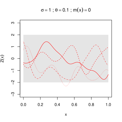
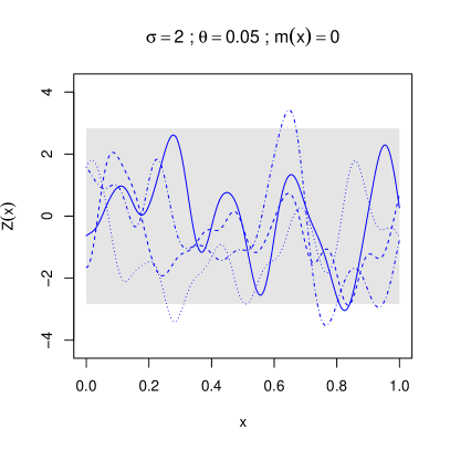
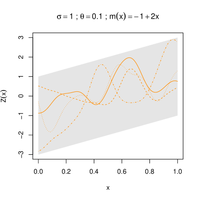
Figure 1: Examples of Gaussian process realizations with squared exponential kernels and different means. The shaded areas represent the point-wise 95% confidence intervals.

3.2 Gaussian process regression models

The principle of Gaussian process regression is to consider that the prior knowledge about the computational model $G(\boldsymbol{x})$, $\boldsymbol{x}\in\mathbb{R}^{d}$, can be modeled by a Gaussian process $Z(\boldsymbol{x})$ with a mean denoted by $m(\boldsymbol{x})$ and a covariance kernel denoted by $k(\boldsymbol{x},\boldsymbol{x}^{\prime})$. Roughly speaking, we consider that the true response is a realization of $Z(\boldsymbol{x})$. Usually, the mean and the covariance are parametrized as follows:

$$m(\boldsymbol{x})=\mathbf{f}^{\textsf{T}}(\boldsymbol{x})\boldsymbol{\beta},$$ (46)

and

$$k(\boldsymbol{x},\boldsymbol{x}^{\prime})=\sigma^{2}r(\boldsymbol{x},\boldsymbol{x}^{\prime};\boldsymbol{\theta}),$$ (47)

where $\mathbf{f}^{\textsf{T}}(\boldsymbol{x})$ is a vector of $p$ prescribed functions and $\boldsymbol{\beta}$, $\sigma^{2}$ and $\boldsymbol{\theta}$ have to be estimated. The mean function $m(\boldsymbol{x})$ describes the trend and the covariance kernel $k(\boldsymbol{x},\boldsymbol{x}^{\prime})$ describes the regularity and characteristic length scale of the model.

3.2.1 Predictive distribution

Consider an experimental design ${\mathcal{X}}=\left\{\boldsymbol{x}^{(1)},\dots,\boldsymbol{x}^{(n)}\right\}$, $\boldsymbol{x}^{(i)}\in\mathbb{R}^{d}$, and the corresponding model responses ${\mathcal{Y}}=G({\mathcal{X}})$. The predictive distribution of $G(\boldsymbol{x})$ is given by:

$$[Z(\boldsymbol{x})|Z({\mathcal{X}})={\mathcal{Y}},\sigma^{2},\boldsymbol{\theta}]\sim\mathrm{GP}\left(m_{n}(\boldsymbol{x}),k_{n}(\boldsymbol{x},\boldsymbol{x}^{\prime})\right),$$ (48)

where

$$m_{n}(\boldsymbol{x})=\mathbf{f}^{\textsf{T}}(\boldsymbol{x})\bar{\boldsymbol{\beta}}+\mathbf{r}^{\textsf{T}}(\boldsymbol{x})\mathbf{R}^{-1}\left({\mathcal{Y}}-\mathbf{F}\bar{\boldsymbol{\beta}}\right),$$ (49)

$$k_{n}(\boldsymbol{x},\boldsymbol{x}^{\prime})=\sigma^{2}\left(1-\begin{pmatrix}\mathbf{f}^{\textsf{T}}(\boldsymbol{x})&\mathbf{r}^{\textsf{T}}(\boldsymbol{x})\end{pmatrix}\begin{pmatrix}0&\mathbf{F}^{\textsf{T}}\\ \mathbf{F}&\mathbf{R}\end{pmatrix}\begin{pmatrix}\mathbf{f}(\boldsymbol{x}^{\prime})\\ \mathbf{r}(\boldsymbol{x}^{\prime})\end{pmatrix}\right),$$ (50)

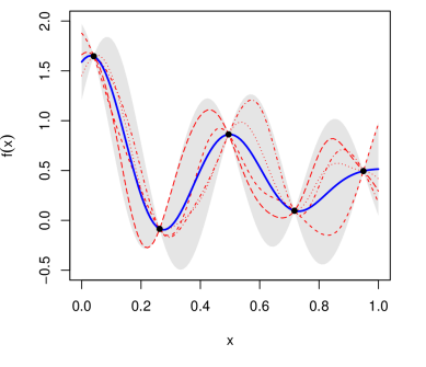
Figure 2: Examples of predictive distribution. The solid line represents the mean of the predictive distribution, the non-solid lines represent some of its realizations and the shaded area represents the 95% confidence intervals based on the variance of the predictive distribution.

In these expressions $\mathbf{R}=[r(\boldsymbol{x}^{i},\boldsymbol{x}^{j};\boldsymbol{\theta})]_{i,j=1,\dots,n}$, $\mathbf{r}(\boldsymbol{x})=[r(\boldsymbol{x},\boldsymbol{x}^{(i)};\boldsymbol{\theta})]_{i=1,\dots,n}$, $\mathbf{F}=[\mathbf{f}^{\textsf{T}}(\boldsymbol{x}^{(i)})]_{i=1,\dots,n}$ and

$$\bar{\boldsymbol{\beta}}=\left(\mathbf{F}^{\textsf{T}}\mathbf{R}^{-1}\mathbf{F}\right)^{-1}\mathbf{F}^{\textsf{T}}\mathbf{R}^{-1}{\mathcal{Y}}.$$ (51)

The term $\bar{\boldsymbol{\beta}}$ denotes the posterior distribution mode of $\boldsymbol{\beta}$ obtained from the improper non-informative prior distribution $\pi(\boldsymbol{\beta})\propto 1$ [44].

Remark. The predictive distribution is given by the Gaussian process $Z(x)$ conditioned by the known observations ${\mathcal{Y}}$. The Gaussian process regression metamodel is given by the conditional expectation $m_{n}(x)$ and its mean squared error is given by the conditional variance $k_{n}(\boldsymbol{x},\boldsymbol{x})$. An illustration of $m_{n}(x)$ and $k_{n}(\boldsymbol{x},\boldsymbol{x})$ is given in Figure 2.

The reader can note that the predictive distribution (48) integrates the posterior distribution of $\boldsymbol{\beta}$. However, the hyper-parameters $\sigma^{2}$ and $\boldsymbol{\theta}$ are not known in practice and shall be estimated with the maximum likelihood method [28; 46] or a cross-validation strategy [3]. Then, their estimates are plugged in the predictive distribution. The restricted maximum likelihood estimate of $\sigma^{2}$ is given by:

$$\hat{\sigma}^{2}=\frac{({\mathcal{Y}}-\mathbf{F}\bar{\boldsymbol{\beta}})^{\textsf{T}}\mathbf{R}^{-1}({\mathcal{Y}}-\mathbf{F}\bar{\boldsymbol{\beta}})}{n-p}.$$ (52)

Unfortunately, such a closed form expression does not exist for $\boldsymbol{\theta}$ and it has to be numerically estimated.

Remark. Gaussian process regression can easily be extended to the case of noisy observations. Let us suppose that ${\mathcal{Y}}$ is tainted by a white Gaussian noise $\varepsilon$ :

$${\mathcal{Y}}_{\mathrm{obs}}={\mathcal{Y}}+\sigma_{\varepsilon}(\boldsymbol{{\mathcal{X}}})\varepsilon.$$

The term $\sigma_{\varepsilon}(\boldsymbol{{\mathcal{X}}})$ represents the standard deviation of the observation noise. The mean and the covariance of the predictive distribution $[Z(\boldsymbol{x})_{\mathrm{obs}}|Z({\mathcal{X}})={\mathcal{Y}}_{\mathrm{obs}},\sigma^{2},\boldsymbol{\theta}]$ is then obtained by replacing in Equations (49), (50) and (51) the correlation matrix $\mathbf{R}$ by $\sigma^{2}\mathbf{R}+\mathbf{\Delta}_{\varepsilon}$ where $\mathbf{\Delta}_{\varepsilon}$ is a diagonal matrix given by :

$$\mathbf{\Delta}_{\varepsilon}=\begin{pmatrix}\sigma_{\varepsilon}(\boldsymbol{x}^{(1)})&&&\\ &\sigma_{\varepsilon}(\boldsymbol{x}^{(2)})&&\\ &&\ddots&\\ &&&\sigma_{\varepsilon}(\boldsymbol{x}^{(n)})\\ \end{pmatrix}.$$

We emphasize that the closed form expression for the restricted maximum likelihood estimate of $\sigma^{2}$ does not exist anymore. Therefore, this parameter has to be numerically estimated.

3.2.2 Sequential design

To improve the global accuracy of the GP model, it is usual to augment the initial design set ${\mathcal{X}}$ with new points. An important feature of Gaussian process regression is that it provides an estimate of the model mean-square error through the term $k_{n}(\boldsymbol{x},\boldsymbol{x}^{\prime})$ (50) which can be used to select these new points. The most common but not efficient sequential criterion consists in adding the point $\boldsymbol{x}^{(n+1)}$ where the mean-square error is the largest:

$$\boldsymbol{x}^{(n+1)}=\arg\max_{\boldsymbol{x}}k_{n}(\boldsymbol{x},\boldsymbol{x}).$$ (53)

More efficient criteria can be found in Bates et al. [4]; van Beers and Kleijnen [62]; Le Gratiet and Cannamela [33].

3.2.3 Model selection

To build up a GP model, the user has to make several choices. Indeed, the vector of functions $\mathbf{f}(\boldsymbol{x})$ and the class of the correlation kernel $r(\boldsymbol{x},\boldsymbol{x}^{\prime};\boldsymbol{\theta})$ need to be set (see Rasmussen and Williams [43] for different examples of correlation kernels). These choices and the relevance of the model are tested a posteriori with a validation procedure. If the number $n$ of observations is large, an external validation may be performed on a test set. Otherwise, a cross-validation procedure may be used. An interesting property of GP models is that a closed form expression exists for the cross-validation predictive distribution, see for instance Dubrule [23]. It allows for deriving efficient methods of parameter estimation [3] or sequential design [33].

Some usual stationary covariance kernel are listed below.

• The squared exponential covariance function. The form of this kernel is given by:

  $$k(\boldsymbol{x},\boldsymbol{x}^{\prime})=\sigma^{2}\mathrm{exp}\left(-\frac{1}{2\boldsymbol{\theta}^{2}}||\boldsymbol{x}-\boldsymbol{x}^{\prime}||^{2}\right).$$

  This covariance function corresponds to Gaussian processes which are infinitely differentiable in mean square and almost surely. We illustrate in Figure 3 the 1-dimensional squared exponential kernel with different correlation lengths and examples of resulting Gaussian process realizations.

  

  

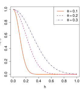
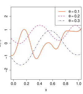
  Figure 3: The squared exponential kernel in function of $h=\boldsymbol{x}-\boldsymbol{x}^{\prime}$ with different correlation lengths $\boldsymbol{\theta}$ and examples of resulting Gaussian process realizations.

• The $\nu$-Matérn covariance function. This covariance kernel is defined as follow (see [54]):

  $$k_{\nu}(h)=\frac{2^{1-\nu}}{\Gamma(\nu)}\left(\frac{\sqrt{2}||h||}{\boldsymbol{\theta}}\right)^{\nu}K_{\nu}\left(\frac{\sqrt{2}\nu||h||}{\boldsymbol{\theta}}\right),$$

  where $\nu$ is the regularity parameter, $K_{\nu}$ is a modified Bessel Function and $\Gamma$ is the Euler Gamma function. A Gaussian process with a $\nu$-Matérn covariance kernel is $\nu$-Hölder continuous in mean square and $\nu^{\prime}$-Hölder continuous almost surely with $\nu^{\prime}<\nu$. Three popular choice of $\nu$-Matérn covariance kernels are the ones for $\nu=1/2$, $\nu=3/2$ and $\nu=5/2$ :

  $$k_{\nu=1/2}(h)=\exp\left(-\frac{||h||}{\boldsymbol{\theta}}\right),$$

  $$k_{\nu=3/2}(h)=\left(1+\frac{\sqrt{3}||h||}{\boldsymbol{\theta}}\right)\exp\left(-\frac{\sqrt{3}||h||}{\boldsymbol{\theta}}\right),$$

  and

  $$k_{\nu=5/2}(h)=\left(1+\frac{\sqrt{5}||h||}{\boldsymbol{\theta}}+\frac{{5}||h||^{2}}{3\boldsymbol{\theta}^{2}}\right)\exp\left(-\frac{\sqrt{5}||h||}{\boldsymbol{\theta}}\right).$$

  We illustrate in Figure 4 the 1-dimensional $\nu$-Matérn kernel for different values of $\nu$.

  

  

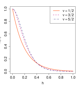
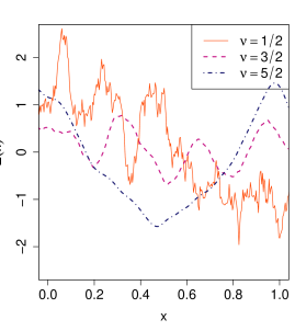
  Figure 4: The $\nu$-Matérn kernel in function of $h=\boldsymbol{x}-\boldsymbol{x}^{\prime}$ with different regularity parameters $\nu$ and examples of resulting Gaussian process realizations.

• The $\gamma$-exponential covariance function. This kernel is defined as follow:

  $$k_{\gamma}(h)=\exp\left(-\left(\frac{||h||}{\boldsymbol{\theta}}\right)^{\gamma}\right).$$

  For $\gamma<2$ the corresponding Gaussian process are not differentiable in mean square whereas for $\gamma=2$ is is infinitely differentiable (it corresponds to the squared exponential kernel). We illustrate in Figure 5 the 1-dimensional $\gamma$-exponential kernel for different values of $\gamma$.

  

  

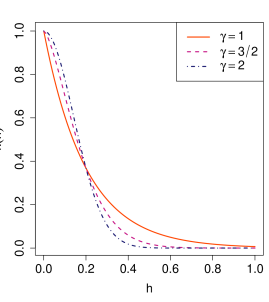
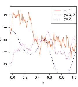
  Figure 5: The $\gamma$-exponetial kernel in function of $h=\boldsymbol{x}-\boldsymbol{x}^{\prime}$ with different regularity parameters $\gamma$ and examples of resulting Gaussian process realizations.

3.2.4 Sensitivity analysis

To perform a sensitivity analysis from a GP model, two approaches are possible. The first one consists in substituting the true model $G(\boldsymbol{x})$ with the mean of the conditional Gaussian process $m_{n}(\boldsymbol{x})$ in (49). However, it may provide biased sensitivity index estimates. Furthermore it does not allow one to quantify the error on the sensitivity indices due to the metamodel approximation. The second one consists in substituting $G(\boldsymbol{x})$ by a Gaussian process $Z_{n}(\boldsymbol{x})$ having the predictive distribution $[Z(\boldsymbol{x})|Z({\mathcal{X}})={\mathcal{Y}},\sigma^{2},\boldsymbol{\theta}]$ shown in (48). This approach makes it possible to quantify the uncertainty due to the metamodel approximation and allows for building unbiased index estimates.

3.3 Main effects visualization

From now on, the input parameter $\boldsymbol{x}\in\mathbb{R}^{d}$ is considered as a random input vector $\mathbf{X}=(X_{1},\dots,X_{d})$ with independent components. Before focusing on variance-based sensitivity indices, the inference about the main effects is studied in this section. Main effects are a powerful tool to visualize the impact of each input variable on the model output (see e.g. Oakley and O’Hagan [42]). The main effect of the group of input variables $\mathbf{X}_{A},\leavevmode\nobreak\ A\subset\left\{1,\dots,d\right\}$ is defined by $\mathbb{E}\left[G(\mathbf{X})|\mathbf{X}_{A}\right]$. Since the original model $G$ may be time-consuming to evaluate, it is substituted for by its approximation, i.e. $G(\boldsymbol{X})\approx\mathbb{E}\left[Z_{n}(\mathbf{X})|\mathbf{X}_{A}\right]$, where $Z_{n}(\boldsymbol{x})\sim[Z(\boldsymbol{x})|Z({\mathcal{X}})={\mathcal{Y}},\sigma^{2},\boldsymbol{\theta}]$. Since $\mathbb{E}\left[Z_{n}(\mathbf{X})|\mathbf{X}_{A}\right]$ is a linear transformation of the Gaussian process $Z_{n}(\boldsymbol{x})$, it is also a Gaussian process. The expectations, variances and covariances with respect to the posterior distribution of $[Z(\boldsymbol{x})|Z({\mathcal{X}})={\mathcal{Y}},\sigma^{2},\boldsymbol{\theta}]$ are denoted by $\mathbb{E}_{Z}\left[.\right]$, $\mathrm{Var}_{Z}\left(.\right)$ and $\mathrm{Cov}_{Z}\left(.,.\right)$. Then, we have:

$$\mathbb{E}\left[Z_{n}(\mathbf{X})|\mathbf{X}_{A}\right]\sim\mathrm{GP}\left(\mathbb{E}\left[m_{n}(\mathbf{X})|\mathbf{X}_{A}\right],\mathbb{E}\left[\mathbb{E}\left[k_{n}(\mathbf{X},\mathbf{X}^{\prime})|\mathbf{X}_{A}\right]|\mathbf{X}^{\prime}_{A}\right]\right).$$ (54)

The term $\mathbb{E}\left[m_{n}(\mathbf{X})\right]$ represents the approximation of $\mathbb{E}\left[G(\mathbf{X})|\mathbf{X}_{A}\right]$ and $\mathbb{E}\left[\mathbb{E}\left[k_{n}(\mathbf{X},\mathbf{X}^{\prime})|\mathbf{X}_{A}\right]|\mathbf{X}^{\prime}_{A}\right]$ is the mean-square error due to the metamodel approximation. Therefore, with this method one can quantify the error on the main effects due to the metamodel approximation. For more detail about this approach, the reader is referred to Oakley and O’Hagan [42]; Marrel et al. [37].

3.4 Variance of the main effects

Although the main effect enables one to visualize the impact of a group of variables on the model output, it does not quantify it. To perform such an analysis, consider the variance of the main effect:

$$V_{A}=\mathrm{Var}\left(\mathbb{E}\left[Z_{n}(\mathbf{X})|\mathbf{X}_{A}\right]\right),$$ (55)

or its normalized version which corresponds to the Sobol’ index:

$$S_{A}=\frac{V_{A}}{V}=\frac{\mathrm{Var}\left(\mathbb{E}\left[Z_{n}(\mathbf{X})|\mathbf{X}_{A}\right]\right)}{\mathrm{Var}\left(Z_{n}(\mathbf{X})\right)}.$$ (56)

Sobol’ indices are the most popular measures to carry out a sensitivity analysis since their value can easily be interpreted as the part of the total variance due to a group of variables. However, in contrary to the partial variance $V_{A}$, it does not provide information about the order of magnitude of the contribution to the model output variance of variable group $\mathbf{X}_{A}$.

3.4.1 Analytic formulae

The above indices are studied in Oakley and O’Hagan [42] where the estimation of $V_{A}$ and $V$ is performed separately. Indeed, computing the Sobol’ index $S_{A}$ requires considering the joint distribution of $V_{A}$ and $V$, which makes it impossible to derive analytic formulae. According to Oakley and O’Hagan [42], closed form expressions in terms of integrals can be obtained for the two quantities $\mathbb{E}_{Z}\left[V_{A}\right]$ and $\mathrm{Var}_{Z}\left(V_{A}\right)$. The quantity $\mathbb{E}_{Z}\left[V_{A}\right]$ is the sensitivity measure and $\mathrm{Var}_{Z}\left(V_{A}\right)$ represents the error due to the metamodel approximation. Nevertheless, $V_{A}$ is not a linear transform of $Z_{n}(\mathbf{X})$ and its full distribution cannot be established.

3.4.2 Variance estimates with Monte-Carlo integration

To evaluate the Sobol’ index $S_{A}$, it is possible to use the pick-freeze approaches presented in Chapter 4 and in Sobol [50]; Sobol et al. [52]; Janon et al. [31]. By considering the formula given in Sobol [50], $S_{A}$ can be approximated by:

$$S_{A,N}=\frac{\frac{1}{N}\sum_{i=1}^{N}Z_{n}(\mathbf{X}^{(i)})Z_{n}(X_{\leavevmode\nobreak\ A}^{(i)})-\left(\frac{1}{2N}\sum_{i=1}^{N}Z_{n}(\mathbf{X}^{(i)})+Z_{n}(X_{\leavevmode\nobreak\ A}^{(i)})\right)^{2}}{\frac{1}{N}\sum_{i=1}^{N}Z_{n}(\mathbf{X}^{(i)})^{2}-\left(\frac{1}{2N}\sum_{i=1}^{N}Z_{n}(\mathbf{X}^{(i)})+Z_{n}(X_{\leavevmode\nobreak\ A}^{(i)})\right)^{2}},$$ (57)

where $(\mathbf{X}^{(i)},X_{\leavevmode\nobreak\ A}^{(i)})_{i=1,\dots,N}$ is a $N$-sample from the random variable $(\mathbf{X},\mathbf{X}^{\sim A})$.

In particular, this approach avoids to compute the integrals presented in Oakley and O’Hagan [42] and thus simplify the estimation of $V_{A}$ and $V$. Furthermore, it takes into account their joint distribution.

Remark.

This result can easily be extended to the total Sobol’ index $S^{\mbox{\scriptsize{tot}}}_{i}=\sum\limits_{A\supset\,i}S_{A}$. The reader is referred to Sobol et al. [52] and Variance-based sensitivity analysis: Theory and estimation algorithms in this handbook for examples of pick-freeze estimates of $S_{A}^{\mbox{\scriptsize{tot}}}$.

3.5 Numerical estimates of Sobol’ indices by Gaussian process sampling

The sensitivity index $S_{A,N}$ (57) is obtained after substituting the Gaussian process $Z_{n}(\boldsymbol{x})$ for the original computational model $G(\boldsymbol{x})$. Therefore, it is a random variable defined on the same probability space as $Z_{n}(\boldsymbol{x})$. The aim of this section is to present a simple methodology to get a sample $S_{A,N}$ of $S_{A}$. From this sample, an estimate of $S_{A}$ (56) and a quantification of its uncertainty can be deduced.

Sampling from the Gaussian predictive distribution

To obtain a realization of $S_{A,N}$, one has to obtain a sample of $Z_{n}(\boldsymbol{x})$ on $(\mathbf{X}^{(i)},X_{\leavevmode\nobreak\ A}^{(i)})_{i=1,\dots,N}$ and then use Eq. (57). To deal with large $N$, an efficient strategy is to sample $Z_{n}(\boldsymbol{x})$ using the Kriging conditioning method, see for example Chilès and Delfiner [18]. Consider first the unconditioned, zero-mean Gaussian process:

$$\tilde{Z}(\boldsymbol{x})=\mathrm{GP}\left(0,k(\boldsymbol{x},\boldsymbol{x}^{\prime})\right).$$ (58)

Then, the Gaussian process:

$$\tilde{Z}_{n}(\boldsymbol{x})=m_{n}(\boldsymbol{x})-\tilde{m}_{n}(\boldsymbol{x})+\tilde{Z}(\boldsymbol{x}),$$ (59)

where $\tilde{m}_{n}(\boldsymbol{x})=\mathbf{f}^{\textsf{T}}(\boldsymbol{x})\tilde{\boldsymbol{\beta}}+\mathbf{r}^{\textsf{T}}(\boldsymbol{x})\mathbf{R}^{-1}\left(\tilde{Z}({\mathcal{X}})-\mathbf{F}\tilde{\boldsymbol{\beta}}\right)$ and $\tilde{\boldsymbol{\beta}}=\left(\mathbf{F}^{\textsf{T}}\mathbf{R}^{-1}\mathbf{F}\right)^{-1}\mathbf{F}^{\textsf{T}}\mathbf{R}^{-1}\tilde{Z}({\mathcal{X}})$ has the same distribution as $Z_{n}(\boldsymbol{x})$. Therefore, one can compute realizations of $Z_{n}(\boldsymbol{x})$ from realizations of $\tilde{Z}(\boldsymbol{x})$. Since $\tilde{Z}(\boldsymbol{x})$ is not conditioned, the problem is numerically easier. Among the available Gaussian process sampling methods, several can be mentioned: Cholesky decomposition [43], Fourier spectral decomposition [54], Karhunen-Loeve spectral decomposition [43] and the propagative version of the Gibbs sampler [32].

Remark.

Let suppose that a new point $\boldsymbol{x}^{(n+1)}$ is added to the experimental design ${\mathcal{X}}$. A classical result of conditional probability implies that the new predictive distribution $[Z(\boldsymbol{x})|Z({\mathcal{X}})={\mathcal{Y}},Z(\boldsymbol{x}^{(n+1)})=G(\boldsymbol{x}^{(n+1)}),\sigma^{2},\boldsymbol{\theta}]$ is identical to $[Z_{n}(\boldsymbol{x})|Z_{n}(\boldsymbol{x}^{(n+1)})=G(\boldsymbol{x}^{(n+1)}),\sigma^{2},\boldsymbol{\theta}]$. Therefore, $Z_{n}(\boldsymbol{x})$ can be viewed as an unconditioned Gaussian process and, using the Kriging conditioning method, realizations of $[Z(\boldsymbol{x})|Z({\mathcal{X}})={\mathcal{Y}},Z(\boldsymbol{x}^{(n+1)})=G(\boldsymbol{x}^{(n+1)}),\sigma^{2},\boldsymbol{\theta}]$ can be derived from realizations of $Z_{n}(\boldsymbol{x})$ using the following equation:

$$Z_{n+1}(\boldsymbol{x})=\frac{k_{n}(\boldsymbol{x}^{(n+1)},{\mathcal{X}})}{k_{n}(\boldsymbol{x}^{(n+1)},\boldsymbol{x}^{(n+1)})}\left(G(\boldsymbol{x}^{(n+1)})-Z_{n}(\boldsymbol{x}^{(n+1)})\right)+Z_{n}(\boldsymbol{x}).$$ (60)

Therefore, it is easy to calculate a new sample of $S_{A,N}$ after adding a new point $\boldsymbol{x}^{(n+1)}$ to the experimental design set ${\mathcal{X}}$. This result is used in the R CRAN package “sensitivity” to perform sequential design for sensitivity analysis using a Stepwise Uncertainty Reduction (SUR) strategy [5].

3.5.1 Meta-model and Monte-Carlo sampling errors

Let us denote by $\left\{S_{A,i}^{N},\leavevmode\nobreak\ i=1,\dots,m\right\}$ a sample set of $S_{A,N}$ (57) where of size $m>0$. From this sample set, the following unbiased estimate of $S_{A}$ can be deduced:

$$\hat{S}_{A}=\frac{1}{m}\sum_{i=1}^{m}S_{A,i}^{N}.$$ (61)

with variance:

$$\hat{\sigma}_{\hat{S}_{A}}^{2}=\frac{1}{m-1}\sum_{i=1}^{m}\left(S_{A,i}^{N}-\hat{S}_{A}\right)^{2}.$$ (62)

The term $\hat{\sigma}_{\hat{S}_{A}}^{2}$ represents the uncertainty on the estimate of $S_{A}$ (56) due to the metamodel approximation. Therefore, with the presented strategy, one can both obtain an unbiased estimate of the sensitivity index $S_{A}$ and a quantification of its uncertainty.

Finally it may be of interest to evaluate the error due to the pick-freeze approximation and to compare it to the error due to the metamodel. To do so, one can use the central limit theorem [31; 17] or a bootstrap procedure [34]. In particular, a methodology to evaluate the uncertainty on the sensitivity index due to both the Gaussian process and to the pick-freeze approximations is presented in Le Gratiet et al. [34]. It makes it possible to determine the value of $N$ such that the pick-freeze approximation error is negligible compared to that of the metamodel.

3.6 Summary

Gaussian Process regression makes it possible to perform sensitivity analysis on complex computational models using a limited number of model evaluations. An important feature of this method is that one can propagate the Gaussian process approximation error to the sensitivity index estimates. This allows the construction of sequential design strategies optimized for sensitivity analysis. It also provides a powerful tool to visualize the main effect of a group of variables and the uncertainty of its estimate. Another advantage of this approach is that Gaussian process regression has been thoroughly investigated in the literature and can be used in various problems. For example, the method can be adapted for non-stationary numerical models by using a treed Gaussian process as in Gramacy and Taddy [27]. Furthermore, it can also be used for multifidelity computer codes, i.e. codes which can be run at multiple level of accuracy (see Le Gratiet et al. [34]).

4 Applications

In this section, metamodel-based sensitivity analysis is illustrated on several academic and engineering examples.

4.1 Ishigami function

The Ishigami function is given by:

$$G(x_{1},x_{2},x_{3})=\sin(x_{1})+7\sin(x_{2})^{2}+0.1x_{3}^{4}\sin(x_{1}).$$ (63)

The input distributions of $X_{1},X_{2}$ and $X_{3}$ are uniform over the interval $[-\pi,\pi]^{3}$. This is a classical academic benchmark for sensitivity analysis, with first-order Sobol’ indices:

$$S_{1}=0.3138\qquad S_{2}=0.4424\qquad S_{3}=0.$$ (64)

To compare polynomial chaos expansions and Gaussian process modeling on this example, experimental designs of different sizes $n$ are considered. For each size $n$, 100 Latin Hypercube Sampling sets (LHS) are computed so as to replicate the procedure and assess statistical uncertainty.

For the polynomial chaos approach, the coefficients are calculated based on a degree-adaptive LARS strategy (for details, see Blatman and Sudret [13]), resulting in a sparse basis set. The maximum polynomial degree is adaptively selected in the interval $3\leq p\leq 15$ based on LOO cross-validation error estimates (see Eq. (27)).

For the Gaussian process approach, a tensorized Matérn-$5/2$ covariance kernel is chosen (see Rasmussen and Williams [43]) with trend functions given by:

$$\mathbf{f}^{\textsf{T}}(\boldsymbol{x})=\left\{1\leavevmode\nobreak\ \leavevmode\nobreak\ x_{2}\leavevmode\nobreak\ \leavevmode\nobreak\ x_{2}^{2}\leavevmode\nobreak\ \leavevmode\nobreak\ x_{1}^{3}\leavevmode\nobreak\ \leavevmode\nobreak\ x_{2}^{3}\leavevmode\nobreak\ \leavevmode\nobreak\ x_{1}^{4}\leavevmode\nobreak\ \leavevmode\nobreak\ x_{2}^{4}\right\}.$$ (65)

The hyper-parameters $\boldsymbol{\theta}$ are estimated with a Leave-One-Out cross validation procedure while the parameters $\boldsymbol{\beta}$ and $\sigma^{2}$ are estimated with a restricted maximum likelihood method.

First we illustrate in Figure 6 the accuracy of the models with respect to the sample size $n$. The Nash-Sutcliffe model efficiency coefficient (also called predictivity coefficient) is defined as follows:

$$Q^{2}=1-\frac{\sum_{i=1}^{n_{\mathrm{test}}}(G(\boldsymbol{x}^{(i)})-\hat{G}(\boldsymbol{x}^{(i)}))^{2}}{\sum_{i=1}^{n_{\mathrm{test}}}(G(\boldsymbol{x}^{(i)})-\bar{G})^{2}},\quad\bar{G}=\frac{1}{{n_{\mathrm{test}}}}\sum_{i=1}^{n_{\mathrm{test}}}G(\boldsymbol{x}^{(i)}),$$ (66)

where $\hat{G}(\boldsymbol{x}^{(i)})$ is the prediction given by the polynomial chaos or the Gaussian process regression model on the $i^{\mathrm{th}}$ point of a test sample of size ${n_{\mathrm{test}}}=10,000$. This test sample set is randomly generated from a uniform distribution. The closer $Q^{2}$ is to 1, the more accurate the metamodel is.

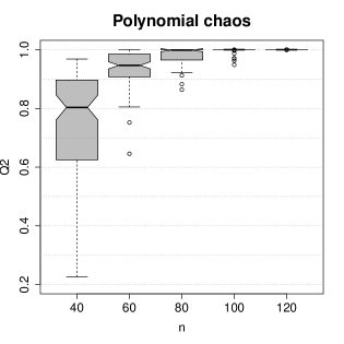
Figure 6: $Q^{2}$ coefficient as a function of the sample size $n$ for the Ishigami function. For each $n$, the box-plots represent the variations of $Q^{2}$ obtained over 100 LHS replications.

We emphasize that checking the metamodel accuracy (see Figure 6) is very important since a metamodel-based sensitivity analysis provides sensitivity indices for the metamodel and not for the true model $G(\boldsymbol{x})$. Therefore, the estimated indices are relevant only if the considered surrogate model is accurate.

Figure 7 shows the Sobol’ index estimates with respect to the sample size $n$. For the Gaussian process regression approach, the convergence for is reached for $n=100$. It corresponds to a $Q^{2}$ coefficient greater than 90%. Convergence of the PCE approach is somewhat faster, with comparable accuracy achieved with $n=60$ and almost perfect accuracy for $n=100$. Therefore, the convergence of the estimators of the Sobol’ indices in Eqs. (36) to (39) is expected to be comparable to that of $Q^{2}$. Note that the PCE approach also provides second order- and total Sobol’ indices for free, as shown in Sudret [59].

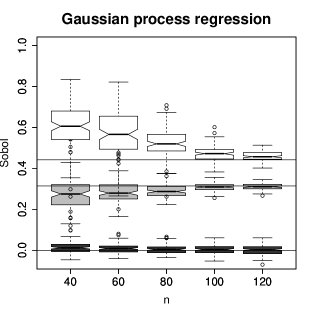
Figure 7: First-order Sobol’ index estimates as a function of the sample size $n$ for the Ishigami function. The horizontal solid lines represent the exact values of $S_{1}$, $S_{2}$ and $S_{3}$. For each $n$, the box-plot represents the variations obtained from 100 LHS replications. The validation set comprises $n_{test}=10,000$ samples.

4.2 G-Sobol function

The G-Sobol function is given by :

$$G(\boldsymbol{x})=\prod_{i=1}^{d}\frac{|4x_{i}-2|+a_{i}}{1+a_{i}},\quad a_{i}\geq 0.$$ (67)

To benchmark the described metamodel-based sensitivity analysis methods in higher dimension, we select $d=15$. The exact first-order Sobol’ indices $S_{i}$ are given by the following equations:

$$\begin{split}V_{i}&=\frac{1}{3(1+a_{i})^{2}},\quad i=1,\dots,d,\\ V&=\prod_{i=1}^{d}(1+V_{i})-1,\\ S_{i}&=V_{i}/V.\end{split}$$ (68)

In this example, vector $\boldsymbol{a}=\left\{a_{1},a_{2},\dots,a_{d}\right\}$ is equal to:

$$\boldsymbol{a}=\left\{1,2,5,10,20,50,100,500,1000,1000,1000,1000,1000,1000,1000\right\}.$$ (69)

As in the previous section, different sample sizes $n$ are considered and 100 LHS replications are computed for each $n$. Sparse polynomial chaos expansions are obtained with the same strategy as for the Ishigami function: adaptive polynomial degree selection with $3<p<15$ and LARS-based calculation of the coefficients. For the Gaussian process regression model, a tensorized Matérn-5/2 covariance kernel is considered with a constant trend function $\mathbf{f}(\boldsymbol{x})=1$. The hyper-parameter $\boldsymbol{\theta}$ is estimated with a Leave-One-Out cross validation procedure and the parameters $\boldsymbol{\beta}$ and $\sigma^{2}$ are estimated with the maximum likelihood method.

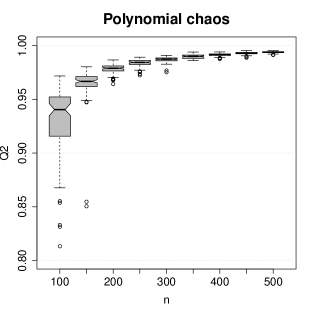
Figure 8: $Q^{2}$ coefficient as a function of the sample size $n$ for G-Sobol academic example. For each $n$, the box-plot represents the variations of $Q^{2}$ obtained from 100 LHS.

The accuracy of the metamodels with respect to $n$ is presented in Figure 8. It is computed from a test sample set of size $n_{\mathrm{test}}=10,000$. The convergence of the estimates of the first four first-order Sobol’ indices is represented in Figure 9. Both metamodel-based estimations yield excellent results already with $n=100$ samples in the experimental design. This is expected due to the good accuracy of both metamodels for all the $n$ considered (see Figure 8).

Figure 9: Sobol’ index estimates with respect to the sample size $n$ for G-Sobol function. The horizontal solid lines represent the true values of $S_{1}$, $S_{2}$, $S_{3}$ and $S_{4}$. For each $n$, the box-plot represents the variations obtained from 100 LHS.

Finally, Table 2 provides the Sobol’ index estimates median and root mean square error for $n=100$ and $n=500$. As presented in Figure 9, the estimates of the largest Sobol’ indices are very accurate. Note that the remaining first order indices are insignificant. One can observe that the RMS error over the 100 LHS replications is slightly smaller when using PCE for both $n=100$ and $n=500$ ED points. Note that the second order- and total Sobol’ indices are also available for free when using PCE.

Table 2: Sobol’ index estimates for the G-Sobol function. The median and the root mean square error (RMSE) of the estimates are given for $n=100$ and $n=500$.

		Polynomial chaos expansion				Gaussian process regression
		Median		RMSE		Median		RMSE
Index	Value	100	500	100	500	100	500	100	500
$S_{1}$	0.604	0.619	0.607	0.034	0.007	0.618	0.599	0.035	0.012
$S_{2}$	0.268	0.270	0.269	0.027	0.005	0.233	0.245	0.046	0.026
$S_{3}$	0.067	0.063	0.065	0.014	0.003	0.045	0.070	0.029	0.016
$S_{4}$	0.020	0.014	0.019	0.008	0.001	0.008	0.023	0.018	0.013
$S_{5}$	0.005	0.002	0.005	0.003	0.001	8.6$\times 10^{-4}$	1.8$\times 10^{-3}$	0.014	0.013
$S_{6}$	0.001	0.000	7.2$\times 10^{-4}$	0.001	3.5$\times 10^{-4}$	6.4$\times 10^{-4}$	5.3$\times 10^{-4}$	0.013	0.013
$S_{7}$	0.000	0.000	1.1$\times 10^{-4}$	1.1$\times 10^{-3}$	1.4$\times 10^{-4}$	5.3$\times 10^{-4}$	3.0$\times 10^{-4}$	0.013	0.013
$S_{8}$	0.000	0.000	0.000	3.3$\times 10^{-4}$	1.7$\times 10^{-5}$	6.5$\times 10^{-4}$	7.1$\times 10^{-4}$	0.013	0.013
$S_{9}$	0.000	0.000	0.000	4.1$\times 10^{-4}$	1.1$\times 10^{-5}$	8.5$\times 10^{-4}$	4.4$\times 10^{-4}$	0.14	0.013
$S_{10}$	0.000	0.000	0.000	2.4$\times 10^{-4}$	1.1$\times 10^{-5}$	2.2$\times 10^{-4}$	1.7$\times 10^{-4}$	0.013	0.013
$S_{11}$	0.000	0.000	0.000	9.5 $\times 10^{-4}$	1.2$\times 10^{-5}$	5.5$\times 10^{-4}$	-9.9$\times 10^{-5}$	0.013	0.013
$S_{12}$	0.000	0.000	0.000	5.2$\times 10^{-4}$	2.1 $\times 10^{-5}$	2.6$\times 10^{-4}$	4.1$\times 10^{-4}$	0.013	0.013
$S_{13}$	0.000	0.000	0.000	5.1$\times 10^{-4}$	5.9 $\times 10^{-6}$	9.8$\times 10^{-4}$	4.7$\times 10^{-4}$	0.013	0.013
$S_{14}$	0.000	0.000	0.000	8.8$\times 10^{-4}$	1.9 $\times 10^{-5}$	1.8$\times 10^{-4}$	6.9$\times 10^{-4}$	0.013	0.013
$S_{15}$	0.000	0.000	0.000	8.6$\times 10^{-4}$	9.7$\times 10^{-6}$	7.2$\times 10^{-4}$	3.1$\times 10^{-4}$	0.013	0.013

4.3 Morris function

The Morris function is given by [49]:

$$G(\boldsymbol{x})=\sum_{i=1}^{20}\beta_{i}w_{i}+\sum_{i<j}^{20}\beta_{ij}w_{i}w_{j}+\sum_{i<j<l}^{20}\beta_{ijl}w_{i}w_{j}w_{l}+5w_{1}w_{2}w_{3}w_{4}$$ (70)

where $X_{i}\sim{\mathcal{U}}(0,1),\,i=1,\ldots,20$ and $w_{i}=2(x_{i}-1/2)$ for all $i$ except for $i=3,5,7$ where $w_{i}=2(1.1x_{i}/(x_{i}+0.1)-1/2)$. The coefficients are defined as $\beta_{i}=20,\,i=1,\ldots,10$; $\beta_{ij}=-15,\,i,j=1,\ldots,6$; $\beta_{ijl}=-10,\,i,j,l=1,\ldots,5$. The remaining coefficients are set equal to $\beta_{i}=(-1)^{i}$ and $\beta_{ij}=(-1)^{i+j}$ and all the rest are zero. The reference values of the first-order Sobol’ indices of the Morris function are calculated by a large Monte Carlo-based sensitivity analysis ($n=10^{6}$).

As in the previous section different sample sizes $n$ are considered and 100 LHS replications are computed for each $n$. Sparse polynomial chaos expansions are obtained by adaptive polynomial degree selection $5<p<13$ and LARS-based calculation of the coefficients.

Figure 10: $Q^{2}$ coefficient as a function of the sample size $n$ for the Morris function example. For each $n$, the box-plot represents the variations of $Q^{2}$ obtained from 100 LHS.

The accuracy of the metamodels with respect to $n$ is presented in Figure 10. It is computed from a test sample of size $n_{test}=10,000$. As expected due to the complexity and dimensionality of the Morris function, both metamodels show a slower overall convergence rate with the number of samples with respect to the previous examples. Polynomial chaos expansions show in this case remarkably more scattering in their performance for smaller experimental designs with respect to Gaussian process regression. This is likely due to the comparatively large amount of prior information in the form of trend functions provided to the Gaussian process, not used for PCE.

The convergence of the estimates of three selected first-order Sobol’ indices (the largest $S_{9}$ and two intermediate ones $S_{3}$ and $S_{8}$) is represented in Figure 11. Both methods perform very well with as few as 250 samples. PCE, however, shows a more standard convergence behavior both in mean value in dispersion. Gaussian process regression retrieves the Sobol’ estimates very accurately even with extremely small experimental designs, but no clear convergence pattern can be seen for larger datasets.

Finally, Table 3 provides the a detailed breakdown of the Sobol’ index estimates, including median and root mean square error (RMSE), for $n=100$ and $n=500$.

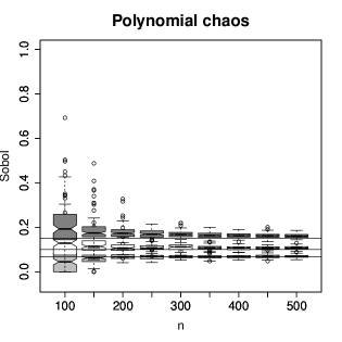
Figure 11: First-order Sobol’ index estimates as a function of the sample size $n$ for the Morris function. The horizontal solid lines represent the exact values of $S_{3}$, $S_{8}$ and $S_{9}$. For each $n$, the box-plot represents the variations obtained from 100 LHS replications.

Table 3: First-order Sobol’ indices estimation for the Morris function. The median and the root mean square error (RMSE) of the estimates are given for $n=100$ and $n=500$.

		Polynomial chaos expansion				Gaussian process regression
		Median		RMSE		Median		RMSE
Index	Value	100	500	100	500	100	500	100	500
$S_{2}$	0.005	0.000	0.005	0.252	0.017	0.011	0.004	0.109	0.085
$S_{3}$	0.008	0.000	0.009	0.175	0.027	0.006	0.007	0.089	0.088
$S_{1}$	0.017	0.000	0.015	0.304	0.047	0.003	0.017	0.130	0.109
$S_{4}$	0.009	0.000	0.009	0.119	0.023	0.017	0.011	0.130	0.097
$S_{5}$	0.016	0.000	0.015	0.230	0.043	0.005	0.016	0.120	0.109
$S_{6}$	0.000	0.000	0.000	0.061	0.003	0.000	0.000	0.061	0.070
$S_{7}$	0.069	0.045	0.068	0.585	0.058	0.072	0.062	0.095	0.123
$S_{8}$	0.100	0.128	0.107	0.950	0.105	0.105	0.116	0.108	0.211
$S_{9}$	0.150	0.192	0.160	1.241	0.143	0.127	0.143	0.246	0.117
$S_{10}$	0.100	0.133	0.106	0.875	0.092	0.138	0.111	0.404	0.155
$S_{11}$	0.000	0.000	0.000	0.185	0.003	0.004	0.000	0.088	0.074
$S_{12}$	0.000	0.000	0.000	0.083	0.004	0.000	0.000	0.064	0.077
$S_{13}$	0.000	0.000	0.000	0.081	0.003	0.000	0.000	0.064	0.074
$S_{14}$	0.000	0.000	0.000	0.020	0.003	0.000	0.000	0.070	0.078
$S_{15}$	0.000	0.000	0.000	0.140	0.003	0.000	0.000	0.065	0.075
$S_{16}$	0.000	0.000	0.000	0.040	0.005	0.001	0.000	0.077	0.074
$S_{17}$	0.000	0.000	0.000	0.264	0.004	0.000	0.000	0.065	0.075
$S_{18}$	0.000	0.000	0.000	0.084	0.004	0.000	0.000	0.064	0.075
$S_{19}$	0.000	0.000	0.000	0.083	0.004	0.000	0.000	0.064	0.076
$S_{20}$	0.000	0.000	0.000	0.049	0.004	0.000	0.000	0.064	0.075

4.4 Maximum deflection of a truss structure

Sensitivity analysis is also of great interest for engineering models whose input parameters may have different distributions. As an example consider the elastic truss structure depicted in Figure 12 (see e.g. Blatman and Sudret [10]). This truss is made of two types of bars, namely horizontal bars with cross-section $A_{1}$ and Young’s modulus (stiffness) $E_{1}$ on the one hand oblique bars with cross-section $A_{2}$ and Young’s modulus (stiffness) $E_{2}$ on the other hand. The truss is loaded with six vertical loads applied on the top chord. Of interest is the maximum vertical displacement (called deflection) at mid-span. This quantity is computed using a finite element model comprising elastic bar elements.

Figure 12: Model of a truss structure with 23 members. The quantity of interest is the maximum displacement at mid-span $u_{4}$.

The various parameters describing the behavior of this truss structure are modeled by independent random variables that account for the uncertainty in both the physical properties of the structure and the applied loads. Their distributions are gathered in Table 4.

Table 4: Probabilistic input model of the truss structure

Variable	Distribution	Mean	Standard Deviation
$E_{1}$, $E_{2}$ (Pa)	Lognormal	$2.1\times 10^{11}$	$2.1\times 10^{10}$
$A_{1}$ (m2)	Lognormal	$2.0\times 10^{-3}$	$2.0\times 10^{-4}$
$A_{2}$ (m2)	Lognormal	$1.0\times 10^{-3}$	$1.0\times 10^{-4}$
$P_{1}$-$P_{6}$ (N)	Gumbel	$5.0\times 10^{4}$	$7.5\times 10^{3}$

These input variables are collected in the random vector

$$\boldsymbol{X}=\left\{E_{1},E_{2},A_{1},A_{2},P_{1},\dots,P_{6}\right\}.$$ (71)

Using this notation, the maximal deflection of interest is cast as:

$$u_{4}=G^{\text{FE}}(\boldsymbol{X}).$$ (72)

Different sparse polynomial chaos expansions are calculated assuming a maximal degree $3<p<10$ using LARS and the best expansion (in terms of smallest LOO error) is retained. For the Gaussian process regression model, a tensorized Matérn-5/2 covariance kernel is considered with a constant trend function $\mathbf{f}(\boldsymbol{x})=1$. The hyper-parameter $\boldsymbol{\theta}$ is estimated with a Leave-One-Out cross validation procedure and the parameters $\boldsymbol{\beta}$ and $\sigma^{2}$ are estimated with the maximum likelihood method.

The first order Sobol’ indices obtained from PCE and GP metamodels are reported in Table 5 in the case when the experimental design is of size 100. In decreasing importance order, the important variables are the properties of the chords (horizontal bars), then the loads close to mid-span, namely $P_{3}$ and $P_{4}$. The Sobol’ indices of the latter are identical due to the symmetry of the model. Then come the loads $P_{2}$ and $P_{5}$. The other variables (the loads $P_{1}$ and $P_{6}$ and the properties of the oblique bars) appear unimportant.

Table 5: Truss structure – First order Sobol’ indices

Variable	Reference	PCE	Gaussian Process
$A_{1}$	0.365	0.366	0.384
$E_{1}$	0.365	0.369	0.362
$P_{3}$	0.075	0.078	0.075
$P_{4}$	0.074	0.076	0.069
$P_{5}$	0.035	0.036	0.029
$P_{2}$	0.035	0.036	0.028
$A_{2}$	0.011	0.012	0.015
$E_{2}$	0.011	0.012	0.008
$P_{6}$	0.003	0.005	0.002
$P_{1}$	0.002	0.005	0.000

The estimates of the three largest first-order Sobol’ indices which correspond to variables $E_{1}$, $P_{3}$ and $P_{5}$ obtained for various sizes $n$ of the LHS experimental design are plotted in Figure 13 as a function of $n$. The reference solution is obtained by Monte-Carlo sampling with a sample set of size 6,000,000. Both PCE- and GP-based Sobol’ indices converge to stable estimates as soon as $n\geq 60$.

Figure 13: Truss structure – First-order Sobol’ index estimates as a function of the sample size $n$ for the truss model. The horizontal solid lines represent reference values of input variables $E_{1}$, $P_{3}$ and $P_{5}$ from a Monte Carlo estimate on 6,000,000 samples.

5 Conclusions

Sobol’ indices are recognized as good descriptors of the sensitivity of the output of a computational model to its various input parameters. Classical estimation methods based on Monte Carlo simulation are computationally expensive though. The required costs, in the order of $10^{3}-10^{4}$ model evaluations, are often not compatible with the advanced simulation models encountered in engineering applications.

For this reason, surrogate models may be first built up from a limited number of runs of the computational model (the so-called experimental design), and the sensitivity analysis is then carried out by substituting the surrogate model for the original one.

Polynomial chaos expansions and Gaussian processes are two popular methods that can be used for this purpose. The advantage of the PCE approach is that the Sobol’ indices at any order may be computed analytically once the expansion is available. In this contribution, least-square minimization techniques are presented to compute the PCE coefficients, yet any intrusive or non intrusive method could be used as an alternative.

In contrast Gaussian process surrogate models are used together with Monte Carlo simulation for estimating the Sobol’ indices. The advantage of this approach is that the metamodel error can be included in the estimators. Note that bootstrap techniques can be used similarly to calculate and include metamodeling error also for PCE-based sensitivity analysis, as demonstrated by Dubreuil et al. [22].

As shown in the various comparisons, PCE and GP give similar accuracy (measured in terms of the $Q^{2}$ validation coefficient) for a given size of the experimental design in a broad range of applications. The replication of the analyses with different random designs of the same size show a smaller scatter using GP for extremely small designs, whereas PCE becomes more stable for medium-size designs. Selecting the best technique is in the end problem-dependent, and it is worth comparing the two approaches using the same experimental design, as it can be done in recent sensitivity analysis toolboxes such as OpenTURNS [2] and UQLab [36].

Finally it is worth mentioning that the so-called derivative-based global sensitivity measures (DGSM) originally introduced by Sobol’ and Kucherenko [51] can also be computed using surrogate models. In particular, polynomial chaos expansions may be used to compute the DGSM analytically, as shown in Sudret and Mai [61]. The recent combination of polynomial chaos expansions and Gaussian processes into PC-Kriging [48] also appears promising for estimating sensitivity indices from extremely small experimental designs.

References

- Abramowitz and Stegun (1970) Abramowitz, M. and I. Stegun (1970). Handbook of mathematical functions. Dover Publications, Inc.
- Andrianov et al. (2007) Andrianov, G., S. Burriel, S. Cambier, A. Dutfoy, I. Dutka-Malen, E. de Rocquigny, B. Sudret, P. Benjamin, R. Lebrun, F. Mangeant, and M. Pendola (2007). Open TURNS, an open source initiative to Treat Uncertainties, Risks’N Statistics in a structured industrial approach. In Proc. ESREL’2007 Safety and Reliability Conference, Stavenger, Norway.
- Bachoc (2013) Bachoc, F. (2013). Cross validation and maximum likelihood estimations of hyper-parameters of gaussian processes with model misspecification. Computational Statistics & Data Analysis 66, 55–69.
- Bates et al. (1996) Bates, R. A., R. Buck, E. Riccomagno, and H. Wynn (1996). Experimental design and observation for large systems. Journal of the Royal Statistical Society, Series B 58 (1), 77–94.
- Bect et al. (2012) Bect, J., D. Ginsbourger, L. Li, V. Picheny, and E. Vazquez (2012). Sequential design of computer experiments for the estimation of a probability of failure. Statistics and Computing 22, 773–793.
- Berveiller et al. (2004) Berveiller, M., B. Sudret, and M. Lemaire (2004). Presentation of two methods for computing the response coefficients in stochastic finite element analysis. In Proc. 9th ASCE Specialty Conference on Probabilistic Mechanics and Structural Reliability, Albuquerque, USA.
- Berveiller et al. (2006) Berveiller, M., B. Sudret, and M. Lemaire (2006). Stochastic finite elements: a non intrusive approach by regression. Eur. J. Comput. Mech. 15(1-3), 81–92.
- Bieri and Schwab (2009) Bieri, M. and C. Schwab (2009). Sparse high order FEM for elliptic sPDEs. Comput. Methods Appl. Mech. Engrg 198, 1149–1170.
- Blatman (2009) Blatman, G. (2009). Adaptive sparse polynomial chaos expansions for uncertainty propagation and sensitivity analysis. Ph. D. thesis, Université Blaise Pascal, Clermont-Ferrand.
- Blatman and Sudret (2008) Blatman, G. and B. Sudret (2008). Sparse polynomial chaos expansions and adaptive stochastic finite elements using a regression approach. Comptes Rendus Mécanique 336(6), 518–523.
- Blatman and Sudret (2010a) Blatman, G. and B. Sudret (2010a). An adaptive algorithm to build up sparse polynomial chaos expansions for stochastic finite element analysis. Prob. Eng. Mech. 25, 183–197.
- Blatman and Sudret (2010b) Blatman, G. and B. Sudret (2010b). Efficient computation of global sensitivity indices using sparse polynomial chaos expansions. Reliab. Eng. Sys. Safety 95, 1216–1229.
- Blatman and Sudret (2011) Blatman, G. and B. Sudret (2011). Adaptive sparse polynomial chaos expansion based on Least Angle Regression. J. Comput. Phys. 230, 2345–2367.
- Brown et al. (2013) Brown, S., J. Beck, H. Mahgerefteh, and E. Fraga (2013). Global sensitivity analysis of the impact of impurities on CO2 pipeline failure. Reliab. Eng. Sys. Safety 115, 43–54.
- Buzzard (2012) Buzzard, G. (2012). Global sensitivity analysis using sparse grid interpolation and polynomial chaos. Reliab. Eng. Sys. Safety 107, 82–89.
- Buzzard and Xiu (2011) Buzzard, G. and D. Xiu (2011). Variance-based global sensitivity analysis via sparse-grid interpolation and cubature. Comm. Comput. Phys. 9(3), 542–567.
- Chastaing and Le Gratiet (2015) Chastaing, G. and L. Le Gratiet (2015). Anova decomposition of conditional gaussian processes for sensitivity analysis with dependent inputs. Journal of Statistical Computation and Simulation 85(11), 2164–2186.
- Chilès and Delfiner (1999) Chilès, J. and P. Delfiner (1999). Geostatistics: modeling spatial uncertainty. Wiley series in probability and statistics (Applied probability and statistics section).
- Crestaux et al. (2009) Crestaux, T., O. Le Maıtre, and J.-M. Martinez (2009). Polynomial chaos expansion for sensitivity analysis. Reliab. Eng. Sys. Safety 94(7), 1161–1172.
- Ditlevsen and Madsen (1996) Ditlevsen, O. and H. Madsen (1996). Structural reliability methods. J. Wiley and Sons, Chichester.
- Doostan and Owhadi (2011) Doostan, A. and H. Owhadi (2011). A non-adapted sparse approximation of pdes with stochastic inputs. J. Comput. Phys. 230(8), 3015–3034.
- Dubreuil et al. (2014) Dubreuil, S., M. Berveiller, F. Petitjean, and M. Salaün (2014). Construction of bootstrap confidence intervals on sensitivity indices computed by polynomial chaos expansion. Reliab. Eng. Sys. Safety 121, 263–275.
- Dubrule (1983) Dubrule, O. (1983). Cross validation of kriging in a unique neighborhood. Mathematical Geology 15, 687–699.
- Efron et al. (2004) Efron, B., T. Hastie, I. Johnstone, and R. Tibshirani (2004). Least angle regression. Annals of Statistics 32, 407–499.
- Fajraoui et al. (2011) Fajraoui, N., F. Ramasomanana, A. Younes, T. Mara, P. Ackerer, and A. Guadagnini (2011). Use of global sensitivity analysis and polynomial chaos expansion for interpretation of nonreactive transport experiments in laboratory-scale porous media. Water Resources Research 47(2).
- Ghanem and Spanos (1991) Ghanem, R. and P. Spanos (1991). Stochastic finite elements – A spectral approach. Springer Verlag, New York. (Reedited by Dover Publications, Mineola, 2003).
- Gramacy and Taddy (2012) Gramacy, R. and M. Taddy (2012). Categorical inputs, sensitivity analysis, optimization and importance tempering with tgp version 2, an r package for treed gaussian process models. Journal of Statistical Software 33, 1–48.
- Harville (1977) Harville, D. (1977). Maximum likelihood approaches to variance component estimation and to related problems. Journal of the American Statistical Association 72(358), 320–338.
- Iooss and Lemaître (2015) Iooss, B. and P. Lemaître (2015). Uncertainty management in simulation-optimization of complex systems: algorithms and applications, Chapter A review on global sensitivity analysis methods. Springer.
- Jakeman et al. (2015) Jakeman, J., M. Eldred, and K. Sargsyan (2015). Enhancing -minimization estimates of polynomial chaos expansions using basis selection. J. Comput. Phys. 289, 18–34.
- Janon et al. (2014) Janon, A., T. Klein, A. Lagnoux, M. Nodet, and C. Prieur (2014, 1). Asymptotic normality and efficiency of two sobol index estimators. ESAIM: Probability and Statistics 18, 342–364.
- Lantuéjoul and Desassis (2012) Lantuéjoul, C. and N. Desassis (2012, June). Simulation of a Gaussian random vector: A propagative version of the Gibbs sampler. In The 9th International Geostatistics Congress, Oslo., Oslo, Norway, pp. 1747181.
- Le Gratiet and Cannamela (2015) Le Gratiet, L. and C. Cannamela (2015). Cokriging-based sequential design strategies using fast cross-validation techniques for multi-fidelity computer codes.
- Le Gratiet et al. (2014) Le Gratiet, L., C. Cannamela, and B. Iooss (2014). A bayesian approach for global sensitivity analysis of (multifidelity) computer codes. SIAM/ASA Journal on Uncertainty Quantification 2 (1), 336–363.
- Lebrun and Dutfoy (2009) Lebrun, R. and A. Dutfoy (2009). An innovating analysis of the Nataf transformation from the copula viewpoint. Prob. Eng. Mech. 24(3), 312–320.
- Marelli and Sudret (2014) Marelli, S. and B. Sudret (2014). UQLab: A framework for uncertainty quantification in Matlab. In Vulnerability, Uncertainty, and Risk (Proc. 2nd Int. Conf. on Vulnerability, Risk Analysis and Management (ICVRAM2014), Liverpool, United Kingdom), pp. 2554–2563.
- Marrel et al. (2009) Marrel, A., B. Iooss, B. Laurent, and O. Roustant (2009). Calculations of Sobol indices for the Gaussian process metamodel. Reliability Engineering and System Safety 94, 742–751.
- Marrel et al. (2008) Marrel, A., B. Iooss, F. Van Dorpe, and E. Volkova (2008). An efficient methodology for modeling complex computer codes with gaussian processes. Computational Statistics & Data Analysis 52(10), 4731–4744.
- McKay et al. (1979) McKay, M. D., R. J. Beckman, and W. J. Conover (1979). A comparison of three methods for selecting values of input variables in the analysis of output from a computer code. Technometrics 2, 239–245.
- Munoz Zuniga et al. (2013) Munoz Zuniga, M., S. Kucherenko, and N. Shah (2013). Metamodelling with independent and dependent inputs. Comput. Phys. Comm. 184, 1570 –1580.
- Niederreiter (1992) Niederreiter, H. (1992). Random number generation and quasi-Monte Carlo methods. Society for Industrial and Applied Mathematics, Philadelphia, PA, USA.
- Oakley and O’Hagan (2004) Oakley, J. and A. O’Hagan (2004). Probabilistic sensitivity analysis of complex models a Bayesian approach. Journal of the Royal Statitistical Society series B 66, part 3, 751–769.
- Rasmussen and Williams (2006) Rasmussen, C. and C. Williams (2006). Gaussian Processes for Machine Learning. Cambridge: MIT Press.
- Robert (2007) Robert, C. (2007). The Bayesian choice: from decision-theoretic foundations to computational implementation. New York: Springer.
- Sandoval et al. (2012) Sandoval, E. H., F. Anstett-Collin, and M. Basset (2012). Sensitivity study of dynamic systems using polynomial chaos. Reliab. Eng. Sys. Safety 104, 15–26.
- Santner et al. (2003) Santner, T., B. Williams, and W. Notz (2003). The Design and Analysis of Computer Experiments. New York: Springer.
- Sargsyan et al. (2014) Sargsyan, K., C. Safta, H. Najm, B. Debusschere, D. Ricciuto, and P. Thornton (2014). Dimensionality reduction for complex models via Bayesian compressive sensing. Int. J. Uncertain. Quantificat. 4(1), 63–93.
- Schöbi et al. (2015) Schöbi, R., B. Sudret, and J. Wiart (2015). Polynomial-chaos-based Kriging. Int. J. Uncertainty Quantification 5(2), 171–193.
- Schoebi et al. (2015) Schoebi, R., B. Sudret, and J. Wiart (2015). Polynomial-Chaos-based Kriging.
- Sobol (1993) Sobol, I. (1993). Sensitivity estimates for non linear mathematical models. Mathematical Modelling and Computational Experiments 1, 407–414.
- Sobol’ and Kucherenko (2009) Sobol’, I. and S. Kucherenko (2009). Derivative based global sensitivity measures and their link with global sensitivity indices. Math. Comput. Simul. 79(10), 3009–3017.
- Sobol et al. (2007) Sobol, I., S. Tarantola, D. Gatelli, S. Kucherenko, and W. Mauntz (2007). Estimating the approximation error when fixing unessential factors in global sensitivity analysis. Reliability Engineering & System Safety 92(7), 957–960.
- Soize and Ghanem (2004) Soize, C. and R. Ghanem (2004). Physical systems with random uncertainties: chaos representations with arbitrary probability measure. SIAM J. Sci. Comput. 26(2), 395–410.
- Stein (1999) Stein, M. (1999). Interpolation of Spatial Data. New York: Springer Series in Statistics.
- Storlie et al. (2009) Storlie, C., L. Swiler, J. Helton, and C. Sallaberry (2009). Implementation and evaluation of nonparametric regression procedures for sensitivity analysis of computationally demanding models. Reliability Engineering & System Safety 94(11), 1735–1763.
- Sudret (2006) Sudret, B. (2006). Global sensitivity analysis using polynomial chaos expansions. In P. Spanos and G. Deodatis (Eds.), Proc. 5th Int. Conf. on Comp. Stoch. Mech (CSM5), Rhodos, Greece.
- Sudret (2007) Sudret, B. (2007). Uncertainty propagation and sensitivity analysis in mechanical models – contributions to structural reliability and stochastic spectral methods. Technical report, Université Blaise Pascal, Clermont-Ferrand, France. Habilitation à diriger des recherches (229 pages).
- Sudret (2008) Sudret, B. (2008). Global sensitivity analysis using polynomial chaos expansions. Reliab. Eng. Sys. Safety 93, 964–979.
- Sudret (2015) Sudret, B. (2015). Polynomial chaos expansions and stochastic finite element methods, Chapter 6. Risk and Reliability in Geotechnical Engineering. Taylor and Francis.
- Sudret and Caniou (2013) Sudret, B. and Y. Caniou (2013). Analysis of covariance (ancova) using polynomial chaos expansions. In G. Deodatis (Ed.), Proc. 11th Int. Conf. Struct. Safety and Reliability (ICOSSAR’2013), New York, USA.
- Sudret and Mai (2015) Sudret, B. and C.-V. Mai (2015). Computing derivative-based global sensitivity measures using polynomial chaos expansions. Reliab. Eng. Sys. Safety 134, 241–250.
- van Beers and Kleijnen (2008) van Beers, W. and J. Kleijnen (2008). Customized sequential designs for random simulation experiments: Kriging metamodelling and bootstrapping. European journal of operational research 186, 1099–1113.
- Welch et al. (1992) Welch, W. J., R. J. Buck, J. Sacks, H. P. Wynn, T. J. Mitchell, and M. D. Morris (1992). Screening, predicting, and computer experiments. Technometrics 34(1), 15–25.
- Xiu and Karniadakis (2002) Xiu, D. and G. Karniadakis (2002). The Wiener-Askey polynomial chaos for stochastic differential equations. SIAM J. Sci. Comput. 24(2), 619–644.
- Younes et al. (2013) Younes, A., T. Mara, N. Fajraoui, F. Lehmann, B. Belfort, and H. Beydoun (2013). Use of global sensitivity analysis to help assess unsaturated soil hydraulic parameters. Vadose Zone Journal 12(1).