Inverting face embeddings with convolutional neural networks
Abstract
Deep neural networks have dramatically advanced the state of the art for many areas of machine learning. Recently they have been shown to have a remarkable ability to generate highly complex visual artifacts such as images and text rather than simply recognize them.
In this work we use neural networks to effectively invert low-dimensional face embeddings while producing realistically looking consistent images. Our contribution is twofold, first we show that a gradient ascent style approaches can be used to reproduce consistent images, with a help of a guiding image. Second, we demonstrate that we can train a separate neural network to effectively solve the minimization problem in one pass, and generate images in real-time. We then evaluate the loss imposed by using a neural network instead of the gradient descent by comparing the final values of the minimized loss function.
1 Introduction
Deep neural networks are an extremely powerful tool for object recognition [1, 2, 3, 4] and image segmentation [5]. More recently, they have also shown uncanny abilities to generate images [6, 7, 8]. In particular style transfer [9, 10], deep dream [11], generative adversarial networks [6], all have been producing highly compelling results. In this work we explore our ability to control the images deep neural networks produce.
For the purposes of this work we use FaceNet [4], a face-recognition network that has been trained to distinguish between people, as our test bench. We address the problem of inverting the network output, or the embedding vector, i.e., provided with the embedding vector , we generate a realistic face image, which after being passed through the FaceNet produces . One interesting aspect of this problem is the fact the space of distinct acceptable solutions is huge, in particular different orientations and poses of the same person should in theory produce the same embedding. Furthermore, that space by itself is dominated by the space of unacceptable solutions – the images with glimpses of faces in various orientations, or simply random-noise [12] looking solutions. All of these unacceptable images are mapped into a given embedding and are thus proper inversions, just not particularly interesting ones. One approach to solve this is to employ adversarial learning algorithms [6, 13] where a pair of networks e.g. generator and classifier are training in parallel. However this somewhat limits our ability to control what is produced by generator. Our goal for this work is to produce consistent inverse solutions that look like faces in the prescribed position and orientation. In this paper, perhaps somewhat surprisingly, we show that several very simple regularization techniques worked well in enforcing the consistency of the output images. In the rest of the section we provide an overview of our results.
1.1 Image Embedding Network
For our experiments we use a Facenet model [4] mapping a RGB face image to a normalized 128-dimensional “embedding” vector. This network was trained to have embeddings of different photographs of the same person to be closer to each other than to those of a different person. This network achieves comparable to human-level of face recognition performance [4].
1.2 Overview of results and paper structure
The contents of this paper can be roughly separated into two parts. First, in Secs. 2 and 3, we introduce a general problem of face reconstruction and propose a loss function, using which a gradient-descent style algorithm can reconstruct highly recognizable faces using only the target embedding vector. The orientation and facial expression of the produced image match that of a provided guiding image. The main idea of the method is based on attaching additional regularization losses that enforce face consistency and orientation to the optimized embedding loss function. More specifically, we use total-variation loss [14] and Laplacian pyramid graident normalization [15] to ensure the image is smooth. We also use distance on intermediate layers with the guiding image to enforce a specific face orientation and position. The minimization of the combined loss function is approached by using gradient descent starting at random noise or an apriori chosen initial state.
In the second part, as outlined in Sec. 4, we introduce a feed-forward neural network, which can be trained to produce face images that minimize the loss function used previously for iterative reconstruction. We believe this approach to be of independent interest since it allows one to solve the minimization problem in a single step.
Finally, our experimental results are presented in Sec. 5. An interesting observation made while studying the reconstructions, which might be of independent interest, is that even faces that look remarkably similar, can still be recognized despite sharing virtually identical macro charactertics. We show several examples of this phenomenon in Sec. 5.
2 Face reconstruction as a minimization problem
The face reconstruction problem discussed in Sec. 1 can be formalized as follows. Let be a function defined by a trained deep neural network, mapping a photo of a person to a lower-dimensional embedding . In the following, considering FaceNet, we use two definitions of the embedding vector: an unnormalized embedding obtained in an intermediate FaceNet node and the normalized embedding calulated by applying a softmax activation function to the unnormalized vector.
Naively, given an embedding , the reconstruction could be accomplished by finding an image minimizing , where is some metric on the embedding space . However, since in practical applications the space of all possible images has a much greater dimension that the embedding space , the inverse of arbitrary is generally a high-dimensional manifold containing a rich variety of images only a small fraction of which could be considered realisitic face images. A more sensible definition of the face reconstruction problem could thus be written as:
| (1) |
where and the regularizer vanishes for all images within a subset of “realistic” face images and otherwise. Since the set is generally very difficult to define, we solve the minimization problem (1) for other classes of regularization functions which only “favour” face-like images.
One of the approaches to characterizing the set is based on using a single reference, or a “guiding” image . Since the trained convolutional neural network defining contains lower-level “edge” and “shape” filters as well as more complex features relevant for face recognition, the guiding image regularization function can be constructed using the intermediate nodes of this network. For example, could naturally be chosen as , where is the regularizer weight and is a vector of activations in a specific network layer . When is chosen amongst the lowest network layers, the regularizer effectively pulls towards the image . For higher layers , the regularizer introduces restrictions on the higher-order features of without necesserily forcing specific textures or colors [9].
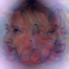
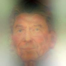
The advantage of using a single image to condition the reconstruction is the possibility to enforce a specific pose, facial expression and background. The disadvantage, is of course, the fact that the final image may contain facial features corresponding to both the embedding and the guiding image. For very low values of the guiding image regularizer weight , the produced image does not look realistic and frequently consists of numerous face fragments. In contrast, for large , the reconstruction may be almost indistinguishable from the guiding image. By tuning the value , it is, however, possible to produce realistic looking faces with barely any facial features “leaked” from the guiding image (see Sec. 3). In Appendix A, we also discuss an alternative approach, in which the regularizer uses a collection of images (with faces sharing a common pose) instead of a single guiding image. This regularizer does not force any specific facial features, but generally results in lower-quality images.
Numerical optimization of Eq. (1) frequently produces noisy and distorted images. This problem can be alleviated by introducing additional regularizers. We use the total-variation (TV) regularizer [14]:
| (2) |
which can be seen to penalize images with high-frequency noise, large gradients and sharp boundaries. Here, and are operators shifting the entire image by pixel in or direction correspondingly and is a constant parameter.
The choice of the optimization function can have a strong impact on the produced face reconstructions. In this paper, we consider two families of loss functions defined on normalized or unnormalized embedding spaces. The first one is based on metric in the embedding space, i. e., . Another approach, which was shown to frequently result in higher-quality images, employs a dot-product: .
3 Iterative face reconstruction
Provided with an embedding and a chosen set of regularizer parameters, the minimization problem (1) can be solved numerically using stochastic gradient descent (SGD), Adam [16], or another optimization method starting from a random noise or the guiding image entering .
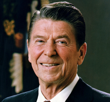
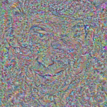
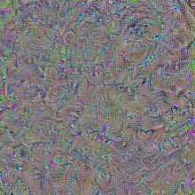
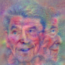
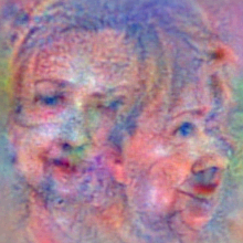
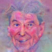
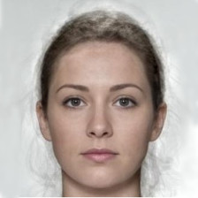
Without any regularizers, the iterative process converges to an image from within a small neighborhood of the initial state [14, 12]. Performing an optimization with the guiding image regularization alone was also unsuccessful at reconstructing a realistic face image. A significant improvement was observed once the total-variation regularizer (2) was introduced in Eq. (1) (see Figs. 1(f), 1(g)). The initial state of the reconstruction was also shown to play an important role: starting with the guiding image instead of a random noise frequently improved both the stability and the quality of the produced images (see Figs. 1(e), 1(f)).
Interestingly, using a sufficiently high allowed us to generate realistic images with facial features of the embedding and the facial expression of the guiding image. By running the algorithm on a sequence of video frames, we were able to perform a “face transfer” from the embedding onto the face shown in the video. This result is particularly impressive given that the embedding can be produced from just a single photo of a person.
The positive effect of the TV regularizer has been previously observed, for example, in Ref. [14]. One can speculate that it can be attributed to suppresion of high-frequency harmonics leading to the search for a local minimum in a subspace of smooth images. Indeed, can be shown to be proportional to , where is the discrete Laplacian operator defined as . If the gradient descent step size is sufficiently small, the expression for the SGD update , can be viewed as a discretization of a dynamical system with a continuous step number , where the regularizer plays a role of the diffusion term:
| (3) |
Here is the sum of embedding and guiding image loss functions, which we ultimately need to minimize. Notice that as shown in Appendix B, in the limit , there are generally a finite number of local minima of and they no longer form high-dimensional submanifolds of .
The total-variation regularizer proved to be essential essential for converging towards a realistic face image, however, it also blurs the output images. We reduced the blurring effect in the produced reconstruction by reducing with the iteration number. Further we also used laplacian pyramid normalization [11] applied to intermediate gradients. This improved overall contrast of the image.
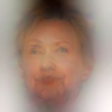
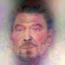
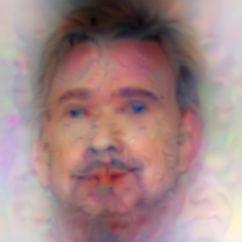
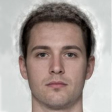
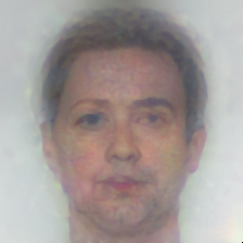
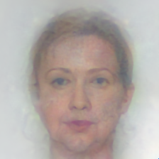
The choice of the guiding image had also proven to be very important for a high quality face reconstruction. When the guiding image and the embedding corresponded to people of different gender or nationality, the produced images could resemble the guiding image with only some facial features “borrowed” from the embedding (see Figs. 2(d), 2(e)). This effect was less noticeable for very large values of , but in this case, the reconstructions had worse quality and were unstable, i. e., could be drastically different for different random initial conditions (sometimes producing images with percievably wrong gender or age). The problem of the guiding image choice can be solved by either building a classifier which predicts the gender and nationality of the face corresponding to a given embedding (and thus prediciting a proper guiding image to be used in the algorithm), or attempting to produce reconstructions with different guiding images and choosing the result with the smallest embedding space distance.



4 Feed-forward network for face reconstruction
Each reconstruction obtained using the methods discussed in Sec. 3, requires hundreds or even thousands of iterations. Training a feed-forward neural network capable of reconstructing an image in a single pass could have a significant performance advantage. The main idea behind training such a network is based on using the same loss function, which we employed for the iterative face reconstruction. Specifically, on each training step, given a random input embedding , the network weights are updated to minimize the loss (1) calculated on and the image produced by the network.
4.1 Feed-forward network taking embedding as an input
The feed-forward network we used for face reconstruction took a -dimensional vector as an input and produced a image with 3 channels (see Fig. 3(a)). Within the network, a fully-connected layer (followed by a ReLU nonlinearity) was first used to transform the embedding vector into a tensor (with 16 being the number of “filters”). This tensor had then been passed through a sequence of ReLU deconvolutions, each of which took an input tensor of size and producing a tensor of the size . In our experiments, the deconvolution kernel had a size and all except for the last one with were equal. The final tensor had been cropped to the fit the FaceNet dimensions of . Using the same loss function which we used for iterative reconstruction, we could then train such a network to produce a face-like image with a desired FaceNet embedding.
4.2 Feed-forward network with an embedding and a guiding image as inputs
A feed-forward network described in Sec. 4.1 can be trained to perform face reconstruction with a set of guiding images instead of one. In this case, a sparse guiding image index can be passed to the network as one of its inputs. Unfortunately, due to a finite capacity of the network and a need to somehow encode all guiding images in the network weights, this could only be demonstrated for a few, but not even dozens of similar guiding images (taken from frames of a video clip). One of the approaches to alleviating this restriction and potentially performing face reconstruction with an arbitrary guiding image is based on passing the guiding image as one of the inputs to the feed-forward neural network.

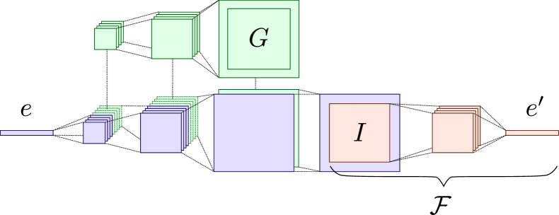
In our experiments, the input guiding image was first padded to the size of and then passed through series of convolutional layers of stride (see Fig. 3(b)). Obtained tensors of size were then depth-concatenated with the tensors of the same spatial dimensions produced through series of deconvolutions as described above. In other words, starting with a tensor generated from the embedding vector and the final convolution of the guiding image, each deconvolution consumed a tensor and produced a tensor, which was then concatenated with a tensor obtained from the guiding image. The last tensor was finally transformed by a convolution operation to produce an output image.
5 Experiments
In this section we explore our ability to generate face images using iterative reconstruction with SGD and feed-forward networks. The quality of reconstruction measures the quality of our loss function in finding recognizable faces. Once we are satisfied with the loss function, that is: we are reasonably confident that the gradient descent with such a loss function produces recognizable faces, we turn our attention to feed-forward networks, which are trained to find the optimum of the same loss, but do it in a single pass.
For our experiments where we want to illustrate the recognizability of people, we choose to use famous people in order to maximize recognizability of the reconstructed images. For our guiding images we use publicly available cartoon images from LABEL:public-domain-vectors as well as averaged images from LABEL:face-research-org.
5.1 Iterative Reconstruction
For our experiments we use pre-normalized embedding as an input. Even though, the original FaceNet was trained to differentiate between normalized embeddings and thus ignore the difference in norm, we find that optimizing a match to pre-normalized embedding produces better results. We conjecture that with normalization, SGD favors smaller embedding values, which essentially results in more generic looking image, as illustrated in Fig. 8. For our experiments, we use both and dot product. Dot product produces significantly sharper, but slightly less recognizable images, as demonstrated in Figs. 1. Somewhat surprisingly, using normalized distance (or, equilvalently, normalized dot product), results in much worse reconstructions.

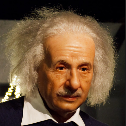
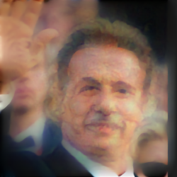
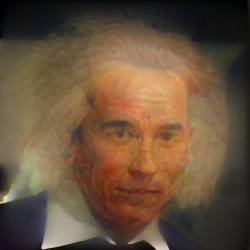
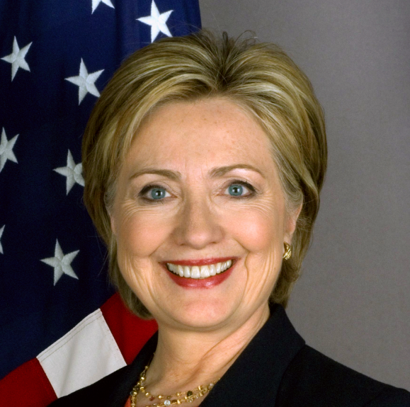
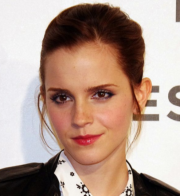
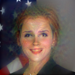

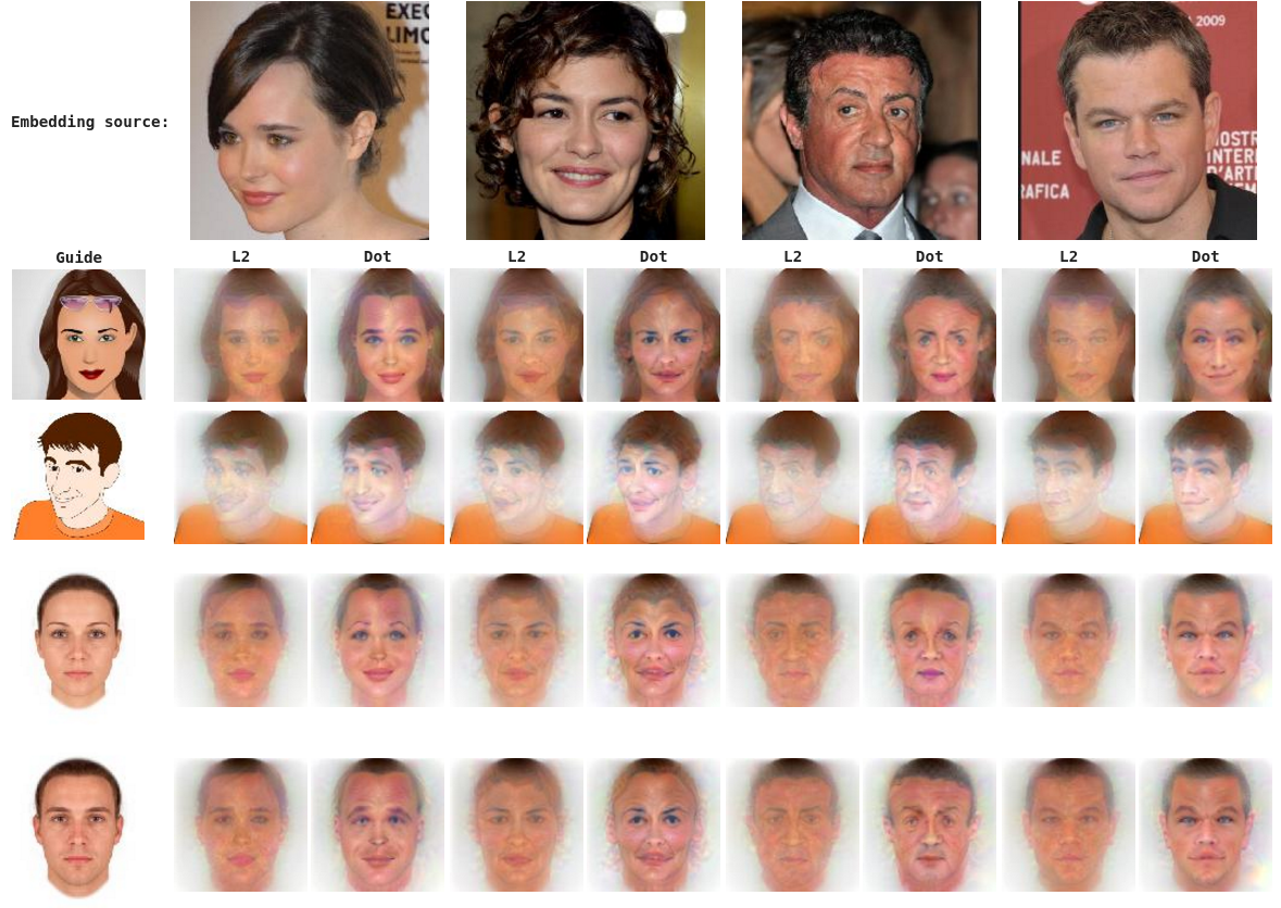
For the example in Fig. 1 we have used activation target on a single intermediate layer. But in the remainder of this section, we attach -distance loss to multiple intermediate layers as well as use Laplacian Pyramid Gradient Normalization [11] to change spectral characteristics of the image gradients. We find that this technique improves the quality of reconstructed images. In figure Fig. 5 we show face reconstructions for multiple celebrities. The guiding images that we use are either cartoon-like faces, or average faces from LABEL:face-research-org. For more face transfer examples including face transfer in a video see supplementary materials.
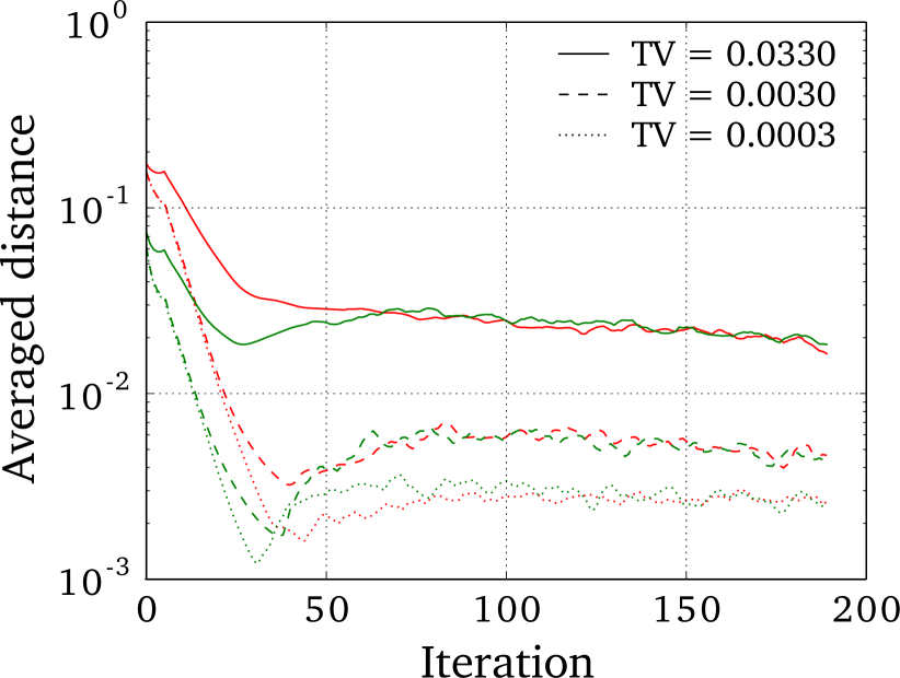
We then turn our attention to the total-variation regularizer. In figures Fig. 6, we show how increasing TV weight affects the image quality. To demonstrate the impact of high TV we did not perform any normalization of the image, which results in very subdued images. It is interesting to note that the embedding of the reconstructed image gets further away from the target as shown in Fig. 6(b) and yet the image becomes more recognizable. Another observation that might be of independent interest is that images in the right-most column of Fig. 6 (the lowest total variation), are extremely similar, and yet each exhibit some traits of the person whose embedding they minimize.



5.2 Feed-forward network
Being trained on a set of embeddings and a single guiding image, the feed-forward network described in Sec. 4.1 taking a FaceNet embedding as an input and producing an image as its output, succesfully converged. The images produced by the network on several embeddings never seen during the training are shown in Fig. 9. The model was observed to converge faster if the network weights were initialized as follows. The deconvolution weights were chosen to produce smooth spatial interpolation with random Xaiver filter-to-filter connections and the final deconvolution was tuned to produce grayscale output image.
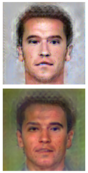
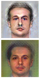
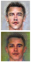
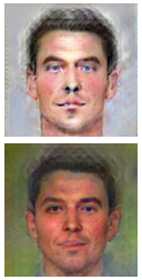
It is remarkable that seemingly similar images produced with the feed-forward network are still recognizible reconstructions of the provided embeddings. This is a demonstration of the fact that only a subtle change of facial features is frequently sufficient to distinguish one person from another.
While in case of iterative reconstruction, there is generally no expectation of the reconstructed image to be smooth, unless we apply a regularizer, for convolutional networks it is smoothness is faciliatedby the fact that lots of parameters are shared across the entire image. One approach quantifying the quality of the constructed feed-forward network is to use the average distance between reconstructed and target embeddings. Note that in contrast with iterative reconstruction, the feed-forward network is unlikely to match input embeddings almost exactly by means of adding just a small perturbation to the guiding image. Indeed, since this additive perturbation is expected to strongly depend on the input embedding, “memorizing” this complicated dependence may require much greater network information capacity than producing accurate smooth reconstructions. On the other hand, the final embedding space loss calculated for images produced by the feed-forward network can be used for choosing optimal model parameters. Table 1 shows average values of the total loss function, embedding space distance and the dot product for the normalized embeddings calculated for several trained feed-forward networks (with distance optimization) on a set of 100 embedding vectors. Even though the feed-forward network seems to perform best with the largest number of filters, using just filters already results in , which is greater than , the average value generally obtained for different real photos of a single person.
| Number of filters | ||||||
|---|---|---|---|---|---|---|
| 50 | 15.098 | 0.0544 | 0.752 | 16.927 | 0.0533 | 0.751 |
| 112 | 12.089 | 0.0407 | 0.804 | 14.798 | 0.0431 | 0.788 |
| 250 | 11.142 | 0.0352 | 0.832 | 11.615 | 0.0400 | 0.808 |
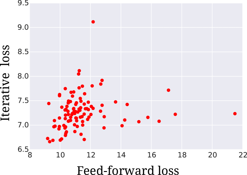
The extent to which the trained feed-forward network optimizes the loss function can be compared to that of the iterative reconstruction algorithm. Figure 10 shows a scatter plot comparing the values of obtained using two approaches. As one would expect, the average of the full loss function calculated for the feed-forward solutions (for embedding space loss and a set of 100 random embeddings) is by a factor of greater than the average loss obtained via iterative reconstruction for the same embeddings. Interestingly, the results of the iterative reconstructions are percieved to be worse than those produced by the feed-forward network. At the same time, the average embedding space distance between the input and output is significantly smaller for the iterative reconstruction.
Feed-forward network with an embedding and a guiding image as inputs
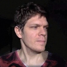
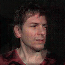
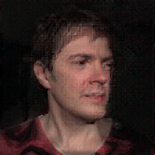
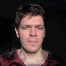
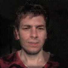
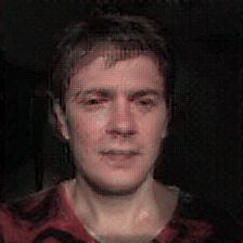
In our experiments, we trained a feed-forward network described in Sec. 4.2 on random embedding vectors and frames of a short video clip treated as a set of independent guiding images. After the network had been trained, we used an embedding vector not seen during the training stage and the same frame sequence to produce an animation. This procedure is generally sucessfull at performing face transfer from the embedding to the target video clip. A few frames from the resulting animation are shown in Fig. 11.
6 Conclusions and future work
We have demonstrated that a FaceNet embedding loss coupled with simple regularization functions can be used to succesfully reconstruct realistic looking faces. Both gradient descent and simple deep neural networks were shown to produce high-quality results. In a way, our work defines two distinct areas that should guide future research. On one hand, we can explore better regularization functions that might improve the quality of the generated images and combine multiple networks for more precise control of the reconstructions. For example, it would be interesting to explore the capability of controlling facial expression of the generated image using a network that was trained to recognize facial expressions (such as anger, satisfaction, smile etc.).
On the other hand, in order to achieve fast generation we need to train a deep network that would solve the minimization problem in one pass. It is interesting that we were able to achieve this without using adversarial learning. This suggests that embedding produced by unrelated network is mostly “complete” in the sense that it contains enough information to reconstruct a recognizable image that matches the original in human understandable sense. An interesting further extension would be to employ more advanced architectures including those utilizing recurrent networks. Also, combining our techniques and adversarial learning is a very promising direction.
Acknowledgments.
The authors thank Alexander Mordvintsev, Blaise Agüera y Arcas, Eider Moore and Florian Schroff for valueable discussions.
References
- [1] Alex Krizhevsky, Ilya Sutskever, and Geoffrey E Hinton. Imagenet classification with deep convolutional neural networks. In Advances in neural information processing systems, pages 1097–1105, 2012.
- [2] Christian Szegedy, Wei Liu, Yangqing Jia, Pierre Sermanet, Scott Reed, Dragomir Anguelov, Dumitru Erhan, Vincent Vanhoucke, and Andrew Rabinovich. Going deeper with convolutions. In Proceedings of the IEEE Conference on Computer Vision and Pattern Recognition, pages 1–9, 2015.
- [3] Kaiming He, Xiangyu Zhang, Shaoqing Ren, and Jian Sun. Deep residual learning for image recognition. 2015. arXiv:cs.CV/1512.03385.
- [4] Florian Schroff, Dmitry Kalenichenko, and James Philbin. FaceNet: A unified embedding for face recognition and clustering. In Proceedings of the IEEE Conference on Computer Vision and Pattern Recognition, pages 815–823, 2015.
- [5] Jonathan Long, Evan Shelhamer, and Trevor Darrell. Fully convolutional networks for semantic segmentation. In Proceedings of the IEEE Conference on Computer Vision and Pattern Recognition, pages 3431–3440, 2015.
- [6] Alec Radford, Luke Metz, and Soumith Chintala. Unsupervised representation learning with deep convolutional generative adversarial networks. 2015. arXiv:cs.LG/1511.06434.
- [7] Alexey Dosovitskiy, Jost Tobias Springenberg, and Thomas Brox. Learning to generate chairs with convolutional neural networks. In IEEE International Conference on Computer Vision and Pattern Recognition, 2014.
- [8] Karol Gregor, Ivo Danihelka, Alex Graves, and Daan Wierstra. Draw: A recurrent neural network for image generation. arXiv preprint arXiv:1502.04623, 2015.
- [9] Leon A. Gatys, Alexander S. Ecker, and Matthias Bethge. A neural algorithm of artistic style. 2015. arXiv:cs.CV/1508.06576.
- [10] Chuan Li and Michael Wand. Combining markov random fields and convolutional neural networks for image synthesis. CoRR, abs/1601.04589, 2016.
- [11] A. Mordvintsev, C. Olah, and M. Tyka. ”deepdream - a code example for visualizing neural networks”, 2015.
- [12] Christian Szegedy, Wojciech Zaremba, Ilya Sutskever, Joan Bruna, Dumitru Erhan, Ian Goodfellow, and Rob Fergus. Intriguing properties of neural networks. 2013. arXiv:cs.CV/1312.6199.
- [13] Ian Goodfellow, Jean Pouget-Abadie, Mehdi Mirza, Bing Xu, David Warde-Farley, Sherjil Ozair, Aaron Courville, and Yoshua Bengio. Generative adversarial nets. In Advances in Neural Information Processing Systems, pages 2672–2680, 2014.
- [14] Aravindh Mahendran and Andrea Vedaldi. Understanding deep image representations by inverting them. In Computer Vision and Pattern Recognition (CVPR), 2015 IEEE Conference on, pages 5188–5196. IEEE, 2015.
- [15] Peter J. Burt and Edward H. Adelson. The laplacian pyramid as a compact image code. IEEE Transactions on Communications, 31(4):532–540, 1983.
- [16] Diederik Kingma and Jimmy Ba. Adam: A method for stochastic optimization. 2014. arXiv:cs.LG/1412.6980.
- [17] publicdomainvectors.org.
- [18] Lisa DeBruine and Ben Jones. ”http://faceresearch.org: Experiments about faces and voice preferences”.
- [19] A. Van der Schaaf and JH van Hateren. Modelling the power spectra of natural images: statistics and information. Vision research, 36(17):2759–2770, 1996.
Appendices
Appendix A Gaussian activation regularizer
Instead of using a single image for regularization, one could consider a collection of photos , faces in which share some characteristics like position, pose or facial expression. Given a function modeling a distribution of images and some constant , the regularizer could, for example, be defined as for and otherwise. However, since many numerical optimization methods perform better on smooth functions, a more practically suitable choice of could be with modelled by a Gaussian distribution in the activation space:
| (4) |
where is a normalization constant, goes over all nodes in the layer , are node activations and , are the average values and standard deviations of the activations computed for all images in . For lower layers , is expected to penalize images with colors or textures inconsistent with those present in the majority of images from . For higher layers, in turn, would give preference to images with the “right” higher-order features.
Notice that given by Eq. (4) can also be thought as a more “natural” way of defining a metric in the activation space. Unlike the guiding image regularizer , which arbitrarily uses an metric, Eq. (4) is invariant under linear rescaling of individual activations.
In practical applications, some of the neural network activations may be almost independent of the network input. Since the corresponding terms dominate , we introduce a small parameter “smoothing” the regularization function and preventing singularities:
| (5) |
where . In our face reconstruction experiments, we used this final form (5) of the regularizer.
In contrast to experiments with a single guiding image, the reconstructions produced with this regularizer do not inherit facial features from any specific pre-defined image. However, they also tend to be less photo-realistic since the average activations include “traces” of numerous images. At lower layers, for example, described a blurred image obtained by superimposing all images from the collection .
Appendix B Local minima of in the limit
The stationary states of Eq. (3) satisfying
| (6) |
where , can be found asymptotically as . Assuming that the shift operators and are cyclic, one can perform a discrete Fourier transformation of :
and the entire equation (6):
| (7) |
where . Since for all non-zero , we can rewrite Eq. (7) as:
| (8) | ||||
| (9) |
where the stationary state is expressed as a sum of a constant component and .
Appendix C Other approaches for improving image quality
Natural images are typically characterized by an intensity power spectrum obeying [19] an approximate power law . The face reconstruction algorithm could be regularized to produce images with a tuned spectrum by performing a Laplacian pyramid (LP) decomposition [15] of the image. Let be the original image, be the “expand” operator and the “reduce” operator [15]. The Laplacian pyramid can then be defined as a sequence of images , where . The LP normalization regularizer
| (12) |
can then favour images with the desired power spectrum and a component norm . An alternative approach is based on normalizing the Laplacian pyramid components of the gradient updates themselves.
In a case when the reconstruction is expected to respect a particular symmetry, the optimization problem Eq. (1) can be regularized to enforce this symmetry. For a special case of a horizontal mirror symmetry, the regularizer could read
where is a horizontal image “flipping” operator.