Light-cone like spreading of single-particle correlations in the Bose-Hubbard model after a quantum quench in the strong coupling regime

Abstract

We study the spreading of correlations in space and time after a quantum quench in the Bose Hubbard model. We derive equations of motion for the single-particle Green’s function within the contour-time formalism, allowing us to study dynamics in the strong coupling regime. We discuss the numerical solutions of these equations and calculate the single-particle density matrix for quenches in the Mott phase. We demonstrate light-cone like spreading of correlations in the Mott phase in one, two, and three dimensions and calculate propagation velocities in each dimension.

I Introduction

The out-of-equilibrium dynamics of interacting quantum systems has become a major subject of interest in many-body physics. Experimental advances have made ultracold atoms in optical lattices offer a promising setting to study out-of-equilibrium phenomena and attracted considerable attention in recent years (Bloch, 2005; Jaksch and Zoller, 2005; Morsch and Oberthaler, 2006; Lewenstein et al., 2007; Bloch et al., 2008; Kennett, 2013). These systems are highly versatile in that experimental parameters can be tuned over a wide range of values in real time. This facilitates the study of quantum quenches, in which parameters in the corresponding Hamiltonian are varied in time faster than the system can respond adiabatically. Such protocols open the door to a rich range of many-body physics and have been studied intensely both theoretically and experimentally.

Jaksch et al. (Jaksch et al., 1998) showed that ultracold bosons trapped in optical lattices can be described by the Bose-Hubbard model (BHM) – a minimal model of interacting bosons on a lattice. The BHM exhibits a quantum phase transition between a superfluid and Mott-insulator as the ratio of the hopping strength, $J$, to the on-site interaction strength, $U$, is varied (Fisher et al., 1989), which was demonstrated experimentally for cold atoms by Greiner et al. (Greiner et al., 2002). This allows for the study of quantum quenches across a quantum critical point, in addition to quenches within a particular phase.

A variety of quench protocols have been suggested and implemented (Greiner et al., 2002; Chen et al., 2011; Hung et al., 2010; Bakr et al., 2010) for the BHM in order to study out of equilibrium phenomena such as the Kibble-Zurek effect Kibble (1976); Zurek (1985); Zurek et al. (2005); Chen et al. (2011) and relaxation after a quench (Clark and Jaksch, 2004; Kollath et al., 2007; Sciolla and Biroli, 2010, 2011; Fischer et al., 2008; Fischer and Schützhold, 2008; Kennett and Dalidovich, 2011; Strand et al., 2015; Landea and Nessi, 2015; Polkovnikov, 2005; Natu et al., 2011; Bernier et al., 2011; Natu and Mueller, 2013; Bernier et al., 2012; Zakrzewski, 2005; Trefzger and Sengupta, 2011; Yanay and Mueller, 2016). Our particular interest here is the light-cone like spreading of correlations after a quantum quench. Several analytical and numerical studies have shown a Lieb-Robinson-like Lieb and Robinson (1972) maximal propagation velocity for the spreading of density correlations in one dimensional systems for quenches from the superfluid to Mott-insulating regime as well as quenches solely within the superfluid (Carleo et al., 2014) or Mott-insulating regimes (Fischer et al., 2008; Bernier et al., 2011; Läuchli and Kollath, 2008; Barmettler et al., 2012; Krutitsky et al., 2014). The latter case was recently observed by Cheneau et al. (Cheneau et al., 2012) for an array of decoupled one-dimensional chains. Some theoretical predictions have also been made for higher dimensional systems (Carleo et al., 2014; Navez and Schützhold, 2010; Natu and Mueller, 2013; Krutitsky et al., 2014) but these have not yet faced experimental scrutiny.

A generic problem in the theoretical description of quantum quenches is that it is necessary to have a formalism that is able to describe the physics in a broad area of parameter space. In the case of the Bose Hubbard model, numerical approaches such as exact diagonalization (ED) and the time-dependent density matrix renormalization group (t-DMRG) Kollath et al. (2007); Läuchli and Kollath (2008); Bernier et al. (2011, 2012); Clark and Jaksch (2004); Cheneau et al. (2012); Trotzky et al. (2012) can be essentially exact in all parts of parameter space but are limited by system size and usually are practical only in one dimension. For dimensions higher than one, methods such as time-dependent Gutzwiller mean field theory Lewenstein et al. (2007); Zakrzewski (2005); Amico and Penna (2000); Natu et al. (2011) and dynamical mean field theory Strand et al. (2015) have been used which can capture the presence of a quantum phase transition, but in their simplest form do not capture spatial correlations. However, there has been work on including perturbative corrections Trefzger and Sengupta (2011); Dutta et al. (2012); Navez and Schützhold (2010); Schroll et al. (2004); Yanay and Mueller (2016); Queisser et al. (2014); Krutitsky et al. (2014) to remedy this weakness.

In previous work (Fitzpatrick and Kennett, 2018), we developed a real-time two-particle irreducible (2PI) effective action approach to the BHM based on a strong-coupling theory of the BHM (Sengupta and Dupuis, 2005; Kennett and Dalidovich, 2011) that is exact in both the weak and strong coupling limits. We verified that by using a Hartree-Fock-Bogoliubov approximation we were able to obtain considerable improvements beyond mean field theory in calculating equilibrium properties of the BHM (Fitzpatrick and Kennett, 2018). We also derived equations of motion for the single-particle Green’s function using the contour-time formalism (Konstantinov and Perel, 1961). In this paper we use the equations of motion to investigate the case of a quench in the Mott-insulating regime. We demonstrate light-cone spreading of single-particle correlations in one, two and three dimensions. We also study the dependence of the maximal propagation velocity on quench protocol, chemical potential, temperature and dimensionality that should be relevant for comparisons with experiment.

The paper is structured as follows. In Sec. II, we describe the model that we study and the theoretical formalism we use to calculate correlations after a quench. In Sec. III, we briefly discuss the equations of motion for the single-particle Green’s function that we obtained in our previous work (Fitzpatrick and Kennett, 2018) and show how they simplify for quenches that are confined to the Mott regime. In Sec. IV, we present numerical results obtained from integrating the quations of motion and finally in Sec. V, we discuss our results and present our conclusions.

II Model and Formalism

In this section we introduce the Bose-Hubbard model and the effective theory we use to study quench dynamics in the strong-coupling regime, all within the context of the contour-time formalism. The Hamiltonian for the BHM, allowing for a time dependent hopping term, is

$$\hat{H}_{\text{BHM}}\left(t\right)=\hat{H}_{J}\left(t\right)+\hat{H}_{0},$$ (1)

where

$$\hat{H}_{J}\left(t\right)=-\sum_{\left\langle\vec{r}_{1},\vec{r}_{2}\right\rangle}J_{\vec{r}_{1}\vec{r}_{2}}\left(t\right)\left(\hat{a}_{\vec{r}_{1}}^{\dagger}\hat{a}_{\vec{r}_{2}}+\hat{a}_{\vec{r}_{2}}^{\dagger}\hat{a}_{\vec{r}_{1}}\right),$$ (2)

and

$$\hat{H}_{0}=\hat{H}_{U}-\mu\hat{N}=\frac{U}{2}\sum_{\vec{r}}\hat{n}_{\vec{r}}\left(\hat{n}_{\vec{r}}-1\right)-\mu\sum_{\vec{r}}\hat{n}_{\vec{r}},$$ (3)

with $\hat{a}_{\vec{r}}^{\dagger}$ and $\hat{a}_{\vec{r}}$ annihilation and creation operators for bosons on lattice site $\vec{r}$ respectively, $\hat{n}_{\vec{r}}\equiv\hat{a}_{\vec{r}}^{\dagger}\hat{a}_{\vec{r}}$ the number operator, $U$ the interaction strength, and $\mu$ the chemical potential. The notation $\left\langle\vec{r}_{1},\vec{r}_{2}\right\rangle$ indicates a sum over nearest neighbours only. We allow $J_{\vec{r}_{1}\vec{r}_{2}}\left(t\right)$, the hopping amplitude between sites $\vec{r}_{1}$ and $\vec{r}_{2}$, to be time dependent. We have specified the model for a uniform lattice, but could consider a trap as is used in experiment by introducing a site-dependent chemical potential. This leads to more complicated calculations than we consider here but is conceptually straightforward to include.

II.1 Contour-time formalism

The general formalism that we discuss and adopt in this paper was developed in a previous paper of ours; we refer the reader to Ref. (Fitzpatrick and Kennett, 2018) for details on the formalism. We use the contour-time formalism (Schwinger, 1961; Keldysh, 1964; Rammer and Smith, 1986; Niemi and Semenoff, 1984; Landsman and van Weert, 1987; Chou et al., 1985), which treats time as a complex variable lying along a contour in a way that allows the description of out-of-equilibrium and equilibrium quantum phenomena within the same formalism. For systems initially prepared in thermal states, which we consider here, one can work with a contour $C$ of the form illustrated in Fig. 1 which is sometimes referred to as the Konstantinov and Perel’ (KP) contour (Konstantinov and Perel, 1961). A popular alternative to the KP contour is the Schwinger-Keldysh (SK) closed-time path (Schwinger, 1961; Keldysh, 1964) which is also suitable for initially thermalized systems. However, unlike the KP contour, the SK contour ignores transient phenomena, being more suitable for calculating steady states or other long-time phenomena. Given that transient effects are important in the spreading of space-time correlations after a quantum quench, the KP contour is a more appropriate choice. A number of authors have applied contour-time approaches to the BHM in out-of-equilibrium scenarios (Robertson et al., 2011; Dalidovich and Kennett, 2009; Fitzpatrick and Kennett, 2018; Kennett and Dalidovich, 2011; Graß et al., 2011a, b; Graß, 2009; Rey et al., 2004, 2005; Temme and Gasenzer, 2006; Calzetta et al., 2006; Polkovnikov, 2003; Lo Gullo and Dell’Anna, 2016) – our work differs from previous approaches (Rey et al., 2004; Temme and Gasenzer, 2006) in that we apply an effective theory to the BHM within the contour formalism that is appropriate for strong coupling as well as weak coupling (Kennett and Dalidovich, 2011; Fitzpatrick and Kennett, 2018).

Figure 1: Contour for a system initially prepared at time $t_{i}$ in a thermal state with inverse temperature $\beta$. $t_{f}$ is the maximum real-time considered in the problem, which may be set to $t_{f}\to\infty$ without loss of generality.

II.2 Contour-ordered Green’s functions

To characterize spatio-temporal correlations in the BHM we calculate contour-ordered Green’s functions (COGFs). We define the $n$-point COGF as (Chou et al., 1985)

$$G_{\vec{r}_{1}\ldots\vec{r}_{n}}^{a_{1}\ldots a_{n}}\left(\tau_{1},\ldots,\tau_{n}\right) \equiv\left(-i\right)^{n-1}\text{Tr}\left\{\hat{\rho}_{i}T_{C}\left[\hat{a}_{\vec{r}_{1}}^{a_{1}}\left(\tau_{1}\right)\ldots\hat{a}_{\vec{r}_{n}}^{a_{n}}\left(\tau_{n}\right)\right]\right\}$$

$$\equiv\left(-i\right)^{n-1}\left\langle T_{C}\left[\hat{a}_{\vec{r}_{1}}^{a_{1}}\left(\tau_{1}\right)\ldots\hat{a}_{\vec{r}_{n}}^{a_{n}}\left(\tau_{n}\right)\right]\right\rangle_{\hat{\rho}_{i}},$$ (4)

where $\hat{\rho}_{i}$ is the state operator for a thermal state representing the initial state of our system:

$$\hat{\rho}_{i}=\frac{e^{-\beta\hat{H}_{\text{BHM}}\left(t_{i}\right)}}{\text{Tr}\left\{e^{-\beta\hat{H}_{\text{BHM}}\left(t_{i}\right)}\right\}},$$ (5)

the $a_{i}$ upper indices are defined such that

$$\hat{a}_{\vec{r}}^{1}\equiv\hat{a}_{\vec{r}},\quad\hat{a}_{\vec{r}}^{2}\equiv\hat{a}_{\vec{r}}^{\dagger},$$ (6)

and $\hat{a}_{\vec{r}}^{a}\left(\tau\right)$ are the bosonic fields in the Heisenberg picture with respect to $\hat{H}_{\text{BHM}}\left(\tau\right)$ [Eq. (1)]:

$$\hat{a}_{\vec{r}}^{a}\left(\tau\right) =U^{\dagger}\left(\tau,\tau_{i}\right)\hat{a}_{\vec{r}}^{a}U\left(\tau,\tau_{i}\right),$$ (7)

$$U\left(\tau,\tau^{\prime}\right) =T_{C}\left[e^{-\int_{C\left(\tau,\tau^{\prime}\right)}d\tau^{\prime\prime}\hat{H}_{\text{BHM}}\left(\tau^{\prime\prime}\right)}\right].$$ (8)

Here we have introduced explicitly the complex contour time argument $\tau$, the sub-contour $C\left(\tau,\tau^{\prime}\right)$ which goes from $\tau$ to $\tau^{\prime}$ along the contour $C$, and the contour time ordering operator $T_{C}$, which orders strings of operators according to their position on the contour, with operators at earlier contour times placed to the right.

II.3 Effective theory for the Bose-Hubbard model

In order to study quench dynamics in the BHM, we make use of an effective theory (expressed as an action) that can describe both the weak and strong coupling limits of the model in the same formalism. Such an approach was developed in imaginary time by Sengupta and Dupuis (Sengupta and Dupuis, 2005) by using two Hubbard-Stratonovich transformations, then generalized to the SK contour in Ref. (Kennett and Dalidovich, 2011), and then further generalized to the KP contour in Ref. (Fitzpatrick and Kennett, 2018) in conjunction with a 2PI effective action approach. A similar real-time theory was also obtained based on a Ginzburg-Landau approach using the Schwinger-Keldysh technique (Graß et al., 2011a, b; Graß, 2009) in conjunction with a one-particle irreducible (1PI) effective action approach. In obtaining the effective theory below, one assumes that the system is dominated by the low-energy degrees of freedom, which is valid as along as the quench is sufficiently slow. A detailed discussion of the development of the effective theory within the KP contour formalism is presented in Ref. (Fitzpatrick and Kennett, 2018). The effective theory obtained in Ref. (Fitzpatrick and Kennett, 2018) for $z$ fields (which are obtained after two Hubbard Stratonovich transformations and have the same correlations as the original $a$ fields (Sengupta and Dupuis, 2005)) is

$$S\left[z\right] =\frac{1}{2!}\sum_{\vec{r}}\int_{C}\int_{C}d\tau_{1}d\tau_{2}\left[\mathcal{G}^{-1}\right]^{a_{1}a_{2}}\left(\tau_{1},\tau_{2}\right)z_{\vec{r}}^{\overline{a_{1}}}\left(\tau_{1}\right)z_{\vec{r}}^{\overline{a_{2}}}\left(\tau_{2}\right)$$

$$\quad+\frac{1}{2!}\sum_{\vec{r}_{1}\vec{r}_{2}}\int_{C}d\tau\left\{2J_{\vec{r}_{1}\vec{r}_{2}}\left(\tau\right)+\delta_{\vec{r}_{1}\vec{r}_{2}}v_{1}\right\}\sigma_{1}^{a_{1}a_{2}}z_{\vec{r}_{1}}^{\overline{a_{1}}}\left(\tau\right)z_{\vec{r}_{2}}^{\overline{a_{2}}}\left(\tau\right)$$

$$\quad+\frac{1}{4!}\sum_{\vec{r}}\int_{C}d\tau\left\{-2u_{1}\right\}\sigma^{a_{1}a_{2}a_{3}a_{4}}z_{\vec{r}}^{\overline{a_{1}}}\left(\tau\right)z_{\vec{r}}^{\overline{a_{2}}}\left(\tau\right)z_{\vec{r}}^{\overline{a_{3}}}\left(\tau\right)z_{\vec{r}}^{\overline{a_{4}}}\left(\tau\right),$$ (9)

where $\mathcal{G}^{a_{1}a_{2}}\left(\tau_{1},\tau_{2}\right)$ is the atomic (i.e. $J=0$) two-point Green’s function (see Appendix C of Ref. (Fitzpatrick and Kennett, 2018) for the full expression), $u_{1}$ is a complicated function of the inverse temperature $\beta$ and the chemical potential $\mu$ (see Appendix D of Ref. (Fitzpatrick and Kennett, 2018) for the full expression), and

$$v_{1} =\left(2n_{J=0}+1\right)u_{1},$$ (10)

where $n_{J=0}$ is the average particle density in the atomic limit. This can be calculated from the atomic kinetic Green’s function $\mathcal{G}^{12,\left(K\right)}$ (see Appendix C of Ref. (Fitzpatrick and Kennett, 2018)) as follows

$$n_{J=0} =\frac{1}{2}\left\{i\mathcal{G}_{\vec{k}}^{12,\left(K\right)}\left(t^{\prime}=0\right)-1\right\}.$$ (11)

the overscored index $\overline{a}$ used in Eq. (9) is defined by

$$f_{\vec{r}}^{\overline{a}}\left(\tau\right)\equiv\sigma_{1}^{aa^{\prime}}f_{\vec{r}}^{a^{\prime}}\left(\tau\right),$$ (12)

where $\sigma_{i}$ is the $i^{\text{th}}$ Pauli matrix, i.e. $\overline{1}=2$ and $\overline{2}=1$, and

$$\sigma^{a_{1}a_{2}a_{3}a_{4}}\equiv\begin{cases}1,&\text{if }\left\{a_{m}\right\}_{m=1}^{4}\in P\left(\left\{1,1,2,2\right\}\right)\\ 0,&\text{otherwise}\end{cases}.$$ (13)

We use the Einstein summation convention for the Nambu indices, i.e. matching indices implies a summation over all possible values of those indices.

When applied to an nPI effective action approach, where one ultimately calculates equations of motion for various different correlation functions, the effective theory generates “anomalous” Feynman diagrams (Dupuis, 2001; Sengupta and Dupuis, 2005; Kennett and Dalidovich, 2011; Fitzpatrick and Kennett, 2018; Sajna and Micnas, 2018). These diagrams contain internal inverse atomic propagator lines which do not correspond to any physical processes. If one considers all orders of the theory, they can be dropped because the different anomalous terms cancel. If the theory is truncated (as is usually the case), then care is required to ensure cancellation order by order. At the level considered here, the $v_{1}$ term in Eq. (9) plays this role. For a more detailed discussion of the cancellation of anomalous diagrams, see Ref. (Fitzpatrick and Kennett, 2018).

The effective theory introduces an effective potential $v_{1}$ and a renormalized on-site interaction strength $u_{1}$. Moreover, it reassigns the role of the “bare propagator” to the atomic propagator. The theory gives the exact two-point connected COGF (CCOGF) in both the atomic and noninteracting limits, thus making it particularly appealing for the study of quench dynamics since it gives a reasonable description of the behaviour of the system in both the superfluid and Mott-insulating regimes (Kennett, 2013).

III Equations of motion

Our goal is to calculate the full two-point CCOGF (the “full propagator” from now on) after a quench, which encodes non-local single-particle spatial and temporal correlations. To achieve this, we solve the Dyson’s equation (Cornwall et al., 1974; Fitzpatrick and Kennett, 2018) for the full propagator (the superscript “c” indicates that $G$ is a connected COGF):

$$G_{\vec{k}}^{a_{1}a_{2},c}\left(\tau_{1},\tau_{2}\right)\equiv\left[G_{0}\right]_{\vec{k}}^{a_{1}a_{2},c}\left(\tau_{1},\tau_{2}\right)+\int_{C}\int_{C}d\tau_{3}d\tau_{4}\left[G_{0}\right]_{\vec{k}}^{a_{1}a_{3},c}\left(\tau_{1},\tau_{3}\right)\Sigma_{\vec{k}}^{\overline{a_{3}}\overline{a_{4}}}\left(\tau_{3},\tau_{4}\right)G_{\vec{k}}^{a_{4}a_{2},c}\left(\tau_{4},\tau_{2}\right),$$ (14)

where $G_{0}$ is the bare propagator and $\Sigma$ is the self-energy of the theory. Since we consider a translationally invariant system, we work in quasi-momentum space rather than real space. In Ref. (Fitzpatrick and Kennett, 2018), we calculated the self-energy for the effective theory [Eq. (9)] in a systematic way using a 2PI effective action approach (Cornwall et al., 1974) and considered terms up to first order in $u_{1}$ (loosely corresponding to a Hartree-Fock-Bogoliubov (HFB) like approximation).

The equations of motion derived in Ref. (Fitzpatrick and Kennett, 2018) are quite general in that they can be applied to a variety of different quench protocols. Here we consider the case in which the hopping quench is restricted to the Mott-insulating regime and the system is initially thermalized in the atomic limit. Under these conditions, the self-energy (and thus the equations of motion) simplify considerably, and it is straightforward to show that the equations of motion derived in Ref. (Fitzpatrick and Kennett, 2018) reduce to

$$A_{\vec{k}}\left(t,t^{\prime}\right) =\mathcal{A}\left(t-t^{\prime}\right)-i\int_{t^{\prime}}^{t}dt^{\prime\prime}\mathcal{A}\left(t-t^{\prime\prime}\right)\Sigma_{\vec{k}}^{\left(HFB\right)}\left(t^{\prime\prime}\right)A_{\vec{k}}\left(t^{\prime\prime},t^{\prime}\right),$$ (15)

$$G_{\vec{k}}^{\left(K\right)}\left(t,t^{\prime}\right) =\mathcal{G}^{\left(K\right)}\left(t-t^{\prime}\right)-i\int_{0}^{t}dt^{\prime\prime}\mathcal{A}\left(t-t^{\prime\prime}\right)\Sigma_{\vec{k}}^{\left(HFB\right)}\left(t^{\prime\prime}\right)G_{\vec{k}}^{\left(K\right)}\left(t^{\prime\prime},t^{\prime}\right)$$

$$\quad+i\int_{0}^{t^{\prime}}dt^{\prime\prime}\mathcal{G}^{\left(K\right)}\left(t-t^{\prime\prime}\right)\Sigma_{\vec{k}}^{\left(HFB\right)}\left(t^{\prime\prime}\right)A_{\vec{k}}\left(t^{\prime\prime},t^{\prime}\right),$$ (16)

where $A_{\vec{k}}\left(t,t^{\prime}\right)$ is the spectral function:

$$A_{\vec{k}}\left(t,t^{\prime}\right)=\left\langle\hat{a}_{\vec{k}}\left(t\right)\hat{a}_{\vec{k}}^{\dagger}\left(t^{\prime}\right)-\hat{a}_{\vec{k}}^{\dagger}\left(t^{\prime}\right)\hat{a}_{\vec{k}}\left(t\right)\right\rangle_{\hat{\rho}_{i}},$$ (17)

and $G_{\vec{k}}^{\left(K\right)}\left(t,t^{\prime}\right)$ is the kinetic Green’s function:

$$G_{\vec{k}}^{\left(K\right)}\left(t,t^{\prime}\right) =G_{\vec{k}}^{12,\left(K\right)}\left(t,t^{\prime}\right)$$

$$=-i\left\langle\hat{a}_{\vec{k}}\left(t\right)\hat{a}_{\vec{k}}^{\dagger}\left(t^{\prime}\right)+\hat{a}_{\vec{k}}^{\dagger}\left(t^{\prime}\right)\hat{a}_{\vec{k}}\left(t\right)\right\rangle_{\hat{\rho}_{i}}.$$ (18)

The quantities $\mathcal{A}\left(t-t^{\prime}\right)$ and $\mathcal{G}^{\left(K\right)}\left(t-t^{\prime}\right)$ that enter Eqs. (15) and (16) are the spectral function in the atomic limit and the kinetic Green’s function in the atomic limit respectively. In this limit both quantities are time-translational invariant. $\Sigma_{\vec{k}}^{\left(HFB\right)}\left(t\right)$ is the self-energy in the HFB approximation:

$$\Sigma_{\vec{k}}^{\left(HFB\right)}\left(t\right)=\epsilon_{\vec{k}}\left(t\right)+2u_{1}\left\{n\left(t\right)-n_{J=0}\right\},$$ (19)

with

$$\epsilon_{\vec{k}}\left(t\right) =-2J\left(t\right)\sum_{i=1}^{d}\cos\left(k_{i}a\right),$$ (20)

$$n\left(t\right) =\frac{1}{N_{\text{sites}}}\sum_{\vec{k}}n_{\vec{k}}\left(t\right),$$ (21)

$$n_{\vec{k}}\left(t\right) =\frac{1}{2}\left\{iG_{\vec{k}}^{\left(K\right)}\left(t,t\right)-1\right\},$$ (22)

and $a$ the lattice constant (assuming a $d$-dimensional hypercube geometry). In the atomic limit, the spectral function and kinetic Green’s functions can be written as

$$\mathcal{A}\left(t\right) =\frac{1}{\mathcal{Z}}\sum_{n=0}^{\infty}e^{-\beta\left(\mathcal{E}_{n}-\mathcal{E}_{n_{\text{MI}}}\right)}\left\{\left(n+1\right)e^{-i\left(\mathcal{E}_{n+1}-\mathcal{E}_{n}\right)t}-ne^{i\left(\mathcal{E}_{n-1}-\mathcal{E}_{n}\right)t}\right\},$$ (23)

$$\mathcal{G}^{\left(K\right)}\left(t\right) =-\frac{i}{\mathcal{Z}}\sum_{n=0}^{\infty}e^{-\beta\left(\mathcal{E}_{n}-\mathcal{E}_{n_{\text{MI}}}\right)}\left\{\left(n+1\right)e^{-i\left(\mathcal{E}_{n+1}-\mathcal{E}_{n}\right)t}+ne^{i\left(\mathcal{E}_{n-1}-\mathcal{E}_{n}\right)t}\right\},$$ (24)

where $\mathcal{E}_{n}$ is the single-site energy:

$$\mathcal{E}_{n}=\frac{U}{2}n\left(n-1\right)-\mu n,$$ (25)

$n_{\text{MI}}$ is the zero-temperature particle density:

$$n_{\text{MI}}=\left\lceil\mu/U\right\rceil,$$ (26)

and $\mathcal{Z}$ is the partition function:

$$\mathcal{Z}=\sum_{n=0}^{\infty}e^{-\beta\left(\mathcal{E}_{n}-\mathcal{E}_{n_{\text{MI}}}\right)}.$$ (27)

We consider quenches in which the hopping amplitude $J\left(t\right)$ is tuned as a function of time. [Experimentally this corresponds to varying the depth of the optical lattice, since hopping varies exponentially with lattice depth while interactions vary weakly with lattice depth (Zwerger, 2003).] We choose $J\left(t\right)$ to have the following form:

$$J\left(t\right)=\left(\frac{J_{f}-J_{i}}{2}\right)\tanh\left(\frac{t-t_{c}}{\tau_{Q}}\right)+\left(\frac{J_{f}+J_{i}}{2}\right),$$ (28)

which corresponds to the experimental scenario of a linear ramp. Note that $\lim_{t\to-\infty}J\left(t\right)=J_{i}$, and $\lim_{t\to\infty}J\left(t\right)=J_{f}$. The time scale $\tau_{Q}$ is the characteristic time for $J\left(t\right)$ to cross from $J_{i}$ to $J_{f}$, and $t_{c}$ is the time at which the middle of the quench is occurring. Other forms of $J\left(t\right)$ which are not linear may lead to differing behaviour in the long-time limit (Sen et al., 2008). For the quench scenario we consider in this paper, $J_{c}>J_{f}>J_{i}=0$, where $J_{c}$ is the critical hopping strength at the superfluid to Mott insulator phase boundary (for fixed $\mu$).

IV Numerical Results

The equations of motion, Eqs. (15) and (16), form a system of nonlinear Volterra integral equations that have no known analytical solution, hence we take a numerical approach to solve them. This presents more of a challenge than the one-particle-irreducible (1PI) equations of motion obtained in Ref. (Kennett and Dalidovich, 2011) due to the presence of memory kernels that incorporate the entire history of the system, making explicit the importance of the quench protocol to the post-quench state. An additional important feature of the equations of motion is that they are causal, i.e. all quantities at some later time $t_{f}$ can be obtained by integration over the known functions for times $t\leq t_{f}$. We exploit this feature of the equations to develop an implicit block-by-block scheme, closely following Ref. (Katani and Shahmorad, 2010). A detailed discussion of our numerical scheme is presented in Appendix A.

In this section we first compare the results of the solutions of Eqs. (15) and (16) to exact diagonalization (ED) calculations. Obtaining acceptable agreement we then present numerical results for the light-cone like propagation of single-particle spatial correlations in one, two, and three dimensions for quenches in the Mott insulating regime.

IV.1 Comparison to exact diagonalization calculations

First, we assess the accuracy of our effective theory by comparing calculations of the single-particle density matrix $\rho_{1}\left(\Delta\vec{r},t\right)$ obtained from this theory to that from exact diagonalization calculations for small system sizes. $\rho_{1}\left(\Delta\vec{r},t\right)$ is a natural quantity to study single-particle spatial correlations, which can be calculated from the equal-time kinetic Green’s function $G_{\vec{k}}^{\left(K\right)}\left(t,t\right)$ as follows:

$$\rho_{1}\left(\Delta\vec{r},t\right) =\frac{1}{N_{\text{sites}}}\sum_{\vec{k}}\cos\left(\vec{k}\cdot\Delta\vec{r}\right)n_{\vec{k}}\left(t\right)$$

$$=\frac{1}{2N_{\text{sites}}}\sum_{\vec{k}}\cos\left(\vec{k}\cdot\Delta\vec{r}\right)\left\{iG_{\vec{k}}^{\left(K\right)}\left(t,t\right)-1\right\}.$$ (29)

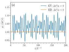
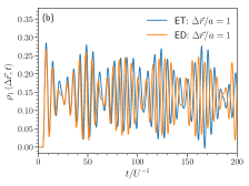
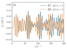
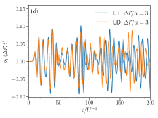
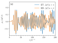
Figure 2: (Color online) (a)-(e) Comparison of $\rho_{1}\left(\Delta\vec{r},t\right)$ obtained by our ET and by ED for $\Delta\vec{r}/a=0$ to $4$ respectively. The parameters are $\beta U=\infty$, $\mu/U=0.4116$, $J_{f}/U=0.035$, $t_{c}/U^{-1}=5$, $\tau_{Q}/U^{-1}=0.1$, $d=1$, and $N_{s}=8$.

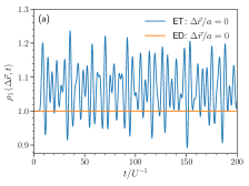
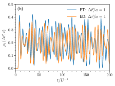
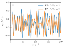
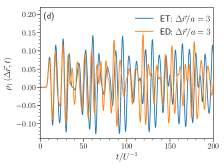
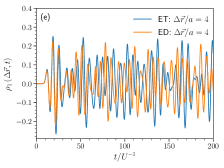
Figure 3: (Color online) (a)-(e) Comparison of $\rho_{1}\left(\Delta\vec{r},t\right)$ obtained by our ET and by ED for $\Delta\vec{r}/a=0$ to $4$ respectively. The parameters are the same as in Fig. 2 except that $J_{f}/U=0.05$.

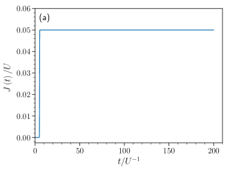
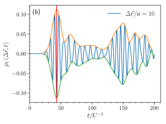
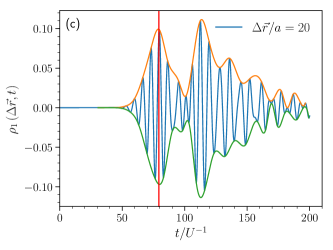
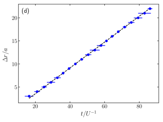
Figure 4: (Color online) (a) The evolution of $J\left(t\right)/U$ for quench parameters $J_{f}/U=0.05$, $t_{c}/U^{-1}=5$, and $\tau_{Q}/U^{-1}=0.1$; (b) dynamics of $\rho_{1}\left(\Delta\vec{r},t\right)$ for $\Delta\vec{r}/a=10$; (c) dynamics of $\rho_{1}\left(\Delta\vec{r},t\right)$ for $\Delta\vec{r}/a=20$; (d) scatter plot of the time $t/U^{-1}$ it takes for the single-particle correlation front to travel a distance $\Delta r/a$. We show a straight line fit to the data. In (b) and (c), the orange and green lines trace the envelopes of the wavepackets while the red line estimates the position of the centre of the first wavepacket. The parameters for (b)-(d) include the quench parameters in (a), as well as $\mu/U=0.4116$, $\beta U=1000$, $d=1$, and $N_{s}=50$.

In Figs. 2 and 3, we display the time evolution of $\rho_{1}\left(\Delta\vec{r},t\right)$, obtained from both the effective theory (ET) and ED, for a quench performed on an 8-site chain ($d=1$; $N_{s}=8$) with $\beta=\infty$ ($T=0$), $\mu/U=0.4116$, $t_{c}/U^{-1}=5$, and $\tau_{Q}/U^{-1}=0.1$. The only differing parameter between the two figures is the final hopping strength $J_{f}/U$, where $J_{f}/U=0.035$ for Fig. 2 and $J_{f}/U=0.05$ for Fig. 3.

Figure 2(a) plots $\rho_{1}\left(\Delta\vec{r},t\right)$ for $\Delta\vec{r}/a=0$, which is equivalent to the average particle density. Figure 2(a) shows that our effective theory leads to small fluctuations in the particle number, typically on the order of 5%. In Appendix B, we discuss the origin of these particle number fluctuations. The results in Figs. 2(b)-(e) show that this disagreement with ED is confined to $\Delta\vec{r}/a=0$ since for $\Delta\vec{r}/a\neq 0$ our method is quantitatively accurate for times up to $\sim 100\,U^{-1}$. At later times, the beats calculated by our method, begin to become out of phase with those obtained by ED.

Figures 3(a)-(e) display the time evolution of $\rho_{1}\left(\Delta\vec{r},t\right)$ for an identical system to that shown in Figs. 2(a)-(e) except that $J_{f}/U=0.05$. For this value of $J_{f}$, the ET is quantitatively accurate for times up to $\sim 50\,U^{-1}$ when $\Delta\vec{r}/a\neq 0$. This is a sufficiently long time window to allow the identification of the peak of the first wavepacket in $\rho_{1}\left(\Delta\vec{r},t\right)$ at a given $\Delta\vec{r}/a\neq 0$, which we use to determine the velocity at which single particle correlations spread. The good agreement with ED results in 8 site systems gives us confidence in the results we obtain in larger systems and higher dimensions where comparison with ED is not possible.

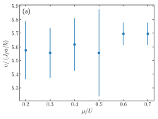
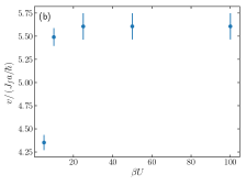
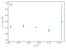
Figure 5: (Color online) Scatter plots of the propagation velocity $v/\left(J_{f}a/\hbar\right)$ in one dimension as a function of various model parameters. In all cases $t_{c}/U^{-1}=5$, and $\tau_{Q}/U^{-1}=0.1$. (a) scatter plot of $v/\left(J_{f}a/\hbar\right)$ as a function of $\mu/U$ for a 50 site chain with $\beta U=1000$, and $J_{f}/U=0.05$; (b) scatter plot of $v/\left(J_{f}a/\hbar\right)$ as a function of $\beta U$ for a 50 site chain with $\mu/U=0.4116$ and $J_{f}/U=0.05$; (c) Scatter plot of $v/\left(J_{f}a/\hbar\right)$ as a function of $J_{f}/U$ for a $50$ site chain with $\beta U=1000$, and $\mu/U=0.4116$.

IV.2 Light-cone spreading of single-particle spatial correlations

In this section, we demonstrate light-cone like spreading (Lieb and Robinson, 1972) of single particle correlations in one, two and three dimensions, and we compare the velocities we obtain for the propagation of correlations to existing results in the field (Bernier et al., 2011; Läuchli and Kollath, 2008; Barmettler et al., 2012; Cheneau et al., 2012; Navez and Schützhold, 2010; Natu and Mueller, 2013; Yanay and Mueller, 2016; Krutitsky et al., 2014). We performed calculations of the spreading of correlations in one (50 site chains), two ($50\times 50$ systems), and three dimensions ($28\times 28\times 28$ systems) for a variety of different model parameters and found light-cone like spreading of correlations in all cases. We present our detailed results below.

IV.2.1 1 dimension

Before presenting results for the velocity at which single-particle correlations spread, we first discuss how we identify this velocity. In Fig. 4(b), we display the time evolution of the single-particle correlation function $\rho_{1}\left(\Delta\vec{r},t\right)$ for a 50 site chain, with $\Delta\vec{r}/a=10$. From this figure, we can see the emergence of multiple wavepackets after the quench. The orange and green lines trace the envelopes of these wavepackets which we determine from an interpolation based on a fourth order spline. The red line represents our estimation of the center of the first wavepacket. In Fig. 4(c), where $\Delta\vec{r}/a=20$ one can see that the center of the first wavepacket is shifted to a later time, i.e. it takes a longer time for the single-particle correlations to spread out to larger particle separation distances $\Delta r/a$. To track the propagation of the single-particle correlations, we plot the particle separation displacement $\Delta\vec{r}/a$ of the first wavepacket against time $t/U^{-1}$.

We do this for the above 50 site chain system in Fig. 4(d) and note that the data is compatible with a linear fit, implying that there is a propagating front of single-particle correlations that travels through the 1D chain at a constant velocity $v$. The error bars in Fig. 4(d) indicate our uncertainty in determining the centers of the wavepackets. Performing a linear fit, we obtain an estimate for the velocity of $v=\left(5.6\pm 0.1\right)\frac{J_{f}a}{\hbar}$, for this particular set of parameters.

In Fig. 5 we summarize our results for the propagation velocity in one dimension as a function of chemical potential, temperature and $J_{f}/U$ for a 50 site chain. We see that except at temperatures comparable to the melting temperature of the Mott insulator $\beta U\sim 5$, the velocities we extract all lie in the range $5.5\text{--}6\,J_{f}a/\hbar$ and show little sensitivity to $J_{f}/U$ or $\mu/U$. These values agree well with the value of $v=6Ja/\hbar$ for $\bar{n}=1$ for the spreading of density-density correlations in the limit of infinitely strong interactions in 1 dimension obtained by Barmettler et al. using a fermionization procedure Barmettler et al. (2012). Experimental data on the spreading of density-density correlations also lie in the range $5\text{--}6Ja/\hbar$ for quenches in the Mott regime Cheneau et al. (2012). In the limit of no interactions Barmettler et al. obtained a value of $v=4J_{f}a/\hbar$. Other recent calculations of the spreading of density density correlations in one dimension found a value of $v=3.7Ja/\hbar$ for weak interactions Natu and Mueller (2013). Krutitsky et al. Krutitsky et al. (2014) obtained an analytical estimate of $v=3J_{f}a/\hbar$ for the single-particle density matrix by performing a perturbative expansion of the von Neumann equation with respect to the inverse coordination number, $1/z$, for small $J_{f}$.

IV.2.2 2 dimensions

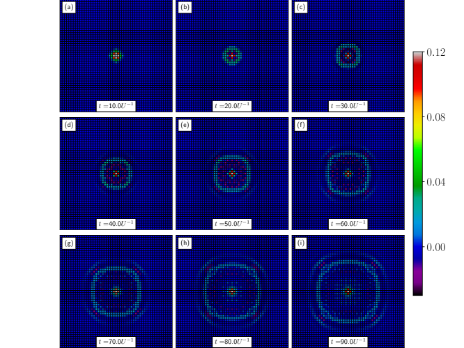
Figure 6: (Color online) (a)-(i) Spatial dependency of $\rho_{1}\left(\Delta\vec{r},t\right)$ at different moments in time $t/U^{-1}$ for a $50\times 50$ site system. The parameters are $\beta U=1000$, $\mu/U=0.4136$, $J_{f}/U=0.025$, $t_{c}/U^{-1}=5$, and $\tau_{Q}/U^{-1}=0.1$.

The spatial dependence of $\rho_{1}\left(\Delta\vec{r},t\right)$ at different moments in time for a $50\times 50$ site system is shown in Fig. 6, where each pixel represents a different particle separation displacement $\Delta\vec{r}/a$, and $\Delta\vec{r}/a=0$ is in the middle of each panel. From the figure, we see that the propagation of the single-particle correlations is anisotropic, with the propagation velocity being maximal along the diagonal and minimal along the crystal axes. Krutitsky et al. Krutitsky et al. (2014) found the same anisotropic spreading of single-particle correlations for the same quench protocol. Anisotropic behavior was also observed by Carleo et al. Carleo et al. (2014) in the spreading of density-density correlations within the superfluid regime. However, they found that the propagation velocity was maximal along the crystal axes and minimal along the diagonal, opposite to the behaviour observed here and in Ref. Krutitsky et al. (2014) for the Mott insulator.

We found acquiring estimates for the propagation velocities in higher dimensions to be somewhat more difficult than in one dimension. This difficulty is illustrated in Fig. 7 where we extract the propagation velocities along a crystal axis and the diagonal for the same $50\times 50$ system considered in Fig. 6. Figs. 5(a) and (b) display the time evolution of $\rho_{1}\left(\Delta\vec{r},t\right)$ for $\Delta\vec{r}/a=\left(8,0\right)$ (i.e. along a crystal axis) and $\Delta\vec{r}/a=\left(8,8\right)$ (i.e. along a diagonal) respectively. Upon comparing the two figures, we see that the wavepacket along the crystal axis is less sharp than that along the diagonal. Consequently, there is more uncertainy in our estimate of the center of a wavepacket (and hence the propagation velocity) along a crystal axis than along a diagonal. This trend extends to three dimensions as well where the wavepackets are sharpest along the main diagonals, less sharp along the secondary diagonals, and even less sharp along the crystal axes. The linear fits in Figs. 7(c) and (d) yield the following velocity estimates

$$v_{10}=\left(6.8\pm 0.3\right)\frac{J_{f}a}{\hbar},$$ (30)

$$v_{11}=\left(8.1\pm 0.1\right)\frac{J_{f}a}{\hbar},$$ (31)

where $v_{10}$ and $v_{11}$ are the propagation velocities along the crystal axes and the diagonals respectively.

Figures 8(a)-(c) plot the propagation velocities for a $50\times 50$ system as a function of $\mu/U$, $\beta U$, and $J_{f}/U$ respectively while keeping all the remaining parameters fixed. From Figs. 8(a) and (b), we see that the propagation velocities are not very sensitive to $\mu$, or to temperatures below the full melting of the Mott insulating phase ($\beta\gtrsim 5U$). In Fig. 8(c), we see that there appears to be a slight increase in propagation velocity and a decrease in anisotropy for larger $J_{f}/U$. Extrapolating to larger values of $J_{f}/U$ it seems plausible that there might be a value of $J_{f}/U$ where the spreading of correlations becomes isotropic, especially given the results of Carleo et al. Carleo et al. (2014) in the superfluid regime, where they found the maximal propagation velocity to be along the crystal axes, not the diagonals. In future work, we plan to investigate quench protocols where one crosses the phase boundary into the superfluid regime which will allow us to verify if this is indeed the case. Technically this requires the inclusion of broken symmetry terms in the equations of motion since these terms are required for a full description of the superfluid regime.

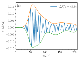
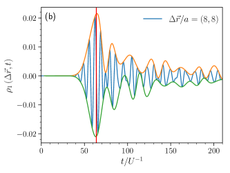
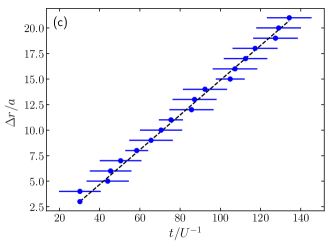
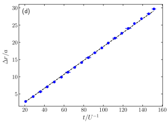
Figure 7: (Color online) Tracking the wavefront for a $50\times 50$ site system. (a) Dynamics of $\rho_{1}\left(\Delta\vec{r},t\right)$ for $\Delta\vec{r}/a=\left(8,0\right)$; (b) dynamics of $\rho_{1}\left(\Delta\vec{r},t\right)$ for $\Delta\vec{r}/a=\left(8,8\right)$; (c) scatter plot of the time $t/U^{-1}$ it takes for the single-particle correlation front to travel a distance $\Delta r/a$ along a crystal axis; (d) scatter plot of the time $t/U^{-1}$ it takes for the single-particle correlation front to travel a distance $\Delta r/a$ along a diagonal. We show a straight line fit to the data. In (b) and (c), the orange and green lines trace the envelopes of the wavepackets while the red line estimates the position of the centre of the first wavepacket. The parameters for (a)-(d) are $\mu/U=0.4116$, $\beta U=1000$, $J_{f}/U=0.025$, $t_{c}/U^{-1}=5$, and $\tau_{Q}/U^{-1}=0.1$.

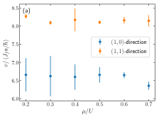
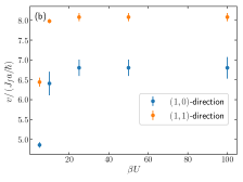
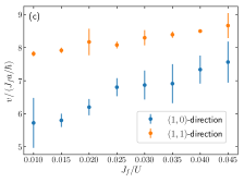
Figure 8: (Color online) Scatter plots of the propagation velocity $v/\left(J_{f}a/\hbar\right)$ in two dimension for a 50$\times$50 site system as a function of various model parameters. In all cases $t_{c}/U^{-1}=5$, and $\tau_{Q}/U^{-1}=0.1$. (a) scatter plot of $v/\left(J_{f}a/\hbar\right)$ as a function of $J_{f}/U$ with $\beta U=1000$, and $\mu/U=0.4136$; (b) scatter plot of $v/\left(J_{f}a/\hbar\right)$ as a function of $\beta U$ with $\mu/U=0.4136$ and $J_{f}/U=0.025$; (c) Scatter plot of $v/\left(J_{f}a/\hbar\right)$ as a function of $J_{f}/U$ with $\beta U=1000$, and $\mu/U=0.4136$.

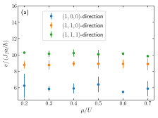
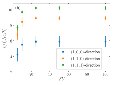
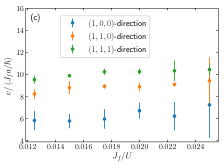
Figure 9: (Color online) Scatter plots of the propagation velocity $v/\left(J_{f}a/\hbar\right)$ in three dimension for a 28$\times$28 site system as a function of various model parameters. In all cases $t_{c}/U^{-1}=5$, and $\tau_{Q}/U^{-1}=0.1$. (a) scatter plot of $v/\left(J_{f}a/\hbar\right)$ as a function of $J_{f}/U$ with $\beta U=1000$, and $\mu/U=0.4132$; (b) scatter plot of $v/\left(J_{f}a/\hbar\right)$ as a function of $\beta U$ with $\mu/U=0.4132$ and $J_{f}/U=0.0175$; (c) Scatter plot of $v/\left(J_{f}a/\hbar\right)$ as a function of $J_{f}/U$ with $\beta U=1000$, and $\mu/U=0.4132$.

In 2 dimensions, the velocities $v_{10}$ we obtained along the crystal axes ranged from $5.7\text{--}7.6\,Ja/\hbar$ whereas the velocities $v_{11}$ along the diagonal ranged from $7.8\text{--}8.7\,Ja/\hbar$. The only other related study that we are aware of is that of Krutitsky et al. Krutitsky et al. (2014), where they obtained analytical estimates of $v_{10}=3Ja/\hbar$ and $v_{11}=3\sqrt{2}Ja/\hbar$ for the crystal axes and diagonals respectivekly. It is worth pointing out that Krutitsky et al. also performed numerical calculations of the single-particle correlation spreading beyond their lowest order analytical calculations, however they did not report any velocity estimates based on their numerical data. One prediction of Krutitsky et al. that does seem reasonably robust is the ratio $v_{11}/v_{10}$, for which their lowest order estimate is $\sqrt{2}$. Examination of Fig. 8(c) shows that our results are consistent with $v_{11}/v_{10}\simeq\sqrt{2}$ for small $J_{f}/U$, with the ratio decreasing with increasing $J_{f}/U$.

IV.2.3 3 dimensions

We see similar behaviour in three dimensions compared to that in two dimensions, as displayed in Fig. 9 where we see that the velocity depends strongly on crystal direction but is otherwise relatively insensitive to changes in chemical potential, temperature or final hopping value $J_{f}$. The trend towards increasing isotropy in the spread of correlations as $J_{f}/U$ increases is much less pronounced than in two dimensions, perhaps because we consider smaller values of $J_{f}$ than in two dimensions. To the best of our knowledge, our work is the first to calculate propagation velocities for correlations in three dimensions for the BHM, and we find that $v_{100}\sim 6\,J_{f}a/\hbar$, $v_{110}\sim 8.5\,J_{f}a/\hbar$ and $v_{111}\sim 10\,J_{f}a/\hbar$.

V Discussion and conclusions

The ability to address single sites in cold atom experiments (Bakr et al., 2010) has allowed for experimental exploration of spatio-temporal correlations in the BHM (Cheneau et al., 2012). This has led to theoretical investigations of these correlations in both one (Barmettler et al., 2012) and higher dimensions (Carleo et al., 2014; Natu and Mueller, 2013; Yanay and Mueller, 2016; Krutitsky et al., 2014) in the presence of a quench. In dimensions higher than one, where numerical approaches are limited, a theoretical challenge has been to develop a framework which can treat correlations in both the superfluid and Mott insulating phases over the course of a quench. In a previous paper (Fitzpatrick and Kennett, 2018), we developed a formalism that allows for such a description of the space and time dependence of single-particle correlations. The specific approach we took was to derive a 2PI effective action for the BHM using the KP contour, building on the 1PI real-time strong-coupling low-energy theory developed in Ref. (Kennett and Dalidovich, 2011) which generalized the imaginary-time theory developed in Ref. (Sengupta and Dupuis, 2005). From this 2PI effective action we were able to derive equations of motion that treat the superfluid order parameter and the full two-point Green’s functions on equal footing. One of the attractive features of the formalism is that it is applicable even in the limit of low occupation number per site.

Here, we used the formalism to study out of equilibrium dynamics, focusing on the light-cone like spreading of single-particle correlations after a quench. We considered quenches in the Mott insulator phase and solved the equations of motion for the single-particle density matrix $\rho_{1}\left(\Delta\vec{r},t\right)$. From the calculation of $\rho_{1}\left(\Delta\vec{r},t\right)$, we demonstrated light-cone like spreading of single-particle correlations in one, two and three dimensions. The range of propagation velocities that we obtain in one dimension over the range of parameter values we consider agree well with recent theoretical Barmettler et al. (2012) and experimental results Cheneau et al. (2012). Interestingly, it seems that the results we obtain for single-particle correlations appear to be similar to those obtained for density-density correlations. In higher dimensions, we find that there is an anisotropic spreading of correlations, where the propagation velocity is maximal along the main diagonal and minimal along crystal axes. Similar anisotropic spreading of correlations was observed in Ref. Krutitsky et al. (2014). We also observed that at least in two dimensions, the degree of anisotropy appears to diminish with increasing final hopping strength $J_{f}$. This raises the question of whether the spreading becomes isotropic for $J_{f}$ in the vicinity of $J_{c}$, particularly given that there has been the prediction that in the superfluid regime the propagation velocity is maximal along the crystal axes, rather than the diagonals Carleo et al. (2014). To address these questions within our formalism requires a more careful treatment of the equations of motion. One needs to include broken symmetry terms which become relevant upon entering the superfluid regime. We defer this task to future work.

The space and time dependence of correlations after a quantum quench give insight into the propagation of excitations generated by that quench, and hence we hope that the formalism we have developed here will allow further theoretical investigation of the excitations after quenches in the BHM, to complement experimental efforts in the same direction. In future work we plan to investigate a broader range of quench protocols, and generalizations such as the inclusion of a harmonic trap, coupling to a bath (Robertson et al., 2011; Dalidovich and Kennett, 2009; Guo et al., 2018), disorder (White et al., 2009; Pasienski et al., 2010; Choi et al., 2016; Meldgin et al., 2016), or multicomponent (Rubio-Abadal et al., 2018) Bose Hubbard models.

Appendix A Numerical implementation of solution of equations of motion

In this Appendix, we describe in more detail the numerical implementation of the solutions to the equations of motion. We begin by rewriting Eqs. (15) and (16) in a slightly more compact form:

$$A_{\vec{k}}\left(t,t^{\prime}\right) =\mathcal{A}\left(t-t^{\prime}\right)$$

$$\quad+\int_{t^{\prime}}^{t}dt^{\prime\prime}K_{\vec{k}}^{\left(1\right)}\left(t,t^{\prime\prime},n\left(t^{\prime\prime}\right)\right)A_{\vec{k}}\left(t^{\prime\prime},t^{\prime}\right),$$ (32)

$$G_{\vec{k}}^{\left(K\right)}\left(t,t^{\prime}\right) =\mathcal{G}^{\left(K\right)}\left(t-t^{\prime}\right)$$

$$\quad+\int_{0}^{t}dt^{\prime\prime}K_{\vec{k}}^{\left(1\right)}\left(t,t^{\prime\prime},n\left(t^{\prime\prime}\right)\right)G_{\vec{k}}^{\left(K\right)}\left(t^{\prime\prime},t^{\prime}\right)$$

$$\quad+\int_{0}^{t^{\prime}}dt^{\prime\prime}K_{\vec{k}}^{\left(2\right)}\left(t,t^{\prime\prime},n\left(t^{\prime\prime}\right)\right)A_{\vec{k}}\left(t^{\prime\prime},t^{\prime}\right),$$ (33)

where we define the kernels

$$K_{\vec{k}}^{\left(1\right)}\left(t,t^{\prime\prime},n\left(t^{\prime\prime}\right)\right) =-i\mathcal{A}\left(t-t^{\prime\prime}\right)\Sigma_{\vec{k}}^{\left(HFB\right)}\left(t^{\prime\prime}\right),$$ (34)

$$K_{\vec{k}}^{\left(2\right)}\left(t,t^{\prime\prime},n\left(t^{\prime\prime}\right)\right) =i\mathcal{G}^{\left(K\right)}\left(t-t^{\prime\prime}\right)\Sigma_{\vec{k}}^{\left(HFB\right)}\left(t^{\prime\prime}\right).$$ (35)

We include $n\left(t^{\prime\prime}\right)$ in the kernel arguments to emphasize the fact that both kernels are functions of the particle density. The presence of $n\left(t^{\prime\prime}\right)$ in the kernels couples the equations of motion for fixed quasi-momentum $\vec{k}$ to the remaining equations (with different $\vec{k}$) since $n\left(t^{\prime\prime}\right)$ is calculated from $\sum_{\vec{k}}G_{\vec{k}}^{\left(K\right)}\left(t^{\prime\prime},t^{\prime\prime}\right)$. Moreover, for $t\geq t^{\prime}$, the calculation of $A_{\vec{k}}\left(t,t^{\prime}\right)$ and $G_{\vec{k}}^{\left(K\right)}\left(t,t^{\prime}\right)$ depends on $n\left(t\right)$, not simply the history. These nonlinearities complicate the numerical solution as we must resort to implicit methods. At a general level, the simplest method to solve such a nonlinear system is to apply a self-consistent approach, which we do in this paper. For each timestep in $t$, we start by guessing the value of $n\left(t\right)$, then we solve each equation separately for values of $t^{\prime}$ in the range $t\geq t^{\prime}\geq 0$ using an explicit numerical approach, then we use our calculation of the $G_{\vec{k}}^{\left(K\right)}\left(t,t\right)$’s to update $n\left(t\right)$, and then we repeat until we obtain convergence. Once convergence is achieved, we take another timestep in $t$, then repeating the above procedure starting with $t^{\prime}=0$ to $t^{\prime}=t$. One can guess $n\left(t\right)$ using the final value for $n\left(t-\Delta t\right)$ or by doing an extrapolation based on several previous timesteps.

After guessing/updating the value of $n\left(t\right)$, we implement a modified block-by-block algorithm based on that in Ref. (Katani and Shahmorad, 2010). The block-by-block method uses a combination of Simpson’s rule and Lagrange interpolation points to discretize the equations of motion in such a way to generate a system of equations in terms of multiple unknowns that can then be solved simultaneously. For example, if we introduce the following discretization notation

$$F_{m}=F\left(m\Delta t\right),$$ (36)

then for fixed $m\geq m^{\prime}$, after applying the block-by-block procedure, we obtain a pair of simultaneous equations for $\left[A_{\vec{k}}\right]_{2m+1,2m^{\prime}}$ and $\left[A_{\vec{k}}\right]_{2m+2,2m^{\prime}}$, a single equation for $\left[A_{\vec{k}}\right]_{2m+1,2m^{\prime}+1}$, $\left[A_{\vec{k}}\right]_{2m+2,2m^{\prime}+1}$ and $\left[A_{\vec{k}}\right]_{2m+2,2m^{\prime}+2}$ each, a pair of simultaneous equations for $\left[G_{\vec{k}}^{\left(K\right)}\right]_{2m+1,2m^{\prime}}$ and $\left[G_{\vec{k}}^{\left(K\right)}\right]_{2m+2,2m^{\prime}}$, a pair of simultaneous equations for $\left[G_{\vec{k}}^{\left(K\right)}\right]_{2m+1,2m^{\prime}+1}$ and $\left[G_{\vec{k}}^{\left(K\right)}\right]_{2m+2,2m^{\prime}+1}$, and finally a single equation for $\left[G_{\vec{k}}^{\left(K\right)}\right]_{2m+2,2m^{\prime}+2}$. These “block” equations should be solved in the order as is written above since each block equation depends on the solutions to the block equations previous to it.

In summary, our numerical solution can be outlined as follows:

1. Set $m=0$.

2. Guess values for $n_{2m+1}$ and $n_{2m+2}$.

3. For each $\vec{k}$:

   1. For $m^{\prime}=0,\ldots,m$: Solve block equations.

4. Update $n_{2m+1}$ and $n_{2m+2}$ from the new $\left[G_{\vec{k}}^{\left(K\right)}\right]_{2m+1,2m^{\prime}+1}$ and $\left[G_{\vec{k}}^{\left(K\right)}\right]_{2m+2,2m^{\prime}+2}$ using Eqs. (21) and (22).

5. Check convergence of $n_{2m+1}$ and $n_{2m+2}$: if achieved then set $m\to m+1$ and return to step 2, else return to step 3 without incrementing $m$.

The algorithm outlined above is accurate to fourth order in the timestep. This self-consistent approach is advantageous as one can execute the outer $\vec{k}$ for-loop in step 3 in parallel which is the most computationally intensive step of the algorithm. The main computational constraint comes from the time integrals, which require considerable processing and memory resources. If $d$ is the number of spatial dimensions, $L$ is the number of sites along a crystal axis, and $N_{t}$ is the number of timesteps, then the memory requirements scale like $\binom{d+\lfloor L/2\rfloor}{d}N_{t}^{2}$. The binomial coefficient appears as a result of lattice symmetries and the periodic boundary conditions. Previous nonequilibrium 2PI studies which integrated similar equations of motion did not keep all of the history of the memory kernels for large times, which was justified by the argument that the two-time correlator would damp at an exponential rate (Rey et al., 2004; Berges and Cox, 2001; Aarts and Berges, 2001; Aarts et al., 2002; Berges, 2002). We do not make this assumption since it does not always hold for the quench protocols we consider.

Appendix B Particle number conservation

In this appendix, we identify the terms in the equations of motion that break particle number conservation. We start with the Dyson’s equation [Eq. (14)] noting that the bare propagator $G_{0}$ in this context is the atomic propagator $\mathcal{G}$

$$G_{\vec{k}}^{a_{1}a_{2},c}\left(\tau_{1},\tau_{2}\right)\equiv\mathcal{G}^{a_{1}a_{2}}\left(\tau_{1},\tau_{2}\right)+\int_{C}\int_{C}d\tau_{3}d\tau_{4}\,\mathcal{G}^{a_{1}a_{3}}\left(\tau_{1},\tau_{3}\right)\Sigma_{\vec{k}}^{\overline{a_{3}}\overline{a_{4}}}\left(\tau_{3},\tau_{4}\right)G_{\vec{k}}^{a_{4}a_{2},c}\left(\tau_{4},\tau_{2}\right).$$ (37)

Next, we act on both sides with $\delta\left(\tau_{1}^{\prime},\tau_{1}\right)\left\{i\partial_{\tau_{1}}-E_{\vec{k}}\right\}$, where for the moment, $E_{\vec{k}}$ is an unspecified function of $\vec{k}$. We then integrate over $\tau_{1}$, and set $\left(\tau_{1}^{\prime},\tau_{2}\right)=\left(\tau,\tau^{+}\right)$ and $\left(a_{1},a_{2}\right)=\left(1,2\right)$ to get

$$i\frac{\partial}{\partial\tau_{1}}G_{\vec{k}}^{12,c}\left(\tau_{1}=\tau,\tau_{2}=\tau^{+}\right) \equiv E_{\vec{k}}G_{\vec{k}}^{12,c}\left(\tau_{1}=\tau,\tau_{2}=\tau^{+}\right)+\left\{i\frac{\partial}{\partial\tau_{1}}-E_{\vec{k}}\right\}\mathcal{G}^{12}\left(\tau_{1}=\tau,\tau_{2}=\tau^{+}\right)$$

$$\quad+\int_{C}\int_{C}d\tau_{3}d\tau_{4}\left\{i\frac{\partial}{\partial\tau_{1}}-E_{\vec{k}}\right\}\mathcal{G}^{12}\left(\tau_{1}=\tau,\tau_{3}\right)\Sigma_{\vec{k}}^{1\overline{a}}\left(\tau_{3},\tau_{4}\right)G_{\vec{k}}^{a2,c}\left(\tau_{4},\tau_{2}=\tau^{+}\right).$$ (38)

The general form of the contour-time derivative of $G_{\vec{k}}^{12,c}$ is

$$\frac{\partial}{\partial\tau_{1}}G_{\vec{k}}^{12,c}\left(\tau_{1},\tau_{2}\right) =-i\frac{\partial}{\partial\tau_{1}}\left\{\Theta\left(\tau_{1},\tau_{2}\right)\left\langle\hat{a}_{\vec{k}}\left(\tau_{1}\right)\hat{a}_{\vec{k}}^{\dagger}\left(\tau_{2}\right)\right\rangle_{\hat{\rho}_{i}}^{c}+\Theta\left(\tau_{2},\tau_{1}\right)\left\langle\hat{a}_{\vec{k}}^{\dagger}\left(\tau_{2}\right)\hat{a}_{\vec{k}}\left(\tau_{1}\right)\right\rangle_{\hat{\rho}_{i}}^{c}\right\}$$

$$=-i\delta\left(\tau_{1},\tau_{2}\right)-i\Theta\left(\tau_{1},\tau_{2}\right)\frac{\partial}{\partial\tau_{1}}\left\langle\hat{a}_{\vec{k}}\left(\tau_{1}\right)\hat{a}_{\vec{k}}^{\dagger}\left(\tau_{2}\right)\right\rangle_{\hat{\rho}_{i}}^{c}$$

$$\quad-i\Theta\left(\tau_{2},\tau_{1}\right)\frac{\partial}{\partial\tau_{1}}\left\langle\hat{a}_{\vec{k}}^{\dagger}\left(\tau_{2}\right)\hat{a}_{\vec{k}}\left(\tau_{1}\right)\right\rangle_{\hat{\rho}_{i}}^{c},$$ (39)

which also applies to $\mathcal{G}^{12}$.

The Dyson’s equation can also be rewritten as follows

$$G_{\vec{k}}^{a_{1}a_{2},c}\left(\tau_{1},\tau_{2}\right)\equiv\mathcal{G}^{a_{1}a_{2}}\left(\tau_{1},\tau_{2}\right)+\int_{C}\int_{C}d\tau_{3}d\tau_{4}G_{\vec{k}}^{a_{1}a_{3},c}\left(\tau_{1},\tau_{3}\right)\Sigma_{\vec{k}}^{\overline{a_{3}}\overline{a_{4}}}\left(\tau_{3},\tau_{4}\right)\mathcal{G}^{a_{4}a_{2}}\left(\tau_{4},\tau_{2}\right).$$ (40)

We again act on both sides with $\delta\left(\tau_{2}^{\prime},\tau_{2}\right)\left\{i\partial_{\tau_{2}}+E_{\vec{k}}\right\}$, integrate over $\tau_{2}$, and set $\left(\tau_{1},\tau_{2}\right)=\left(\tau,\tau^{+}\right)$, $\left(a_{1},a_{2}\right)=\left(1,2\right)$ to get

$$i\frac{\partial}{\partial\tau_{2}}G_{\vec{k}}^{12,c}\left(\tau_{1}=\tau,\tau_{2}=\tau^{+}\right) \equiv-E_{\vec{k}}G_{\vec{k}}^{12,c}\left(\tau_{1}=\tau,\tau_{2}=\tau^{+}\right)+\left\{i\partial_{\tau_{2}}+E_{\vec{k}}\right\}\mathcal{G}^{12}\left(\tau_{1}=\tau,\tau_{2}=\tau^{+}\right)$$

$$\quad+\int_{C}\int_{C}d\tau_{3}d\tau_{4}G_{\vec{k}}^{1a,c}\left(\tau_{1},\tau_{3}\right)\Sigma_{\vec{k}}^{\overline{a}2}\left(\tau_{3},\tau_{4}\right)\left\{i\partial_{\tau_{2}}+E_{\vec{k}}\right\}\mathcal{G}^{12,c}\left(\tau_{4},\tau_{2}=\tau^{+}\right).$$ (41)

Similarly to Eq. (39), we obtain

$$\frac{\partial}{\partial\tau_{2}}G_{\vec{k}}^{12,c}\left(\tau_{1},\tau_{2}\right) =i\delta\left(\tau_{1},\tau_{2}\right)-i\Theta\left(\tau_{1},\tau_{2}\right)\frac{\partial}{\partial\tau_{2}}\left\langle\hat{a}_{\vec{k}}\left(\tau_{1}\right)\hat{a}_{\vec{k}}^{\dagger}\left(\tau_{2}\right)\right\rangle_{\hat{\rho}_{i}}^{c}$$

$$\quad-i\Theta\left(\tau_{2},\tau_{1}\right)\frac{\partial}{\partial\tau_{2}}\left\langle\hat{a}_{\vec{k}}^{\dagger}\left(\tau_{2}\right)\hat{a}_{\vec{k}}\left(\tau_{1}\right)\right\rangle_{\hat{\rho}_{i}}^{c}.$$ (42)

It then follows from Eqs. (39) and (42) that

$$\frac{\partial}{\partial\tau_{1}}G_{\vec{k}}^{12,c}\left(\tau_{1}=\tau,\tau_{2}=\tau^{+}\right)+\frac{\partial}{\partial\tau_{2}}G_{\vec{k}}^{12,c}\left(\tau_{1}=\tau,\tau_{2}=\tau^{+}\right)=-i\frac{d}{d\tau_{1}}n_{\vec{k}}\left(\tau_{1}=\tau\right).$$ (43)

Note that in the special case where $G_{\vec{k}}^{12,c}=\mathcal{G}^{12}$, one can show explicitly from the analytical expressions for $\mathcal{G}^{12}$ [see Appendix C of Ref. (Fitzpatrick and Kennett, 2018)] that the right-hand-side of Eq. (43) vanishes.

Next, by adding Eqs. (38) and (41) together, summing over all $\vec{k}$, and using Eqs. (39), (42), and (43), we get

$$\frac{d}{d\tau_{1}}\left\{N\left(\tau_{1}=\tau\right)\right\} =\sum_{\vec{k}}\int_{C}\int_{C}d\tau_{3}d\tau_{4}\left\{i\frac{\partial}{\partial\tau_{1}}-E_{\vec{k}}\right\}\mathcal{G}^{12}\left(\tau_{1}=\tau,\tau_{3}\right)\Sigma_{\vec{k}}^{1\overline{a}}\left(\tau_{3},\tau_{4}\right)G_{\vec{k}}^{a2,c}\left(\tau_{4},\tau_{2}=\tau^{+}\right)$$

$$\quad+\sum_{\vec{k}}\int_{C}\int_{C}d\tau_{3}d\tau_{4}G_{\vec{k}}^{1a,c}\left(\tau_{1},\tau_{3}\right)\Sigma_{\vec{k}}^{\overline{a}2}\left(\tau_{3},\tau_{4}\right)\left\{i\partial_{\tau_{2}}+E_{\vec{k}}\right\}\mathcal{G}^{12}\left(\tau_{4},\tau_{2}=\tau^{+}\right).$$ (44)

Now, if we set $E_{\vec{k}}=\epsilon_{\vec{k}}-\mu$ (i.e we set $E_{\vec{k}}$ to the single-particle excitation energy of a free particle), and replace $\mathcal{G}^{12}$ by the free propagator for the BHM obtained when $U=0$, then

$$\left\{i\frac{\partial}{\partial\tau_{1}}-E_{\vec{k}}\right\}\mathcal{G}^{12}\left(\tau_{1}=\tau,\tau_{3}\right) \to\delta\left(\tau,\tau_{3}\right),$$ (45)

$$\left\{i\frac{\partial}{\partial\tau_{2}}+E_{\vec{k}}\right\}\mathcal{G}^{12,c}\left(\tau_{4},\tau_{2}=\tau^{+}\right) \to-\delta\left(\tau_{4},\tau^{\prime}\right),$$ (46)

and Eq. (44) would become

$$\frac{d}{d\tau_{1}}N\left(\tau_{1}=\tau\right)=\sum_{\vec{k}}\int_{C}d\tau_{3}\left\{\Sigma_{\vec{k}}^{1\overline{a}}\left(\tau,\tau_{3}\right)G_{\vec{k}}^{a2,c}\left(\tau_{3},\tau^{+}\right)-G_{\vec{k}}^{1a}\left(\tau,\tau_{3}\right)\Sigma_{\vec{k}}^{\overline{a}2}\left(\tau_{3},\tau^{+}\right)\right\}.$$ (47)

Baym showed that the term on the right-hand-side of Eq. (47) vanishes as long as the self-energy $\Sigma$ is of the form $\delta\Phi/\delta G$, with $\Phi$ a functional of $G$ (Baym, 1962; Stefanucci and van Leeuwen, 2013). As we mentioned in Sec. III, we obtained our self-energy by taking a functional derivative of the 2PI effective action, which is indeed a functional of $G$, hence the right-hand-side of Eq. (47) vanishes and the particle number is conserved. It is worth stressing that in this scenario, the self-energy need not be calculated to all orders so that particle number is conserved. As long as the approximation of the self-energy is of the form $\delta\Phi/\delta G$, even after taking some low-energy approximation as we do in our effective theory, conservation will still be guaranteed.

In our case, $\mathcal{G}^{12}$ is not the free propagator for the BHM obtained when $U=0$, but instead is the atomic propagator obtained in the limit when $J=0$. Hence there exists no function $E_{\vec{k}}$ in which Eqs. (45) and (46) could be possibly satisfied. The reason for this is due to the asymmetry between the single-particle and hole excitation energies. For the free propagator, $E^{\left(+\right)}=-E^{\left(-\right)}$, where $E^{\left(+\right)}$ and $E^{\left(-\right)}$ are the single-particle and hole excitation energies respectively, whereas for the atomic propagator $\mathcal{G}^{12}$, $E^{\left(+\right)}\neq-E^{\left(-\right)}$ for all values of $\mu$. Due to this asymmetry, additional terms are generated leading to

$$\frac{d}{d\tau_{1}}N\left(\tau_{1}=\tau\right) =i\sum_{\vec{k}}\int_{C}\int_{C}d\tau_{3}d\tau_{4}\left[\partial_{\tau_{1}}\mathcal{G}^{12}\right]\left(\tau_{1}=\tau,\tau_{3}\right)\Sigma_{\vec{k}}^{1\overline{a}}\left(\tau_{3},\tau_{4}\right)G_{\vec{k}}^{a2,c}\left(\tau_{4},\tau_{2}=\tau^{+}\right)$$

$$\quad+i\sum_{\vec{k}}\int_{C}\int_{C}d\tau_{3}d\tau_{4}G_{\vec{k}}^{1a,c}\left(\tau_{1},\tau_{3}\right)\Sigma_{\vec{k}}^{\overline{a}2}\left(\tau_{3},\tau_{4}\right)\left[\partial_{\tau_{2}}\mathcal{G}^{12}\right]\left(\tau_{4},\tau_{2}=\tau^{+}\right),$$ (48)

where we introduce the following shorthand notation:

$$\left[\partial_{\tau_{1}}\right]G_{\vec{k}}^{12,c}\left(\tau_{1},\tau_{2}\right) =-i\Theta\left(\tau_{1},\tau_{2}\right)\frac{\partial}{\partial\tau_{1}}\left\langle\hat{a}_{\vec{k}}\left(\tau_{1}\right)\hat{a}_{\vec{k}}^{\dagger}\left(\tau_{2}\right)\right\rangle_{\hat{\rho}_{i}}^{c}-i\Theta\left(\tau_{2},\tau_{1}\right)\frac{\partial}{\partial\tau_{1}}\left\langle\hat{a}_{\vec{k}}^{\dagger}\left(\tau_{2}\right)\hat{a}_{\vec{k}}\left(\tau_{1}\right)\right\rangle_{\hat{\rho}_{i}}^{c},$$ (49)

$$\left[\partial_{\tau_{2}}\right]G_{\vec{k}}^{12,c}\left(\tau_{1},\tau_{2}\right) =-i\Theta\left(\tau_{1},\tau_{2}\right)\frac{\partial}{\partial\tau_{2}}\left\langle\hat{a}_{\vec{k}}\left(\tau_{1}\right)\hat{a}_{\vec{k}}^{\dagger}\left(\tau_{2}\right)\right\rangle_{\hat{\rho}_{i}}^{c}-i\Theta\left(\tau_{2},\tau_{1}\right)\frac{\partial}{\partial\tau_{2}}\left\langle\hat{a}_{\vec{k}}^{\dagger}\left(\tau_{2}\right)\hat{a}_{\vec{k}}\left(\tau_{1}\right)\right\rangle_{\hat{\rho}_{i}}^{c},$$ (50)

where we now set $E_{\vec{k}}\to 0$ as it serves no purpose for us anymore. The terms on the right-hand-side of (48) are in general not zero. If we kept all terms in the effective theory and did not make the low energy approximation then the the right-hand-side of (48) should equal zero. However, because the bare propagator we use is the atomic propagator Baym’s arguments do not hold in the low energy theory and there is not conservation of particle number.

References

- Bloch (2005) I. Bloch, Nature Phys. 1, 23 (2005).
- Jaksch and Zoller (2005) D. Jaksch and P. Zoller, Ann. Phys. 315, 52 (2005).
- Morsch and Oberthaler (2006) O. Morsch and M. Oberthaler, Rev. Mod. Phys. 78, 179 (2006).
- Lewenstein et al. (2007) M. Lewenstein, A. Sanpera, V. Ahufinger, B. Damski, A. Sen, and U. Sen, Adv. Phys. 56, 243 (2007).
- Bloch et al. (2008) I. Bloch, J. Dalibard, and W. Zwerger, Rev. Mod. Phys. 80, 885 (2008).
- Kennett (2013) M. P. Kennett, ISRN Condensed Matter Physics 2013, 393616 (2013).
- Jaksch et al. (1998) D. Jaksch, C. Bruder, J. I. Cirac, C. W. Gardiner, and P. Zoller, Phys. Rev. Lett. 81, 3108 (1998).
- Fisher et al. (1989) M. P. A. Fisher, P. B. Weichman, G. Grinstein, and D. S. Fisher, Phys. Rev. B 40, 546 (1989).
- Greiner et al. (2002) M. Greiner, O. Mandel, T. Esslinger, T. W. Hänsch, and I. Bloch, Nature 415, 39 (2002).
- Chen et al. (2011) D. Chen, M. White, C. Borries, and B. DeMarco, Phys. Rev. Lett. 106, 235304 (2011).
- Hung et al. (2010) C.-L. Hung, X. Zhang, N. Gemelke, and C. Chin, Phys. Rev. Lett. 104, 160403 (2010).
- Bakr et al. (2010) W. S. Bakr, A. Peng, M. E. Tai, R. Ma, J. Simon, J. I. Gillen, S. Fölling, L. Pollet, and M. Greiner, Science 329, 547 (2010).
- Kibble (1976) T. W. B. Kibble, J. Phys. A 9, 1387 (1976).
- Zurek (1985) W. H. Zurek, Nature 317, 505 (1985).
- Zurek et al. (2005) W. H. Zurek, U. Dorner, and P. Zoller, Phys. Rev. Lett. 95, 105701 (2005).
- Clark and Jaksch (2004) S. R. Clark and D. Jaksch, Phys. Rev. A 70, 043612 (2004).
- Kollath et al. (2007) C. Kollath, A. M. Läuchli, and E. Altman, Phys. Rev. Lett. 98, 180601 (2007).
- Sciolla and Biroli (2010) B. Sciolla and G. Biroli, Phys. Rev. Lett. 105, 220401 (2010).
- Sciolla and Biroli (2011) B. Sciolla and G. Biroli, J. Stat. Mech. 11, 11003 (2011).
- Fischer et al. (2008) U. R. Fischer, R. Schützhold, and M. Uhlmann, Phys. Rev. A 77, 043615 (2008).
- Fischer and Schützhold (2008) U. R. Fischer and R. Schützhold, Phys. Rev. A 78, 061603 (2008).
- Kennett and Dalidovich (2011) M. P. Kennett and D. Dalidovich, Phys. Rev. A 84, 033620 (2011).
- Strand et al. (2015) H. U. R. Strand, M. Eckstein, and P. Werner, Physical Review X 5, 011038 (2015).
- Landea and Nessi (2015) I. S. Landea and N. Nessi, Phys. Rev. A 91, 063601 (2015).
- Polkovnikov (2005) A. Polkovnikov, Phys. Rev. B 72, 161201 (2005).
- Natu et al. (2011) S. S. Natu, K. R. A. Hazzard, and E. J. Mueller, Phys. Rev. Lett. 106, 125301 (2011).
- Bernier et al. (2011) J.-S. Bernier, G. Roux, and C. Kollath, Phys. Rev. Lett. 106, 200601 (2011).
- Natu and Mueller (2013) S. S. Natu and E. J. Mueller, Phys. Rev. A 87, 063616 (2013).
- Bernier et al. (2012) J.-S. Bernier, D. Poletti, P. Barmettler, G. Roux, and C. Kollath, Phys. Rev. A 85, 033641 (2012).
- Zakrzewski (2005) J. Zakrzewski, Phys. Rev. A 71, 043601 (2005).
- Trefzger and Sengupta (2011) C. Trefzger and K. Sengupta, Phys. Rev. Lett. 106, 095702 (2011).
- Yanay and Mueller (2016) Y. Yanay and E. J. Mueller, Phys. Rev. A 93, 013622 (2016).
- Lieb and Robinson (1972) E. H. Lieb and D. W. Robinson, Commun. Math. Phys. 28, 251 (1972).
- Carleo et al. (2014) G. Carleo, F. Becca, L. Sanchez-Palencia, S. Sorella, and M. Fabrizio, Phys. Rev. A. 89, 031602 (2014).
- Läuchli and Kollath (2008) A. M. Läuchli and C. Kollath, J. Stat. Mech. 5, 05018 (2008).
- Barmettler et al. (2012) P. Barmettler, D. Poletti, M. Cheneau, and C. Kollath, Phys. Rev. A 85, 053625 (2012).
- Krutitsky et al. (2014) K. V. Krutitsky, P. Navez, F. Queisser, and R. Schützhold, Eur. Phys. J. Quant. Tech. 1 (2014).
- Cheneau et al. (2012) M. Cheneau, P. Barmettler, D. Poletti, M. Endres, P. Schauß, T. Fukuhara, C. Gross, I. Bloch, C. Kollath, and S. Kuhr, Nature 481, 484 (2012).
- Navez and Schützhold (2010) P. Navez and R. Schützhold, Phys. Rev. A 82, 063603 (2010).
- Trotzky et al. (2012) S. Trotzky, Y.-A. Chen, A. Flesch, I. P. McCulloch, U. Schollwöck, J. Eisert, and I. Bloch, Nature Phys. 8, 325 (2012).
- Amico and Penna (2000) L. Amico and V. Penna, Phys. Rev. B 62, 1224 (2000).
- Dutta et al. (2012) A. Dutta, C. Trefzger, and K. Sengupta, Phys. Rev. B 86, 085140 (2012).
- Schroll et al. (2004) C. Schroll, F. Marquardt, and C. Bruder, Phys. Rev. A 70, 053609 (2004).
- Queisser et al. (2014) F. Queisser, K. V. Krutitsky, P. Navez, and R. Schützhold, Phys. Rev. A 89, 033616 (2014).
- Fitzpatrick and Kennett (2018) M. R. C. Fitzpatrick and M. P. Kennett, Nuclear Physics B 930, 1 (2018).
- Sengupta and Dupuis (2005) K. Sengupta and N. Dupuis, Phys. Rev. A 71, 033629 (2005).
- Konstantinov and Perel (1961) O. V. Konstantinov and V. I. Perel, Sov. Phys. JETP 12, 142 (1961).
- Schwinger (1961) J. Schwinger, J. Math. Phys. 2, 407 (1961).
- Keldysh (1964) L. V. Keldysh, Zh. Eksp. Teor. Fiz. 20, 1515 (1964), [Sov. Phys. JETP 20, 1018 (1965)].
- Rammer and Smith (1986) J. Rammer and H. Smith, Rev. Mod. Phys. 58, 323 (1986).
- Niemi and Semenoff (1984) A. J. Niemi and G. W. Semenoff, Ann. Phys. 152, 105 (1984).
- Landsman and van Weert (1987) N. P. Landsman and C. G. van Weert, Phys. Rep. 145, 141 (1987).
- Chou et al. (1985) K.-c. Chou, Z.-b. Su, B.-l. Hao, and L. Yu, Phys. Rep. 118, 1 (1985).
- Robertson et al. (2011) A. Robertson, V. M. Galitski, and G. Refael, Phys. Rev. Lett. 106, 165701 (2011).
- Dalidovich and Kennett (2009) D. Dalidovich and M. P. Kennett, Phys. Rev. A 79, 053611 (2009).
- Graß et al. (2011a) T. D. Graß, F. E. A. dos Santos, and A. Pelster, Laser Phys. 21, 1459 (2011a).
- Graß et al. (2011b) T. D. Graß, F. E. A. Dos Santos, and A. Pelster, Phys. Rev. A 84, 013613 (2011b).
- Graß (2009) T. D. Graß, Real-time Ginzburg-Landau theory for bosonic gases in optical lattices, Master’s thesis, Freie Universität, Berlin (2009).
- Rey et al. (2004) A. M. Rey, B. L. Hu, E. Calzetta, A. Roura, and C. W. Clark, Phys. Rev. A 69, 033610 (2004).
- Rey et al. (2005) A. M. Rey, B. L. Hu, E. Calzetta, and C. W. Clark, Phys. Rev. A 72, 023604 (2005).
- Temme and Gasenzer (2006) K. Temme and T. Gasenzer, Phys. Rev. A 74, 053603 (2006).
- Calzetta et al. (2006) E. Calzetta, B. L. Hu, and A. M. Rey, Phys. Rev. A 73, 023610 (2006).
- Polkovnikov (2003) A. Polkovnikov, Phys. Rev. A 68, 053604 (2003).
- Lo Gullo and Dell’Anna (2016) N. Lo Gullo and L. Dell’Anna, Phys. Rev. B 94, 184308 (2016).
- Dupuis (2001) N. Dupuis, Nucl. Phys. B 618, 617 (2001).
- Sajna and Micnas (2018) A. S. Sajna and R. Micnas, Phys. Rev. A 97, 033605 (2018).
- Cornwall et al. (1974) J. M. Cornwall, R. Jackiw, and E. Tomboulis, Phys. Rev. D 10, 2428 (1974).
- Zwerger (2003) W. Zwerger, Journal of Optics B: Quantum and Semiclassical Optics 5, S9 (2003).
- Sen et al. (2008) D. Sen, K. Sengupta, and S. Mondal, Physical Review Letters 101, 016806 (2008).
- Katani and Shahmorad (2010) R. Katani and S. Shahmorad, Applied Mathematical Modelling 34, 400 (2010).
- Guo et al. (2018) C. Guo, I. de Vega, U. Schollwöck, and D. Poletti, Phys. Rev. A 97, 053610 (2018).
- White et al. (2009) M. White, M. Pasienski, D. Mckay, S. Q. Zhou, D. Ceperley, and B. DeMarco, Phys. Rev. Lett. 102, 055301 (2009).
- Pasienski et al. (2010) M. Pasienski, D. Mckay, M. White, and B. DeMarco, Nature Phys. 6, 677 (2010).
- Choi et al. (2016) J.-Y. Choi, S. Hild, J. Zeiher, P. Schauß, A. Rubio-Abadal, T. Yefsah, V. Khemani, D. A. Huse, I. Bloch, and C. Gross, Science 352, 1547 (2016).
- Meldgin et al. (2016) C. Meldgin, U. Ray, P. Russ, D. Chen, D. M. Ceperley, and B. DeMarco, Nature Phys. 12, 646 (2016).
- Rubio-Abadal et al. (2018) A. Rubio-Abadal, J.-Y. Choi, J. Zeiher, S. Hollerith, J. Rui, I. Bloch, and C. Gross, (2018), arXiv:1805.00056v1 .
- Berges and Cox (2001) J. Berges and J. Cox, Phys. Lett. B 517, 369 (2001).
- Aarts and Berges (2001) G. Aarts and J. Berges, Phys. Rev. D 64, 105010 (2001).
- Aarts et al. (2002) G. Aarts, D. Ahrensmeier, R. Baier, J. Berges, and J. Serreau, Phys. Rev. D 66, 045008 (2002).
- Berges (2002) J. Berges, Nucl. Phys. A 699, 847 (2002).
- Baym (1962) G. Baym, Phys. Rev. 127, 1391 (1962).
- Stefanucci and van Leeuwen (2013) G. Stefanucci and R. van Leeuwen, Nonequilibrium Many-Body Theory of Quantum Systems (Cambridge University Press, New York, NY, 2013).