Scale-invariance of parity-invariant three-dimensional QED
Abstract
We present numerical evidences using overlap fermions for a scale-invariant behavior of parity-invariant three-dimensional QED with two flavors of massless two-component fermions. Using finite-size scaling of the low-lying eigenvalues of the massless anti-Hermitian overlap Dirac operator, we rule out the presence of bilinear condensate and estimate the mass anomalous dimension. The eigenvectors associated with these low-lying eigenvalues suggest critical behavior in the sense of a metal-insulator transition. We show that there is no mass gap in the scalar and vector correlators in the infinite volume theory. The vector correlator does not acquire an anomalous dimension. The anomalous dimension associated with the long-distance behavior of the scalar correlator is consistent with the mass anomalous dimension.
pacs:
11.15.Ha, 11.10.Kk, 11.30.QcI Introduction
Two-component massless fermions coupled to a three-dimensional Euclidean abelian gauge field has been a topic of study in the past three decades for several field-theoretic reasons. The presence of parity anomaly Deser et al. (1982a, b); Redlich (1984); Niemi and Semenoff (1983) induces a topological mass term for the gauge fields. Soon after that, it found an application in condensed matter physics as a possible explanation of the quantum Hall effect Semenoff (1984). Recently, duality between various theories in three dimensions that includes fermions coupled to abelian gauge fields with or without Chern-Simons matter are being discussed in the context of condensed matter physics Seiberg et al. (2016); Karch and Tong (2016). Of particular interest to us in this paper is the possible conformal nature of parity-invariant theories with even number, , of massless flavors. This could have implications in the conductivity of graphene type materials Miransky and Shovkovy (2015); Castro Neto et al. (2009). Also, the theory seems to be of interest in the context of high- cuprates Franz et al. (2002); Herbut (2002).
A simple analysis of the associated gap equation Pisarski (1984) suggested that fermions could generate a mass as the number of flavors tends to infinity. Subsequent analysis of the gap equation Appelquist et al. (1985); Appelquist et al. (1986a, b); Appelquist et al. (1988) reached an opposite conclusion that the infra-red behavior of the large- theory is scale-invariant due to the presence of a non-trivial fixed point. However, it also lead to the possibility of a non-zero bilinear condensate if , and the conclusion remained stable when correction was included Kotikov et al. (2016). A computation of renormalization group flow including the presence of parity-invariant four-fermion terms, lead to a critical number of flavors in the region of to Braun et al. (2014). Comparing the free energies in the IR and UV assuming non-interacting particles, one finds that symmetry breaking is not expected when Appelquist et al. (1999); Appelquist and Wijewardhana (2004). Recently, there has been a renewed interest in parity-invariant QED3 due to the presence of Wilson-Fisher fixed point in dimensions. A similar comparison of the free energies, now assuming a conformal phase and a broken phase, suggests that symmetry is not broken when Giombi et al. (2015). A computation Giombi et al. (2016) of the coefficient of the two-point function of the stress energy tensor in the expansion supports a conformal phase if . Computations Di Pietro et al. (2016); Herbut (2016) of the scaling dimensions of the naively irrelevant four-fermion operators in the vicinity of the Wilson-Fisher fixed point suggest that the four-fermion operators become relevant for , and hence the possibility that the infra-red fixed point becomes unstable for . A computation Chester and Pufu (2016) of the scaling dimensions of the parity-even four-fermion operators in a expansion, taking into account the mixing with a larger basis of operators, suggests that theories with are conformal.
Earlier numerical work that studied the behavior of the fermion bilinear as a function of the fermion mass using staggered fermions Hands et al. (2002, 2004) indicated that there is evidence for a bilinear condensate for . The evidence for a condensate in was found to be weak. A numerical study Raviv et al. (2014) of the beta function for theory with Wilson fermions indicated that this is theory is not probably conformal 111We think that one can use the data presented in Table-II of Raviv et al. (2014) and reach a conclusion that theory has an IR fixed point. The value of physical size of the box, as defined in this paper, corresponding to the values of and in Raviv et al. (2014) is . A linear behavior can be seen in a plot of the inverse of the dimensionless renormalized coupling, , versus that includes their data from all . A non-zero intercept at seen in their data suggests the existence of the IR fixed point at .. A recent study Karthik and Narayanan (2016) of the spectrum of the low-lying eigenvalues of the massless Wilson-Dirac operator did not show any evidence for condensate for .
Of particular relevance is the U global symmetry formally present in the continuum fermion action
| (1) |
where are the two-component fermion fields. The U symmetry is broken to UU if one uses Wilson fermions as a regulator on the lattice, and it is only recovered in the continuum limit for massless fermions. Indeed, the numerical computations in Karthik and Narayanan (2016) were done such that the continuum limit was taken at a fixed physical volume and the infinite volume limit was subsequently studied. As we will show in this paper, the U symmetry is present at the lattice level if one uses overlap fermions. This is also the case if one regulates using domain wall fermions Hands (2016, 2015) and take the limit of infinite number of fermions in the extra direction.
Since the overlap formalism in odd dimensions Narayanan and Nishimura (1997); Kikukawa and Neuberger (1998) is not as well known as in even dimensions, we start with an introduction to overlap fermions in Section II. We point out the U symmetry present at the level of the generating functional for massless overlap fermions in a gauge field background. We perform numerical simulations using massless overlap fermions for the case of and extract continuum results in a periodic box of size, . Our aim is to show that the theory is scale-invariant. We explore three aspects of the theory to establish scale invariance:
-
1.
If the low-lying eigenvalues of the massless anti-Hermitian overlap operator depend on the finite physical size as
(2) with , then there is no bilinear condensate in the infinite volume theory and the exponent is the mass anomalous dimension. We will show that in Section IV. This is at the edge of the maximum allowed value for in a theory which is also conformally invariant Mack (1977).
-
2.
In the sense of a metal-insulator transition Osborn and Verbaarschot (1998); Al’tschuler and Shklovskii (1986); Al’tschuler et al. (1988); Chalker and Lerner (1996), we will show that the eigenvectors associated with the low lying eigenvalues lie in the critical regime. The inverse participation ratio (IPR) of the eigenvectors is defined as
(3) In the critical regime, the IPR would exhibit a scaling with the physical size as
(4) This scaling is related to the behavior of the number variance , the variance of the number of eigenvalues, , below a given value, . In the critical regime, would exhibit an asymptotic linear behavior with a slope :
(5) We will demonstrate in Section V that the low-lying eigensystem of the theory satisfy such a critical behavior with .
-
3.
We study the correlators of parity-even vector bilinear,
(6) and the scalar bilinear
(7) in Section VI. In both the cases, we will show there is no mass gap in their spectrum, and that the long-distance behavior of the correlators at zero spatial momentum exhibits a power-law. The power-law associated with the vector correlator does not acquire any anomalous dimension consistent with the vector bilinear being a conserved current. The scalar correlator does not show a simple power-law behavior as a function of Euclidean time, leading us to estimate the expected power-law at even longer distances inaccessible to our numerical simulation. The resulting value for the mass anomalous dimension is which is consistent with the result from the low lying eigenvalues and consistent with a vanishing correlator in the long distance limit.
II Overlap formalism in three dimensions
The overlap formalism for two-component fermions in three dimensions were originally discussed in Narayanan and Nishimura (1997); Kikukawa and Neuberger (1998) and more recently for parity-invariant four-component fermions by starting from domain wall fermions Hands (2016, 2015). In this paper, we start from the original overlap formalism Narayanan and Neuberger (1995) to obtain the result in three dimensions. In this manner, we will explicitly show the parity-invariant factorization into two two-component fermions.
II.1 Gauge-invariant but parity-breaking overlap operator for a single flavor of two-component massless fermion
The overlap formula Narayanan and Neuberger (1995) for a two-component fermion determinant in three dimensions is
| (8) |
where are the lowest states of the many body operators,
| (9) |
with and being two-component fermion creation and annihilation operators that obey canonical anti-commutation relations. The two single particle Hamiltonians are
| (10) |
The naïve massless Dirac operator in three dimensions is
| (11) |
with ; being the two-component Pauli matrices. The standard Wilson term is
| (12) |
with a Wilson mass parameter in the range .
The naïve massless Dirac operator in three dimensions is anti-Hermitian; . Due to this special structure of in Eq. (10), one can obtain an expression for in odd dimensions in terms of an explicit operator. Defining
| (13) |
we can set up the following eigenvalue problems:
| (14) |
It follows that
| (15) |
The basis of positive and negative eigenstates of are
| (16) |
respectively. On the one hand, the basis of positive and negative eigenstates of can be chosen to be
| (17) |
respectively and the fermion determinant for a single two-component fermion becomes
| (18) |
On the other hand, the basis of positive and negative eigenstates of can be chosen to be
| (19) |
respectively and the fermion determinant for a single two-component fermion becomes
| (20) |
In both cases, the fermion determinant is gauge invariant Kikukawa and Neuberger (1998). The phase of the fermion determinant arises from the phase of the Wilson-Dirac operator analyzed in detail in Karthik and Narayanan (2015) and carries the parity anomaly Narayanan and Nishimura (1997); Kikukawa and Neuberger (1998).
II.2 U symmetric parity and gauge-invariant overlap formalism
In order to realize a parity-invariant theory, we consider theories with even number of fermion flavors, . As shown in Appendix B, the result for the generating function for a theory, including parity invariant fermion masses and using flavor diagonal sources and , is
| (21) |
where
| (22) |
and
| (23) |
If we set , we observe that . Therefore, one has the full U symmetry in the fermionic sources. The fermion determinant in the absence of sources for the massless theory is
| (24) |
This also shows a U symmetry, but we have an additional factor of for each in the measure for the gauge fields, which is required to keep the theory parity invariant.
II.3 Eigenvalues of the overlap operator
The bilinear scalar condensate in a fixed gauge field background is given by
| (25) |
where are the eigenvalues of and is the density of eigenvalues obeying . Therefore, we are led to an analysis of the low-lying eigenvalues of in order to extract the mass anomalous dimension.
Given an eigenvalue of , the corresponding eigenvalue of is
| (26) |
Therefore, the low-lying eigenvalues come from values of close to . In order to obtain these numerically using the Ritz algorithm Kalkreuter and Simma (1996), we compute the low-lying eigenvalues of the positive definite operator,
| (27) |
The corresponding eigenvalue of this operator is . Due to parity invariance, we only need
| (28) |
III Set up of the numerical calculation
The numerical details essentially parallel the one used in our previous work Karthik and Narayanan (2016) with Wilson fermions. The only new ingredient is the presence of the operator defined in Eq. (15). We used a order Zolotarev approximation van den Eshof et al. (2002); Chiu et al. (2002) to realize and this was sufficient for all our simulation parameters. We worked with massless fermions and the pseudofermion operator was written as
| (29) |
We would like to draw attention to the advantage of using two-flavors of two component fermions instead of using an equivalent single four-component fermion formalism; the fermion determinant is a determinant of a positive-definite operator enabling the Monte Carlo simulation for any value of . We worked on a 3d torus of fixed physical extent and regulated using a lattice. Since it is a bit different from the standard procedure, we note that is used to tune the lattice spacing at a fixed physical size, . We used and 24 to extract the continuum limit of observables. It is worth noting that unlike in four dimensions, there could be corrections due to the presence of parity-even, dimension-four, four-fermion operators which preserve the U flavor symmetry. We used several different values of to understand the behavior of the theory as a function of , and then properly obtain the behavior as . We list our simulation points in the Appendix C.
In order to take the continuum limit, one has to take into account a factor arising from the Wilson mass parameter to realize the correct dispersion relation for free fermions Edwards et al. (1999). At a finite lattice spacing, this factor can be improved and we define the improved eigenvalues by
| (30) |
where is the mass used in the Wilson-Dirac kernel, and is the Wilson mass at which the smallest eigenvalue is minimum. We use at all simulation points. The values of are listed in the Appendix C.
We compute the correlators of scalar and vector bilinears at zero spatial momentum defined in the continuum by
| (31) |
respectively. On the lattice, after Wick contractions, the correlators using massless fermions become
| (32) | |||||
| (33) |
where “” denotes the trace over the spin index. One of the fermion bilinear is placed at (0,0,0) and the other at (integer) lattice coordinates i.e., and so on. The factor in the scalar propagator takes care of the renormalized scalar operator . Note that since and are bosonic, their correlators are periodic functions of with period . Therefore, we only show the correlators from to in all the plots in this paper.
IV Mass anomalous dimension using -scaling of low-lying eigenvalues
Our previous analysis Karthik and Narayanan (2016) using massless Wilson fermions provided no evidence for a nonzero bilinear condensate and we found for the theory. If we assume
| (34) |
and find , it follows that the is the mass anomalous dimension since has the dimensions of mass. In this section, we show that our current simulations with overlap fermions produces results that are quite consistent with our previous studies using massless Wilson fermions for the case of .
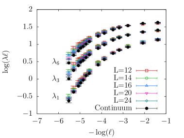
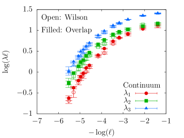
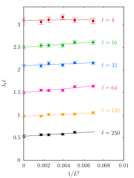
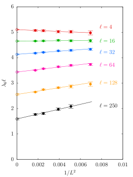
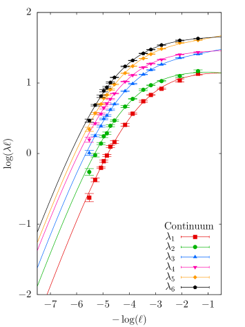
We show the approach to the continuum limit for the improved first and sixth positive eigenvalues, and , at different fixed in Figure 1. We find that the leading lattice corrections are removed by the factor . Using extrapolations, we obtain the continuum limit of the eigenvalues. On the top panel of Figure 2, we show the continuum limit so obtained as a function of , along with the eigenvalues at finite . On the bottom panel of Figure 2, we compare the continuum limits obtained using overlap fermions with our earlier result using massless Wilson Dirac operator Karthik and Narayanan (2016). A good agreement between the two lattice regularizations is seen.
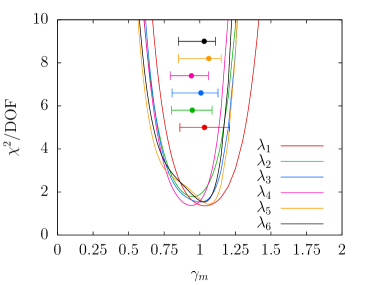
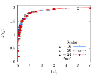
We do not find a simple power-law scaling in the region of where we simulated. We only know the asymptotic dependence of on ; we expect the eigenvalues to behave proportional to for small since the theory is asymptotically free, and as for large . In order to fit the data over the entire range of , we found it convenient to parametrize the dependence on in terms of . Since we do not know the functional dependence of on at any intermediary , we approximate this functional dependence through a rational Padé approximant:
| (35) |
where the ’s are fit parameters. The as a function of is shown in Figure 3. All six low lying eigenvalues predict a value of with confidence. The fit to the data using is shown in Figure 4.
V Inverse Participation Ratio and number variance
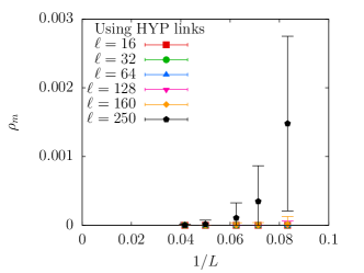
In the absence of a bilinear condensate, there is no ergodic regime in the eigenvalue spectrum of the massless overlap Dirac operator similar to the observations made about the massless Wilson Dirac operator in Karthik and Narayanan (2016). The ergodic regime is characterized by eigenvectors that are completely delocalized and characterized by an IPR defined in Eq. (3) which scales as . A complete localization of the eigenvectors will correspond to a value equal to . Instead, we observe a power law behavior with that is consistent with critical behavior Osborn and Verbaarschot (1998); Al’tschuler and Shklovskii (1986); Al’tschuler et al. (1988); Chalker and Lerner (1996),
| (36) |
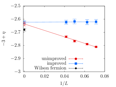
with in the continuum limit as shown in Figure 5. The top panel of Figure 5 shows the finite size scaling of for the eigenvector corresponding to the smallest eigenvalue, as determined on lattice. We find IPR to be one of the few observables which show a simple power-law behavior over a range of we simulated. In the bottom panel, we show the exponent as a function of . The red solid circles are the ones without any improvement, and it shows a leading lattice correction. The continuum extrapolated value corresponds to the one we quoted: . We empirically find the to be removed by using an improved definition, . These are shown by the blue solid square points, which extrapolates to the same value of . The black solid diamond data point corresponds to the value as determined using Wilson-Dirac fermions Karthik and Narayanan (2016). In Figure 6, we show the exponent for the -th eigenvector, for different . We find the finite-size scaling of IPR to be robust across eigenvectors. The small disagreement in between the overlap and Wilson fermion, is not significant compared to the scatter seen in Figure 6.
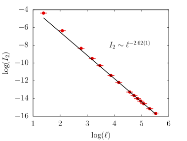
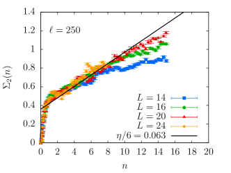
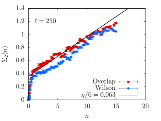
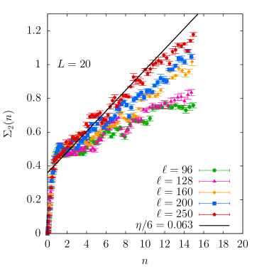
If the low-lying eigenvalues are in the critical regime, then we expect the number variance, , to behave linearly with , with a slope given by . On the left panel of Figure 7, we show the number variance as a function of at at different . We do see some finite lattice spacing effects at larger . The slope of from the finer lattice matches the critical behavior for a wide range of . On the right panel of Figure 7, we compare the result from overlap fermion with the one from the Wilson-Dirac fermion Karthik and Narayanan (2016). The linear behavior is seen for a wider range with overlap fermions. Perhaps, this is because overlap fermions are exactly massless thereby capturing the fluctuations of the low-lying eigenvalues better than the Wilson-Dirac fermions. Finally, we show the -dependence of the number variance in Figure 8 where we see that the slope of the linear rise increases with and approaches the slope . As we noted in Karthik and Narayanan (2016), this trend is opposite to the one expected when a condensate is present.
VI Scalar and vector correlators
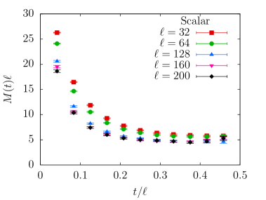
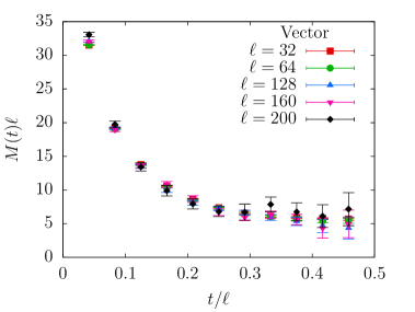
In this section, we study the behavior of the scalar and vector correlators with the aim of lending further support to the scale-invariant nature of the theory. As a start, we attempt to extract a mass using the standard lattice technique Gattringer and Lang (2009) of finding the effective mass, , from the zero-spatial momentum correlators . For a correlator in a periodic lattice, one defines the effective mass using
| (37) |
If the solution, , to the above equation becomes essentially independent of for , then this -independent value, , can be used as an upper bound to the lowest state that contributes to the correlator, . The results for the scalar and vector effective masses are shown in Figure 9. One should note that we have plotted the effective mass times the box size, , on the -axis. There is reasonable evidence for approaching a limit for large . A striking observation is that is essentially independent of the box size . This indicates that the upper bound on the mass in physical units approaches zero in the infinite volume limit for both the scalar and vector correlators 222A fit to both the scalar and vector correlators with two massive states resulted in both of the masses approaching zero in the infinite volume.. Therefore, there is no mass gap in these two sectors of the theory. One could take the point of view that the value of in the plateau of the effective mass plot is actually a mass gap at finite . In such a case, behavior could be explained as the standard hyper-scaling relation for a scale-invariant theory. As for a larger conformal invariance is concerned, such a mass gap could arise by the explicit breaking of conformal symmetry by the finite box size, as shown in two-dimensions Francesco et al. (1999).
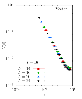
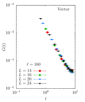
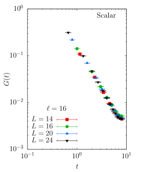
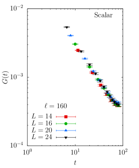
Next, we look at the correlators themselves to see evidence for a power-law behavior. First, we show that the lattice spacing effects in the scalar and vector correlators are under control in Figure 10; the top panels show the vector correlator at different on two box sizes representative of small and large . Similar plots for the scalar are shown in the bottom panels.
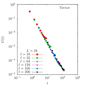
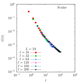
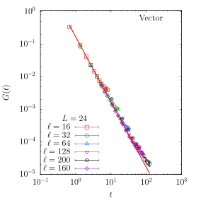
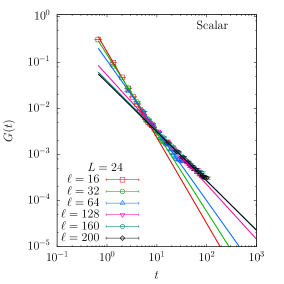
The brute force way to obtain the correlators at infinite volume is to take the limit of the correlators at each , and then take at each physical . Such a procedure is not numerically feasible. Since the lattice artifacts in the correlators are under control, we can use the correlators determined at different on the same lattice to scan a wide range of physical . This is possible provided the dependence of the correlators at fixed are small. Such a reconstruction of infinite volume correlators for the scalar and vector over a range of covering three orders of magnitude are shown in Figure 11. We do see a clear approach to the infinite volume limit at a fixed , after the fact. The vector correlator shows a clean power law behavior, while the scalar does not. However, the scalar correlator in the log-log plot in Figure 11 is concave up, which again rules out the presence of a mass gap because an exponential on a log-log plot is concave down. Thus, we are left with the possibility that the leading scaling behavior for the scalar would set in at even larger values of physical .
Before we further explore the possible power-law behavior at larger separations , we digress to consider the expected behavior of the zero spatial momentum correlator of a primary operator in a conformal field theory. Consider the power-law correlation function,
| (38) |
corresponding to a primary operator of conformal dimension in a CFT. Its zero momentum correlation function will behave as
| (39) |
Both the scalar and vector bilinears have an engineering mass dimension equal to . Since the vector bilinear is associated with a conserved current, it will not acquire any anomalous dimension. Therefore, , and we should find
| (40) |
Since mass acquires an anomalous dimension , the scalar bilinear will also acquire an anomalous dimension such that the sum of the dimensions is equal to . Therefore
| (41) |
We have shown in the previous section that , which along with Eq. (39) and Eq. (41), suggests that
| (42) |
Since the correlator has to vanish as , we see that is marginal for power law behavior which also follows from unitarity constraints in CFTs Mack (1977).
The vector correlator is shown on the left panel of Figure 12. It exhibits a clear power-law behavior over the entire range of the plot — (shown as a red solid line in Figure 12) describes the data well. Thus the vector indeed does not get an anomalous dimension. This might be non-trivial in light of Ref Collins et al. (2006) which was used recently in Janssen (2016) to argue for a possible phase with spontaneously broken Lorentz symmetry.
The scalar correlator is shown on the the right panel of Figure 12. It does not show a simple power law behavior over the entire range. In particular, the behavior at small is quite different from the behavior at large . In order to estimate the asymptotic behavior, we use the following strategy. We numerically estimate the tangent, , on the log-log plot at various values of . We have already shown that the data can be assumed to be the continuum result to a good accuracy. In any region of in Figure 12, data from multiple overlap. Given a fixed value of , we have a set of values that appear on the plot. We use and fit a straight line to the data at a fixed and call that as the tangent, . These are the various colored lines in Figure 12 that correspond to tangents determined using the correlator data from , represented by the same color.
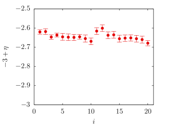
In Figure 13, we show this slope as a function of . We confirm our earlier statement that the data describes the continuum quite well by showing that the results from three different lattice spacings lie on the same curve. The short-distance behavior of the correlator is governed by an exponent . As is increased, the exponent decreases. One could interpret this as a flow from the trivial UV fixed point into a non-trivial infra-red fixed point as the length-scale is increased. Equivalently, the bilinear scalar operator is not a simple primary operator in a conformal field theory but one primary operator dominates the long distance behavior. Using a Padé approximant in , we extrapolate to its infra-red value. We estimate . This corresponds to an estimate of the anomalous dimension of mass from the scalar correlator, . This is in good agreement with the one obtained in Section IV. Our estimate of the mass anomalous dimension from the correlator excludes since the correlator approaches zero as .
VII Conclusions
We have performed a numerical investigation of three dimensional QED coupled to two flavors of two-component massless fermions while preserving parity. We used overlap fermion which preserves the full U symmetry away from the continuum limit. We extracted physical quantities on a three-dimensional continuum torus of size by studying the continuum limit at a fixed . By studying the finite-size scaling of the low-lying eigenvalues of the massless anti-Hermitian overlap Dirac operator, we confirmed the absence of a bilinear condensate that was previously established using Wilson-Dirac fermions Karthik and Narayanan (2016). This enabled us to obtain a value for the mass anomalous dimension, namely, , which is at the upper edge of the allowed value for a conformal field theory. The eigenvectors associated with the low lying eigenvalues of the anti-Hermitian overlap Dirac operator showed critical behavior in the sense of a metal-insulator transition. The scaling behavior of the inverse participation ratio (IPR) of the associated eigenvectors and the linear behavior of number variance of the low lying eigenvalues were consistent with critical behavior. Our analysis of the scalar and vector correlators showed that there is no mass gap in these sectors of the theory. The power law behavior of the vector correlator was consistent with the vector current being conserved. The asymptotic power law behavior of the scalar correlator resulted in an independent estimate of the mass anomalous dimension, namely, .
The analysis performed in this paper along with the results in Karthik and Narayanan (2016) suggests that three dimensional QED with number of two component massless fermions is scale invariant for when ones uses a regularization that preserves parity. In order to consider theories where one has a phase where scale invariance is broken, we plan to extend our studies to non-abelian gauge theories in three dimensions. As a start, we are currently studying three-dimensional SU gauge theories in the large limit where fermions are quenched, provided parity is preserved. Preliminary numerical studies Karthik and Narayanan (in preparation) suggest that there is a non-zero bilinear condensate in this limit. The natural direction we plan to pursue is to map out the phase transition in the - plane that separates a scale invariant phase from one where there is a bilinear condensate. Another direction we plan to pursue is to consider U gauge fields in four dimensions coupled to fermions in three dimensions. The extent of the fourth direction changes the gauge action from the limit considered in this paper where the extent of the fourth direction was set to zero. This is in the spirit of what one is interested in condensed matter physics and it is possible that scale invariance is broken if the fourth direction is large enough. We also plan to perform numerical studies in this direction.
Acknowledgements.
All computations in this paper were made on the JLAB computing clusters under a class B project. The authors acknowledge partial support by the NSF under grant number PHY-1205396 and PHY-1515446. We thank Dam Son and Igor Klebanov for useful discussions.Appendix A Generating functional
We develop the basic formula for the generating function following Narayanan and Neuberger (1995). Although the technical details are not new, the final result shows the explicit form of the propagator for a two-component fermion. Let
| (43) |
We define new sets of creation operators as
| (44) |
and new sets of annihilation operators as
| (45) |
It follows from Eq. (16) and Eq. (17) that
| (46) |
Inverting Eq. (44) and Eq. (45), we arrive at
| (47) |
and
| (48) |
Using the above equations, we can write
| (49) |
where
| (50) |
This split is equivalent to
| (51) |
From the canonical anti-commutation relations, it follows that
| (52) |
Therefore, we have
| (53) | |||||
| (54) | |||||
| (55) | |||||
| (56) |
This result will be used in Appendix B.
Appendix B Introduction of parity invariant mass terms
The partition function for the parity-invariant theory with massless fermions is
| (57) |
Parity invariance is ensured by and . The generating functional for theory with parity invariant mass terms is
| (58) | |||
| (59) | |||
| (60) |
Using standard manipulations of converting the mass terms bilinear in creation-annihilation operators by introducing auxiliary Grassmann fields, and then using the result from Appendix A, the final result is
| (62) | |||||
We proceed to go to a flavor diagonal basis by diagonalizing the mass matrix using
| (63) |
where
| (64) |
The matrix, , is invertible as long as and . Defining flavor diagonal sources as
| (65) |
and noting that
| (66) |
we arrive at Eq. (21).
Appendix C Simulation details
| 4 | 0.032(12) | 0.02233(90) | 0.0182(62) | 0.0091(48) | 0.0067(30) |
|---|---|---|---|---|---|
| 8 | 0.029(10) | 0.0178(87) | 0.0145(72) | 0.0085(41) | 0.0041(31) |
| 16 | 0.028(11) | 0.0186(67) | 0.0133(49) | 0.0055(32) | 0.0022(21) |
| 24 | 0.0326(84) | 0.0185(60) | 0.0137(46) | 0.0068(23) | 0.0033(21) |
| 32 | 0.0435(81) | 0.0299(71) | 0.0222(40) | 0.0126(19) | 0.0053(20) |
| 48 | 0.072(18) | 0.0542(62) | 0.0396(48) | 0.0244(36) | 0.0145(16) |
| 64 | 0.104(10) | 0.0750(85) | 0.0635(45) | 0.0401(37) | 0.0267(21) |
| 96 | 0.164(15) | 0.133(12) | 0.1123(75) | 0.0790(52) | 0.0574(38) |
| 112 | 0.204(17) | 0.165(15) | 0.1337(85) | 0.0996(62) | 0.0747(37) |
| 128 | 0.229(22) | 0.193(16) | 0.1633(86) | 0.1181(53) | 0.0917(47) |
| 144 | 0.255(12) | 0.221(17) | 0.183(12) | 0.1396(91) | 0.1084(52) |
| 160 | 0.268(21) | 0.242(19) | 0.207(14) | 0.1605(78) | 0.1264(65) |
| 200 | 0.323(25) | 0.308(28) | 0.254(14) | 0.206(13) | 0.1659(66) |
| 250 | 0.453(30) | 0.334(23) | 0.297(17) | 0.270(16) | 0.214(12) |
We generated gauge-field configurations using two flavors of dynamical massless overlap fermions in three-dimensional torus with different physical extents using lattices. The parameters and enter the lattice coupling of the non-compact gauge action:
| (67) |
where ’s are related to the physical gauge-fields as . We tabulate the set of and used in this study in Table 1. We used the Sheikhoslami-Wohlert-Wilson-Dirac operator Sheikholeslami and Wohlert (1985), adapted to three-dimensions in Karthik and Narayanan (2016), as the kernel for the overlap Dirac operator.
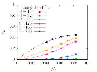
As explained in Karthik and Narayanan (2016), we improved the Sheikhoslami-Wohlert-Wilson-Dirac operator by using one-level HYP smeared ’s in the fermion action Hasenfratz and Knechtli (2001); Hasenfratz et al. (2007). We used the optimal smearing parameters and . Smearing is essential in our study to explore a range of without the exorbitant computational cost of using very large . One can see this by considering the monopole density at finite value of . In a non-compact U theory, monopoles are not physical since they are infinite energy objects, hence they are lattice artifacts. We determined for unsmeared as well as optimal HYP smeared gauge-fields using the procedure outlined in DeGrand and Toussaint (1980). On the left panel of Figure 14, we show that the monopole density in the unsmeared gauge-field indeed increases with at any finite . At the same time, we also check that the monopole density vanishes in the continuum limit at all . One could have avoided using smearing, but lattice artifacts would have been large in the values of we simulated. On the right panel, we show a similar plot for optimal HYP smeared gauge fields. Now, we find that even with one-level of smearing, monopoles are completely removed at all . Since the fermions see only the smeared gauge-fields, it explains why the fermionic observables exhibit small lattice spacing effects. In addition to removing monopole-like defects, smearing also results in a well-defined value of where the smallest eigenvalue of the Sheikhoslami-Wohlert-Wilson-Dirac operator is minimum. We tabulate the values of , which we use to find the normalization factor (refer Eq. (30)), in Table 1.
We tuned the step-size for the leap-frog evolution at run-time such that acceptance was at least 80%. As for the statistics, we generated to trajectories at each simulation point. Then we used only configurations separated by an auto-correlation time, as determined from the smallest eigenvalue . This amounted to 500 to 1000 independent configurations at all the simulation points.
Appendix D HMC force calculation
In this section, we derive the expression for the fermionic HMC force for the case of massless overlap fermions. The fermion force from the pseudo-fermion action in Eq. (29) is
| (68) |
where the link variable is as defined in Karthik and Narayanan (2016) using the non-compact gauge field. The fermion force when a smeared gauge-link is used in the fermion action, as done in this paper, is obtained by the standard chain-rule, as explicitly worked out in Karthik and Narayanan (2016).
Let us define
| (69) |
Then
| (70) |
We use Eq. (27) and to write Eq. (70) as
| (71) |
can be computed approximately using
| (72) |
We use in our computations. Defining
| (73) |
the fermion force becomes
| (74) |
where
| (75) |
As explained in Appendix C, we used Sheikhoslami-Wohlert-Wilson-Dirac operator in place of the unimproved Wilson Dirac operator, .
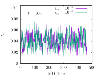
As is well known, there are two kinds of inversions that enter the dynamical overlap simulation — the ones that require the multiple shifted inversion of which we refer to as “inner CG”, and the inversion of which we call the “outer CG”, and it again involves a nested inner CG. We use a stopping criterion that the ratio of the norm of the residue to the norm of the solution vector to be less than . For the inversions required along the molecular dynamics trajectory, we used a stopping criterion for the inner CG, and a stopping criterion for the outer CG. We used a more stringent stopping criterion of and for the inversions required in the computation of fermion action used in the accept-reject step. In Figure 15, we compare the run-time histories of the smallest eigenvalue of the overlap operator at on lattice. Using a starting thermalized configuration, one of the runs was made using and another with . We find that it is sufficient to use the less stringent stopping criterion.
References
- Deser et al. (1982a) S. Deser, R. Jackiw, and S. Templeton, Annals Phys. 140, 372 (1982a).
- Deser et al. (1982b) S. Deser, R. Jackiw, and S. Templeton, Phys.Rev.Lett. 48, 975 (1982b).
- Redlich (1984) A. Redlich, Phys.Rev. D29, 2366 (1984).
- Niemi and Semenoff (1983) A. Niemi and G. Semenoff, Phys.Rev.Lett. 51, 2077 (1983).
- Semenoff (1984) G. W. Semenoff, Phys. Rev. Lett. 53, 2449 (1984).
- Seiberg et al. (2016) N. Seiberg, T. Senthil, C. Wang, and E. Witten (2016), eprint 1606.01989.
- Karch and Tong (2016) A. Karch and D. Tong (2016), eprint 1606.01893.
- Miransky and Shovkovy (2015) V. A. Miransky and I. A. Shovkovy, Phys. Rept. 576, 1 (2015), eprint 1503.00732.
- Castro Neto et al. (2009) A. H. Castro Neto, F. Guinea, N. M. R. Peres, K. S. Novoselov, and A. K. Geim, Rev. Mod. Phys. 81, 109 (2009).
- Franz et al. (2002) M. Franz, Z. Tesanovic, and O. Vafek, Phys. Rev. B66, 054535 (2002), eprint cond-mat/0203333.
- Herbut (2002) I. F. Herbut, Phys. Rev. B66, 094504 (2002), eprint cond-mat/0202491.
- Pisarski (1984) R. D. Pisarski, Phys.Rev. D29, 2423 (1984).
- Appelquist et al. (1985) T. Appelquist, M. J. Bowick, E. Cohler, and L. C. R. Wijewardhana, Phys. Rev. Lett. 55, 1715 (1985).
- Appelquist et al. (1986a) T. W. Appelquist, M. J. Bowick, D. Karabali, and L. C. R. Wijewardhana, Phys. Rev. D33, 3704 (1986a).
- Appelquist et al. (1986b) T. Appelquist, M. J. Bowick, D. Karabali, and L. C. R. Wijewardhana, Phys. Rev. D33, 3774 (1986b).
- Appelquist et al. (1988) T. Appelquist, D. Nash, and L. C. R. Wijewardhana, Phys. Rev. Lett. 60, 2575 (1988).
- Kotikov et al. (2016) A. V. Kotikov, V. I. Shilin, and S. Teber (2016), eprint 1605.01911.
- Braun et al. (2014) J. Braun, H. Gies, L. Janssen, and D. Roscher, Phys.Rev. D90, 036002 (2014), eprint 1404.1362.
- Appelquist et al. (1999) T. Appelquist, A. G. Cohen, and M. Schmaltz, Phys. Rev. D60, 045003 (1999), eprint hep-th/9901109.
- Appelquist and Wijewardhana (2004) T. Appelquist and L. C. R. Wijewardhana, in Proceedings, 3rd International Symposium on Quantum theory and symmetries (QTS3) (2004), pp. 177–191, eprint hep-ph/0403250.
- Giombi et al. (2015) S. Giombi, I. R. Klebanov, and G. Tarnopolsky (2015), eprint 1508.06354.
- Giombi et al. (2016) S. Giombi, G. Tarnopolsky, and I. R. Klebanov (2016), eprint 1602.01076.
- Di Pietro et al. (2016) L. Di Pietro, Z. Komargodski, I. Shamir, and E. Stamou, Phys. Rev. Lett. 116, 131601 (2016), eprint 1508.06278.
- Herbut (2016) I. F. Herbut (2016), eprint 1605.09482.
- Chester and Pufu (2016) S. M. Chester and S. S. Pufu (2016), eprint 1603.05582.
- Hands et al. (2002) S. Hands, J. Kogut, and C. Strouthos, Nucl.Phys. B645, 321 (2002), eprint hep-lat/0208030.
- Hands et al. (2004) S. Hands, J. Kogut, L. Scorzato, and C. Strouthos, Phys.Rev. B70, 104501 (2004), eprint hep-lat/0404013.
- Raviv et al. (2014) O. Raviv, Y. Shamir, and B. Svetitsky, Phys. Rev. D90, 014512 (2014), eprint 1405.6916.
- Karthik and Narayanan (2016) N. Karthik and R. Narayanan, Phys. Rev. D93, 045020 (2016), eprint 1512.02993.
- Hands (2016) S. Hands, Phys. Lett. B754, 264 (2016), eprint 1512.05885.
- Hands (2015) S. Hands, JHEP 09, 047 (2015), eprint 1507.07717.
- Narayanan and Nishimura (1997) R. Narayanan and J. Nishimura, Nucl.Phys. B508, 371 (1997), eprint hep-th/9703109.
- Kikukawa and Neuberger (1998) Y. Kikukawa and H. Neuberger, Nucl.Phys. B513, 735 (1998), eprint hep-lat/9707016.
- Mack (1977) G. Mack, Commun. Math. Phys. 55, 1 (1977).
- Osborn and Verbaarschot (1998) J. C. Osborn and J. J. M. Verbaarschot, Nucl. Phys. B525, 738 (1998), eprint hep-ph/9803419.
- Al’tschuler and Shklovskii (1986) B. Al’tschuler and B. Shklovskii, Sov. Phys. JETP 64, 127 (1986).
- Al’tschuler et al. (1988) B. Al’tschuler, I. Zharekeshev, S. Kotochigova, and B. Shklovskii, Sov. Phys. JETP 67, 625 (1988).
- Chalker and Lerner (1996) V. Chalker, J.T. amd Kravtsov and I. Lerner, Pis’ma v ZhETF 64, 355 (1996).
- Narayanan and Neuberger (1995) R. Narayanan and H. Neuberger, Nucl.Phys. B443, 305 (1995), eprint hep-th/9411108.
- Karthik and Narayanan (2015) N. Karthik and R. Narayanan, Phys. Rev. D92, 025003 (2015), eprint 1505.01051.
- Kalkreuter and Simma (1996) T. Kalkreuter and H. Simma, Comput. Phys. Commun. 93, 33 (1996), eprint hep-lat/9507023.
- van den Eshof et al. (2002) J. van den Eshof, A. Frommer, T. Lippert, K. Schilling, and H. A. van der Vorst, Comput. Phys. Commun. 146, 203 (2002), eprint hep-lat/0202025.
- Chiu et al. (2002) T.-W. Chiu, T.-H. Hsieh, C.-H. Huang, and T.-R. Huang, Phys. Rev. D66, 114502 (2002), eprint hep-lat/0206007.
- Edwards et al. (1999) R. G. Edwards, U. M. Heller, and R. Narayanan, Phys.Rev. D59, 094510 (1999), eprint hep-lat/9811030.
- Gattringer and Lang (2009) C. Gattringer and C. Lang, Quantum chromodynamics on the lattice: An introductory presentation (lecture notes in physics vol. 788) (2009).
- Francesco et al. (1999) P. Francesco, P. Mathieu, and D. Senechal, Conformal field theory, graduate texts in contemporary physics (1999).
- Collins et al. (2006) J. C. Collins, A. V. Manohar, and M. B. Wise, Phys. Rev. D73, 105019 (2006), eprint hep-th/0512187.
- Janssen (2016) L. Janssen (2016), eprint 1604.06354.
- Karthik and Narayanan (in preparation) N. Karthik and R. Narayanan (in preparation).
- Sheikholeslami and Wohlert (1985) B. Sheikholeslami and R. Wohlert, Nucl. Phys. B259, 572 (1985).
- Hasenfratz and Knechtli (2001) A. Hasenfratz and F. Knechtli, Phys. Rev. D64, 034504 (2001), eprint hep-lat/0103029.
- Hasenfratz et al. (2007) A. Hasenfratz, R. Hoffmann, and S. Schaefer, JHEP 05, 029 (2007), eprint hep-lat/0702028.
- DeGrand and Toussaint (1980) T. A. DeGrand and D. Toussaint, Phys. Rev. D22, 2478 (1980).