The Higgs transverse momentum spectrum with finite quark masses beyond leading order

Abstract

We apply the leading-log high-energy resummation technique recently derived by some of us to the transverse momentum distribution for production of a Higgs boson in gluon fusion. We use our results to obtain information on mass-dependent corrections to this observable, which is only known at leading order when exact mass dependence is included. In the low $p_{\rm\scriptscriptstyle\rm T}$ region we discuss the all-order exponentiation of collinear bottom mass logarithms. In the high $p_{\rm\scriptscriptstyle\rm T}$ region we show that the infinite top mass approximation loses accuracy as a power of $p_{\rm\scriptscriptstyle\rm T}$, while the accuracy of the high-energy approximation is approximately constant as $p_{\rm\scriptscriptstyle\rm T}$ grows. We argue that a good approximation to the NLO result for $p_{T}\gtrsim 200$ GeV can be obtained by combining the full LO result with a $K$-factor computed using the high-energy approximation.

1 Introduction

The discovery of the Higgs boson at the CERN Large Hadron Collider (LHC) Aad:2012tfa ; Chatrchyan:2012xdj set an important milestone for our understanding of fundamental interactions. So far, the properties of the new particle seem consistent with Standard Model predictions, which suggests a simple electroweak symmetry breaking sector Aad:2015gba ; Khachatryan:2014jba . A major goal of the LHC Run II is establish whether the new particle is indeed the Higgs Boson of the Standard Model or there are some deviations pointing towards new physics. In order to reach this goal, very precise theoretical predictions for signal and background processes are mandatory.

The dependence of the cross-section on heavy quark masses is an interesting probe of the properties of the Higgs boson both within and beyond the Standard Model, since it gives access to the structure of the $ggH$ coupling Arnesen:2008fb ; Dolan:2012rv ; Grojean:2013nya ; Englert:2013vua ; Harlander:2013oja ; Wiesemann:2015fxy . A particularly interesting observable in this respect is the transverse momentum distribution, since it allows a study of the $ggH$ coupling at different energy scales and can then provide valuable information on its structure.

Gluon fusion is the main Higgs production mechanism at the LHC. In this channel the total production cross-section was recently computed to N³LO accuracy Anastasiou:2015ema ; Anastasiou:2016cez . Recently, fully differential results for Higgs production in association with one hard jet have become available Boughezal:2015dra ; Boughezal:2015aha ; Chen:2014gva . However, all these results have been obtained in the approximation in which heavy quark masses are assumed to be very large, and the coupling of the Higgs boson to gluons is then described using an effective theory.

At the inclusive level, this is just as well since the dependence on the heavy quark mass is very weak and under good theoretical control at present collider energies Harlander:2009my . On the other hand, large effects are expected in the transverse momentum distribution. Indeed, theoretical predictions for this observable in the full theory, which are only known at the lowest nontrivial order Baur:1989cm , show large deviations from the effective theory as soon as $p_{\rm\scriptscriptstyle\rm T}$ is comparable to the top quark mass. The fact that only the leading order is known is particularly problematic since we know from the inclusive case that radiative corrections are very large.

In Ref. Marzani:2008az some of us have shown that using high-energy resummation methods it is possible to glean partial information on the heavy quark mass dependence at higher order, at the level of the inclusive cross-section. These results were subsequently used to construct an optimized approximation to the NNLO Harlander:2009mq ; Harlander:2009my ; Pak:2009dg and N³LO Ball:2013bra ; Bonvini:2014jma ; Bonvini:2016frm ; Harlander:2016hcx inclusive cross-section with full top mass dependence. The goal of this paper is to apply similar ideas to transverse momentum distributions; this is possible thanks to the recent derivation Forte:2015gve of high-energy resummation for transverse momentum distributions.

High-energy resummation is available only at the leading logarithmic level: it provides us with information on the contribution to all orders in $\alpha_{s}$ which carries the highest logarithmic power of $\ln\frac{s}{m_{h}^{2}}$. Still, this provides relevant insight on the heavy quark mass dependence. Indeed, in the opposite kinematic limit, namely the threshold limit in which $\frac{m_{h}^{2}}{s}\to 1$, all the dependence on the heavy quark mass can be absorbed in a factorized Wilson coefficient which depends only on the strong coupling and the ratio of the heavy quark to the Higgs mass, up to terms suppressed by powers of $1-\frac{m_{h}^{2}}{s}$. On the contrary, in the high-energy limit the behaviour of the total cross-section in the effective and full theory are qualitatively different, as the former is double-logarithmic Hautmann:2002tu and the latter single-logarithm Marzani:2008az (i.e. they are respectively a series in $\alpha_{s}\ln^{2}\frac{s}{m_{h}^{2}}$ and $\alpha_{s}\ln\frac{s}{m_{h}^{2}}$).

In Ref. Forte:2015gve , where a general resummation of transverse momentum distributions was derived, a first application to Higgs production in gluon fusion in the effective field theory limit was presented. Here, we will apply the same general formalism to the same observable, but now retaining full heavy quark mass dependence. Besides studying the top mass dependence in the boosted Higgs region, our results provide some insight on bottom logs when both top and bottom mass dependence is retained. Indeed, in the region $m_{b}^{2}\lesssim p_{\rm\scriptscriptstyle\rm T}^{2}$ bottom mass effects may become relevant. Of particular interest is the region $m_{b}^{2}<p_{\rm\scriptscriptstyle\rm T}^{2}<m_{h}^{2}$, in which logarithmically enhanced, though mass-suppressed terms appear Banfi:2013eda . We will be able to study these logs to all orders, albeit in the high-energy limit.

The paper is organized as follow: in Sect. 2 we present the resummation of the transverse momentum distribution for Higgs production in gluon fusion with complete quark mass dependence. In Sect. 3 we discuss the partonic resummed cross-section. We check that its leading order truncation agrees with the high-energy limit of the exact result, and that in the pointlike limit it reproduces the resummed result of Ref. Forte:2015gve . We study the first few orders of its perturbative expansion, and specifically we study the high-$p_{\rm\scriptscriptstyle\rm T}$ region and compare the high-energy result expanded through NLO in the effective and full theory. We use these result as a way to qualitatively estimate mass corrections beyond leading order: we show that for high enough transverse momenta the high-energy approximation provides a reasonable estimate of higher-order corrections while the effective field theory fails completely. We also address to all orders the structure of the logarithmic dependence on the bottom mass. In Sect. 4 we discuss phenomenological implications: we repeat the comparison of various approximations of Sect. 3 but now at the level of hadronic cross-sections and $K$-factors. We conclude that currently the best approximation in the high $p_{T}\gtrsim 200$ GeV region is obtained by combining the exact LO result with a $K$-factor determined in the high-energy approximation. We also compare our results to previous estimates of finite mass effects based on matching to parton showers Hamilton:2015nsa . More accurate approximations could be obtained by combining multiple resummations, as we discuss in Sect. 5 where conclusions are drawn and future developments are discussed.

2 Resummation

Leading-log high-energy resummation has been known for inclusive cross-sections Catani:1990xk ; Catani:1990eg and rapidity distributions Caola:2010kv since a long time. More recently, a framework for the resummation of transverse-momentum spectra was developed by some of us Forte:2015gve . In this section, after a brief summary of notation and conventions, we apply it to the resummation of the Higgs transverse momentum distribution in gluon fusion with finite top and bottom masses, and then study its perturbative expansion, which will allow us to obtain the truncation of the resummed result to any finite order.

2.1 Kinematics and definitions

In standard collinear factorization, the hadron-level transverse momentum distribution can be written as

$$\frac{d\sigma}{d\xi_{p}}\left(\tau,\xi_{p},\{y_{i}\}\right)=\sum_{ij}\int_{\tau\left(\sqrt{1+\xi_{p}}+\sqrt{\xi_{p}}\right)^{2}}^{1}dx_{1}\int_{\frac{\tau\left(\sqrt{1+\xi_{p}}+\sqrt{\xi_{p}}\right)^{2}}{x_{1}}}^{1}dx_{2}\\ \times\frac{d\bar{\sigma}_{ij}}{d\xi_{p}}\left(\frac{\tau}{x_{1}x_{2}},\xi_{p},\{y_{i}\},\alpha_{s}(\mu_{\rm\scriptscriptstyle\rm R}^{2}),\mu_{\rm\scriptscriptstyle\rm R}^{2},\mu_{\rm\scriptscriptstyle\rm F}^{2}\right)f_{i}\left(x_{1},\mu_{\rm\scriptscriptstyle\rm F}^{2}\right)f_{j}\left(x_{2},\mu_{\rm\scriptscriptstyle\rm F}^{2}\right),$$ (2.1)

where $f_{i}(x_{i})$ are parton distributions and we parametrized the kinematics in terms of the following dimensionless ratios

$$\tau=\frac{m_{h}^{2}}{s};\>\xi_{p}=\frac{p_{\rm\scriptscriptstyle\rm T}^{2}}{m_{h}^{2}};\>y_{i}=\frac{m_{i}^{2}}{m_{h}^{2}}$$ (2.2)

where $m_{h}$, $m_{i}$ are respectively the Higgs and the various heavy quark masses, $p_{\rm\scriptscriptstyle\rm T}$ is the transverse momentum of the outgoing Higgs boson and $s$ is the (hadronic) center-of-mass energy.

Equation (2.1) can be cast in the form of a standard convolution by an appropriate choice of hard scale. To see this, we define

$$\tau^{\prime}(\tau,\xi_{p})=\tau\left(\sqrt{1+\xi_{p}}+\sqrt{\xi_{p}}\right)^{2}=\frac{Q^{2}}{s},$$ (2.3)

thus identifying the threshold energy

$$\sqrt{Q^{2}}=\sqrt{m_{H}^{2}+p_{\rm\scriptscriptstyle\rm T}^{2}}+\sqrt{p_{\rm\scriptscriptstyle\rm T}^{2}}$$ (2.4)

with the physical scale of the process. Note that when $p_{\rm\scriptscriptstyle\rm T}\ll m_{H}$, $\tau^{\prime}\approx\tau$, while when $p_{\rm\scriptscriptstyle\rm T}\gg m_{H}$, $\tau^{\prime}\approx\frac{4p_{\rm\scriptscriptstyle\rm T}^{2}}{s}$. If we now introduce the partonic equivalent of Eq. (2.3)

$$x^{\prime}=\frac{Q^{2}}{\hat{s}},$$ (2.5)

we can rewrite the hadronic cross-section as

$$\frac{d\sigma}{d\xi_{p}}\left(\tau,\xi_{p},\{y_{i}\}\right)=\tau^{\prime}\sum_{ij}\int_{\tau^{\prime}}^{1}\frac{dx^{\prime}}{x^{\prime}}\mathcal{L}_{ij}\left(\frac{\tau^{\prime}}{x^{\prime}},\mu_{\rm\scriptscriptstyle\rm F}^{2}\right)\left[\frac{1}{x^{\prime}}\frac{d\hat{\sigma}_{ij}}{d\xi_{p}}\left(x^{\prime},\xi_{p},\{y_{i}\},\alpha_{s}(\mu_{\rm\scriptscriptstyle\rm R}^{2}),\mu_{\rm\scriptscriptstyle\rm R}^{2},\mu_{\rm\scriptscriptstyle\rm F}^{2}\right)\right],$$ (2.6)

where the parton luminosity is defined in the usual way as

$$\mathcal{L}_{ij}\left(x,\mu_{\rm\scriptscriptstyle\rm F}^{2}\right)=\int_{x}^{1}\frac{dy}{y}f_{i}\left(y,\mu_{\rm\scriptscriptstyle\rm F}^{2}\right)f_{j}\left(\frac{x}{y},\mu_{\rm\scriptscriptstyle\rm F}^{2}\right),$$ (2.7)

and

$$\frac{d\hat{\sigma}_{ij}}{d\xi_{p}}\left(x^{\prime},\xi_{p},\{y_{i}\},\alpha_{s},\mu_{\rm\scriptscriptstyle\rm R}^{2},\mu_{\rm\scriptscriptstyle\rm F}^{2}\right)=\frac{d\bar{\sigma}_{ij}}{d\xi_{p}}\left(\frac{x^{\prime}}{\left(\sqrt{1+\xi_{p}}+\sqrt{\xi_{p}}\right)^{2}},\xi_{p},\{y_{i}\},\alpha_{s},\mu_{\rm\scriptscriptstyle\rm R}^{2},\mu_{\rm\scriptscriptstyle\rm F}^{2}\right).$$ (2.8)

That $Q^{2}$ is a natural choice for the process is demonstrated by the fact that Eq. (2.6) takes the form of a convolution, and thus in particular it factorizes upon Mellin transformation. In the following, we fix $\mu_{\rm\scriptscriptstyle\rm R}^{2}=\mu_{\rm\scriptscriptstyle\rm F}^{2}=Q^{2}$ and drop for simplicity the dependencies on these scales. The full scale dependence can be restored at any stage using renormalization group arguments.

High-energy resummation is usually performed in Mellin ($N$) space. For the sake of the determination of the leading-logarithmic (LL$x$) result, it is immaterial whether the scale is chosen as $Q^{2}$ Eq. (2.4) (so the Mellin $N$ variable is conjugate to $\tau^{\prime}$ Eq. (2.3)) or $m_{H}^{2}$ (so Mellin $N$ is conjugate to $\tau$ Eq. (2.2)), because the choice of scale is a subleading $\ln x$ effect. The LL$x$ expression of the partonic cross-section can be expressed in terms of the Mellin transform

$$\frac{d{\hat{\sigma}}_{ij}}{d\xi_{p}}\left(N,\xi_{p},\{y_{i}\},\alpha_{s}\right)=\int_{0}^{1}dx\,x^{N-1}\frac{d\hat{\sigma}_{ij}}{d\xi_{p}}\left(x,\xi_{p},\{y_{i}\},\alpha_{s}\right)$$ (2.9)

through an impact factor $h_{p_{\rm\scriptscriptstyle\rm T}}$:

$$\frac{d\hat{\sigma}_{ij}}{d\xi_{p}}\left(N,\xi_{p},\{y_{i}\},\alpha_{s}\right)=h_{ij,p_{\rm\scriptscriptstyle\rm T}}\left(0,\gamma\left(\frac{\alpha_{s}}{N}\right),\gamma\left(\frac{\alpha_{s}}{N}\right),\xi_{p},\{y_{i}\}\right),$$ (2.10)

where $\gamma\left(\frac{\alpha_{s}}{N}\right)$ is the BFKL LL$x$ resummed anomalous dimension Lipatov:1976zz ; Fadin:1975cb ; Kuraev:1976ge ; Kuraev:1977fs ; Balitsky:1978ic ; Altarelli:1999vw . The impact factor for the $gg$ channel is defined as

$$h_{gg,p_{\rm\scriptscriptstyle\rm T}}\left(N,M_{1},M_{2},\xi_{p},\{y_{i}\}\right)=h_{p_{\rm\scriptscriptstyle\rm T}}\left(N,M_{1},M_{2},\xi_{p},\{y_{i}\}\right)=M_{1}M_{2}R\left(M_{1}\right)R\left(M_{2}\right)\times\\ \times\int_{0}^{\infty}d\xi\,\xi^{M_{1}-1}\int_{0}^{\infty}d\bar{\xi}\,\bar{\xi}^{M_{2}-1}\,C_{p_{\rm\scriptscriptstyle\rm T}}\left(N,\xi,\bar{\xi},\xi_{p},\{y_{i}\}\right).$$ (2.11)

Here the process-dependent coefficient function $C_{p_{\rm\scriptscriptstyle\rm T}}$ describes the interaction of two hard off-shell gluons with the Higgs boson (its computation will be described in the next Subsection), the Mellin transforms in $\xi$ and $\bar{\xi}$ resum multiple high-energy gluon emission and $R(M)$ is a function which fixes the factorization scheme; the reader is referred to Ref. Forte:2015gve for full derivations and details.

Due to the eikonal nature of high-energy gluon evolution, results for all other partonic channels can be trivially obtained from Eq. (2.11):

$$h_{qg,p_{\rm\scriptscriptstyle\rm T}}(N,M_{1},M_{2},\xi_{p},\{y_{i}\})= \frac{C_{F}}{C_{A}}\bigg{[}h_{p_{\rm\scriptscriptstyle\rm T}}(N,M_{1},M_{2},\xi_{p},\{y_{i}\})-h_{p_{\rm\scriptscriptstyle\rm T}}(N,0,M_{2},\xi_{p},\{y_{i}\})\bigg{]},$$ (2.12)

$$h_{qq^{\prime},p_{\rm\scriptscriptstyle\rm T}}(N,M_{1},M_{2},\xi_{p},\{y_{i}\})= \left(\frac{C_{F}}{C_{A}}\right)^{2}\bigg{[}h_{p_{\rm\scriptscriptstyle\rm T}}(N,M_{1},M_{2},\xi_{p},\{y_{i}\})+$$

$$-h_{p_{\rm\scriptscriptstyle\rm T}}(N,0,M_{2},\xi_{p},\{y_{i}\})-h_{p_{\rm\scriptscriptstyle\rm T}}(N,M_{1},0,\xi_{p},\{y_{i}\})],$$ (2.13)

where $q,q^{\prime}$ can be any quark or anti-quark. The subtraction terms in Eq. (2.12) ensure that at least one emission from the quark line is present, see Ref. Forte:2015gve for details; note that subtraction of $h_{p_{\rm\scriptscriptstyle\rm T}}(N,0,0,\xi_{p},\{y_{i}\})$ is not necessary because this contribution vanishes for $p_{\rm\scriptscriptstyle\rm T}\not=0$.

2.2 The impact factor

The computation of the coefficient function $C_{p_{\rm\scriptscriptstyle\rm T}}$ which enters Eq. (2.11) follows the procedure outlined in Refs. Marzani:2008az ; Forte:2015gve : $C_{p_{\rm\scriptscriptstyle\rm T}}$ is closely related to the transverse momentum distribution for the process

$$g^{*}\left(k_{1}\right)+g^{*}\left(k_{2}\right)\to H\left(p\right).$$ (2.14)

Specifically, the off-shell gluon momenta can be parametrized in terms of longitudinal and transverse components as

$$k_{1}=zp_{1}+k_{t,1}$$

$$k_{2}=\bar{z}p_{2}+k_{t,2}$$ (2.15)

with

$$p_{i}^{2}=0,\quad p_{i}\cdot k_{t,j}=0,\quad i,j=1,2$$

$$k_{1}^{2}=k_{t,1}^{2}=-\xi m_{h}^{2}<0,\quad k_{2}^{2}=k_{t,2}^{2}=-\bar{\xi}m_{h}^{2}<0\quad 2p_{1}\cdot p_{2}=\hat{s},$$

$$k_{t,1}\cdot k_{t,2}=-\sqrt{\xi\bar{\xi}}m_{h}^{2}\cos\theta.$$

The coefficient function $C_{p_{\rm\scriptscriptstyle\rm T}}(N,\xi,\bar{\xi},\xi_{p},\{y_{i}\})$ is then defined as the Mellin transform

$$C_{p_{\rm\scriptscriptstyle\rm T}}(N,\xi,\bar{\xi},\xi_{p},\{y_{i}\})=\int_{0}^{1}dxx^{N-1}C_{p_{\rm\scriptscriptstyle\rm T}}(w,\xi,\bar{\xi},\xi_{p},\{y_{i}\})$$ (2.16)

where

$$x=\frac{m_{h}^{2}}{\hat{s}z\bar{z}}.$$ (2.17)

Note that Mellin transformation in Eq. (2.16) is performed for simplicity with respect to the standard $p_{\rm\scriptscriptstyle\rm T}$-independent scaling variable Eq. (2.17) as in the inclusive computation of Ref. Marzani:2008az : as already mentioned, computing the Mellin transform with respect to the variable $x^{\prime}$ Eq. (2.5) would lead to a result which differs by subleading terms, and thus to the same final LL$x$ answer.

The quantity $C_{p_{\rm\scriptscriptstyle\rm T}}(x,\xi,\bar{\xi},\xi_{p},\{y_{i}\})$ in Eq. (2.16) is the transverse momentum distribution

$$C_{p_{\rm\scriptscriptstyle\rm T}}(x,\xi,\bar{\xi},\xi_{p},\{y_{i}\}) =\int\frac{1}{2\hat{s}z\bar{z}}\times\left[\frac{1}{256}\sum_{\rm col,pol}|M(g^{*}g^{*}\to H)|^{2}\right]\times$$

$$\times d\mathcal{P}(k_{1}+k_{2}\to p_{h})\times\delta\left(\xi_{p}-\xi-\bar{\xi}-2\sqrt{\xi\bar{\xi}}\cos\theta\right).$$ (2.18)

In Eq. (2.2) $d\mathcal{P}$ is the phase space factor

$$d\mathcal{P}(k_{1}+k_{2}\to p_{h})=\frac{2\pi}{m_{h}^{2}}\delta\left(\frac{1}{x}-1-\xi-\bar{\xi}-2\sqrt{\xi\bar{\xi}}\cos\theta\right)\frac{d\theta}{2\pi};$$ (2.19)

the sum over off-shell gluon polarizations is performed using

$$\sum_{\rm\lambda}\epsilon^{\mu}_{\lambda}(k_{i})\epsilon^{\nu*}_{\lambda}(k_{i})=-2\frac{k_{t,i}^{\mu}k_{t,i}^{\nu}}{k_{t,i}^{2}};$$ (2.20)

and the flux factor is determined on the surface orthogonal to $p_{1,2}$.

After standard algebraic manipulations, $C_{p_{\rm\scriptscriptstyle\rm T}}$ can be written as

$$C_{p_{\rm\scriptscriptstyle\rm T}}\left(N,\xi,\bar{\xi},\xi_{p},\{y_{i}\}\right)=2\sigma_{0}\left(\{y_{i}\}\right)\int_{0}^{1}dx\,x^{N-2}\int_{0}^{2\pi}\frac{d\theta}{2\pi}\tilde{F}\left(\xi,\bar{\xi},\xi_{p},\{y_{i}\}\right)\\ \delta\left(\frac{1}{x}-1-\xi_{p}\right)\delta\left(\xi_{p}-\xi-\bar{\xi}-2\sqrt{\xi\bar{\xi}}\cos\theta\right),$$ (2.21)

where $\sigma_{0}$ is the LO Higgs production cross-section

$$\sigma_{0}\left(\{y_{i}\}\right)=\sigma_{0}^{\rm PL}\left|\,\sum_{\{y_{i}\}}K\left(y_{i}\right)\,\right|^{2},$$ (2.22)

$$\sigma_{0}^{\rm PL} =\frac{G_{\scriptscriptstyle\rm F}\sqrt{2}\alpha_{s}^{2}}{576\pi};$$ (2.23)

$$K\left(y\right) =6y\left(1-\frac{1}{4}\left(1-4y\right)\ln^{2}\frac{\sqrt{1-4y}-1}{\sqrt{1-4y}+1}\right).$$ (2.24)

In Eq. (2.23) (as well as in all the remaining Equations in this paper) the branch cut in the logarithm should be handled by giving $y$ a small negative imaginary part. The rather lengthy explicit formula for the form factor $\tilde{F}$ is reported in Appendix A, together with some limiting cases. Note that the quark mass dependence is contained both in the Born cross-section $\sigma_{0}$ and in the form factor $\tilde{F}$. Note also that if the exact quark mass dependence is retained, the form factor $\tilde{F}$ vanishes in the $\xi,\bar{\xi}\to\infty$ limit, while it approaches a constant ($\tilde{F}\to\cos^{2}\theta$) in the pointlike approximation. This fact leads to a qualitatively different high-energy behaviour in the two cases, which we will discuss in detail in the next Sections.

Inserting the expression Eq. (2.21) for the coefficient function $C_{p_{\rm\scriptscriptstyle\rm T}}$ in the impact factor Eq. (2.11) and using one delta function to perform the $x$ Mellin integral we obtain

$$h_{p_{\rm\scriptscriptstyle\rm T}}\left(N,M_{1},M_{2},\xi_{p},\{y_{i}\}\right)=\sigma_{0}\left(\{y_{i}\}\right)M_{1}M_{2}R\left(M_{1}\right)R\left(M_{2}\right)\frac{\xi_{p}^{M_{1}+M_{2}-1}}{\left(1+\xi_{p}\right)^{N}}\int_{0}^{\infty}d\xi_{1}\,\xi_{1}^{M_{1}-1}$$

$$\int_{0}^{\infty}d\xi_{2}\,\xi_{2}^{M_{2}-1}\int_{-1}^{1}\frac{du}{\sqrt{1-u^{2}}}\,\frac{2}{\pi}F\left(\xi_{1},\xi_{2},\xi_{p},\{y_{i}\}\right)\delta\left(1-\xi_{1}-\xi_{2}-2\sqrt{\xi_{1}\xi_{2}}\,u\right),$$ (2.25)

where we have introduced

$$u=\cos\theta,\leavevmode\nobreak\ \leavevmode\nobreak\ \leavevmode\nobreak\ \xi_{1}=\frac{\xi}{\xi_{p}}=-\frac{k_{t,1}^{2}}{p_{\rm\scriptscriptstyle\rm T}^{2}},\leavevmode\nobreak\ \leavevmode\nobreak\ \leavevmode\nobreak\ \xi_{2}=\frac{\bar{\xi}}{\xi_{p}}=-\frac{k_{t,2}^{2}}{p_{\rm\scriptscriptstyle\rm T}^{2}}$$ (2.26)

and defined

$$F\left(\xi_{1},\xi_{2},\xi_{p},\{y_{i}\}\right)=\tilde{F}\left(\xi,\bar{\xi},\xi_{p},\{y_{i}\}\right).$$ (2.27)

We have performed several checks on Eq. (2.2). Using the expressions in Appendix A it is easy to see that in the $y_{i}\to\infty$ limit Eq. (2.2) correctly reproduces the pointlike result of Ref. Forte:2015gve . Also, upon integration over $\xi_{p}$ it reproduces the inclusive result of Ref. Marzani:2008az . Finally, it is clear from Eq. (2.26) that the $\xi_{p}\to 0$ limit at fixed $\xi_{1,2}$ can be treated in the eikonal approximation. As explained in Ref. Forte:2015gve , in this limit the result with full heavy quark mass dependence must reduce to that of the effective theory, up to a Wilson loop prefactor, i.e., the impact factor Eq. (2.2) reduces to the pointlike result, up to the replacement of the Born cross-section Eq. (2.22) with its pointlike form. Comparing to the pointlike impact factor, as given in Eqs. (4.3,4.5) of Ref. Forte:2015gve , this implies the consistency condition

$$\lim_{\xi_{p}\to 0}F\left(\xi_{1},\xi_{2},\xi_{p},y_{t}\right)=\left(\frac{1-\xi_{1}-\xi_{2}}{2\sqrt{\xi_{1}\xi_{2}}}\right)^{2}$$ (2.28)

which can be explicitly checked using the formulas in Appendix A.

2.3 Perturbative expansion

The perturbative expansion of the impact factor which leads to the resummed result can now be obtained by performing the integrations in Eq. (2.2). For the sake of extracting the first several orders in the expansion of the cross-section in powers of $\alpha_{s}$ we are interested in, we need the expansion of the impact factor in powers of $M_{i}$. This task is not entirely straightforward because of the $1/M_{i}$ collinear singularities coming from the $\xi_{i}^{M_{i}-1}$ terms. Although the actual singularities are removed by the $M_{i}R(M_{i})$ factorization terms, they prevent a naive Taylor expansion in $M_{i}$. In Ref. Forte:2015gve this problem was circumvented by analytically computing the impact factor for arbitrary values of $M_{i}$. In the present case, however, an analytic computation does not appear viable because of the complexity of $F$ when the full quark mass dependence is retained.

In order to extract the desired coefficients in the expansion of the impact factor we then proceed as follows. First, we note that because of the kinematics in the LL$x$ limit we cannot have collinear singularities in both $\xi_{1}$ and $\xi_{2}$ at the same time. This is because the transverse momentum of the two incoming off-shell gluons must exactly balance the Higgs transverse momentum, so we cannot have $\xi_{1}=\xi_{2}=0$ and $\xi_{p}\neq 0$ at the same time. This is made explicit by the delta constraint in Eq. (2.2). It is then natural to split the integration domain in two regions, one with $\xi_{1}>\xi_{2}$ and another with $\xi_{2}>\xi_{1}$. In the first one, we define $\xi_{2}=z\xi_{1}$ and rewrite Eq. (2.2) as

$$h^{I}_{p_{\rm\scriptscriptstyle\rm T}}\left(N,M_{1},M_{2},\xi_{p},\{y_{i}\}\right)=\sigma_{0}\left(\{y_{i}\}\right)M_{1}M_{2}R\left(M_{1}\right)R\left(M_{2}\right)\frac{\xi_{p}^{M_{1}+M_{2}-1}}{\left(1+\xi_{p}\right)^{N}}\int_{0}^{1}dz\,z^{M_{2}-1}$$

$$\int_{-1}^{1}\frac{2du}{\pi\sqrt{1-u^{2}}}\int_{0}^{\infty}d\xi_{1}\,\xi_{1}^{M_{1}+M_{2}-1}F\left(\xi_{1},z\xi_{1},\xi_{p},\{y_{i}\}\right)\delta\left(1-\xi_{1}(1+2\sqrt{z}\,u+z)\right),$$ (2.29)

where we have denoted with $h^{I}_{p_{\rm\scriptscriptstyle\rm T}}$ the contribution from this first integration region.

We now use the delta function to perform the $\xi_{1}$ integration to obtain

$$h^{I}_{p_{\rm\scriptscriptstyle\rm T}}\left(N,M_{1},M_{2},\xi_{p},\{y_{i}\}\right)=\sigma_{0}\left(\{y_{i}\}\right)M_{1}M_{2}R\left(M_{1}\right)R\left(M_{2}\right)\frac{\xi_{p}^{M_{1}+M_{2}-1}}{\left(1+\xi_{p}\right)^{N}}\int_{0}^{1}dz\,z^{M_{2}-1}$$

$$\int_{-1}^{1}\frac{2du}{\pi\sqrt{1-u^{2}}}\left[\frac{1}{1+2\sqrt{z}u+z}\right]^{M_{1}+M_{2}}F\left(\frac{1}{1+2\sqrt{z}u+z},\frac{z}{1+2\sqrt{z}u+z},\xi_{p},\{y_{i}\}\right).$$ (2.30)

Note that in Eq. (2.3) the limit $\xi_{1}\to 0$ is harmless and only the limit $z\to 0$ is associated with a collinear singularity. We compute it using the identity

$$z^{M-1}=\frac{1}{M}\delta(z)+\sum_{j=0}^{\infty}\frac{M^{j-1}}{(j-1)!}\left[\frac{\ln^{j-1}z}{z}\right]_{+},$$ (2.31)

where the plus distribution is defined as

$$\int_{0}^{1}dz\left[f(z)\right]_{+}\,g(z)=\int_{0}^{1}dzf(z)\left[g(z)-g(0)\right].$$ (2.32)

We then rewrite Eq. (2.3) as

$$h^{I}_{p_{\rm\scriptscriptstyle\rm T}}\left(N,M_{1},M_{2},\xi_{p},\{y_{i}\}\right)=\sigma_{0}\left(\{y_{i}\}\right)M_{1}M_{2}R\left(M_{1}\right)R\left(M_{2}\right)\frac{\xi_{p}^{M_{1}+M_{2}-1}}{\left(1+\xi_{p}\right)^{N}}\int_{-1}^{1}\frac{2du}{\pi\sqrt{1-u^{2}}}\times$$

$$\times\left(\frac{1}{M_{2}}F\left(1,0,\{y_{i}\}\right)+\int_{0}^{1}dz\frac{a^{M_{1}+M_{2}}F\left(a,b,\xi_{p},\{y_{i}\}\right)-F\left(1,0,\xi_{p},\{y_{i}\}\right)}{z}z^{M_{2}}\right)$$ (2.33)

where we have introduced the notation

$$a=a(z,u)=\frac{1}{1+2\sqrt{z}u+z},\leavevmode\nobreak\ \leavevmode\nobreak\ \leavevmode\nobreak\ b=b(z,u)=\frac{z}{1+2\sqrt{z}u+z}.$$ (2.34)

In Eq. (2.3) the collinear pole in $M_{2}=0$ has been isolated explicitly, and the remainder can be Taylor-expanded in $M_{i}$; Eq. (2.3) only involves integrals over compact regions, which can be easily performed numerically. Since $F$ is symmetric under $\xi_{1}\leftrightarrow\xi_{2}$ exchange, the result for the second region $\xi_{1}<\xi_{2}$ can now be obtained from the left hand side of Eq. (2.3) via $M_{1}\leftrightarrow M_{2}$ exchange.

Combining the contributions from the two regions, we find that the expansion of the impact factor Eq. (2.2) has the general structure

$$h_{p_{\rm\scriptscriptstyle\rm T}} \left(N,M_{1},M_{2},\xi_{p},\{y_{i}\}\right)=\sigma_{0}\left(\{y_{i}\}\right)R\left(M_{1}\right)R\left(M_{2}\right)\frac{\xi_{p}^{M_{1}+M_{2}-1}}{\left(1+\xi_{p}\right)^{N}}\times$$

$$\times\left[c_{0}\left(\xi_{p},\{y_{i}\}\right)\left(M_{1}+M_{2}\right)+\sum_{j\geq k>0}c_{j,k}\left(\xi_{p},\{y_{i}\}\right)\left(M_{1}^{k}M_{2}^{j}+M_{1}^{j}M_{2}^{k}\right)\right]$$ (2.35)

with

$$c_{0} \left(\xi_{p},\{y_{i}\}\right)=\int_{-1}^{1}\frac{2du}{\pi\sqrt{1-u^{2}}}F\left(0,1,\xi_{p},\{y_{i}\}\right)$$ (2.36)

$$c_{j,k} \left(\xi_{p},\{y_{i}\}\right)=\frac{1}{\left(j-1\right)!\left(k-1\right)!}\frac{1}{1+\delta_{jk}}\times$$

$$\int_{-1}^{1}\frac{2du}{\pi\sqrt{1-u^{2}}}\int_{0}^{1}dz\frac{\ln^{j-1}a\,\ln^{k-1}b\,F\left(a,b,\xi_{p},\{y_{i}\}\right)-\delta_{j,1}\ln^{k-1}z\,F\left(1,0,\xi_{p},\{y_{i}\}\right)}{z}$$

$$+(j\leftrightarrow k)$$ (2.37)

and $a,b$ defined in Eq. (2.34). A relatively simple analytic expression for $c_{0}$ is presented in Appendix A, see Eqs. (A.14,A).

The expansion and resummation of the transverse momentum distribution in the $\overline{\rm MS}$ scheme are finally obtained by substituting the expansion Eq. (2.3) of the impact factor in Eqs. (2.10,2.11,2.12), and then letting Jaroszewicz:1982gr ; Altarelli:1999vw

$$M_{1}=M_{2}=\gamma\left(\frac{\alpha_{s}}{N}\right)=\frac{C_{\rm\scriptscriptstyle\rm A}}{\pi}\frac{\alpha_{s}}{N}+\mathcal{O}\left(\alpha_{s}^{4}\right)$$ (2.38)

and

$$R_{\overline{\rm MS}}\left(\frac{\alpha_{s}}{N}\right)=1+\mathcal{O}\left(\alpha_{s}^{3}\right).$$ (2.39)

Note that this means that at $\mathcal{O}\left(\alpha_{s}\right)$ (LO), only the coefficient $c_{0}\left(\xi_{p},\{y_{i}\}\right)$ contributes to the transverse momentum distribution while at $\mathcal{O}\left(\alpha_{s}^{2}\right)$ (NLO) we must also include $c_{1,1}\left(\xi_{p},\{y_{i}\}\right)$, and at $\mathcal{O}\left(\alpha_{s}^{3}\right)$ (NNLO) $c_{2,1}\left(\xi_{p},\{y_{i}\}\right)$ (here and henceforth we count powers of $\alpha_{s}$ not including the overall $\alpha_{s}^{2}$ factor from $\sigma_{0}$).

In view of our main goal, which is to estimate finite quark mass effect, it is interesting to compare our result Eq. (2.3) with its pointlike counterpart, as obtained in Ref. Forte:2015gve . In that reference, the impact factor was obtained in closed form:

$$h^{\rm PL}_{p_{\rm\scriptscriptstyle\rm T}} \left(N,M_{1},M_{2},\xi_{p}\right)=\sigma^{\rm PL}_{0}R\left(M_{1}\right)R\left(M_{2}\right)\frac{\xi_{p}^{M_{1}+M_{2}-1}}{\left(1+\xi_{p}\right)^{N}}\times$$

$$\times\left[\frac{\Gamma\left(1+M_{1}\right)\Gamma\left(1+M_{2}\right)\Gamma\left(2-M_{1}-M_{2}\right)}{\Gamma\left(2-M_{1}\right)\Gamma\left(2-M_{2}\right)\Gamma\left(M_{1}+M_{2}\right)}\left(1+\frac{2M_{1}M_{2}}{1-M_{1}-M_{2}}\right)\right]$$ (2.40)

which can be expanded in power of $M_{1}$ and $M_{2}$, with the result

$$h^{\rm PL}_{p_{\rm\scriptscriptstyle\rm T}}\left(N,M_{1},M_{2},\xi_{p}\right) =\sigma^{\rm PL}_{0}R\left(M_{1}\right)R\left(M_{2}\right)\frac{\xi_{p}^{M_{1}+M_{2}-1}}{\left(1+\xi_{p}\right)^{N}}\times$$

$$\times\left[c^{\rm PL}_{0}\left(M_{1}+M_{2}\right)+\sum_{j\geq k>0}c_{j,k}^{\rm PL}\left(M_{1}^{j}M_{2}^{k}+M_{1}^{k}M_{2}^{j}\right)\right].$$ (2.41)

Although Eq. (2.3) and Eq. (2.3) have the same formal structure, if the exact quark mass dependence is retained, the coefficients $c_{jk}$ Eq. (2.36) depend non-trivially on $\xi_{p}$, while in the pointlike approximation they are just numbers. The $p_{\rm\scriptscriptstyle\rm T}$ independence of the coefficients $c_{j,k}^{\rm PL}$ is a reflection of the collinear origin of high-energy radiation and of the pointlike nature of the interaction, see Forte:2015gve . Nevertheless, as we already mentioned, in the $\xi_{p}\to 0$ limit the pointlike result should be recovered up to an overall rescaling. This in particular implies that

$$c_{j,k}\left(\xi_{p},\{y_{i}\}\right)\underset{\xi_{p}\to 0}{\to}c_{j,k}^{\rm PL}.$$ (2.42)

Using Eq. (2.36) and the explicit form of $F$ in the $\xi_{p}\to 0$ limit given in Appendix A, it is indeed straightforward to show that Eq (2.42) numerically holds for arbitrary $j,k$. The situation is rather different in the opposite $\xi_{p}\to\infty$ limit. Indeed, in this case it is clear from Eq. (2.3) that the pointlike impact factor behaves like $h_{p_{\rm\scriptscriptstyle\rm T}}^{\rm PL}\sim\ln^{j}\xi_{p}/\xi_{p}$. On the other hand, thanks to the presence of the form factor $F$ in Eq. (2.36) the impact factor in the full theory vanishes at least as $h_{p_{\rm\scriptscriptstyle\rm T}}\sim\ln^{j}\xi_{p}/\xi_{p}^{2}$, leading to a much softer high $p_{\rm\scriptscriptstyle\rm T}$ spectrum.

3 Parton-level Results

We now present and discuss results for the partonic cross-section in the gluon channel obtained from the expansion Eq. (2.3-2.36) of the resummed results. We will specifically include top and bottom masses, i.e. henceforth $\{y_{i}\}=\{y_{t},y_{b}\}$. We expect the coefficients $c_{j,k}\left(\xi_{p},\{y_{i}\}\right)=c_{j,k}\left(\xi_{p},y_{t},y_{b}\right)$ to depart from the pointlike limit when the transverse momentum starts resolving the top loop, for $\xi_{p}\sim y_{t}$, and also to show some smaller deviation from the pointlike behaviour in the region $\xi_{p}\gtrsim y_{b}$ in which the bottom mass effects are felt.

First, we compare the exact result, which as mentioned is only known at LO, to our high-energy result, and to the pointlike limit. Then, we discuss the structure of the first several perturbative expansion coefficients $c_{i,j}$ Eq. (2.36), and specifically compare the pointlike limit to the contributions of top, bottom and interference. Finally, we use our result to address the issue the possible exponentiation of bottom logs in the intermediate scale region $m_{b}<p_{\rm\scriptscriptstyle\rm T}<m_{H}$ which has been the object of some recent discussion Bagnaschi:2011tu ; Banfi:2013eda ; Grazzini:2013mca ; Bagnaschi:2015qta ; Melnikov:2016emg .

Here and in the rest of this paper we will show all results for $m_{h}=125.09\leavevmode\nobreak\ {\rm GeV}$ and with heavy quark masses given as pole masses, with the values

$$m_{t} =173.07\,\rm GeV, y_{t} =1.914;$$ (3.1)

$$m_{b} =4.179\,\rm GeV, y_{b} =0.00112.$$ (3.2)

Note that the difference between pole and $\overline{\rm MS}$ masses is NLL$x$, and thus for our LL$x$ results only the numerical value of the heavy quark mass matters. Similarly, different scale choices only affect our predictions at NLL$x$. As explained in Sect. 2, we set $\mu_{\rm\scriptscriptstyle\rm R}=Q$ Eq. (2.4) for the numerical results shown in this Section.

3.1 Leading order: comparison to the exact result

At leading $\mathcal{O}(\alpha_{s})$ our result reduces to

$$\frac{d\hat{\sigma}^{\text{LL}x-\text{LO}}}{d\xi_{p}}=\sigma_{0}\left(y_{b},y_{t}\right)c_{0}\left(\xi_{p},y_{t},y_{b}\right)\frac{2C_{\rm\scriptscriptstyle\rm A}\alpha_{s}}{\pi}\frac{1}{\xi_{p}},$$ (3.3)

with $\sigma_{0}$ given by Eqs. (2.22,2.24) and $c_{0}$, Eq. (2.36); note in particular that it does not depend on $x$ because the LL$x$ cross section is proportional to $\sigma_{0}\,\alpha_{s}^{k}\ln^{k-1}x$, $k>0$. The coefficient $c_{0}$ can be determined in fully analytic form, see Eqs. (A.14,A).

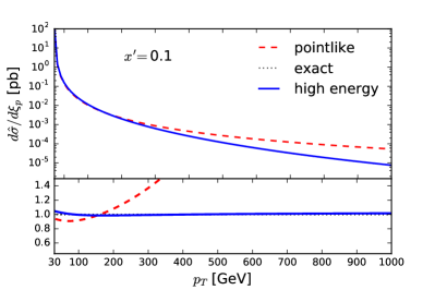
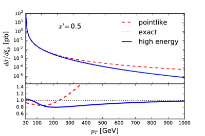
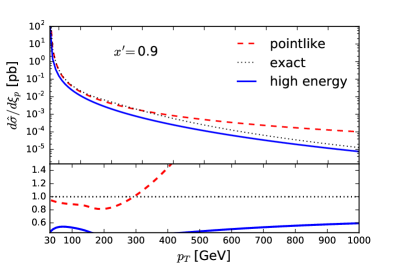
Figure 1: The partonic leading order transverse momentum distribution in the high-energy limit (blue, solid) compared to the exact result of Ref. Baur:1989cm (black, dotted). The leading order pointlike result Ellis:1987xu is also shown for comparison (red, dot-dashed). Results are shown for three different values of $x^{\prime}$ Eq. (2.5): $x^{\prime}=0.01$ (top left), $x^{\prime}=0.1$ (top right), $x^{\prime}=0.5$ (bottom left), $x^{\prime}=0.9$ (bottom right); in each case, the ratio to the exact result is also plotted.

In Figure 1 we compare the exact Baur:1989cm , high-energy and pointlike Ellis:1987xu LO results for four different values of $x^{\prime}$ Eq. (2.5). Here and henceforth we only show predictions for large enough $p_{T}>30$ GeV: at lower $p_{T}$ fixed-order predictions cease to be valid, and must be improved through Sudakov resummation. The relation of the latter to the high-energy approximation was recently discussed in Ref. Marzani:2015oyb . As expected, the pointlike approximation breaks down for $p_{\rm\scriptscriptstyle\rm T}\gtrsim m_{t}$ where the finite-mass result drops rather faster; the deficit which is seen in the pointlike result for $p_{\rm\scriptscriptstyle\rm T}<m_{t}$ is due to the finite bottom mass. The high-energy approximation appears to be very accurate for $x^{\prime}\lesssim 0.1$; for higher $x^{\prime}$ values it starts deteriorating and for large $x^{\prime}\sim 0.5$ it is typically off by 20%. However, the accuracy of the high-energy approximation does not depend on $p_{\rm\scriptscriptstyle\rm T}$ if $p_{\rm\scriptscriptstyle\rm T}\gtrsim m_{H}$: the large-$p_{\rm\scriptscriptstyle\rm T}$ behaviour of the high-energy approximation is qualitatively the same as that of the full result.

The pointlike approximation instead departs from the exact result by an increasingly large amount as $p_{\rm\scriptscriptstyle\rm T}$ grows: in fact, as $p_{\rm\scriptscriptstyle\rm T}\to\infty$, $c_{0}\left(\xi_{p},y_{t},y_{b}\right)$ Eq. (3.3) drops at least as $\frac{1}{p_{\rm\scriptscriptstyle\rm T}^{2}}$, while it is constant in the effective theory, so $\frac{d\sigma^{\text{LL}x-\text{LO}}}{d\xi_{p}}\mathrel{\mathop{\sim}\limits_{\scriptscriptstyle{p_{\rm\scriptscriptstyle\rm T}\rightarrow\infty}}}\frac{1}{\left(p_{\rm\scriptscriptstyle\rm T}^{2}\right)^{a}}$ with $a=2$ in the full theory, and $a=1$ in the effective theory. In the opposite limit $p_{\rm\scriptscriptstyle\rm T}\to 0$ instead, as discussed in Section 2.3 (see Eq. (2.42)), the high-energy limit becomes pointlike, up to an overall rescaling: it is indeed clear from the plots that in the region $x^{\prime}\lesssim 0.1$ in which the high-energy approximation holds, as $p_{\rm\scriptscriptstyle\rm T}\to 0$ the high-energy and pointlike results coincide. An immediate consequence of this discussion is that in the large $p_{\rm\scriptscriptstyle\rm T}\gtrsim m_{t}$ region it is generally rather more advantageous to rely on the high-energy approximation, than use pure effective field theory results, as we will discuss in more detail in Section. 4.

3.2 Expansion coefficients beyond the leading order

We now study the expansion coefficients of the impact factor Eq. (2.3), which we compute including both top and bottom mass, i.e. using Eq. (2.36). As discussed in the end of Sect. 2.3, the LL$x$ transverse momentum distribution up to NNLO is fully determined from knowledge of the first three coefficients. Explicitly, using Eq. (2.3) with Eqs. (2.38-2.39) and inverting the Mellin transform Eq. (2.9) we get

$$\frac{d\sigma}{d\xi_{p}}\left(x,\xi_{p},y_{t},y_{b}\right)=\sigma_{0}\left(y_{t},y_{b}\right)\sum_{k=1}^{\infty}C_{k}\left(\xi_{p},y_{t},y_{b}\right)\alpha_{s}^{k}(-1)^{k+1}\frac{\ln^{k-1}x}{(k-1)!}$$ (3.4)

with

$$C_{1}\left(\xi_{p},y_{t},y_{b}\right) =\frac{2C_{\rm\scriptscriptstyle\rm A}}{\pi}\frac{c_{0}\left(\xi_{p},y_{t},y_{b}\right)}{\xi_{p}}$$ (3.5a)

$$C_{2}\left(\xi_{p},y_{t},y_{b}\right) =\frac{2C_{\rm\scriptscriptstyle\rm A}^{2}}{\pi^{2}}\frac{2c_{0}\left(\xi_{p},y_{t},y_{b}\right)\ln\xi_{p}+c_{1,1}\left(\xi_{p},y_{t},y_{b}\right)}{\xi_{p}}$$ (3.5b)

$$C_{3}\left(\xi_{p},y_{t},y_{b}\right) =\frac{2C_{\rm\scriptscriptstyle\rm A}^{3}}{\pi^{3}}\frac{2c_{0}\left(\xi_{p},y_{t},y_{b}\right)\ln^{2}\xi_{p}+2c_{1,1}\left(\xi_{p},y_{t},y_{b}\right)\ln\xi_{p}+c_{2,1}\left(\xi_{p},y_{t},y_{b}\right)}{\xi_{p}}.$$ (3.5c)

Note that the leading power of $\ln\xi_{p}$ is always proportional to the lowest order coefficient $c_{0}$.

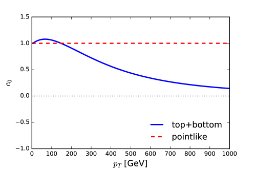
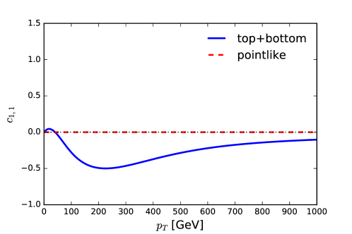
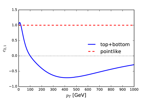
Figure 2: The first three coefficients $c_{i,j}$ Eq. 2.36 in the expansion of the transverse-momentum dependent impact factor Eq. (2.3) with finite top and bottom masses, compared to the pointlike result.

The coefficients are shown in Fig. 2, and compared to their (constant) pointlike counterparts Forte:2015gve . As expected, the coefficients tend to the pointlike limit as $\xi_{p}\to 0$, while they vanish at large $\xi_{p}$, as required in order for the inclusive cross-section to be free of spurious double energy logs, as discussed in Ref. Forte:2015gve . In the high-energy limit, the overall power behaviour at large $p_{T}$ remains the same to all orders, and equal to that of the leading order, which as we have seen above, coincides with theat of the exact leading order. The fact that the high-energy approximation holds as $x^{\prime}\to 1$, while in the opposite $x^{\prime}\to 1$ limit the high-$p_{\rm\scriptscriptstyle\rm T}$ power behaviour is also to all orders the same of the leading-order result deFlorian:2005fzc suggests that the high-energy approximation reproduces the correct high-$p_{T}$ behaviour of the full result to all orders.

As seen in Sect. 3.1, the pointlike approximation breaks down for $p_{\rm\scriptscriptstyle\rm T}\sim m_{t}$. In the high-energy limit, one expects the departure from pointlike to become increasingly marked as the perturbative order is raised, because with an increasingly large number of hard emissions more energy flows into the loop which is less well approximated by a pointlike interaction: so higher-order coefficients $c_{i,j}$ deviate more from their pointlike limit than lower-order ones. On the other hand, the lower order coefficients are enhanced by higher powers of $\ln\xi_{p}$, see Eqs.(3.4-3.5), so low-order coefficients dominate, and the shape of the $p_{\rm\scriptscriptstyle\rm T}$ distribution remains similar as the perturbative order is increased, as we will also discuss at the hadronic level in Sect. 4.

Also as discussed in Sect. 3.1, the effect of the bottom quark can be seen in the departure of the coefficients from the pointlike value at small $p_{\rm\scriptscriptstyle\rm T}$, even though the pointlike limit is always recovered in the $p_{\rm\scriptscriptstyle\rm T}\to 0$ limit. It is interesting to assess the relative impact of the bottom, top, and interference contributions. In order to do this, we write each coefficient as

$$c_{j,k}\left(\xi_{p},y_{t},y_{b}\right)=R^{\rm t}\left(y_{t},y_{b}\right)\>c_{j,k}^{\rm t}\left(\xi_{p},y_{t}\right)+R^{\rm b}\left(y_{t},y_{b}\right)\>c_{j,k}^{\rm b}\left(\xi_{p},y_{b}\right)+R^{\rm i}\left(y_{t},y_{b}\right)\>c_{j,k}^{\rm i}\left(\xi_{p},y_{t},y_{b}\right),$$ (3.6)

where the normalization ratios

$$R^{\rm t}\left(y_{t},y_{b}\right) =\frac{\left|\,K(y_{t})\,\right|^{2}}{\left|\,K(y_{t})+K(y_{b})\,\right|^{2}}=1.107$$ (3.7a)

$$R^{\rm b}\left(y_{t},y_{b}\right) =\frac{\left|\,K(y_{b})\,\right|^{2}}{\left|\,K(y_{t})+K(y_{b})\,\right|^{2}}=0.008$$ (3.7b)

$$R^{\rm i}\left(y_{t},y_{b}\right) =\frac{K(y_{b})^{*}K(y_{t})+K(y_{b})K(y_{t})^{*}}{\left|\,K(y_{t})+K(y_{b})\,\right|^{2}}=-0.115.$$ (3.7c)

account for the mismatch in normalization between the Wilson coefficients $K$ in the form factor Eq. (2.27) when both the top and bottom contributions are included.

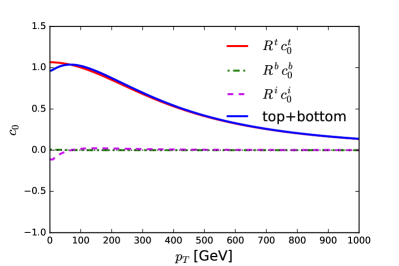
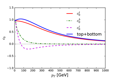
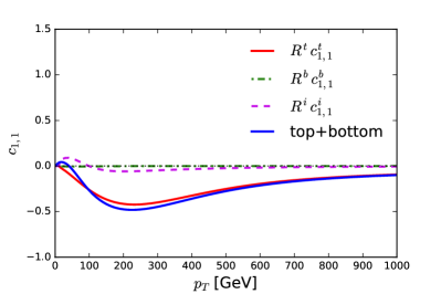
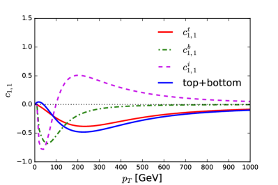
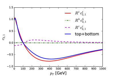
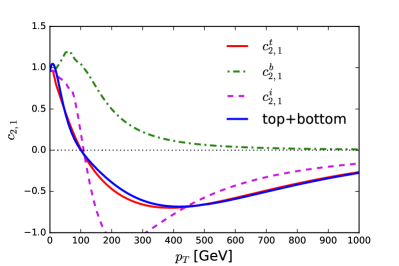
Figure 3: Contribution from top (red, solid), bottom (green, dot-dashed) and interference (purple, dashed) to the coefficients shown in Fig. 2, with their sum also shown as blue line: the three coefficients $c_{0}$, $c_{1,1}$ and $c_{2,1}$ are shown from top to bottom, including (left) or not including (right) the normalization due to the Wilson coefficient Eqs. (3.6-3.7).

The separate contributions are compared in Fig. 3 to each other and to their sums, already shown in Fig. (2), both with and without the normalization coefficients Eq. (3.7). It is clear that while in each case the un-normalized coefficients $c^{\rm t}$, $c^{\rm b}$ and $c^{\rm i}$ are all of the same order, after multiplying by the Wilson coefficients Eqs. (3.7) the top contribution is dominant, while the pure bottom contribution becomes entirely negligible. However, in the region $m_{b}\lesssim p_{\rm\scriptscriptstyle\rm T}\lesssim m_{t}$ and even for somewhat larger $p_{\rm\scriptscriptstyle\rm T}$ values the interference contribution provides a small but non-negligible correction. Fig. 3 shows that this feature, well known at LO, appears to persist also at higher orders. In this range of $p_{\rm\scriptscriptstyle\rm T}$, the transverse momentum spectrum acquires a dependence on $\ln\frac{p_{\rm\scriptscriptstyle\rm T}^{2}}{m_{b}^{2}}$, as we now discuss.

3.3 Bottom Logs

The region in which $m_{b}\lesssim p_{\rm\scriptscriptstyle\rm T}\lesssim m_{t}$ is particularly intricate because the Higgs momentum spectrum becomes a multi-scale problem. Indeed, it was pointed out in Ref. Bagnaschi:2011tu that in this region finite bottom mass effect are visible in the spectrum, which thus deviates from the prediction obtained using transverse momentum resummation. Specifically, in Ref. Banfi:2013eda it was shown that the cross-section contains contributions proportional to $\ln\frac{p_{\rm\scriptscriptstyle\rm T}^{2}}{m_{b}^{2}}$ which can be traced to non-factorized soft or collinear logs. This immediately raises the question whether such behaviour persists at higher orders, perhaps requiring resummation Banfi:2013eda ; Grazzini:2013mca ; Bagnaschi:2015qta . The resummation of these soft logs as recently discussed in Ref. Melnikov:2016emg ; in the high energy limit considered here we focus on the collinear ones instead.

It turns out in fact that, in the high-energy limit, collinear logs are present to all perturbative orders, but not of increasingly high logarithmic order, at least at the LL$x$ level. To see this, we first consider our LO result Eq. (3.3) when $m_{b}^{2}<p_{\rm\scriptscriptstyle\rm T}^{2}<m_{h}^{2}$ Banfi:2013eda , i.e., using dimensionless variables $y_{b}<\xi_{p}<1$. Collinear bottom mass logs are extracted by performing the simultaneous limit $\frac{y_{b}}{\xi_{p}}\to 0$ and $\xi_{p}\to 0$ Banfi:2013eda . We get

$$\frac{d\sigma^{LO}}{d\xi_{p}}\left(x,\xi_{p},y_{b}\right)\mathrel{\mathop{\sim}\limits_{\scriptscriptstyle{y_{b}\rightarrow 0}}}\frac{G_{\scriptscriptstyle\rm F}\sqrt{2}\alpha_{s}^{2}}{256\pi^{2}}\frac{2C_{\rm\scriptscriptstyle\rm A}\alpha_{s}}{\pi\xi_{p}}y_{b}^{2}\left|\,\ln^{2}\frac{\xi_{p}}{y_{b}}-\ln^{2}\left(-y_{b}\right)+4\,\right|^{2}.$$ (3.8)

But $\frac{\xi_{p}}{y_{b}}=\frac{p_{\rm\scriptscriptstyle\rm T}^{2}}{m^{2}_{b}}$, so this agrees with the conclusion of Ref. Banfi:2013eda that the transverse momentum spectrum contains a collinear contribution proportional to $\frac{m_{b}^{4}}{p_{\rm\scriptscriptstyle\rm T}^{2}m_{H}^{2}}\ln^{4}\frac{p_{\rm\scriptscriptstyle\rm T}^{2}}{m^{2}_{b}}$.

The corresponding result at all orders can be obtained by performing the same limit on the function $F$ Eq. (2.27), which contains all the $\xi_{p}$ and $y_{b}$ dependence of the resummed result. We get

$$F\left(\xi_{1},\xi_{2},\xi_{p},y_{b}\right)\mathrel{\mathop{\sim}\limits_{\scriptscriptstyle{y_{b}\rightarrow 0}}}\Bigg{[}p_{4}\left(\xi_{1},\xi_{2}\right)\ln^{4}\frac{\xi_{p}}{y_{b}}+p_{3}\left(\xi_{1},\xi_{2}\right)\ln^{3}\frac{\xi_{p}}{y_{b}}\\ +p_{2}\left(\xi_{1},\xi_{2}\right)\ln^{2}\frac{\xi_{p}}{y_{b}}+p_{1}\left(\xi_{1},\xi_{2}\right)\ln\frac{\xi_{p}}{y_{b}}+p_{0}\Bigg{]},$$ (3.9)

where the coefficient of the highest log has the simple form

$$p_{4}\left(\xi_{1},\xi_{2}\right)=\frac{\left(1-\xi_{1}-\xi_{2}\right)^{2}}{4\xi_{1}\xi_{2}},$$ (3.10)

and we omit the lengthy expressions of the other coefficients. Using Eq. (3.10) in Eq. (2.27) the integrals over $\xi_{i}$ in the expression of the coefficients can be performed analytically, and we find that the leading contribution to the impact factor in the limit is

$$h_{p_{\rm\scriptscriptstyle\rm T}}\left(N,M_{1},M_{2},\xi_{p},y_{b}\right)\mathrel{\mathop{\sim}\limits_{\scriptscriptstyle{y_{b}\rightarrow 0}}} \sigma^{\rm PL}_{0}R\left(M_{1}\right)R\left(M_{2}\right)\frac{\xi_{p}^{M_{1}+M_{2}-1}}{\left(1+\xi_{p}\right)^{N}}$$

$$\left[c^{\rm PL}_{0}\left(M_{1}+M_{2}\right)+\sum_{j>k>0}c_{j,k}^{\rm PL}\left(M_{1}^{j}M_{2}^{k}+M_{1}^{k}M_{2}^{j}\right)\right]\ln^{4}\frac{\xi_{p}}{y_{b}},$$ (3.11)

where $c_{i,y}^{\rm PL}$ are the coefficients which appear in the expression of the impact factor in the pointlike limit Eq. (2.3).

Equation (3.3) thus indeed shows that at LL$x$ level a collinear log appears to all orders, but with a fixed power: to all orders at LL$x$ the highest power of log is four. The log originates from the dynamics of the quark loop, but it is to all orders proportional to the pointlike result. Because the highest power of the $\ln p_{\rm\scriptscriptstyle\rm T}^{2}/m_{b}^{2}$ terms is fixed at LL$x$, from our result we cannot exclude higher order logs and their exponentiation at the subleading log-$x$ level.

4 Phenomenology

We now turn to the phenomenological implications of our results. First, we repeat the comparisons that were presented in the previous section at the hadronic level. In particular, we validate the high-energy approximation at leading and next-to-leading order, and then provide prediction for the transverse momentum distribution at NLO based on the high-energy approximation.

As explained in Sect. 3.1, the high-energy approximation is mostly relevant in the region $p_{\rm\scriptscriptstyle\rm T}>m_{H}$, where the pointlike approximation fails, while for lower $p_{\rm\scriptscriptstyle\rm T}$ values the high-energy result rapidly approaches its pointlike limit, and eventually, for low enough $p_{\rm\scriptscriptstyle\rm T}$, Sudakov resummation of transverse momentum logs becomes necessary. In the region of interest for this study, as demonstrated in Sect. 3.2, the contribution of the bottom quark is entirely negligible. Therefore, in the remainder of this section we will only include the top contribution. Furthermore, as previously mentioned, the LL$x$ behaviour of all partonic channels can be deduced from the gluon-gluon case, and will thus be included throughout this section. All plots are produced with $\mu_{\rm\scriptscriptstyle\rm R}^{2}=\mu_{\rm\scriptscriptstyle\rm F}^{2}=Q^{2}$ and with the PDF4LHC15 NNLO set of parton distributions PDF4LHC15_nnlo_100 Butterworth:2015oua ; Ball:2014uwa ; Harland-Lang:2014zoa ; Dulat:2015mca ; Carrazza:2015aoa ; Gao:2013bia ; Watt:2012tq , for the LHC with $\sqrt{s}=13$ TeV.

4.1 Validation of the high-energy approximation

We have seen in Sect. 3.1 that the pointlike approximation to the exact result of Ref. Baur:1989cm deteriorates by an increasingly large amount as $p_{\rm\scriptscriptstyle\rm T}$ grows beyond $p_{\rm\scriptscriptstyle\rm T}\gtrsim m_{H}$, while the high-energy approximation has an accuracy which is essentially independent of $p_{\rm\scriptscriptstyle\rm T}$ for fixed value of the partonic scaling variable $x^{\prime}$ Eq. (2.5). The partonic $x^{\prime}$ is of course bounded by the hadronic $\tau^{\prime}$ Eq. (2.3), which in turn depends on the scale $Q^{2}$ Eq. (2.4) which for large $p_{\rm\scriptscriptstyle\rm T}$ is $Q^{2}\sim\frac{4p_{\rm\scriptscriptstyle\rm T}^{2}}{s}$. Because we have seen that the high-energy approximation is good for $x^{\prime}\lesssim 0.5$ and only deteriorates slowly for larger values of $x^{\prime}$, noting that $\tau^{\prime}=0.5$ corresponds to $p_{\rm\scriptscriptstyle\rm T}\sim 4.6$ TeV for the LHC at 13 TeV, we expect the high-energy approximation to be reasonably accurate up to large values of $p_{\rm\scriptscriptstyle\rm T}$.

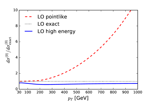
Figure 4: The ratio of the high-energy approximation (in solid blue) and of the effective theory result (in dotted red) to the full result for the hadron-level transverse momentum distribution at LO plotted as a function of $p_{\rm\scriptscriptstyle\rm T}$ (GeV) at the LHC 13 TeV.

We define the NLO transverse momentum distribution

$$\frac{d\sigma}{d\xi_{p}}\left(\tau^{\prime},\xi_{p},y_{t},\alpha_{s}\right)=\alpha_{s}\frac{d\sigma^{(0)}}{d\xi_{p}}+\alpha_{s}^{2}\frac{d\sigma^{(1)}}{d\xi_{p}}+\mathcal{O}\left(\alpha_{s}^{3}\right),$$ (4.1)

and the $K$-factor

$$K=1+\frac{d\sigma^{(1)}/d\xi_{p}}{d\sigma^{(0)}/d\xi_{p}}.$$ (4.2)

In Figure 4 we compare the leading order contribution $\frac{d\sigma^{(0)}}{d\xi_{p}}$ computed in the high-energy approximation to the exact result of Ref. Baur:1989cm , and also with the effective-field theory result. It is clear that, as expected, the high-energy approximation is most accurate for $p_{\rm\scriptscriptstyle\rm T}\sim m_{H}$ but only slowly deteriorates for larger $p_{\rm\scriptscriptstyle\rm T}$: in fact, for all $0.5\lesssim p_{\rm\scriptscriptstyle\rm T}\lesssim 1$ TeV the high-energy approximation is about 60% of the full theory LO result. The effective field theory result instead is driven by the fact that at the parton level it has the wrong large-$p_{\rm\scriptscriptstyle\rm T}$ power behaviour, and is off by an increasingly large factor: at $p_{\rm\scriptscriptstyle\rm T}\sim 1$ TeV it is in fact too large by about one order of magnitude.

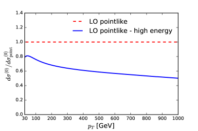
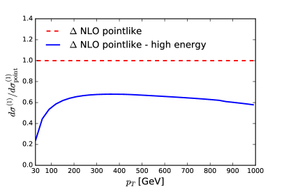
Figure 5: The ratio of the high-energy approximation to the pointlike result for the hadron-level transverse momentum distribution plotted as a function of $p_{\rm\scriptscriptstyle\rm T}$ (GeV) at the LHC 13 TeV for the LO, on the left and for the NLO contribution, on the right.

Beyond leading order we do not have any exact result to compare to, as only the effective field theory result is available. We expect a similar pattern to hold, and we can provide some evidence for this by studying the relation between the high-energy approximation and the full result, both determined in the pointlike limit. This comparison is shown in Fig. 5 (left) for the LO contribution $\frac{d\sigma^{(0)}}{d\xi_{p}}$. It is apparent that the quality of the high-energy approximation in the pointlike limit is quite similar to that in the full theory discussed above. The NLO contribution $\frac{d\sigma^{(1)}}{d\xi_{p}}$ is also shown in Fig. 5 (right): we compare the high-energy pointlike result of Ref. Forte:2015gve to the full result of Ref. Glosser:2002gm . Again, in the medium-high $p_{\rm\scriptscriptstyle\rm T}$ region we are interested in the pattern is quite similar to that seen at LO.

This suggests that the high-energy approximation might remain accurate in a relatively wide kinematic region. In order to test this, we have repeated the comparison of the high-energy to the full result for the NLO term $\frac{d\sigma^{(1)}}{d\xi_{p}}$ , both in the pointlike limit, shown in Fig. 5, for a wide range of values of $p_{\rm\scriptscriptstyle\rm T}$ and the collider energy. Results are shown in Fig. 6. As expected, the high-energy approximation becomes better as the center-of-mass energy is increased at fixed $p_{\rm\scriptscriptstyle\rm T}$. On the other hand, if $p_{\rm\scriptscriptstyle\rm T}$ is varied at fixed energy the quality of the approximation remains constant in a wide range of transverse momenta, and it only starts deteriorating when the transverse momentum is larger than say $\sim 20\%$ of its upper kinematic limit $\sqrt{s}/2$. This is expected because the high-energy limit holds when $\sqrt{s}$ is much larger than all other scales: for instance, at large $p_{\rm\scriptscriptstyle\rm T}$ there are $\ln p_{\rm\scriptscriptstyle\rm T}$ contributions which should be resummed to all orders Berger:2001wr , but are increasingly subleading in the high-energy expansion. However, in this region the transverse momentum distribution is tiny, so in practice the high-energy approximation is uniformly accurate throughout the physically relevant region.

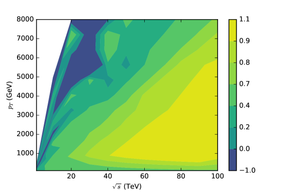
Figure 6: The ratio of the NLO contribution $\frac{d\sigma^{(1)}}{d\xi_{p}}$ in the high-energy approximation to exact result, both computed in the pointlike limit, for the Higgs transverse momentum distribution at a proton-proton collider plotted as a function of the transverse momentum $p_{\rm\scriptscriptstyle\rm T}$ (in GeV) and the center-of-mass energy $\sqrt{s}$ (in TeV).

4.2 The mass-dependent spectrum beyond leading order

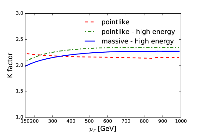
Figure 7: The NLO $K$-factor Eq. (4.2) computed using the full result in the pointlike limit (red, dashed), and the high-energy approximation, either with full mass dependence (blue, solid) or in the pointlike limit (green, dotdashed). In each case, the LO cross-section is computed using the same approximation as the NLO term.

We now finally turn to the $p_{\rm\scriptscriptstyle\rm T}$ spectrum of the Higgs boson with finite top mass beyond leading order. In this case the exact result is unknown, and thus we can only compare different approximations. In Fig. 7 we compare three different determinations of the $K$-factor Eq. (4.2) in the high-$p_{\rm\scriptscriptstyle\rm T}$ region we are interested in: using the full pointlike NLO result, the high-energy approximation to it (i.e. pointlike, and high-energy), and the high-energy result, but with full mass dependence. In each case, both the LO and NLO contributions are computed using the same approximation. This plot shows that for $p_{\rm\scriptscriptstyle\rm T}\gtrsim 200$ GeV all these $K$-factors have a similar behaviour, and differ by comparable amounts.

This plot suggests two main conclusions. First, in the only case in which we can compare the high-energy approximation to the full result, namely the pointlike limit, we see that the high-energy approximation is quite good (red vs. green curve in Fig. 7), with an accuracy of about 20% or better for all $p_{\rm\scriptscriptstyle\rm T}\gtrsim 200$ GeV, which does not deteriorate as $p_{\rm\scriptscriptstyle\rm T}$ increases. Second, even though (recall Sect. 3) the shape of the distribution at high $p_{\rm\scriptscriptstyle\rm T}$ differs between the pointlike and massive case (a different power of $p_{\rm\scriptscriptstyle\rm T}$) the $K$ factors are similar and approximately $p_{\rm\scriptscriptstyle\rm T}$ independent, at least in the only case in which we can compare the pointlike and massive results, namely the high-energy limit (green and blue curve).

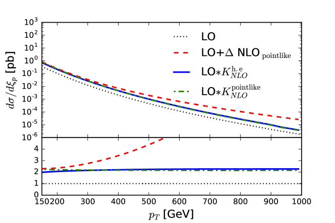
Figure 8: Various approximations to the NLO Higgs transverse momentum distribution. The curves shown correspond (from top to bottom) to adding the pointlike approximation to the NLO contribution to the full LO result (red, dashed), or to multiplying the full LO result by the $K$-factors of Fig. (7) computed respectively in the high-energy approximation but with full mass dependence (blue, solid) or in the pointlike approximation (green dot-dashed). The full LO result is also shown for comparison (black, dotted). In the bottom plot all curves are shown as ratios to the exact LO result.

These two observations, taken together, suggest that the best approximation to the full NLO result can be obtained by combining the full LO result with a $K$-factor computed in the high-energy approximation, namely, by multiplying the LO cross-section by the $K$ factor (blue curve) of Fig. 7, corresponding to the high-energy fully massive result. This is our preferred approximation, and it is shown in Fig. 8, where it is also compared to the LO exact result and to the NLO pointlike approximation; all results are also shown as ratios to the LO. It is clear that the pointlike result has the wrong power behaviour at large $p_{\rm\scriptscriptstyle\rm T}$ and thus fails for $p_{\rm\scriptscriptstyle\rm T}\gtrsim 200$ GeV.

The comparison of $K$-factors of Fig. 7 suggests that if one wishes to use the NLO pointlike result, rather than the high-energy approximation, a better approximation can be obtained by using the pointlike NLO to compute the $K$ factor (red curve of Fig. 7), and using this $K$ factor to rescale the full massive leading order. The quality of this approximation is possibly comparable to that of our favorite approximation based on the high-energy limit: indeed, as discussed in Sect. 3.2 this approximation captures the leading log contributions proportional to $c_{0}$ in Eq. (3.5). This curve is also shown in Fig. 8: it is seen to be quite close to our favorite approximation in a wide range of $p_{\rm\scriptscriptstyle\rm T}$ but it starts departing from it only at the largest $p_{\rm\scriptscriptstyle\rm T}$ where we expect the high-energy approximation to be more accurate.

If our approximation to the $K$-factor based on the high-energy limit is used, it is natural to ask what is the associated uncertainty. Having observed that, at the level of $K$-factors, the difference between the pointlike and massive cases is somewhat smaller than the difference between the high-energy and full results (see Fig. 8), we can conservatively estimate the uncertainty on the high-energy approximation to be given by the percentage discrepancy between high-energy and full results (both pointlike) shown in Fig. 6. Of course, this is just the uncertainty related to the high-energy approximation, which will then have to be supplemented with all other sources of uncertainty (missing higher orders, $\alpha_{s}$, PDFs, etc.).

Before concluding, let us comment on different approaches that can be found in the literature. So far studies of finite top mass effects have been performed by merging different hard-jet multiplicities and parton showers Buschmann:2014sia and, more recently, in Ref. Frederix:2016cnl and in the context of jet veto analysis Banfi:2013eda and NNLO matching to parton showers Hamilton:2015nsa .

In Refs. Harlander:2012hf ; Neumann:2014nha , finite top mass effects were evaluated using an asymptotic expansion in inverse powers of the top mass. This expansion is accurate below $2m_{t}$ and finite-top mass corrections in this region were found to below 10%. Our approximation, which is valid in the high-$p_{\rm\scriptscriptstyle\rm T}$ region, is therefore complementary and one would expect that a combination of the two approaches, in analogy to what was done for the inclusive case Harlander:2009my ; Pak:2009dg , will provide a reliable approximation across a wide range of $p_{\rm\scriptscriptstyle\rm T}$.

In Ref. Buschmann:2014sia , top mass effects on the transverse momentum distribution were calculated using a matched parton shower approach. This analysis is particularly interesting for us because both the approach of Ref. Buschmann:2014sia and ours implicitly relies on the assumption that real radiation provides the bulk of radiative corrections in the high $p_{\rm\scriptscriptstyle\rm T}$ region. Nevertheless, this assumption is then used quite differently in the merged sample and high-energy approximations. Indeed, in the former real emission diagrams are accounted for exactly, while virtual corrections are dropped altogether. The final result is then affected by merging ambiguities. In the high-energy approach instead real emission is only included in the LL$x$ approximation, accompanied however by a matching set of virtual corrections to ensure a well-defined NLO result.

Despite these differences, both approaches are supposed to capture the bulk of NLO corrections in the high $p_{\rm\scriptscriptstyle\rm T}$ region, where the dominance of real emission is a reasonable assumption. As a consequence, a significant disagreement between our results and Ref. Buschmann:2014sia would imply the presence of large out of control subleading effects, which would somewhat hamper the phenomenological relevance of these analysis. Fortunately, it turns out that the two approaches lead instead to the same conclusions. Indeed, in the high transverse momentum region we find that the $K$ factor in the pointlike and exact theory are comparable, and that the shape in $p_{\rm\scriptscriptstyle\rm T}$ of our NLO approximation closely follows the behaviour of exact LO, in agreement with conclusion drawn with the analysis of Ref. Buschmann:2014sia (see for example Fig. $4$ of that reference).

5 Conclusion

In this paper, we have applied the high-energy resummation of transverse momentum distributions of Ref. Forte:2015gve to Higgs production in gluon fusion with full dependence on heavy quark masses. We have determined explicit expressions for the resummation coefficients of the resummed results to all orders.

The all-order expression has enabled us to show that the collinear bottom mass logs which are relevant in the region $m_{b}<p_{\rm\scriptscriptstyle\rm T}<m_{H}$ are present to all orders in the high-energy limit, but with a fixed power of log. We have then studied the impact of finite mass corrections in the first few orders. We have shown that the pointlike approximation fails badly for $p_{\rm\scriptscriptstyle\rm T}\gtrsim m_{t}$, while the high-energy approximation provides reasonably accurate results for center-of-mass energies above a few TeV and for all $p_{\rm\scriptscriptstyle\rm T}$. Its accuracy does not deteriorate as $p_{\rm\scriptscriptstyle\rm T}$ grows, unless $p_{\rm\scriptscriptstyle\rm T}$ becomes a sizable fraction of the center-of-mass energy.

We have thus argued that the best approximation to the transverse momentum distribution at past and future LHC energies for all $p_{\rm\scriptscriptstyle\rm T}\gtrsim 200$ GeV can be obtained by combining the known exact leading order result with a $K$-factor computed in the high-energy approximation. At the hadronic level, we have provided results to NLO; the partonic NNLO results presented here suggest that it will be interesting to investigate the relative accuracy of various approximations at NNLO and beyond. More accurate approximations to the full result could be constructed by combining information on the $p_{\rm\scriptscriptstyle\rm T}$ distribution coming from the high-energy limit with that from the opposite soft limit, in which resummed results are also available deFlorian:2005fzc . All these developments are under investigation and will be the object of forthcoming publications.

Appendix A Form factors and perturbative coefficients

We give here the expressions used in the computation of the $p_{\rm\scriptscriptstyle\rm T}$-impact factor presented in Sect. 2. We also provide analytic form of the first LO coefficient of the expansion in power of $\alpha_{s}$ of the $p_{\rm\scriptscriptstyle\rm T}$-impact factor, discussed in Sect. 3.1.

The $p_{\rm\scriptscriptstyle\rm T}$-impact factor is expressed in Eq. (2.2) as a double integral over $\xi_{1}$ and $\xi_{2}$ of a function $F\left(\xi_{1},\xi_{2},\xi_{p},\{y_{i}\}\right)$. This function is deduced from the off-shell form factor $\tilde{F}\left(\xi,\bar{\xi},\xi_{p},\{y_{i}\}\right)$ as

$$F\left(\xi_{1},\xi_{2},\xi_{p},\{y_{i}\}\right)=\tilde{F}\left(\xi_{p}\,\xi_{1},\xi_{p}\,\xi_{2},\xi_{p},\{y_{i}\}\right).$$ (A.1)

This form factor is given by DelDuca:2001fn ; Marzani:2008az :

$$\tilde{F}\left(\xi,\bar{\xi},\xi_{p},\{y_{i}\}\right)=\frac{2304\pi^{4}}{\left|\,\sum_{i}K\left(y_{i}\right)\,\right|^{2}}\left|\,\sum_{i}y_{i}\,A\left(\xi,\bar{\xi},\xi_{p},y_{i}\right)\,\right|^{2}$$ (A.2)

with the sum $i$ which runs over the set $\{y_{i}\}$ of quarks circulating in the loop, and

$$A\left(\xi,\bar{\xi},\xi_{p},y\right)=\frac{C_{0}\left(\xi,\bar{\xi},y\right)}{\sqrt{\xi\bar{\xi}}}$$

$$\Bigg{[}\left(\frac{2y}{\Delta_{3}}+\frac{6\xi\bar{\xi}}{\Delta_{3}^{2}}\right)\left(\left(\xi_{p}-\xi-\bar{\xi}\right)\left(1+\xi+\bar{\xi}\right)+4\xi\bar{\xi}\right)-\frac{\xi_{p}-\xi-\bar{\xi}}{2}+2\frac{\xi\bar{\xi}\left(1-\xi_{p}\right)}{\Delta_{3}}\Bigg{]}$$

$$-\frac{1}{\sqrt{\xi\bar{\xi}}}\left[B_{0}\left(-\bar{\xi},y\right)-B_{0}\left(1,y\right)\right]\left[-\frac{\bar{\xi}}{\Delta_{3}}\left(\xi_{p}-\bar{\xi}+\xi\right)+\frac{6\xi\bar{\xi}}{\Delta_{3}^{2}}\left(1+\xi_{p}\right)\left(1+\xi-\bar{\xi}\right)\right]$$

$$-\frac{1}{\sqrt{\xi\bar{\xi}}}\left[B_{0}\left(-\xi,y\right)-B_{0}\left(1,y\right)\right]\left[-\frac{\xi}{\Delta_{3}}\left(\xi_{p}-\xi+\bar{\xi}\right)+\frac{6\xi\bar{\xi}}{\Delta_{3}^{2}}\left(1+\xi_{p}\right)\left(1+\bar{\xi}-\xi\right)\right]$$

$$+\frac{1}{4\pi^{2}}\frac{1}{\Delta_{3}}\frac{1}{\sqrt{\xi\bar{\xi}}}\left(\left(\xi_{p}-\xi-\bar{\xi}\right)\left(1+\xi+\bar{\xi}\right)+\xi\bar{\xi}\right)$$ (A.3)

where $\Delta_{3}=\left(1+\xi+\bar{\xi}\right)^{2}-4\xi\bar{\xi}$ and

$$B_{0}\left(\rho,y\right) =-\frac{1}{16\pi^{2}}\sqrt{\frac{\rho-4y}{\rho}}\ln\frac{\sqrt{\frac{\rho-4y}{\rho}}+1}{\sqrt{\frac{\rho-4y}{\rho}}-1}$$ (A.4)

$$C_{0}\left(\xi,\bar{\xi},y\right) =\frac{1}{16\pi^{2}}\frac{1}{\sqrt{\Delta_{3}}}\Bigg{[}\ln\left(1-y_{-}\right)\ln\left(\frac{1-y_{-}\delta_{1}^{+}}{1-y_{-}\delta_{1}^{-}}\right)$$

$$+\ln\left(1-x_{-}\right)\ln\left(\frac{1-x_{-}\delta_{2}^{+}}{1-x_{-}\delta_{2}^{-}}\right)+\ln\left(1-z_{-}\right)\ln\left(\frac{1-z_{-}\delta_{3}^{+}}{1-z_{-}\delta_{3}^{-}}\right)$$

$$+\mathrm{Li}_{2}\left(y_{+}\delta_{1}^{+}\right)+\mathrm{Li}_{2}\left(y_{-}\delta_{1}^{+}\right)-\mathrm{Li}_{2}\left(y_{+}\delta_{1}^{-}\right)-\mathrm{Li}_{2}\left(y_{-}\delta_{1}^{-}\right)$$

$$+\mathrm{Li}_{2}\left(x_{+}\delta_{2}^{+}\right)+\mathrm{Li}_{2}\left(x_{-}\delta_{2}^{+}\right)-\mathrm{Li}_{2}\left(x_{+}\delta_{2}^{-}\right)-\mathrm{Li}_{2}\left(x_{-}\delta_{2}^{-}\right)$$

$$+\mathrm{Li}_{2}\left(z_{+}\delta_{3}^{+}\right)+\mathrm{Li}_{2}\left(z_{-}\delta_{3}^{+}\right)-\mathrm{Li}_{2}\left(z_{+}\delta_{3}^{-}\right)-\mathrm{Li}_{2}\left(z_{-}\delta_{3}^{-}\right)\Bigg{]}$$ (A.5)

with

$$\delta_{1} \equiv\frac{-\xi+\bar{\xi}-1}{\sqrt{\Delta_{3}}}, \delta_{2} \equiv\frac{\xi-\bar{\xi}-1}{\sqrt{\Delta_{3}}}, \delta_{3} \equiv\frac{\xi+\bar{\xi}+1}{\sqrt{\Delta_{3}}},$$ (A.6)

$$\delta_{i}^{\pm} \equiv\frac{1\pm\delta_{i}}{2},$$ (A.7)

and

$$x_{\pm} \equiv-\frac{\bar{\xi}}{2y}\Bigg{(}1\pm\sqrt{1+\frac{4y}{\bar{\xi}}}\Bigg{)},$$ (A.9)

$$y_{\pm} \equiv-\frac{\xi}{2y}\Bigg{(}1\pm\sqrt{1+\frac{4y}{\xi}}\Bigg{)},$$ (A.10)

$$z_{\pm} \equiv\frac{1}{2y}\Bigg{(}1\pm\sqrt{1-4y}\Bigg{)}.$$ (A.11)

The form factor $A$ can be expressed in terms of standard one-loop scalar integrals Ellis:2007qk by letting $C_{0}(\xi,\bar{\xi},y_{i})=m_{h}^{2}I_{3}(-\xi m_{h}^{2},-\bar{\xi}m_{h}^{2},m_{h}^{2},m_{i}^{2},m_{i}^{2},m_{i}^{2})/(16\pi^{2})$ and $B_{0}(\rho,y)-B_{0}(1,y)=\left[I_{2}(\rho m_{h}^{2},m_{i}^{2},m_{i}^{2})-I_{2}(m_{h}^{2},m_{i}^{2},m_{i}^{2})\right]/(16\pi^{2})$. As already stated in the main text, the analytic continuation of the form factor has to be handled by giving $y$ a small negative imaginary part.

Using these expressions, we obtain the following limiting cases

$$\lim_{y\to\infty}F\left(\xi_{1},\xi_{2},\xi_{p},y\right) =\frac{\left(1-\xi_{1}-\xi_{2}\right)^{2}}{4\xi_{1}\xi_{2}}$$ (A.12)

$$\lim_{\xi_{p}\to 0}F\left(\xi_{1},\xi_{2},\xi_{p},\{y_{i}\}\right) =\frac{\left(1-\xi_{1}-\xi_{2}\right)^{2}}{4\xi_{1}\xi_{2}}.$$ (A.13)

Finally, we provide an analytic expression for the first expansion coefficient $c_{0}$ Eq. (2.36) of the perturbative expansion Eq. (2.3):

$$c_{0}\left(\xi_{p},\{y_{i}\}\right)=\frac{2304\pi^{4}}{\left|\,\sum_{i}K\left(y_{i}\right)\,\right|^{2}}\left|\,\sum_{i}y_{i}\,A\left(0,\xi_{p},\xi_{p},y_{i}\right)\,\right|^{2}$$ (A.14)

with

$$A\left(0,\xi_{p},\xi_{p},y\right) =\frac{1}{32\pi^{2}}\Bigg{(}\frac{4y-1-\xi_{p}}{\left(1+\xi_{p}\right)^{2}}\Bigg{[}\ln^{2}\frac{\sqrt{1-4y}-1}{\sqrt{1-4y}+1}-\ln^{2}\frac{\sqrt{1+\frac{4y}{\xi_{p}}}-1}{\sqrt{1+\frac{4y}{\xi_{p}}}+1}\Bigg{]}$$

$$+\frac{4\xi_{p}}{\left(1+\xi_{p}\right)^{2}}\Bigg{[}\sqrt{1-4y}\ln\frac{\sqrt{1-4y}+1}{\sqrt{1-4y}-1}-\sqrt{1+\frac{4y}{\xi_{p}}}\ln\frac{\sqrt{1+\frac{4y}{\xi_{p}}}+1}{\sqrt{1+\frac{4y}{\xi_{p}}}-1}\Bigg{]}$$

$$+\frac{4}{1+\xi_{p}}\Bigg{)}.$$ (A.15)

References

- (1) ATLAS Collaboration, G. Aad et al., Observation of a new particle in the search for the Standard Model Higgs boson with the ATLAS detector at the LHC, Phys. Lett. B716 (2012) 1–29, [arXiv:1207.7214].
- (2) CMS Collaboration, S. Chatrchyan et al., Observation of a new boson at a mass of 125 GeV with the CMS experiment at the LHC, Phys. Lett. B716 (2012) 30–61, [arXiv:1207.7235].
- (3) ATLAS Collaboration, G. Aad et al., Measurements of the Higgs boson production and decay rates and coupling strengths using pp collision data at and 8 TeV in the ATLAS experiment, Eur. Phys. J. C76 (2016), no. 1 6, [arXiv:1507.04548].
- (4) CMS Collaboration, V. Khachatryan et al., Precise determination of the mass of the Higgs boson and tests of compatibility of its couplings with the standard model predictions using proton collisions at 7 and 8 TeV, Eur. Phys. J. C75 (2015), no. 5 212, [arXiv:1412.8662].
- (5) C. Arnesen, I. Z. Rothstein, and J. Zupan, Smoking Guns for On-Shell New Physics at the LHC, Phys. Rev. Lett. 103 (2009) 151801, [arXiv:0809.1429].
- (6) M. J. Dolan, C. Englert, and M. Spannowsky, Higgs self-coupling measurements at the LHC, JHEP 10 (2012) 112, [arXiv:1206.5001].
- (7) C. Grojean, E. Salvioni, M. Schlaffer, and A. Weiler, Very boosted Higgs in gluon fusion, JHEP 05 (2014) 022, [arXiv:1312.3317].
- (8) C. Englert, M. McCullough, and M. Spannowsky, Gluon-initiated associated production boosts Higgs physics, Phys. Rev. D89 (2014), no. 1 013013, [arXiv:1310.4828].
- (9) R. V. Harlander and T. Neumann, Probing the nature of the Higgs-gluon coupling, Phys. Rev. D88 (2013) 074015, [arXiv:1308.2225].
- (10) M. Wiesemann, A Brief Theory Overview of Higgs Physics at the LHC, Acta Phys. Polon. B46 (2015), no. 11 2079, [arXiv:1511.07346].
- (11) C. Anastasiou, C. Duhr, F. Dulat, F. Herzog, and B. Mistlberger, Higgs Boson Gluon-Fusion Production in QCD at Three Loops, Phys. Rev. Lett. 114 (2015) 212001, [arXiv:1503.06056].
- (12) C. Anastasiou, C. Duhr, F. Dulat, E. Furlan, T. Gehrmann, F. Herzog, A. Lazopoulos, and B. Mistlberger, High precision determination of the gluon fusion Higgs boson cross-section at the LHC, arXiv:1602.00695.
- (13) R. Boughezal, F. Caola, K. Melnikov, F. Petriello, and M. Schulze, Higgs boson production in association with a jet at next-to-next-to-leading order, Phys. Rev. Lett. 115 (2015), no. 8 082003, [arXiv:1504.07922].
- (14) R. Boughezal, C. Focke, W. Giele, X. Liu, and F. Petriello, Higgs boson production in association with a jet at NNLO using jettiness subtraction, Phys. Lett. B748 (2015) 5–8, [arXiv:1505.03893].
- (15) X. Chen, T. Gehrmann, E. W. N. Glover, and M. Jaquier, Precise QCD predictions for the production of Higgs + jet final states, Phys. Lett. B740 (2015) 147–150, [arXiv:1408.5325].
- (16) R. V. Harlander, H. Mantler, S. Marzani, and K. J. Ozeren, Higgs production in gluon fusion at next-to-next-to-leading order QCD for finite top mass, Eur. Phys. J. C66 (2010) 359–372, [arXiv:0912.2104].
- (17) U. Baur and E. W. N. Glover, Higgs Boson Production at Large Transverse Momentum in Hadronic Collisions, Nucl. Phys. B339 (1990) 38–66.
- (18) S. Marzani, R. D. Ball, V. Del Duca, S. Forte, and A. Vicini, Higgs production via gluon-gluon fusion with finite top mass beyond next-to-leading order, Nucl. Phys. B800 (2008) 127–145, [arXiv:0801.2544].
- (19) R. V. Harlander and K. J. Ozeren, Finite top mass effects for hadronic Higgs production at next-to-next-to-leading order, JHEP 11 (2009) 088, [arXiv:0909.3420].
- (20) A. Pak, M. Rogal, and M. Steinhauser, Finite top quark mass effects in NNLO Higgs boson production at LHC, JHEP 02 (2010) 025, [arXiv:0911.4662].
- (21) R. D. Ball, M. Bonvini, S. Forte, S. Marzani, and G. Ridolfi, Higgs production in gluon fusion beyond NNLO, Nucl.Phys. B874 (2013) 746–772, [arXiv:1303.3590].
- (22) M. Bonvini, R. D. Ball, S. Forte, S. Marzani, and G. Ridolfi, Updated Higgs cross section at approximate N3LO, J.Phys. G41 (2014) 095002, [arXiv:1404.3204].
- (23) M. Bonvini, S. Marzani, C. Muselli, and L. Rottoli, On the Higgs cross section at N3LO+N3LL and its uncertainty, arXiv:1603.08000.
- (24) R. V. Harlander, S. Liebler, and H. Mantler, SusHi Bento: Beyond NNLO and the heavy-top limit, arXiv:1605.03190.
- (25) S. Forte and C. Muselli, High energy resummation of transverse momentum distributions: Higgs in gluon fusion, JHEP 03 (2016) 122, [arXiv:1511.05561].
- (26) F. Hautmann, Heavy top limit and double logarithmic contributions to Higgs production at much less than 1, Phys. Lett. B535 (2002) 159–162, [hep-ph/0203140].
- (27) A. Banfi, P. F. Monni, and G. Zanderighi, Quark masses in Higgs production with a jet veto, JHEP 01 (2014) 097, [arXiv:1308.4634].
- (28) K. Hamilton, P. Nason, and G. Zanderighi, Finite quark-mass effects in the NNLOPS POWHEG+MiNLO Higgs generator, JHEP 05 (2015) 140, [arXiv:1501.04637].
- (29) S. Catani, M. Ciafaloni, and F. Hautmann, GLUON CONTRIBUTIONS TO SMALL x HEAVY FLAVOR PRODUCTION, Phys. Lett. B242 (1990) 97.
- (30) S. Catani, M. Ciafaloni, and F. Hautmann, High-energy factorization and small x heavy flavor production, Nucl. Phys. B366 (1991) 135–188.
- (31) F. Caola, S. Forte, and S. Marzani, Small x resummation of rapidity distributions: The Case of Higgs production, Nucl. Phys. B846 (2011) 167–211, [arXiv:1010.2743].
- (32) L. N. Lipatov, Reggeization of the Vector Meson and the Vacuum Singularity in Nonabelian Gauge Theories, Sov. J. Nucl. Phys. 23 (1976) 338–345. [Yad. Fiz.23,642(1976)].
- (33) V. S. Fadin, E. A. Kuraev, and L. N. Lipatov, On the Pomeranchuk Singularity in Asymptotically Free Theories, Phys. Lett. B60 (1975) 50–52.
- (34) E. A. Kuraev, L. N. Lipatov, and V. S. Fadin, Multi - Reggeon Processes in the Yang-Mills Theory, Sov. Phys. JETP 44 (1976) 443–450. [Zh. Eksp. Teor. Fiz.71,840(1976)].
- (35) E. A. Kuraev, L. N. Lipatov, and V. S. Fadin, The Pomeranchuk Singularity in Nonabelian Gauge Theories, Sov. Phys. JETP 45 (1977) 199–204. [Zh. Eksp. Teor. Fiz.72,377(1977)].
- (36) I. I. Balitsky and L. N. Lipatov, The Pomeranchuk Singularity in Quantum Chromodynamics, Sov. J. Nucl. Phys. 28 (1978) 822–829. [Yad. Fiz.28,1597(1978)].
- (37) G. Altarelli, R. D. Ball, and S. Forte, Resummation of singlet parton evolution at small x, Nucl. Phys. B575 (2000) 313–329, [hep-ph/9911273].
- (38) T. Jaroszewicz, Gluonic Regge Singularities and Anomalous Dimensions in QCD, Phys. Lett. B116 (1982) 291–294.
- (39) E. Bagnaschi, G. Degrassi, P. Slavich, and A. Vicini, Higgs production via gluon fusion in the POWHEG approach in the SM and in the MSSM, JHEP 02 (2012) 088, [arXiv:1111.2854].
- (40) M. Grazzini and H. Sargsyan, Heavy-quark mass effects in Higgs boson production at the LHC, JHEP 09 (2013) 129, [arXiv:1306.4581].
- (41) E. Bagnaschi and A. Vicini, The Higgs transverse momentum distribution in gluon fusion as a multiscale problem, JHEP 01 (2016) 056, [arXiv:1505.00735].
- (42) K. Melnikov and A. Penin, On the light quark mass effects in Higgs boson production in gluon fusion, arXiv:1602.09020.
- (43) R. K. Ellis, I. Hinchliffe, M. Soldate, and J. J. van der Bij, Higgs Decay to tau+ tau-: A Possible Signature of Intermediate Mass Higgs Bosons at the SSC, Nucl. Phys. B297 (1988) 221.
- (44) S. Marzani, Combining and small- resummations, Phys. Rev. D93 (2016), no. 5 054047, [arXiv:1511.06039].
- (45) D. de Florian, A. Kulesza, and W. Vogelsang, Threshold resummation for high-transverse-momentum Higgs production at the LHC, JHEP 02 (2006) 047, [hep-ph/0511205].
- (46) J. Butterworth et al., PDF4LHC recommendations for LHC Run II, J. Phys. G43 (2016) 023001, [arXiv:1510.03865].
- (47) NNPDF Collaboration, R. D. Ball et al., Parton distributions for the LHC Run II, JHEP 04 (2015) 040, [arXiv:1410.8849].
- (48) L. A. Harland-Lang, A. D. Martin, P. Motylinski, and R. S. Thorne, Parton distributions in the LHC era: MMHT 2014 PDFs, Eur. Phys. J. C75 (2015), no. 5 204, [arXiv:1412.3989].
- (49) S. Dulat, T.-J. Hou, J. Gao, M. Guzzi, J. Huston, P. Nadolsky, J. Pumplin, C. Schmidt, D. Stump, and C. P. Yuan, New parton distribution functions from a global analysis of quantum chromodynamics, Phys. Rev. D93 (2016), no. 3 033006, [arXiv:1506.07443].
- (50) S. Carrazza, S. Forte, Z. Kassabov, J. I. Latorre, and J. Rojo, An Unbiased Hessian Representation for Monte Carlo PDFs, Eur. Phys. J. C75 (2015), no. 8 369, [arXiv:1505.06736].
- (51) J. Gao and P. Nadolsky, A meta-analysis of parton distribution functions, JHEP 07 (2014) 035, [arXiv:1401.0013].
- (52) G. Watt and R. S. Thorne, Study of Monte Carlo approach to experimental uncertainty propagation with MSTW 2008 PDFs, JHEP 08 (2012) 052, [arXiv:1205.4024].
- (53) C. J. Glosser and C. R. Schmidt, Next-to-leading corrections to the Higgs boson transverse momentum spectrum in gluon fusion, JHEP 12 (2002) 016, [hep-ph/0209248].
- (54) E. L. Berger, J.-w. Qiu, and X.-f. Zhang, QCD factorized Drell-Yan cross-section at large transverse momentum, Phys. Rev. D65 (2002) 034006, [hep-ph/0107309].
- (55) M. Buschmann, D. Goncalves, S. Kuttimalai, M. Schonherr, F. Krauss, and T. Plehn, Mass Effects in the Higgs-Gluon Coupling: Boosted vs Off-Shell Production, JHEP 02 (2015) 038, [arXiv:1410.5806].
- (56) R. Frederix, S. Frixione, E. Vryonidou, and M. Wiesemann, Heavy-quark mass effects in Higgs plus jets production, arXiv:1604.03017.
- (57) R. V. Harlander, T. Neumann, K. J. Ozeren, and M. Wiesemann, Top-mass effects in differential Higgs production through gluon fusion at order , JHEP 08 (2012) 139, [arXiv:1206.0157].
- (58) T. Neumann and M. Wiesemann, Finite top-mass effects in gluon-induced Higgs production with a jet-veto at NNLO, JHEP 11 (2014) 150, [arXiv:1408.6836].
- (59) V. Del Duca, W. Kilgore, C. Oleari, C. Schmidt, and D. Zeppenfeld, Gluon fusion contributions to H + 2 jet production, Nucl. Phys. B616 (2001) 367–399, [hep-ph/0108030].
- (60) R. K. Ellis and G. Zanderighi, Scalar one-loop integrals for QCD, JHEP 02 (2008) 002, [arXiv:0712.1851].