Inference in Regression Discontinuity Designs with a Discrete Running Variable

Abstract

We consider inference in regression discontinuity designs when the running variable only takes a moderate number of distinct values. In particular, we study the common practice of using confidence intervals (CIs) based on standard errors that are clustered by the running variable as a means to make inference robust to model misspecification (Lee and Card, 2008). We derive theoretical results and present simulation and empirical evidence showing that these CIs do not guard against model misspecification, and that they have poor coverage properties. We therefore recommend against using these CIs in practice. We instead propose two alternative CIs with guaranteed coverage properties under easily interpretable restrictions on the conditional expectation function.

1.  Introduction

The regression discontinuity design (RDD) is a popular empirical strategy that exploits fixed cutoff rules present in many institutional settings to estimate treatment effects. In its basic version, the sharp RDD, units are treated if and only if an observed running variable falls above a known threshold. For example, students may be awarded a scholarship if their test score is above some pre-specified level. If unobserved confounders vary smoothly around the assignment threshold, the jump in the conditional expectation function (CEF) of the outcome given the running variable at the threshold identifies the average treatment effect (ATE) for units at the margin for being treated (Hahn et al., 2001).

A standard approach to estimate the ATE is local polynomial regression. In its simplest form, this amounts to fitting a linear specification separately on each side of the threshold by ordinary least squares, using only observations that fall within a prespecified window around the threshold. Since the true CEF is typically not exactly linear, the resulting estimator generally exhibits specification bias. If the chosen window is sufficiently narrow, however, the bias of the estimator is negligible relative to its standard deviation. One can then use a confidence interval (CI) based on the conventional Eicker-Huber-White (EHW) heteroskedasticity-robust standard error for inference.

This approach can in principle be applied whether the running variable is continuous or discrete. However, as Lee and Card (2008, LC from hereon) point out, if the running variable only takes on a moderate number of distinct values, and the gaps between the values closest to the threshold are sufficiently large, there may be few or no observations close to the threshold. Researchers may then be forced to choose a window that is too wide for the bias of the ATE estimator to be negligible, which in turn means that the EHW CI undercovers the ATE, as it is not adequately centered. This concern applies to many empirical settings, as a wide range of treatments are triggered when quantities that inherently only take on a limited number of values exceed some threshold. Examples include the test score of a student, the enrollment number of a school, the number of employees of a company, or the year of birth of an individual.

Following LC’s suggestion, it has become common practice in the empirical literature to address these concerns by using standard errors that are clustered by the running variable (CRV). This means defining observations with the same realization of the running variable as members of the same “cluster”, and then using a cluster-robust procedure to estimate the variance of the ATE estimator. Recent papers published in leading economics journals that follow this methodology include Oreopoulos (2006), Card et al. (2008), Urquiola and Verhoogen (2009), Martorell and McFarlin (2011), Fredriksson et al. (2013), Chetty et al. (2013), Clark and Royer (2013), and Hinnerich and Pettersson-Lidbom (2014), among many others. The use of CRV standard errors is also recommended in survey papers (e.g. Lee and Lemieux, 2010) and government agency guidelines for carrying out RDD studies (e.g. Schochet et al., 2010).

In this paper, we present theoretical, empirical and simulation evidence showing that clustering by the running variable is generally unable to resolve bias problems in discrete RDD settings. Furthermore, using the usual cluster-robust standard error formula can lead to CIs with substantially worse coverage properties than those based on the EHW standard errors. To motivate our analysis, and to demonstrate the quantitative importance of our findings, we first conduct a Monte Carlo study based on real data. Our exercise mimics the process of conducting an empirical study by drawing random samples from a large data set extracted from the Current Population Survey, and estimating the effect of a placebo treatment “received” by individuals over the age of 40 on their wages, using a discrete RDD with age in years as the running variable. By varying the width of the estimation window, we can vary the accuracy of the fitted specification from “very good” to “obviously incorrect”. For small and moderate window widths, CRV standard errors turn out to be smaller than EHW standard errors in most of the samples, and the actual coverage rate of CRV CIs with nominal level 95% is as low as 58%. At the same time, EHW CIs perform well and have coverage much closer to 95%. For large window widths (paired with large sample sizes), CRV CIs perform relatively better than EHW CIs, but both procedures undercover very severely.

To explain these findings, we derive novel results concerning the asymptotic properties of CRV standard errors and the corresponding CIs. In our analysis, the data are generated by sampling from a fixed population, and specification errors in the (local) polynomial approximation to the CEF are population quantities that do not vary across repeated samples. This is the standard framework used throughout the theoretical and empirical RDD literature. In contrast, LC motivate their approach by modeling the specification error as random, with mean zero conditional on the running variable, and independent across the “clusters” formed by its support points. As we explain in Section 3.3 however, their setup is best viewed as a heuristic device; viewing it as a literal description of the data generating process is unrealistic and has several undesirable implications.

Our results show that in large samples, the average difference between CRV and EHW variance estimators is the sum of two components. The first component is generally negative, does not depend on the true CEF, decreases in magnitude with the number of support points (that is, the number of “clusters”), and increases with the variance of the outcome. This component is an analog of the usual downward bias of the cluster-robust variance estimator in settings with a few clusters; see Cameron and Miller (2014) for a recent survey. The second component is non-negative, does not depend on the variance of the outcome, and is increasing in the average squared specification error. Heuristically, it arises because the CRV variance estimator treats the (deterministic) specification errors as cluster-specific random effects, and tries to estimate their variability. This component is equal to zero under correct specification.

This decomposition shows that CRV standard errors are on average larger than EHW standard errors if the degree of misspecification is sufficiently large relative to the sampling uncertainty and the number of support points in the estimation window. However, the coverage of CRV CIs may still be arbitrarily far below their nominal level, as the improvement in coverage over EHW CIs is typically not sufficient when the coverage of EHW CIs is poor to begin with. Moreover, when the running variable has many support points, a more effective way to control the specification bias is to choose a narrower estimation window. In the empirically relevant case in which the degree of misspecification is small to moderate (so that it is unclear from the data that the model is misspecified), clustering by the running variable generally amplifies rather than ameliorates the distortions of EHW CIs.

In addition to CRV CIs based on conventional clustered standard errors, we also consider CIs based on alternative standard error formulas suggested recently in the literature on inference with a few clusters (cf. Cameron and Miller, 2014, Section VI). We find that such CIs ameliorate the undercoverage of CRV CIs when the misspecification is mild at the expense of a substantial loss in power relative to EHW CIs (which already work well in such setups); and that their coverage is still unsatisfactory in settings where EHW CIs work poorly. This is because the second term in the decomposition does not adequately reflect the magnitude of the estimator’s bias.

These results caution against clustering standard errors by the running variable in empirical applications, in spite of its great popularity. We therefore propose two alternative CIs that have guaranteed coverage properties under interpretable restrictions on the CEF. The first method relies on the assumption recently considered in Armstrong and Kolesár (2016) that the second derivative of the CEF is bounded by a constant, whereas the second method assumes that the magnitude of the approximation bias is no larger at the left limit of the threshold than at any point in the support of the running variable below the threshold, and similarly for the right limit. Both CIs are “honest” in the sense of Li (1989), which means they achieve asymptotically correct coverage uniformly over all CEFs satisfying the respective assumptions. Their implementation is straightforward using the software package RDHonest, available at https://github.com/kolesarm/RDHonest.

We illustrate our results in two empirical applications, using data from Oreopoulos (2006) and Lalive (2008). In both applications, we find that the CRV standard errors are smaller than EHW standard errors, up to an order of magnitude or more, with the exact amount depending on the specification. Clustering by the running variable thus understates the statistical uncertainty associated with the estimates, and in the Oreopoulos (2006) data, it also leads to incorrect claims about the statistical significance of the estimated effect. Honest CIs based on bounding the second derivative of the CEF are slightly wider than those based on EHW standard errors, while the second type of honest CI gives quite conservative results unless one restricts the estimation window.

The rest of the paper is organized as follows. The following section illustrates the distortion of CRV CIs using a simulation study based on data from the Current Population Survey. Section 3 reviews the standard sharp RDD, explains the issues caused by discreteness of the running variable, and discusses LC’s original motivation for clustering by the running variable. Section 4 contains the main results of our theoretical analysis, and Section 5 discusses the construction of honest CIs. Section 6 contains two empirical illustrations. Section 7 concludes. Technical arguments and proofs are collected in the appendix. The supplemental material contains some additional theoretical results, and also additional simulations that study the performance of CRV and EHW CIs as well as honest CIs from Section 5.

2.  Evidence on Distortions of CRV Confidence Intervals

To illustrate that clustering by the running variable can lead to substantially distorted inference in empirically relevant settings, we investigate the performance of the method by applying it to wage data from the Current Population Survey.

2.1.  Setup

Our exercise is based on wage data from the Outgoing Rotation Groups of the Current Population Survey (CPS) for the years 2003–2005. The data contain 170,693 observations of the natural logarithm of hourly earnings in US$ and the age in years for employed men aged 16 to 64. The data are augmented with an artificial treatment indicator that is equal to one for all men that are at least 40 years old, and equal to zero otherwise. Figure 1 plots the average of the log hourly wages in the full CPS data by worker’s age, and shows that this relationship is smooth at the treatment threshold. This indicates that our artificial treatment is indeed a pure placebo, with the causal effect equal to zero.

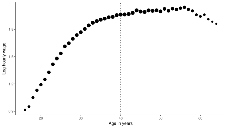
Figure 1: Average of natural logarithm of hourly wage by age of the worker. Vertical line indicates the cutoff value of 40 years for the placebo treatment. Volume of dots is proportional to share of workers in the full CPS data with the corresponding age.

For our exercise, we draw many small random samples from the full CPS data, and estimate the effect of the artificial treatment using an RDD, with log hourly wage as the outcome and age as the running variable, on each of them. Figure 1 therefore plots the true CEF of log hourly wages given age for the population from which our samples are taken. In particular, we draw random samples of size $N_{h}\in\{100,500,2000,10000\}$, from the set of individuals in the full CPS data whose age differs by no more than $h\in\{5,10,15,\infty\}$ from the placebo cutoff of 40. In each sample, we use OLS to estimate the regression

$$\begin{split}\log(\text{WAGE}_{i})&=\alpha_{h}+\tau_{h}\cdot\mathbb{I}\left\{\text{AGE}_{i}\geq 40\right\}+\sum_{j=1}^{p}\beta_{hj}^{-}\cdot(\text{AGE}_{i}-40)^{p}\\ &\qquad+\sum_{j=1}^{p}\beta_{hj}^{+}\cdot\mathbb{I}\left\{\text{AGE}_{i}\geq 40\right\}\cdot(\text{AGE}_{i}-40)^{p}+U_{i},\end{split}$$ (2.1)

for $p=1$ (a linear model with different intercept and slope on each side of the cutoff), and $p=2$ (a quadratic specification). The OLS estimate $\widehat{\tau}$ of $\tau_{h}$ is then the empirical estimate of the causal effect of the placebo treatment for workers at the threshold. The parameter $h$ is a window width (or bandwidth) that determines the range of the running variable over which the specification approximates the true CEF of log hourly wages given age. The regression coefficients in (2.1) are subscripted by $h$ because their value depends on the window width (the dependence on $p$ is left implicit). Running OLS on specification (2.1) is equivalent to local linear ($p=1$) or local quadratic ($p=2$) regression with a bandwidth $h$ and a uniform kernel function on a sample with $N_{h}$ individuals whose age differs by less than $h$ from the threshold.

Since we know the true CEF in the context of our exercise, we can compute the population values of the coefficients in the model (2.1) for the various values of $h$ and $p$ under consideration by estimating it on the full CPS data. Inspection of Figure 1 shows that the model (2.1) is misspecified to some degree for all values of $h$ and $p$ under consideration, as the dots representing the true CEF of log wages never lie exactly on a straight or quadratic line (Figures LABEL:fig_data1a and LABEL:fig_data1b in Appendix C show the resulting approximations to the CEF). As a result, the parameter $\tau_{h}$, reported in the second column of Table 1, which approximates the true jump of the CEF at the placebo cutoff, is never exactly equal to zero. The degree of misspecification varies with $h$ and $p$. In the linear case ($p=1$), it is very small for $h=5$, but increases substantially for larger values of $h$. On the other hand, the quadratic model ($p=2$) is very close to being correctly specified for all values of $h$ that we consider.

To assess the accuracy of different methods for inference, in addition to the point estimate $\widehat{\tau}$, we compute both the CRV and EHW standard error (using formulas that correspond to the default settings in STATA; see below for details) in each random sample. Because the OLS estimator $\widehat{\tau}$ is centered around $\tau_{h}$, which due to misspecification of the model (2.1) differs from the true effect of zero, we expect that the 95% EHW CI, given by $[\widehat{\tau}\pm 1.96\times\text{EHW standard error}]$, contains the zero less than 95 percent of the time. However, when $\tau_{h}$ is close to zero relative to the standard deviation of $\widehat{\tau}$ we expect this distortion to be small. Moreover, if clustering by the running variable is a suitable way to correct the distortion, the CRV standard error of $\widehat{\tau}$ should generally be larger than the EHW standard error (to account for the incorrect centering), and the CRV CI, given by $[\widehat{\tau}\pm 1.96\times\text{CRV standard error}]$, should contain the true effect of zero in roughly 95 percent of the random samples across all specifications.

2.2.  Main results

Table 1: Performance of EHW and CRV inference for placebo treatment.

				Average SE		Rate CRV SE [2pt] $>$ EHW SE	CI coverage rate
$h$	$\tau_{h}$	$N_{h}$	$SD(\widehat{\tau})$	CRV	EHW		CRV	EHW
Linear Specification ($p=1$)
5	$-0.008$	100	0.239	0.166	0.234	0.14	0.773	0.938
		500	0.104	0.073	0.104	0.13	0.780	0.947
		2000	0.052	0.036	0.052	0.13	0.773	0.949
		10000	0.021	0.015	0.023	0.09	0.772	0.961
10	$-0.023$	100	0.227	0.193	0.223	0.26	0.873	0.939
		500	0.099	0.086	0.099	0.25	0.876	0.944
		2000	0.049	0.044	0.050	0.27	0.860	0.930
		10000	0.021	0.021	0.022	0.39	0.781	0.829
15	$-0.063$	100	0.222	0.197	0.216	0.31	0.884	0.927
		500	0.095	0.089	0.096	0.34	0.853	0.899
		2000	0.048	0.047	0.048	0.45	0.712	0.730
		10000	0.020	0.028	0.021	0.92	0.348	0.153
$\infty$	$-0.140$	100	0.208	0.196	0.205	0.38	0.856	0.886
		500	0.091	0.094	0.091	0.54	0.673	0.667
		2000	0.045	0.058	0.046	0.93	0.292	0.134
		10000	0.019	0.043	0.020	1.00	0.006	0.000
Quadratic Specification ($p=2$)
5	$-0.010$	100	0.438	0.206	0.427	0.03	0.607	0.932
		500	0.189	0.086	0.190	0.01	0.599	0.947
		2000	0.093	0.042	0.095	0.01	0.587	0.951
		10000	0.038	0.018	0.042	0.00	0.595	0.964
10	$0.008$	100	0.361	0.258	0.349	0.15	0.795	0.933
		500	0.157	0.110	0.156	0.12	0.790	0.948
		2000	0.077	0.055	0.078	0.11	0.794	0.947
		10000	0.033	0.025	0.035	0.13	0.808	0.956
15	$0.014$	100	0.349	0.270	0.329	0.20	0.836	0.923
		500	0.146	0.117	0.147	0.18	0.851	0.946
		2000	0.073	0.058	0.073	0.17	0.839	0.946
		10000	0.031	0.026	0.033	0.18	0.828	0.937
$\infty$	$-0.001$	1	0.316	0.267	0.303	0.26	0.876	0.930
		500	0.134	0.117	0.135	0.24	0.890	0.949
		2000	0.068	0.058	0.067	0.23	0.887	0.947
		10000	0.029	0.027	0.030	0.26	0.910	0.960

Note: Results are based on 10,000 simulation runs.

Table 1 reports the empirical standard deviation of $\widehat{\tau}$ across simulation runs, the average values of the EHW and CRV standard errors, the proportion of runs in which the CRV standard error was larger than the EHW standard error, and the empirical coverage probabilities of the EHW and CRV CI with nominal level 95%. These results are as expected regarding the properties of EHW standard errors and CIs. They also show, however, that the CRV standard error is a downward-biased estimator of the standard deviation of $\widehat{\tau}$ in almost all the specifications that we consider, and is thus typically smaller than the EHW standard error. Correspondingly, the CRV CI has coverage properties that are mostly worse than those of the EHW CI.

A closer inspection of Table 1 reveals further interesting patterns. Consider first the quadratic specification $(p=2)$, which, as pointed out above, is close to correct for all bandwidth values. First, we see that when holding the value of $h$ constant, the coverage rate of the CRV CI is hardly affected by changes in the sample size, and always below the nominal level of 95%. The undercoverage for $h=5$ is very severe, about 35 percentage points, and decreases as the value of $h$, and thus the number of “clusters” in the data, increases. However, it still amounts to 4–6 percentage points for $h=\infty$, in which case there are, respectively, 24 and 25 “clusters” below and above the threshold. Third, the EHW CI has close to correct coverage for all bandwidth values since the degree of misspecification is small.

Next, consider the results for the linear model ($p=1$), in which the degree of misspecification increases with the bandwidth. First, we see that when holding the sample size constant the value of the CRV standard error is increasing in $h$. The CRV standard error is downward-biased for the standard deviation of $\widehat{\tau}$ when either $N_{h}$ or $h$ are small, and upward-biased if both are large (in the latter case, misspecification is substantial relative to sampling uncertainty). Second, even when the CRV standard error is larger than the EHW standard error, the corresponding CIs still undercover by large amounts.

In summary, our results suggest that if the specification (2.1) is close to correct, clustering by the running variable shrinks the estimated standard error, and thereby leads to a CI that is too narrow. This effect is particularly severe if the number of clusters is small. On the other hand, if misspecification is sufficiently severe relative to the sampling uncertainty, clustering by the running variable increases the standard error, but the resulting CIs often still remain too narrow. In the following sections, we derive theoretical results about the properties of CRV standard errors that shed further light on these findings.

Remark 1.

The results of our simulation exercise illustrate the potential severity of the issues caused by clustering standard errors at the level running variable in discrete RDDs. However, one might be concerned the results are driven by some specific feature of the CPS data. Another possible reservation is that by varying the bandwidth $h$ we vary both the degree of model misspecification and the number of “clusters”, and cluster-robust standard errors are well-known to have statistical issues in other settings with a few clusters. To address these potential concerns, we report the results of another simulation experiment in the supplemental material. In that simulation study, the data are fully computer generated, and we consider several data generating processes in which we vary the degree of misspecification and the number of support points of the running variable independently. These additional simulations confirm the qualitative results reported in this section.

Remark 2.

The clustered standard error used in our simulation exercise corresponds to the default setting in STATA. Although its formula, given in Section 3 below, involves a “few clusters” adjustment, this variance estimator is known to be biased when the number of clusters is small. One might therefore be concerned that the unsatisfactory performance of CRV CIs is driven by this issue, and that these CIs might work as envisioned by LC if one used one of the alternative variance estimators suggested in the literature on inference with few clusters. To address this concern, we repeat both the CPS placebo study and the simulation exercise described in Remark 1 using a bias-reduction modification of the STATA formula developed by Bell and McCaffrey (2002) that is analogous to the HC2 modification of the EHW standard error proposed by MacKinnon and White (1985). The results are reported in the supplemental material. The main findings are as follows. When combined with an additional critical value adjustment, also due to Bell and McCaffrey (2002), this fixes the undercoverage of CRV CIs in settings where the specification (2.1) is close to correct. However, this comes at a substantial loss in power relative to EHW CIs, which also have approximately correct coverage in this case (the CIs are more than twice as long in some specifications than EHW CIs). Under more severe misspecification, the adjustments tend to improve coverage relative to EHW CIs somewhat, but both types of CIs generally still perform poorly. Using bias-corrected standard errors does therefore not make CRV CIs robust to misspecification of the CEF.

3.  Econometric Framework

In this section, we first review the sharp RDD, and formally define the treatment effect estimator and the corresponding standard errors and CIs. We then discuss LC’s motivation for clustering the standard errors by the running variable, and point out some conceptual shortcomings.

3.1.  Model, Estimator and CIs

In a sharp RDD, we observe a random sample of $N$ units from some large population. Let $Y_{i}(1)$ and $Y_{i}(0)$ denote the potential outcome for the $i$th unit with and without receiving treatment, respectively, and let $T_{i}\in\{0,1\}$ be an indicator variable for the event that the unit receives treatment. The observed outcome is given by $Y_{i}=(1-T_{i})Y_{i}(0)+T_{i}Y_{i}(1)$. A unit is treated if and only if a running variable $X_{i}$ crosses a known threshold, which we normalize to zero, so that $T_{i}=\mathbb{I}\left\{X_{i}\geq 0\right\}$. Let $\mu(X_{i})=\mathbb{E}[Y_{i}\mid X_{i}]$ denote the conditional expectation of the observed outcome given the running variable. If the CEFs for the potential outcomes $\mathbb{E}[Y_{i}(1)\mid X_{i}]$ and $\mathbb{E}[Y_{i}(0)\mid X_{i}]$ are continuous at the threshold, then the discontinuity in $\mu(x)$ at zero is equal to the average treatment effect (ATE) for units at the threshold,

$$\tau=\mathbb{E}(Y_{i}(1)-Y_{i}(0)\mid X_{i}=0)=\lim_{x\downarrow 0}\mu(x)-\lim_{x\uparrow 0}\mu(x).$$

A standard approach to estimate $\tau$ is to use local polynomial regression. In its simplest form, this estimation strategy involves fixing a window width, or a bandwidth, $h>0$, and a polynomial order $p\geq 0$, with $p=1$ and $p=2$ being the most common choices in practice. One then discards all observations for which the running variable is outside the estimation window $[-h,h]$, keeping only the $N_{h}$ observations $\{Y_{i},X_{i}\}_{i=1}^{N_{h}}$ for which $\lvert X_{i}\rvert\leq h$, and runs an OLS regression of the outcome $Y_{i}$ on a vector of covariates $M_{i}$ consisting of an intercept, polynomial terms in the running variable, and their interactions with the treatment indicator. The ATE estimator $\widehat{\tau}$ of $\tau$ is then given by the resulting OLS estimate on the treatment indicator. Without loss of generality, we order the components of $M_{i}$ such that this treatment indicator is the first one, so

$$\widehat{\tau} =e_{1}^{\prime}\widehat{\theta},\qquad\widehat{\theta}=\widehat{Q}^{-1}\frac{1}{N_{h}}\sum_{i=1}^{N_{h}}M_{i}Y_{i},\qquad\widehat{Q}=\frac{1}{N_{h}}\sum_{i=1}^{N_{h}}M_{i}M_{i}^{\prime},\qquad M_{i}=m(X_{i}),$$

$$m(x) =(\mathbb{I}\left\{x\geq 0\right\},\mathbb{I}\left\{x\geq 0\right\}x,\ldots,\mathbb{I}\left\{x\geq 0\right\}x^{p},1,x,\ldots,x^{p})^{\prime},$$

where $e_{1}=(1,0,\ldots,0)^{\prime}$ denotes the first unit vector. When $p=1$, for instance, $\widehat{\tau}$ is simply the difference between the intercepts from separate linear regressions of $Y_{i}$ on $X_{i}$ to the left and to the right of the threshold. The conventional Eicker-Huber-White (EHW) or heteroskedasticity-robust standard error of $\widehat{\tau}$ is $\widehat{\sigma}_{\textnormal{EHW}}/\sqrt{N_{h}}$, where $\widehat{\sigma}_{\textnormal{EHW}}^{2}$ is the top-left element of the EHW estimator of the asymptotic variance of $\widehat{\theta}$. That is,

$$\widehat{\sigma}_{\textnormal{EHW}}^{2} =e_{1}^{\prime}\widehat{Q}^{-1}\widehat{\Omega}_{\textnormal{EHW}}\widehat{Q}^{-1}e_{1}, \widehat{\Omega}_{\textnormal{EHW}} =\frac{1}{N_{h}}\sum_{i=1}^{N_{h}}\widehat{u}_{i}^{2}M_{i}M_{i}^{\prime}, \widehat{u}_{i} =Y_{i}-M_{i}^{\prime}\widehat{\theta}.$$

An alternative standard error, proposed by LC for RDDs with a discrete running variable, is $\widehat{\sigma}_{\textnormal{CRV}}/\sqrt{N_{h}}$. Here $\widehat{\sigma}_{\textnormal{CRV}}^{2}$ is the top-left element of the “cluster-robust” estimator of the asymptotic variance of $\widehat{\theta}$ that clusters by the running variable (CRV). That is, the estimator treats units with the same realization of the running variable as belonging to the same cluster (Liang and Zeger, 1986). Denoting the $G_{h}$ support points inside the estimation window by $\{x_{1},\dotsc,x_{G_{h}}\}$, the estimator $\widehat{\sigma}_{\textnormal{CRV}}^{2}$ has the form

$$\widehat{\sigma}_{\textnormal{CRV}}^{2}=e_{1}^{\prime}\widehat{Q}^{-1}\widehat{\Omega}_{\textnormal{CRV}}\widehat{Q}^{-1}e_{1},\quad\widehat{\Omega}_{\textnormal{CRV}}=\frac{1}{N_{h}}\sum_{g=1}^{G_{h}}\sum_{i=1}^{N_{h}}\mathbb{I}\left\{X_{i}=x_{g}\right\}\widehat{u}_{i}M_{i}\sum_{j=1}^{N_{h}}\mathbb{I}\left\{X_{j}=x_{g}\right\}\widehat{u}_{j}M_{j}^{\prime}.$$

The EHW and CRV CIs for $\tau$ with nominal level $1-\alpha$ based on these standard errors are then given by

$$\widehat{\tau}\pm z_{1-\alpha/2}\times\widehat{\sigma}_{\textnormal{EHW}}/\sqrt{N_{h}},\quad\textrm{ and }\quad\widehat{\tau}\pm z_{1-\alpha/2}\times\widehat{\sigma}_{\textnormal{CRV}}/\sqrt{N_{h}},$$

respectively, where the critical value $z_{1-\alpha/2}$ is the $1-\alpha/2$ quantile of the standard normal distribution. In particular, for a CI with 95% nominal coverage we use $z_{0.975}\approx 1.96$.

3.2.  Potential issues due to discreteness of the running variable

Whether the EHW CI is valid for inference on $\tau$ largely depends on the bias properties of the ATE estimator $\widehat{\tau}$. It follows from basic regression theory that in finite samples, $\widehat{\tau}$ is approximately unbiased for its population counterpart $\tau_{h}$, given by

$$\tau_{h} =e_{1}^{\prime}\theta_{h}, \theta_{h} =Q^{-1}\mathbb{E}[M_{i}Y_{i}\mid\lvert X_{i}\rvert\leq h], Q =\mathbb{E}[M_{i}M_{i}^{\prime}\mid\lvert X_{i}\rvert\leq h]$$

(for simplicity, we leave the dependence of $\tau_{h}$ on $p$ implicit). However, $\widehat{\tau}$ is generally a biased estimator of $\tau$. The magnitude of the bias, $\tau_{h}-\tau$, is determined by how well $\mu(x)$ is approximated by a $p$th order polynomial within the estimation window $[-h,h]$. If $\mu(x)$ was a $p$th order polynomial function, then $\tau_{h}=\tau$, but imposing this assumption is typically too restrictive in applications.

The EHW CI is generally valid for inference on $\tau_{h}$ since, if $p$ is fixed, the $t$-statistic based on the EHW standard error has a standard normal distribution in large samples. That is, as $N_{h}\to\infty$, under mild regularity conditions,

$$\sqrt{N_{h}}(\widehat{\tau}-\tau_{h})/\widehat{\sigma}_{\textnormal{EHW}}\stackrel{{\scriptstyle d}}{{\rightarrow}}\mathcal{N}(0,1).$$ (3.1)

Using the EHW CI for inference on $\tau$ is therefore formally justified if the bias $\tau_{h}-\tau$ is asymptotically negligible relative to the standard error, in these sense that their ratio converges in probability to zero,

$$\frac{\tau_{h}-\tau}{\widehat{\sigma}_{\textnormal{EHW}}/\sqrt{N_{h}}}\stackrel{{\scriptstyle P}}{{\rightarrow}}0.$$ (3.2)

Choosing a window width $h$ such that condition (3.2) is satisfied is called “undersmoothing” in the nonparametric regression literature. If the distribution of the running variable $X_{i}$ is continuous, then (3.2) holds under regularity conditions provided that $h\to 0$ sufficiently quickly as the sample size grows, and that $\mu(x)$ is sufficiently smooth (e.g. Hahn et al., 2001, Theorem 4). This result justifies the use of the EHW standard errors for inference on $\tau$ when $X_{i}$ has rich support and $h$ is chosen sufficiently small.

In principle, the EHW CI is also valid for inference on $\tau$ when the distribution of $X_{i}$ is discrete, as long as there is some justification for treating the bias $\tau_{h}-\tau$ as negligible in the sense of condition (3.2). This justification becomes problematic, however, if the gaps between the support points closest to the threshold are sufficiently wide. This is because, to ensure that $N_{h}$ is large enough to control the sampling variability of $\widehat{\tau}$ and to ensure that the normality approximation (3.1) is accurate, a researcher may be forced to choose a window width $h$ that is “too large”, in the sense that the bias-standard error ratio is likely to be large. When the running variable is discrete, the EHW CI might therefore not be appropriately centered, and thus undercover in finite samples.

3.3.  Motivation for clustering by the running variable

To address the problems associated EHW standard errors discussed above, LC proposed using CRV standard errors when the running variable is discrete. This approach has since found widespread use in empirical economics. The rationale provided by LC is as follows. Let $\delta(x)=\mu(x)-m(x)^{\prime}\theta_{h}$ denote the specification bias of the (local) polynomial approximation to the true CEF, and write $\delta_{i}=\delta(X_{i})$. Then, for observations inside the estimation window, we can write

$$Y_{i}=M_{i}^{\prime}\theta_{h}+u_{i},\qquad u_{i}=\delta_{i}+\varepsilon_{i},$$ (3.3)

where $\varepsilon_{i}=Y_{i}-\mu(X_{i})$ is the deviation of the observed outcome from its conditional expectation, and the value of $\delta_{i}$ is identical for all units that share the same realization of the running variable. LC then treat $\delta_{i}$ as a random effect, rather than a specification error that is non-random conditional on the running variable. That is, they consider a model that has the same form as (3.3), but where $\delta_{i}=\sum_{g=1}^{G_{h}}D_{g}\mathbb{I}\left\{X_{i}=x_{g}\right\}$, with $D=(D_{1},\dotsc,D_{G_{h}})$ a mean-zero random vector with elements that are mutually independent and independent of $\{(X_{i},\varepsilon_{i})\}_{i=1}^{N_{h}}$. Under this assumption, equation (3.3) is a correctly specified regression model in which the error term $u_{i}$ exhibits within-group correlation at the level of the running variable. That is, for $i\neq j$, we have that $\mathbb{E}(u_{i}u_{j}|X_{i}=X_{j})\neq 0$ and $\mathbb{E}(u_{i}u_{j}|X_{i}\neq X_{j})=0$. LC then argue that due to this group structure, the variance estimator $\widehat{\sigma}_{\textnormal{CRV}}^{2}$ is appropriate.

This rationale is unusual in several respects. First, it is not compatible with the standard assumption that the data are generated by i.i.d. sampling from a fixed population, with a non-random CEF. Under i.i.d. sampling, $\delta_{i}=\delta(X_{i})$ is not random conditional on $X_{i}$, as the function $\delta(x)$ depends only on the population distribution of observable quantities, and does not change across repeated samples. Assuming that $\delta(x)$ is random implies that the CEF $\mu(x)=m(x)^{\prime}\theta_{h}+\delta(x)$ changes across repeated samples, since in each sample one observes a different realization of $D$, and thus different deviations $\delta(x)$ of the CEF from its “average value” $m(x)^{\prime}\theta_{h}$.

Second, the randomness of the CEF in the LC model implies that the ATE $\tau$, which is a function of the CEF, is also random. This makes it unclear what the population object is that the RDD identifies, and the CRV CIs provide inference for. One might try to resolve this problem by defining the parameter of interest to be $\tau_{h}$, the magnitude of the discontinuity of the “average” CEF $\mathbb{E}(Y_{i}\mid X_{i})=\mathbb{E}(\mathbb{E}(Y_{i}\mid X_{i},D\mid X_{i}))=M_{i}^{\prime}\theta_{h}$, where the average is taken over the specification errors. But it is unclear in what sense $\tau_{h}$ measures a causal effect, as it does not correspond to an ATE for any particular set of units. Furthermore, proceeding like this amounts to assuming that the chosen polynomial specification is correct after all, which seems to contradict the original purpose of clustering by running variable. Alternatively, one could consider inference on the conditional expectation of the (random) ATE given specification errors, $\mathbb{E}(\tau\mid D)$. But once we condition on $D$, the data are i.i.d., the LC model becomes equivalent to the standard setup described in Section 3.1, and all the concerns outlined in Section 3.2 apply.

Third, the LC model effectively rules out smooth CEFs. To see this, note that if the CEF $\mu(x)$ were smooth, then units with similar values of the running variable should also have a similar value of the specification error $\delta(X_{i})$. In the LC model, the random specification errors are independent for any two values of the running variable, even if the values are very similar. Since in most empirical applications, one expects a smooth relationship between the outcome and the running variable, this is an important downside.

Due to these issues, we argue that the LC model should not be viewed as a literal description of the DGP, but rather as a heuristic device to motivate using CRV standard errors. Their performance should be evaluated under the standard framework outlined in Section 3.1, in which the data are generated by i.i.d. sampling from a fixed population distribution.

4.  Theoretical properties of CRV confidence intervals

In this section, we study the properties of $\widehat{\sigma}_{\textnormal{CRV}}^{2}$ under the standard setup introduced in Section 3.1, which then directly leads to statements about the coverage properties of the corresponding CIs. The results reported here summarize the main insights from a more formal analysis in Appendix A. To capture the notion that $\mu(x)$ is “close” to a polynomial specification, our asymptotic analysis uses a sequence of data generating processes (DGPs) under which the CEF $\mu(x)$ changes with the sample size, so that it lies within an $N_{h}^{-1/2}$ neighborhood of the polynomial specification $m(x)^{\prime}\theta_{h}$ uniformly over the estimation window $[-h,h]$. Changing the DGP with the sample size is a widely used technical device that helps preserve important finite-sample issues in the asymptotic approximation. In our setting, it allows us capture the fact that it may be unclear in finite samples whether the chosen polynomial specification is correct.

This setup implies that there are constants $b$ and $d_{1},\ldots,d_{G_{h}}$ such that, as the sample size increases,

$$\sqrt{N_{h}}(\tau_{h}-\tau)\to b\quad\textrm{ and }\quad\sqrt{N_{h}}\delta(x_{g})\to d_{g}$$

for each support point $x_{g}$ in the estimation window. Lemma 1 in Appendix A then shows that in large samples, $\sqrt{N}_{h}(\widehat{\tau}-\tau_{h})$ is normally distributed with mean zero and asymptotic variance

$$\sigma^{2}_{\tau}=\sum_{g=1}^{G_{h}}\sigma^{2}_{g}\omega_{g},\qquad\omega_{g}=e_{1}^{\prime}Q^{-1}Q_{g}Q^{-1}e_{1},$$

where $\sigma^{2}_{g}=\mathbb{V}(Y_{i}\mid X_{i}=x_{g})$ denotes the conditional variance of the outcome given the running variable, $Q_{g}=\pi_{g}m(x_{g})m(x_{g})^{\prime}$ and $\pi_{g}=P(X_{i}=x_{g}\mid\lvert X_{i}\rvert\leq h)$ is the probability that the value of the running variable for a unit within the estimation window equals $x_{g}$, the $g$th support point. The asymptotic variance $\sigma^{2}_{\tau}$ is a weighted sum of the conditional variances of the outcome given the running variable, with the weights $\omega_{g}$ reflecting the influence of observations with $X_{i}=x_{g}$ on the estimate $\widehat{\tau}$. It follows that in large samples, $\sqrt{N}_{h}(\widehat{\tau}-\tau)$ is normally distributed with asymptotic bias $b$ and variance $\sigma^{2}_{\tau}$. Lemma 1 also shows that the EHW variance estimator is consistent for $\sigma^{2}_{\tau}$.

As discussed in Section 3.1, CIs based on EHW standard errors generally undercover $\tau$, as they are not correctly centered unless $b=0$. A CI based on the CRV standard error $\widehat{\sigma}_{\textnormal{CRV}}/\sqrt{N_{h}}$ is centered at the same point estimate. In order for a CRV CI to have correct coverage, the CRV standard error thus has to be larger than the EHW standard error by a suitable amount, at least on average. In the remainder of this section, we show that this is not the case, and that CIs based on CRV standard errors (i) undercover the ATE under correct specification and (ii) can either over- or undercover the ATE under misspecification by essentially arbitrary amounts. The asymptotic behavior of $\widehat{\sigma}_{\textnormal{CRV}}^{2}$ differs depending on whether the number of support points inside the estimation window ${G}_{h}$ is treated as fixed or as increasing with the sample size. We examine each of these two cases in turn now.

4.1.  Fixed number of support points

In Theorem 1 in Appendix A, we study the properties of $\widehat{\sigma}_{\textnormal{CRV}}^{2}$ when ${G}_{h}$ is held fixed as the sample size increases. This should deliver useful approximations for settings with a small to moderate number of support points within the estimation window $[-h,h]$. We show that in this case $\widehat{\sigma}_{\textnormal{CRV}}^{2}$ does not converge to a constant, but to a non-degenerate limit denoted by $\widehat{\sigma}_{\textnormal{CRV},\infty}^{2}$. This means that it remains stochastic even in large samples. It follows from Theorem 1 that we can decompose the expected difference between $\widehat{\sigma}_{\textnormal{CRV},\infty}^{2}$ and $\sigma_{\tau}^{2}$ as

$$\mathbb{E}(\widehat{\sigma}_{\textnormal{CRV},\infty}^{2})-\sigma_{\tau}^{2}=\sum_{g=1}^{G_{h}}d_{g}^{2}\pi_{g}\omega_{g}+\sum_{g=1}^{G_{h}}m(x_{g})^{\prime}Q^{-1}\left(\sum_{j=1}^{G_{h}}\sigma^{2}_{j}Q_{j}-2\sigma^{2}_{g}Q\right)Q^{-1}m(x_{g})\cdot\pi_{g}\omega_{g}.$$ (4.1)

The first term on the right-hand side of (4.1) is positive, and its magnitude depends on the degree of misspecification. The second term does not depend on the degree of misspecification and vanishes if we replace the estimated regression residuals $\widehat{u}_{i}$ in the CRV formula with the true error $u_{i}$. Its sign is difficult to determine in general. It is therefore helpful to consider the case in which the conditional variance of the outcomes is homoskedastic, $\sigma^{2}_{g}=\sigma^{2}$, so that $\sigma^{2}_{\tau}=\sigma^{2}\sum_{g=1}^{G_{h}}\omega_{g}$. The expected difference between $\widehat{\sigma}_{\textnormal{CRV},\infty}^{2}$ and $\sigma_{\tau}^{2}$, relative to $\sigma^{2}_{\tau}$, can then be written as,

$$\frac{\mathbb{E}(\widehat{\sigma}_{\textnormal{CRV},\infty}^{2})-\sigma_{\tau}^{2}}{\sigma^{2}_{\tau}}=\frac{\sum_{g=1}^{G_{h}}d_{g}^{2}\pi_{g}\omega_{g}}{\sigma^{2}\sum_{g=1}^{G_{h}}\omega_{g}}-\frac{\sum_{g=1}^{G_{h}}m(x_{g})^{\prime}Q^{-1}m(x_{g})\pi_{g}\omega_{g}}{\sum_{g=1}^{G_{h}}\omega_{g}}\equiv T_{1}+T_{2}.$$ (4.2)

This decomposition is key to understanding the properties of $\widehat{\sigma}_{\textnormal{CRV}}^{2}$ in settings with a few support points $G_{h}$. Since the EHW variance estimator is consistent for $\sigma^{2}_{\tau}$, the notation introduced in (4.2) implies that average magnitude of $\widehat{\sigma}_{\textnormal{CRV}}^{2}$ is about $(1+T_{1}+T_{2})$ times that of $\widehat{\sigma}^{2}_{\textnormal{EHW}}$. In order for the CRV CI to have correct coverage, the terms $T_{1}+T_{2}$ have to be positive, with a magnitude that suitably reflects the degree of misspecification. That is generally not the case.

First, the term $T_{1}$ is indeed positive and increasing in the “average” misspecification, as measured by the average squared local specification error, $d_{g}^{2}$, weighted by the cluster size $\pi_{g}$ and $\omega_{g}$. Heuristically, this term arises because the CRV variance estimator treats the specification errors as random effects, and tries to account for their “variance”. The magnitude of $T_{1}$ depends on the magnitude of the average misspecification, relative to $\sigma^{2}$. Second, the term $T_{2}$ is negative under homoskedasticity because both the weights $\omega_{g}$ and $m(x_{g})^{\prime}Q^{-1}m(x_{g})$ are positive. We thus also expect the term to be negative for small and moderate levels of heteroskedasticity. Third, the magnitude of $T_{2}$ depends only on the marginal distribution of the running variable, and not on $\sigma^{2}$. It is therefore the dominant term in the decomposition (4.2) if the variance $\sigma^{2}$ of the error terms is large. Fourth, the term $T_{2}$ is increasing in the polynomial order $p$. To see this, observe that $\sum_{g=1}^{G_{h}}m(x_{g})^{\prime}Q^{-1}m(x_{g})\pi_{g}=\operatorname{trace}(\sum_{g=1}^{G_{h}}Q_{g}Q^{-1})=2(p+1)$. The term $T_{2}$ can thus be written as a weighted average of terms whose unweighted average is equal to $2(p+1)$. Heuristically, this means that the expected difference between $\widehat{\sigma}_{\textnormal{CRV},\infty}^{2}$ and $\sigma_{\tau}^{2}$ should be increasing with the order of the polynomial. For example, it is generally larger for local quadratic regression ($p=2$) than for local linear regression ($p=1$). Fifth, the term $T_{2}$ is analogous to the downward bias of cluster-robust variance estimators in settings with a few clusters (e.g. Cameron and Miller, 2014). While the existence of such biases is well-known in principle, in the current setting the distortion can be substantial even for moderate values of $G_{h}$, as shown by our simulations in Section 2 and the supplemental material.

In summary, our theoretical results show if the degree of misspecification relative to the variance of the residuals and the number of clusters are both small to moderate, the CRV standard error is on average smaller than the EHW standard error. Clustering the standard error by the running variable will then amplify, rather than solve, the problems for inference caused by specification bias. This problem is particularly severe under correct specification. These results are exactly in line with the evidence presented in Section 2.

4.2.  Increasing number of support points

In Theorem 2 in Appendix A, we study the properties of $\widehat{\sigma}_{\textnormal{CRV}}^{2}$ when ${G}_{h}$ increases with the sample size. This should deliver a useful approximation when there are many support points within the estimation window $[-h,h]$. We show that if $G_{h}\to\infty$ as $N_{h}\to\infty$, the variance of $\widehat{\sigma}_{\textnormal{CRV}}^{2}$ vanishes, and we obtain that

$$\widehat{\sigma}_{\textnormal{CRV}}^{2}-\sigma^{2}_{\tau}=\sum_{g=1}^{G_{h}}d_{g}^{2}\pi_{g}\omega_{g}+o_{P}(1).$$

The right-hand side coincides with the first term in Equation (4.1); the second term vanishes. This means that if the number of support points $G_{h}$ is large, the CRV standard error indeed tends to be larger than the EHW standard error, so that clustering by the running variable improves coverage of the corresponding CI.

This fact alone does not imply that CRV confidence intervals have correct coverage for all possible CEFs $\mu(\cdot)$, but only that there exist a set $\mathcal{M}_{\textnormal{CRV}}$ of CEFs over the estimation window $[-h,h]$ for which correct asymptotic coverage is delivered. While $\mathcal{M}_{\textnormal{CRV}}$ is strictly larger than the set of all $p$th order polynomial functions, this property by itself is not a sufficient argument for justifying the use of CRV CIs. This is because any inference method that leads to CIs wider than those based on EHW standard errors—including undesirable approaches such as simply adding an arbitrary constant to the EHW standard errors—gives an improvement in coverage, and delivers correct inference if the true CEF lies in some set that is strictly larger than the set of all $p$th order polynomial functions.

Whether CRV standard errors provide a meaningful degree of robustness to misspecification depends on whether $\mathcal{M}_{\textnormal{CRV}}$ contains CEFs that are empirically relevant and easy to interpret, so that it is clear in practice what types of restrictions on $\mu(x)$ the researcher is imposing. In this respect, the set $\mathcal{M}_{\textnormal{CRV}}$ has the undesirable feature that it depends on the distribution of the running variable through the weights $\omega_{g}$ and the relative cluster sizes $\pi_{g}$. This makes the set difficult to characterize. Furthermore, it implies that two researchers studying the same RDD may arrive to different conclusions if, say, one of them oversampled observations closer to the cutoff (so that the relative cluster size $\pi_{g}$ for those observations is larger). Finally, simulation results in the supplemental material show that the set does not include mild departures from a polynomial specification, which is in line with the intuition given in Section 3.3 that the model that motivates the CRV approach implicitly rules out smooth CEFs.

For these reasons, when the number of support points within the estimation window is large, and the researcher is worried that $\widehat{\tau}$ is biased, a better alternative to using CRV CIs is to choose a smaller bandwidth. Alternatively, one can use one of the honest inference procedures that we outline in Section 5, which guarantee proper coverage under easily interpretable restrictions on $\mu(x)$.

5.  Honest Confidence Intervals

If the CEF $\mu(x)$ is allowed to vary arbitrarily between the two support points of the running variable closest to the threshold, no method for inference on the ATE can be both valid and informative: without any restrictions on $\mu(x)$, even in large samples, any point on the real line would remain a feasible candidate for the value of $\tau$. To make progress, we need to place constraints on $\mu(x)$. Formally, we impose the assumption that $\mu\in\mathcal{M}$ for some class of functions $\mathcal{M}$, and then seek to construct CIs $C^{1-\alpha}$ that satisfy

$$\liminf_{N\to\infty}\inf_{\mu\in\mathcal{M}}P_{\mu}(\tau\in C^{1-\alpha})\geq 1-\alpha,$$ (5.1)

where the notation $P_{\mu}$ makes explicit that the coverage probability depends on the CEF. Following the terminology in Li (1989), we refer to such CIs as honest with respect to $\mathcal{M}$. Honesty with respect to a meaningful and interpretable function class is desirable for a CI, as it guarantees good coverage properties even when facing the “the worst possible” CEF that still satisfies the postulated constraints. In the following subsections, we present honest CIs with respect to two different function classes, which correspond to two different formalizations of the notion that $\mu(x)$ can be well-approximated by a polynomial. The implementation of these CIs is straightforward using the software package RDHonest, available at https://github.com/kolesarm/RDHonest. Proofs are relegated to Appendix B.

5.1.  Bound on the second derivative

The first restriction on $\mu(x)$ that we consider is based on bounding the magnitude of its second derivative, which is perhaps the most natural way of imposing smoothness. Specifically, we assume that $\mu(x)$ is twice differentiable on either side of the cutoff, with a second derivative that is bounded in absolute value by a known constant $K$. By choosing a value of $K$ close to zero, the researcher can thus formalize the notion that $\mu(x)$ is close to being linear, whereas choosing a large value of $K$ allows for less smooth CEFs. For technical reasons we only require $\mu(x)$ to be twice differentiable almost everywhere, which leads to the second-order Hölder class

$$\mathcal{M}_{\textnormal{H}}(K)=\{\mu\colon\lvert\mu^{\prime}(a)-\mu^{\prime}(b)\rvert\leq K\lvert a-b\rvert\textrm{ for all }a,b\in\mathbb{R}_{-}\textrm{ and all }a,b\in\mathbb{R}_{+}\}.$$

A local version of this assumption is used in Cheng et al. (1997), whose results formally justify using local polynomial regression to estimate the ATE parameter when the running variable is continuous. Our goal is inference: we seek to construct CIs that are honest with respect to $\mathcal{M}_{\textnormal{H}}(K)$, and based on a local linear estimator $\widehat{\tau}$ as defined in Section 3 (with $p=1$). This can be accomplished using results in Armstrong and Kolesár (2016), who study the construction of honest CIs in general nonparametric regression problems.

It turns out that it is easier to construct CIs that are honest conditional on the realizations of the running variable, which is a slightly stronger condition than (5.1). To explain the construction, let $\widetilde{\tau}_{h}=\mathbb{E}(\widehat{\tau}\mid X_{1},\dotsc,X_{N_{h}})$ denote conditional expectation of the treatment effect estimator, and let $\widehat{\sigma}^{2}_{\textnormal{NN}}/N_{h}$ denote the nearest-neighbor estimator (Abadie and Imbens, 2006; Abadie et al., 2014) of $\mathbb{V}(\widehat{\tau}\mid X_{1},\dotsc,X_{N_{h}})$, the conditional variance of $\widehat{\tau}$. With discrete running variable, this estimator can be written as

$$\widehat{\sigma}^{2}_{\textnormal{NN}}=e_{1}^{\prime}\widehat{Q}^{-1}\widehat{\Omega}_{\textnormal{NN}}\widehat{Q}^{-1}e_{1},\qquad\widehat{\Omega}_{\textnormal{NN}}=\frac{1}{N_{h}}\sum_{g=1}^{G_{h}}n_{g}\widehat{\sigma}^{2}_{g}m(x_{g})m(x_{g})^{\prime},$$

where $n_{g}$ is the number of observations with $X_{i}=x_{g}$, and $\widehat{\sigma}^{2}_{g}=\sum_{i\colon X_{i}=x_{g}}(Y_{i}-\overline{Y}_{g})^{2}/(n_{g}-1)$ is an unbiased estimator of the conditional variance $\sigma^{2}_{g}=\mathbb{V}(Y_{i}\mid X_{i}=x_{g})$, with $\overline{Y}_{g}=n_{g}^{-1}\sum_{i\colon X_{i}=x_{g}}Y_{i}$. We can decompose the $t$-statistic based on this variance estimator as

$$\frac{\widehat{\tau}-\tau}{\widehat{\sigma}_{\textnormal{NN}}/\sqrt{N_{h}}}=\frac{\widehat{\tau}-\widetilde{\tau}_{h}}{\widehat{\sigma}_{\textnormal{NN}}/\sqrt{N_{h}}}+\frac{\widetilde{\tau}_{h}-\tau}{\widehat{\sigma}_{\textnormal{NN}}/\sqrt{N_{h}}}.$$

Under mild regularity conditions, a Central Limit Theorem ensures that the first term has standard normal distribution in large samples, and the second term is bounded in absolute value by

$$r_{\sup}=\frac{\sup_{\mu\in\mathcal{M}_{H}(K)}\lvert\widetilde{\tau}_{h}-\tau\rvert}{\widehat{\sigma}_{\textnormal{NN}}/\sqrt{N_{h}}}.$$

In Appendix B, we show that the supremum on the right-hand side of the last equation is attained by the function $\mu(x)$ that equals $-Kx^{2}$ for $x\geq 0$ and $Kx^{2}$ for $x<0$. This yields the explicit expression

$$r_{\sup} =-\frac{K}{2}\frac{\sum_{i=1}^{N_{h}}w(X_{i})X_{i}^{2}\operatorname{sign}(X_{i})}{\widehat{\sigma}_{\textnormal{NN}}/\sqrt{N_{h}}}, w(X_{i}) =\frac{1}{N_{h}}\cdot e_{1}^{\prime}\widehat{Q}^{-1}M_{i},$$ (5.2)

for the upper bound $r_{\sup}$ on the second component of the $t$-statistic. This approach of bounding the second derivative (BSD) thus leads to the following CI:

Proposition 1.

Let $\operatorname{cv}_{1-\alpha}(r)$ denote the $1-\alpha$ quantile of the $\lvert\mathcal{N}(r,1)\rvert$ distribution (the distribution of the absolute value of a normal random variable with mean $r$ and variance 1). Then, under regularity conditions stated in Appendix B, the CI

$$C_{\textnormal{BSD}}^{1-\alpha}=\left(\widehat{\tau}\pm\operatorname{cv}_{1-\alpha}(r_{\sup})\times\widehat{\sigma}_{\textnormal{NN}}/\sqrt{N_{h}}\right).$$ (5.3)

is honest with respect to $\mathcal{M}_{\textnormal{H}}(K)$.

This CI has several attractive features. First, since the CI is valid conditional on the realizations of the running variable, it is not necessary to distinguish between the cases of a discrete and a continuous distribution of the running variable. The CI is valid in both cases. Second, $C_{\textnormal{BSD}}^{1-\alpha}$ takes into account the exact finite-sample bias of the estimator, and is thus valid for any choice of bandwidth. In particular, it does not rely on asymptotic promises about what the bandwidth would have been had the sample size been larger, and remains valid even if the bandwidth is treated as fixed. In contrast, the usual methods of inference in RDDs rely on the assumption that the bandwidth shrinks to zero sufficiently quickly relative to the sample size, which can be hard to evaluate in practice. Third, to achieve the tightest possible CI, one can simply choose a bandwidth $h$ that minimizes its length $2\operatorname{cv}_{1-\alpha}(r_{\sup})\times\widehat{\sigma}_{\textnormal{NN}}/\sqrt{N_{h}}$. Since this quantity depends on the outcome data only through the variance estimate $\widehat{\sigma}_{\textnormal{NN}}$, which does not depend on $\mu$, and which can be shown to be consistent under mild regularity conditions, doing so does not invalidate the honesty of the resulting CI.

An important implementation aspect of $C_{\textnormal{BSD}}^{1-\alpha}$ is that it requires the researcher to choose a value for $K$. This choice reflects the researcher’s beliefs of what constitutes a plausible level of fluctuation in the function $\mu(x)$ in the particular empirical context. In practice, we recommend reporting results for a range of $K$ values in order to illustrate the sensitivity of empirical conclusions to this choice. We find the following heuristic useful to get an intuition for the restrictions implied by particular choices of $K$. Consider the function $\mu$ over some interval $[x^{*},x^{**}]$. One can show by simple algebra that if $\mu\in\mathcal{M}_{\textnormal{H}}(K)$, then it differs by at most $K\times(x^{**}-x^{*})^{2}/8$ from a straight line between $\mu(x^{*})$ and $\mu(x^{**})$. Thus, if a researcher believes, for example, that the CEF differs by no more than $S$ from a straight line between the CEF values at the endpoints of any interval of length one in the support of the running variable, a reasonable choice for the bound on the second derivative is $K=8S$.

The use of subject knowledge for choosing $K$ is necessary, as it is not possible to use a data-driven method without additional assumptions. In particular, it follows from the results in Low (1997) and Armstrong and Kolesár (2017) that it is not possible to form honest CIs that are tighter than those in Proposition 1 by using data-dependent tuning parameters, and at the same time maintain coverage over the whole function class $\mathcal{M}_{\textnormal{H}}(K)$, for some conservative upper bound $K$. This is related to the fact that it is not possible to upper bound $K$ from the data. It is possible, however, to lower bound $K$ from the data. In the supplemental material, we construct an estimate and a left-sided CI for this lower bound by adapting the construction from Armstrong and Kolesár (2017) to our setup. We apply this method to the two empirical applications in Section 6 below. The left-sided CI can be used as a specification test to check if the chosen value of $K$ is too low to be compatible with the data.

5.2.  Bounds on specification errors at the threshold

The second restriction on $\mu(x)$ that we consider formalizes the intuitive notion that the chosen model fits no worse at the cutoff than anywhere else in the support of the running variable within the estimation window $[-h,h]$. In particular, we assume that the left limit of the specification bias at the threshold, $\lim_{x\uparrow 0}\delta(x)$, is no larger than the specification bias $\delta(x_{g})$ at any point $x_{g}$ in the support of the running variable below the threshold, and similarly for the right limit. This leads to the class

$$\mathcal{M}_{\textnormal{BME}}(h)=\left\{\mu\colon|\lim_{x\uparrow 0}\delta(x)|\leq\max_{1\leq g\leq G_{h}^{-}}|\delta(x_{g})|\textnormal{ and }|\lim_{x\downarrow 0}\delta(x)|\leq\max_{G_{h}^{-}<g\leq G_{h}}|\delta(x_{g})|\right\},$$

where we assume that the support points $\{x_{1},\dotsc,x_{G_{h}}\}$ are ordered so that the first $G_{h}^{-}$ points are below the cutoff, and $\delta(x)\equiv\mu(x)-m(x)^{\prime}\theta_{h}$ is the specification bias. Note that the specification bias depends on the function $\mu(x)$ directly, but also indirectly as the definition of the best polynomial predictor $m(x)^{\prime}\theta_{h}$ depends on $\mu(x)$. We refer to this class as the bounded misspecification error (BME) class.

The assumption that $\mathcal{M}_{\textnormal{BME}}(h)$ contains the true CEF implies that we can bound the bias $\tau_{h}-\tau$ as follows:

$$|\tau_{h}-\tau|\leq b_{\max},\qquad b_{\max}\equiv\max_{G_{h}^{-}<g\leq G_{h}}|\delta(x_{g})|+\max_{1\leq g\leq G_{h}^{-}}|\delta(x_{g})|.$$

It will be convenient to rewrite the bias bound $b_{\max}$ in a way that avoids using the absolute value operator as

$$b_{\max}=\max_{W\in\mathcal{W}}b(W),\qquad b(W)=s^{+}\delta(x_{g^{+}})+s^{-}\delta(x_{g^{-}}),$$ (5.4)

where $W=(g^{-},g^{+},s^{-},s^{+})$, and the maximum is taken over the set $\mathcal{W}=\{1,\dotsc,G_{h}^{-}\}\times\{G_{h}^{-}+1,\dotsc,G_{h}\}\times\{-1,1\}^{2}$.

As a first step towards constructing a two-sided CI, consider first the slightly simpler problem of constructing an honest right-sided CI for $\tau$. Suppose we knew that (5.4) was maximized at $W_{0}=(g_{0}^{-},g_{0}^{+},s_{0}^{-},s_{0}^{+})$. Then we could estimate the bias bound by

$$\widehat{b}(W_{0})\equiv s_{0}^{+}\widehat{\delta}(x_{g_{0}^{+}})+s_{0}^{-}\widehat{\delta}(x_{g_{0}^{-}}).$$

Here $\widehat{\delta}(x_{g})=\widehat{\mu}(x_{g})-m(x_{g})^{\prime}\widehat{\theta}$ is an estimator of $\delta(x_{g})$, where $\widehat{\mu}(x_{g})=\sum_{i=1}^{N_{h}}Y_{i}\mathbb{I}\left\{X_{i}=x_{g}\right\}/n_{g}$ is simply the average outcome for the $n_{g}$ observations whose realization of the running variable is equal to $x_{g}$. Since $\widehat{\tau}+\widehat{b}(W_{0})$ is asymptotically normal, we could then construct a right-sided CI for $\tau$ with confidence level $1-\alpha$ as

$$(-\infty,c^{1-\alpha}_{R}(W_{0})],\qquad c^{1-\alpha}_{R}(W_{0})=\widehat{\tau}+\widehat{b}(W_{0})+z_{1-\alpha}\widehat{V}(W_{0})/\sqrt{N_{h}},$$

where $\widehat{V}(W_{0})$ is a consistent estimator of the asymptotic variance of $\widehat{\tau}+\widehat{b}(W_{0})$ given in Equation (B.1) in Appendix B, and $z_{1-\alpha}$ denotes the $1-\alpha$ quantile of the standard normal distribution.

Although we do not know which $W\in\mathcal{W}$ maximizes (5.4), we do know that the union of CIs,

$$C^{1-\alpha}_{\text{BME},R}\equiv\bigcup_{W\in\mathcal{W}}(-\infty,c^{1-\alpha}_{R}(W)]=(-\infty,\max_{W\in\mathcal{W}}c^{1-\alpha}_{R}(W)],$$

contains the CI corresponding to that value of $W$ that maximizes (5.4). Hence, $C^{1-\alpha}_{\text{BME},R}$ is a valid CI for $\tau$. This type of construction is called the union-intersection principle (Casella and Berger, 2002, Chapter 8.2.3), and produces CIs with correct asymptotic coverage. By analogous reasoning, a left-sided CI for $\tau$ can be constructed as

$$C^{1-\alpha}_{\text{BME},L}\equiv\bigcup_{W\in\mathcal{W}}[c^{1-\alpha}_{L}(W),\infty)=[\min_{W\in\mathcal{W}}c^{1-\alpha}_{L}(W),\infty),\;\;c^{1-\alpha}_{L}(W)=\widehat{\tau}+\widehat{b}(W)-z_{1-\alpha}\widehat{V}(W)/\sqrt{N_{h}}.$$

An intersection of the right- and left-sided CIs with a Bonferroni adjustment for their confidence levels then yields a two-sided CI for $\tau$ with confidence level $1-\alpha$:

Proposition 2.

Under regularity conditions in Appendix B, the CI

$$C^{1-\alpha}_{\textnormal{BME}}\equiv\left(\min_{W\in\mathcal{W}}c^{1-\alpha/2}_{L}(W)\;,\;\max_{W\in\mathcal{W}}c^{1-\alpha/2}_{R}(W)\right).$$

is honest with respect to $\mathcal{M}_{\textnormal{BME}}(h)$.

In contrast to the CI described in the previous subsection, which is valid regardless of whether the running variable $X_{i}$ is discrete or continuous, $C^{1-\alpha}_{\textnormal{BME}}$ is explicitly tailored to settings in which the running variable is discrete. It also requires many observations to be available for every support point within the estimation window. This is needed to justify joint asymptotic normality of the estimators $\widehat{\mu}(x_{1}),\ldots,\widehat{\mu}(x_{G})$, which is in turn needed to ensure that $\widehat{\tau}+\widehat{b}(W)$ is asymptotically normal. We do not recommend using the BME CI when the variance of $\widehat{\mu}(x_{g})$ is large relative to the absolute magnitude of $\delta(x_{g})$, or when there are many support points within the estimation window.

Remark 3.

In the supplemental material, we evaluate the performance of the honest CIs described in this section in the CPS placebo study from Section 2, and also in an additional simulation study. BSD CIs are shown to have excellent coverage properties given an appropriate choice of the constant $K$. BME CIs perform well in designs with a few support points when many observations are available at each of them; they are conservative otherwise.

6.  Empirical Applications

In this section, we use data from Oreopoulos (2006) and Lalive (2008) to illustrate the performance of CRV CIs and honest CIs from Section 5 in empirical settings.

6.1.  Oreopoulos (2006)

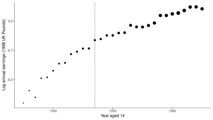
Figure 2: Average of natural logarithm of annual earnings by year aged 14. Vertical line indicates the year 1947, in which the minimum school-leaving age changed from 14 to 15. Volume of dots is proportional to share of workers in the full data with the corresponding age.

Oreopoulos (2006) studies the effect of a change in the minimum school-leaving age in the United Kingdom from 14 to 15 on schooling attainment and workers’ earnings. The change occurred in 1947 in Great Britain (England, Scotland and Wales), and in 1957 in Northern Ireland. The data are a sample of UK workers who turned 14 between 1935 and 1965, obtained by combining the 1984–2006 waves of the U.K. General Household Survey; see Oreopoulos (2006, 2008) for details.

For simplicity, we focus on the sub-sample of British workers, and restrict attention to the effect of facing a higher minimum school-leaving age on (the natural logarithm of) annual earnings measured in 1998 U.K. Pounds. Oreopoulos uses a sharp RDD to estimate this parameter. The running variable is the year in which the worker turned 14, and the treatment threshold is 1947. The running variable thus has $G=31$ support points, of which $G^{+}=19$ are above the threshold, and $G^{-}=12$ ones are below. Oreopoulos (2006, 2008) uses the global specification

$$\log(\text{EARN}_{i})=\beta_{0}+\tau\cdot\mathbb{I}\left\{\text{YEAR14}_{i}\geq 1947\right\}+\sum_{k=1}^{4}\beta_{k}\cdot\text{YEAR14}_{i}^{k}+U_{i}.$$ (6.1)

Table LABEL:tab:results4 reports the resulting treatment effect estimate along with CRV and conventional EHW standard errors and CIs for this specification (column (1)). In addition, we consider linear and quadratic specifications fitted separately on each side of the threshold using either the full data set (columns (2)–(3)), or with the estimation window restricted to $h=6$ years around the threshold (columns (4)–(5)), or $h=3$ years (columns (6)–(7)).

For Oreopoulos’ original specification in column (1), the EHW standard error is twice as large as CRV standard error. The corresponding 95% EHW CI covers zero, whereas the 95% CRV CI does not. For the linear specification using the full data in column (2), the point estimate is negative, and EHW standard errors are slightly smaller than CRV ones. Figure 2 suggests that this may be due to substantial misspecification of a global linear model below the threshold. For the remaining specifications in Table LABEL:tab:results4, all EHW standard errors are larger than the CRV standard errors, by a factor between 1.6 and 28.9. For both the linear and the quadratic specifications, the factor generally increases as the bandwidth (and thus the number of support points used for estimation) decreases. Moreover, the factor is larger for quadratic specifications than it is for the linear specifications. This is in line with the theoretical results presented in Section 4. While our analysis does not imply that EHW CIs have correct coverage in this setting, it does imply that any CI with correct coverage must be at least as wide as the EHW CI. As a result, since none of the EHW CIs in Table LABEL:tab:results4 exclude zero, for the specifications in columns (1), (3) and (5)–(7), LC’s approach leads to incorrect claims about the statistical significance of the estimated treatment effect.

Next, Table LABEL:tab:results4 reports results for a bias-reduced version of the CRV estimator developed by Bell and McCaffrey (2002), which we term CRV2, and results for CIs that combine this bias-reduction with an adjusted critical value, also due to Bell and McCaffrey (2002), which we term CRV-BM. See the supplemental material for formal definitions, and Remark 2 in Section 2 for a discussion of the performance of these CIs in simulations. While these adjustments lead to larger CIs relative to CRV, CRV-BM CIs are still smaller than EHW CIs for specifications (1) and (7), and the effect in Oreopoulos’ original specification (1) is still significant. CRV2 standard errors remain smaller than EHW standard errors in all specifications except (2).

Finally, Table LABEL:tab:results4 reports the values of the honest CIs proposed in the Section 5. It shows that the BME procedure leads to CIs that are wider than the EHW CIs. The difference is most pronounced for Oreopoulos’ original specification in column (1) and the specifications that use the full data in columns (2) and (3), due a large number of support points within the estimation window. For the estimation windows $h=6$ and $h=3$, the BME CI is only slightly wider than the EHW CIs.

We also report BSD CIs for $K\in\{0.004,0.02,0.04,0.2\}$. We use the heuristic described in Section 5.1 that fixing a value of $K$ corresponds to assuming that the true CEF does not deviate from a straight line by more than $K/8$ over a one-year interval. Given that a typical increase in log earnings per extra year in age is about 0.02, we consider $K=0.04$ and $K=0.02$ to be reasonable choices, with the other values corresponding to a very optimistic and a very conservative view, respectively. We check these choices by estimating the lower bound for $K$ using the method described in the supplemental material, which yields a point estimate equal to $0.012$, with a 95% CI given by $[0.0013,\infty)$. Except for $K=0.2$, for which the implied maximum bias is as large as $0.24$ (reflecting that this choice of $K$ is very conservative), the resulting CIs, reported in columns (8)–(11) of Table LABEL:tab:results4, are reasonably tight, and in line with the results based on EHW and BME CIs.

6.2.  Lalive (2008)

Lalive (2008) exploits a sharp discontinuity in Austria’s Regional Extended Benefit Program that was in place in 1989–1991 to study how changes in unemployment benefits affect the duration of unemployment. To mitigate labor market problems in the steel sector that was undergoing restructuring, the program extended the potential duration of unemployment benefits from 30 weeks to 209 weeks for job seekers aged 50 or older, living in one of 28 labor market districts of Austria with high steel industry concentrations. The sharp age and location cutoffs in eligibility for this program allow Lalive (2008) to exploit two separate regression discontinuity designs.

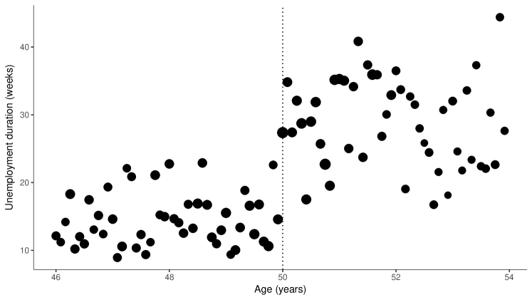
Figure 3: Average unemployment duration by age for men living in the treated districts. Vertical line indicates age 50, the cutoff for Regional Extended Benefit Program eligibility. Volume of dots is proportional to share of workers in the full data with the corresponding age.

We focus here on the design with age in months as the running variable, with 50 as the treatment threshold, and focus on the effect on unemployment duration for men aged 46–54, previously employed in non-steel sectors, living in the treated districts. Because the data used in Lalive (2008) record age only up to a precision of one month, there are $G=96$ support points, 48 above, and 48 below the cutoff. Figure 3 plots the data. Lalive (2008) uses the global polynomial regression

$$\text{DURATION}_{i}=\beta_{0}+\tau\cdot\mathbb{I}\left\{\text{AGE}_{i}\geq 50\right\}+\sum_{j=1}^{p}\beta_{j}^{-}\cdot(\text{AGE}_{i}-50)^{p}\\ +\sum_{j=1}^{p}\beta_{j}^{+}\cdot\mathbb{I}\left\{\text{AGE}_{i}\geq 50\right\}\cdot(\text{AGE}_{i}-50)^{p}+U_{i},$$ (6.2)

with $p=0,1$ or $3$, as well as a local linear regression with bandwidth $h=2$ and the Epanechnikov kernel, to estimate the parameter of interest. Lalive also reports CRV standard errors. Table LABEL:tab:lalive reproduces these estimates and standard errors, and also reports conventional EHW standard errors for these specifications (columns (1)–(4)), except in column (4) we use the uniform rather than the Epanechnikov kernel for simplicity. Columns (5)–(7) report estimates for local linear and local cubic regressions with bandwidth $h=2$ and $h=1$. Like in Section 6.1, we also report results for CRV-BM, and CRV2 that correspond to the bias-reduction modification of the CRV estimator developed by Bell and McCaffrey (2002), with and without an additional critical value adjustment.

The point estimate is relatively insensitive to changes of the specification, indicating that men stay unemployed for about 13 additional weeks in response to receiving up to 179 extra weeks of unemployment benefits. For all specifications, the EHW standard errors are bigger than CRV standard errors, by a factor of 1.1 to 2.0 that is increasing in the order of the polynomial and decreasing in the bandwidth. This is in spite of the moderate number of support points on either side of the threshold. Although the results remain significant, the CRV standard errors overestimate the precision of the results. The CRV2 adjustment does not change this conclusion. Similarly, the CRV-BM CIs are shorter than EHW CIs in all specifications considered except (5) and (7).

Table LABEL:tab:lalive also reports honest CIs proposed in Section 5. BME CIs turn out to be very wide for all specifications, and are essentially uninformative. As discussed after Proposition 2, this is because there is substantial uncertainty here about the magnitudes of the specification errors (only few observations are available for each support points, and the number of support points is relatively large). This is an instance of a setup where BME CIs are very conservative. For BSD CIs, using the heuristic from Section 5.1 that the CEF should not deviate by more than $SC/8$ over a one-year interval, we set $K=8$ and $K=16$ as reasonable choices. We also consider $K=1$ and $K=32$ as a robustness check. The specification test described in the supplemental material cannot reject linear CEF ($K=0$). Again, this is due to a relatively small number of observations available for each support point. The resulting CIs for these choices of $K$, reported in columns (8)-(11) of Table LABEL:tab:lalive, are much tighter than those based on the BME method, and quite close to the EHW CIs based local linear regression and bandwidth $h=1$.

7.  Conclusions

RDDs with a discrete running variable are ubiquitous in empirical practice. In this paper, we show that the commonly used confidence intervals based on standard errors that are clustered by the running variable have poor coverage properties. We therefore recommend that they should not be used in practice, and that one should instead proceed as follows. First, there is no need to distinguish sharply between the case of a discrete and a continuous running variable. In particular, if the discrete running variable has rich support, one can make the bandwidth smaller to reduce the bias of the treatment effect estimate, and use EHW standard errors for inference. Discreteness of the running variable only causes problems if the number of support points close to the cutoff is so small that using a smaller bandwidth to make the bias of the estimator negligible relative to its standard deviation is not feasible. Second, if one wants to deal with bias issues explicitly, one can use one of the two honest CIs described in this paper. The BSD approach works whether the running variable is discrete or continuous, whereas the BME approach is tailored to settings in which the running variable only takes on a few distinct values.

Appendix A Proofs of results in Section 4

The claims in Section 4 follow directly from general results on the properties of $\widehat{\sigma}_{\textnormal{CRV}}^{2}$ that are given in the following subsection. The proofs of these results are given in turn in Sections A.2–A.4. To state these results, we use the notation $\operatorname*{diag}\{a_{g}\}$ to denote a diagonal matrix with diagonal elements given by $a_{1},\ldots,a_{G}$, and $\operatorname*{vec}\{a_{g}\}=(a_{1}^{\prime},\ldots,a_{G}^{\prime})^{\prime}$.

A.1.  Properties of $\widehat{\sigma}_{\textnormal{CRV}}^{2}$ under General Conditions

In this subsection, we consider a setup that is slightly more general than that in Section 3, in that it also allows the bandwidth $h$ to change with the sample size. For convenience, the following assumption summarizes this more general setup.

Assumption 1 (Model).

For each $N$, the data $\{Y_{i},X_{i}\}_{i=1}^{N}$ are i.i.d., distributed according to a law $P_{N}$. Under $P_{N}$, the marginal distribution of $X_{i}$ is discrete with $G=G_{-}+G_{+}$ support points denoted $x_{1}<\dotsb<x_{G^{-}}<0\leq x_{G^{-}+1}<\dotsb<x_{G}$. Let $\mu(x)=\mathbb{E}_{N}(Y_{i}\mid X_{i}=x)$ denote the CEF under $P_{N}$. Let $\varepsilon_{i}=Y_{i}-\mu(X_{i})$, and let $\sigma^{2}_{g}=\mathbb{V}_{N}(\varepsilon_{i}\mid X_{i}=x_{g})$ denote its conditional variance. Let $h=h_{N}$ denote a non-random bandwidth sequence, and let $\mathcal{G}_{h}\subseteq\{1,\dotsc,G\}$ denote the indices for which $\lvert x_{g}\rvert\leq h$, with $G_{h}^{+}$ and $G_{h}^{-}$ denoting the number of elements in $\mathcal{G}_{h}$ above and below zero. Let $\pi_{g}=P_{N}(X_{i}=x_{g})$, $\pi=P_{N}(\lvert X_{i}\rvert\leq h)$, and $N_{h}=\sum_{i=1}^{N}\mathbb{I}\left\{\lvert X_{i}\rvert\leq h\right\}$. For a fixed integer $p\geq 0$, define

$$m(x)=(\mathbb{I}\left\{x\geq 0\right\},1,x,\ldots,x^{p},\mathbb{I}\left\{x\geq 0\right\}x,\ldots,\mathbb{I}\left\{x\geq 0\right\}x^{p})^{\prime},$$

$M_{i}=\mathbb{I}\left\{\lvert X_{i}\rvert\leq h\right\}m(X_{i})$, and $m_{g}=\mathbb{I}\left\{\lvert x_{g}\rvert\leq h\right\}m(x_{g})$. Let $\widehat{Q}=N_{h}^{-1}\sum_{i=1}^{n}M_{i}M_{i}^{\prime}$ and $Q_{N}=\mathbb{E}_{N}(M_{i}M_{i}^{\prime})/\pi$. Let $\theta_{h}=Q_{N}^{-1}\mathbb{E}_{N}(M_{i}Y_{i})/\pi$, and denote its first element my $\tau_{h}$. Let $\widehat{\theta}=\widehat{Q}^{-1}\frac{1}{N_{h}}\sum_{i=1}^{N}M_{i}Y_{i}$, and denote its first element by $\widehat{\tau}$. Define $\delta(x)=\mu(x)-m(x)^{\prime}\theta_{h}$, and $u_{i}=Y_{i}-m(X_{i})^{\prime}\theta_{h}=\delta(X_{i})+\epsilon_{i}$. Define $\Omega=\mathbb{E}_{N}(u_{i}^{2}M_{i}M_{i}^{\prime})/\pi=\sum_{g=1}^{G}(\sigma^{2}_{g}+\delta^{2}(x_{g}))Q_{g}$, where $Q_{g}=\frac{\pi_{g}}{\pi}m_{g}m_{g}^{\prime}$.

Note that the setup allows various quantities that depend on $P_{N}$ and $h$ to change with $N$, such as the number of support points $G$, their locations $x_{g}$, the conditional expectation function $\mu(x)$, or the specification errors $\delta(X_{i})$.

Assumption 2 (Regularity conditions).

(i) $\sup_{N}\max_{g\in\{1,\dotsc,G\}}\mathbb{E}_{N}(\epsilon_{i}^{4}\mid X_{i}=x_{g})<\infty$, $\det(H^{-1}Q_{N}H^{-1})=\det(\sum_{g\in\mathcal{G}_{h}}\frac{\pi_{g}}{\pi}m(x_{g}/h)m(x_{g}/h)^{\prime})>C$ for some $C>0$ that does not depend on $N$, where $H=\operatorname*{diag}\{m(h)\}$, $N\pi\to\infty$, and the limit $\lim_{N\to\infty}H^{-1}Q_{N}H^{-1}$ exists. (ii) $\sup_{N}\max_{g\in\mathcal{G}_{h}}\delta(x_{g})<\infty$; and the limit $\lim_{N\to\infty}H^{-1}\Omega H^{-1}$ exists.

The assumption ensures that that bandwidth shrinks to zero slowly enough so that the number of effective observations $N\pi$ increases to infinity, and that the number of effective support points ${G}_{h}=G_{h}^{+}+G_{h}^{-}$ is large enough so that the parameter $\theta_{h}$ and the asymptotic variance of $\widehat{\theta}$ remain well-defined with well-defined limits. We normalize $Q_{N}$ and $\Omega$ by the inverse of $H$ since if $h\to 0$, their elements converge at different rates.

Our first result is an asymptotic approximation in which $G_{h}^{+}$ and $G_{h}^{-}$ are fixed as the sample size increases. Let $B_{1},\dotsc,B_{G}$ be a collection of random vectors such that $\operatorname*{vec}\{B_{g}\}\sim\mathcal{N}(0,V)$, with

$$V=\frac{1}{\pi}\operatorname*{diag}\{\pi_{g}(\sigma^{2}_{g}+\delta(x_{g})^{2})\}-\frac{1}{\pi}\operatorname*{vec}\{\pi_{g}\delta(x_{g})\}\operatorname*{vec}\{\pi_{g}\delta(x_{g})\}^{\prime}.$$

Note that if $\lvert x_{g}\rvert>h$, then $B_{g}=0$ and $Q_{g}=0$, and that the limiting distribution of the statistic $\sqrt{N_{h}}(\widehat{\tau}-\tau_{h})$ coincides with the distribution of $e_{1}^{\prime}Q_{N}^{-1}\sum_{g=1}^{G}m_{g}B_{g}$. Finally, define

$$W_{g}=e_{1}^{\prime}Q_{N}^{-1}m_{g}\left(B_{g}-\frac{\pi_{g}}{\pi}m_{g}^{\prime}Q_{N}^{-1}\sum_{j=1}^{G}m_{j}B_{j}+(N/\pi)^{1/2}\pi_{g}\delta(x_{g})\right).$$

With this notation, we obtain the following generic result.

Theorem 1.

Suppose that Assumptions 1 and 2 hold. Suppose also that, as $N\to\infty$, (i) $G_{h}^{+}$ and $G_{h}^{-}$ are fixed; and (ii) the limit of $V$ exists. Then

$$\widehat{\sigma}_{\textnormal{CRV}}^{2} \stackrel{{\scriptstyle d}}{{=}}(1+o_{P_{N}}(1))\sum_{g=1}^{G}W_{g}^{2}.$$

Our second result is an asymptotic approximation in which the number of support points of the running variable (or, equivalently, the number of “clusters”) that are less than $h$ away from the threshold increases with the sample size.

Theorem 2.

Suppose that Assumptions 1 and 2 hold. Suppose also that, as $N\to\infty$, $G_{h}\to\infty$ and $\max_{g\in\mathcal{G}_{h}}\pi_{g}/\pi\to 0$. Then

$$\widehat{\sigma}_{\textnormal{CRV}}^{2}=(1+o_{P_{N}}(1))e_{1}^{\prime}Q_{N}^{-1}\left(\Omega+(N-1)\sum_{g=1}^{G}Q_{g}\cdot\pi_{g}\delta(x_{g})^{2}.\right)Q_{N}^{-1}e_{1}.$$

The assumption that $\max_{g\in\mathcal{G}_{h}}\pi_{g}/\pi\to 0$ ensures that each “cluster” comprises a vanishing fraction of the effective sample size.

A.2.  Auxiliary Lemma

Here we state an intermediate result that is used in the proofs of Theorem 1 and 2 below, and that shows that $\widehat{\sigma}_{\textnormal{EHW}}^{2}$ is consistent for the asymptotic variance of $\widehat{\theta}$.

Lemma 1.

Suppose that Assumptions 1 and 2 (i) hold. Then

$$\frac{N_{h}/N}{\pi} =1+o_{P_{N}}(1),$$ (A.1)

$$H^{-1}\widehat{Q}H^{-1}-H^{-1}{Q}_{N}H^{-1} =o_{P_{N}}(1).$$ (A.2)

If, in addition, Assumption 2 (ii) holds, then

$$\sqrt{N_{h}}H(\widehat{\theta}-\theta_{h})\stackrel{{\scriptstyle d}}{{=}}HQ_{N}^{-1}S+o_{P_{N}}(1),$$ (A.3)

where $S\sim\mathcal{N}(0,\Omega)$. Let $n_{g}=\sum_{i=1}^{N}\mathbb{I}\left\{X_{i}=x_{g}\right\}$, $\widehat{q}_{g}=H\widehat{Q}^{-1}Hm(x_{g}/h)\mathbb{I}\left\{\lvert x_{g}\rvert\leq h\right\}$, and $A_{g}=\frac{\mathbb{I}\left\{\lvert x_{g}\rvert\leq h\right\}}{\sqrt{N\pi}}\sum_{i=1}^{N}\left(\mathbb{I}\left\{X_{i}=x_{g}\right\}\varepsilon_{i}+(\mathbb{I}\left\{X_{i}=x_{g}\right\}-\pi_{g})\delta(x_{g})\right)$. Then $H^{-1}\sum_{g=1}^{G}m_{g}A_{g}\stackrel{{\scriptstyle d}}{{=}}H^{-1}S+o_{P_{N}}(1)$, and

$$\widehat{\sigma}_{\textnormal{CRV}}^{2}=(1+o_{P_{N}}(1))\sum_{g=1}^{G}(e_{1}^{\prime}\widehat{q}_{g})^{2}\left(A_{g}-\frac{n_{g}}{N_{h}}\widehat{q}_{g}^{\prime}\sum_{j=1}^{G}m(x_{j}/h)A_{j}+\frac{\sqrt{N}\pi_{g}\delta(x_{g})}{\sqrt{\pi}}\right)^{2}.$$ (A.4)

Furthermore, $\widehat{\sigma}_{\textnormal{EHW}}^{2}=e_{1}^{\prime}Q_{N}^{-1}\Omega Q_{N}^{-1}e_{1}+o_{P_{N}}(1)$.

Proof.

We have $\mathbb{V}_{N}(N_{h}/N)=\pi(1-\pi)/N\leq\pi/N$. Therefore, by Markov’s inequality, $N\pi\to\infty$ implies $\frac{N_{h}/N}{\pi}=\mathbb{E}_{N}(N_{h}/(N\pi))+o_{P_{N}}(1)=1+o_{P_{N}}(1)$, which proves (A.1). Secondly, since elements of $H^{-1}M_{i}$ are bounded by $\mathbb{I}\left\{\lvert X_{i}\rvert\leq h\right\}$, the second moment of any element of $\frac{N_{h}}{N\pi}H^{-1}\widehat{Q}H^{-1}-H^{-1}Q_{N}H^{-1}=\frac{1}{N\pi}\sum_{i=1}^{n}H^{-1}(M_{i}M_{i}^{\prime}-E[M_{i}M_{i}^{\prime}])H^{-1}$ is bounded by $1/(N\pi)$, which converges to zero by assumption. Thus, by Markov’s inequality, $\frac{N_{h}}{N\pi}H^{-1}\widehat{Q}H^{-1}-H^{-1}Q_{N}H^{-1}=o_{P_{N}}(1)$. Combining this result with (A.1) and the fact that $H^{-1}Q_{N}H^{-1}$ is bounded then yields (A.2).

Next note that since $\sum_{g=1}^{N}\pi_{g}m_{g}\delta(x_{g})=0$, $H^{-1}\sum_{g=1}^{G}m_{g}A_{g}=\frac{1}{\sqrt{N}}\sum_{i=1}^{N}\frac{1}{\sqrt{\pi}}H^{-1}M_{i}u_{i}$, and that by the central limit theorem, $\frac{1}{\sqrt{N}}\sum_{i=1}^{N}\frac{1}{\sqrt{\pi}}H^{-1}M_{i}u_{i}\stackrel{{\scriptstyle d}}{{=}}H^{-1}S+o_{P_{N}}(1)$. Therefore,

$$\sqrt{N_{h}}H(\widehat{\theta}-\theta_{h})=\sqrt{\frac{\pi N}{N_{h}}}(H^{-1}\widehat{Q}H^{-1})^{-1}\frac{1}{\sqrt{N}}\sum_{i=1}^{N}\frac{1}{\sqrt{\pi}}H^{-1}M_{i}u_{i}\stackrel{{\scriptstyle d}}{{=}}HQ_{N}^{-1}S+o_{P_{N}}(1),$$

as claimed. Next, we prove (A.4). Let $J_{g}=\sum_{i=1}^{N}\mathbb{I}\left\{X_{i}=x_{g}\right\}\widehat{u}_{i}M_{i}$. Then by (A.1), the cluster-robust variance estimator can be written as

$$\widehat{\sigma}_{\textnormal{CRV}}^{2}=e_{1}^{\prime}\widehat{Q}^{-1}\frac{1}{N_{h}}\sum_{g=1}^{G}J_{g}J_{g}^{\prime}\widehat{Q}^{-1}e_{1}=(1+o_{P_{N}}(1))\sum_{g=1}^{G}\left(\frac{1}{\sqrt{N\pi}}e_{1}^{\prime}\widehat{Q}^{-1}J_{g}\right)^{2}.$$

The expression in parentheses can be decomposed as

$$\begin{split}\frac{1}{\sqrt{N\pi}}e_{1}^{\prime}\widehat{Q}^{-1}J_{g}&=e_{1}^{\prime}\widehat{q}_{g}\left(A_{g}+N\pi_{g}\delta(x_{g})/\sqrt{N\pi}-n_{g}m_{g}^{\prime}(\widehat{\theta}-\theta_{h})/\sqrt{N\pi}\right)\\ &=e_{1}^{\prime}\widehat{q}_{g}\left(A_{g}+N\pi_{g}\delta(x_{g})/\sqrt{N\pi}-(n_{g}/N_{h})\widehat{q}_{g}^{\prime}H^{-1}\sum_{j=1}^{G}m_{j}A_{j}\right),\end{split}$$

which yields the result.

It remains to prove consistency of $\widehat{\sigma}_{\textnormal{EHW}}^{2}$. To this end, using (A.1), decompose

$$H^{-1}\widehat{\Omega}_{\textnormal{EHW}}H^{-1}=(1+o_{P_{N}}(1))\frac{1}{N\pi}\sum_{i=1}^{N}\widehat{u}_{i}^{2}H^{-1}M_{i}M_{i}^{\prime}H^{-1}=(1+o_{P_{N}}(1))(\mathcal{C}_{1}+\mathcal{C}_{2}+\mathcal{C}_{3}),$$

where $\mathcal{C}_{1}=\frac{1}{N\pi}\sum_{i=1}^{N}{u}_{i}^{2}H^{-1}M_{i}M_{i}^{\prime}H^{-1}$, $\mathcal{C}_{2}=\frac{1}{N\pi}\sum_{i=1}^{N}(M_{i}^{\prime}(\widehat{\theta}-\theta_{h}))^{2}H^{-1}M_{i}M_{i}^{\prime}H^{-1}$, and $\mathcal{C}_{3}=-\frac{2}{N\pi}\sum_{i=1}^{N}u_{i}M_{i}^{\prime}(\widehat{\theta}-\theta_{h})H^{-1}M_{i}M_{i}^{\prime}H^{-1}$. Since elements of $M_{i}$ are bounded by $\mathbb{I}\left\{\lvert X_{i}\rvert\leq h\right\}$, variance of $\mathcal{C}_{1}$ is bounded by $\mathbb{E}[u_{i}^{4}\mathbb{I}\left\{\lvert X\rvert_{i}\leq h\right\}]/N\pi^{2}=o_{P_{N}}(1)$, so that by Markov’s inequality, $\mathcal{C}_{1}=E[\mathcal{C}_{1}]+o_{P_{N}}(1)=H^{-1}\Omega H^{-1}+o_{P_{N}}(1)$. Similarly, all elements of $\mathcal{C}_{2}$ are bounded, $\frac{1}{N\pi}\sum_{i=1}^{N}(M_{i}^{\prime}(\widehat{\theta}-\theta_{h}))^{2}=o_{P_{N}}(1)$ by (A.1)–(A.3). Finally, $\mathcal{C}_{3}=o_{P_{N}}(1)$ by Cauchy-Schwarz inequality. Thus,

$$H^{-1}\widehat{\Omega}_{\textnormal{EHW}}H^{-1}=H^{-1}\Omega H^{-1}+o_{P_{N}}(1),$$ (A.5)

and consistency of $\widehat{\sigma}_{\textnormal{EHW}}^{2}$ then follows by combining this result with (A.2). ∎

A.3.  Proof of Theorem 1

Let ${q}_{g}=HQ_{N}^{-1}Hm(x_{g}/h)\mathbb{I}\left\{\lvert x_{g}\rvert\leq h\right\}$, and define $\widehat{q}_{g}$, $A_{g}$, and $n_{g}$ as in the statement of Lemma 1. By Lemma 1, $\widehat{q}_{g}=q_{g}(1+o_{P_{N}}(1))$, and by Markov’s inequality and Equation (A.1), $n_{g}/N_{h}=\pi_{g}/\pi+o_{P_{N}}(1)$ for $g\in\mathcal{G}_{h}$. Combining these results with Equation (A.4), it follows that the cluster-robust variance estimator satisfies

$$\widehat{\sigma}_{\textnormal{CRV}}^{2}=(1+o_{P_{N}}(1))\sum_{g=1}^{G}(e_{1}^{\prime}{q}_{g})^{2}\left(A_{g}+{\sqrt{N\pi}}\frac{\pi_{g}}{\pi}\delta(x_{g})-\frac{\pi_{g}}{\pi}{q}_{g}^{\prime}\sum_{j=1}^{G}m(x_{j}/h)A_{j}\right)^{2},$$

To prove the theorem, it therefore suffices to show that

$$e_{1}^{\prime}{q}_{g}\left(A_{g}-\frac{\pi_{g}}{\pi}{q}_{g}^{\prime}\sum_{j=1}^{G}m(x_{j}/h)A_{j}+{\sqrt{N\pi}}\frac{\pi_{g}}{\pi}\delta(x_{g})\right)=W_{g}(1+o_{P_{N}}(1)).$$ (A.6)

This follows from Slutsky’s lemma and the fact that by the central limit theorem,

$$\operatorname*{vec}\{A_{g}\} \stackrel{{\scriptstyle d}}{{=}}\operatorname*{vec}\{B_{g}\}(1+o_{P_{N}}(1)).$$ (A.7)

A.4.  Proof of Theorem 2

Throughout the proof, write $a\preceq b$ to denote $a<Cb$ for some constant $C$ that does not depend on $N$. By Equation (A.4) in Lemma 1, we can write the cluster-robust estimator as $\widehat{\sigma}_{\textnormal{CRV}}^{2}=(\mathcal{C}_{1}+\mathcal{C}_{2}+\mathcal{C}_{3})(1+o_{P_{N}}(1))$, with

$$\mathcal{C}_{1} =\sum_{g=1}^{G}(e_{1}^{\prime}\widehat{q}_{g})^{2}\left(A_{g}+(N/\pi)^{1/2}\pi_{g}\delta(x_{g})\right)^{2},$$

$$\mathcal{C}_{2} =\widehat{S}^{\prime}H^{-1}\sum_{g=1}^{G}(\widehat{q}_{g}^{\prime}e_{1})^{2}\frac{n_{g}^{2}}{N_{h}^{2}}\widehat{q}_{g}\widehat{q}_{g}^{\prime}\cdot H^{-1}\widehat{S},$$

$$\mathcal{C}_{3} =-2\sum_{g=1}^{G}(e_{1}^{\prime}\widehat{q}_{g})^{2}\left(A_{g}+(N/\pi)^{1/2}\pi_{g}\delta(x_{g})\right)\frac{n_{g}}{N_{h}}\widehat{q}_{g}^{\prime}H^{-1}\widehat{S},$$

where $\widehat{S}=\sum_{j=1}^{G}m_{j}A_{j}$, and $n_{g},A_{g}$ and $\widehat{q}_{g}$ are defined in the statement of the Lemma.

We first show that $\mathcal{C}_{2}=o_{P_{N}}(1)$. Since $H^{-1}\widehat{S}=O_{P_{N}}(1)$ by Lemma 1, it suffices to show that

$$\sum_{g=1}^{G}(\widehat{q}_{g}^{\prime}e_{1})^{2}\frac{n_{g}^{2}}{N_{h}^{2}}\widehat{q}_{g}\widehat{q}_{g}^{\prime}=o_{P_{N}}(1).$$

To this end, note that since elements of $m(x_{g}/h)$ are bounded by $1$, for any $j$, by Cauchy-Schwarz inequality, $\lvert\widehat{q}_{g}^{\prime}e_{j}\rvert\leq\lVert e_{j}^{\prime}H\widehat{Q}^{-1}H\rVert_{2}\sqrt{2(p+1)}$, where $\lVert v\rVert_{2}$ denotes the Euclidean norm of a vector $v$. By Lemma 1, $\lVert e_{j}^{\prime}H\widehat{Q}^{-1}H\rVert_{2}=O_{P_{N}}(1)$ and $N_{h}/\pi N=1+o_{P_{N}}(1)$ so that

$$\left\lvert\sum_{g=1}^{G}(\widehat{q}_{g}^{\prime}e_{1})^{2}\frac{n_{g}^{2}}{N_{h}^{2}}e_{j}\widehat{q}_{g}\widehat{q}_{g}^{\prime}e_{k}\right\rvert\leq O_{P_{N}}(1)\sum_{g\in\mathcal{G}_{h}}\frac{n_{g}^{2}}{N_{h}^{2}}=O_{P_{N}}(1)\sum_{g\in\mathcal{G}_{h}}\frac{n_{g}^{2}}{\pi^{2}N^{2}}.$$

Now, since $\mathbb{E}_{N}(n_{g}^{2})=N\pi_{g}(1-\pi_{g})+N^{2}\pi_{g}^{2}$, and $\sum_{g\in\mathcal{G}_{h}}\pi_{g}=\pi$,

$$\mathbb{E}_{N}\sum_{g\in\mathcal{G}_{h}}\frac{n_{g}^{2}}{N^{2}\pi^{2}}=\sum_{g\in\mathcal{G}_{h}}\frac{\pi_{g}(1-\pi_{g})}{N\pi^{2}}+\sum_{g\in\mathcal{G}_{h}}\frac{\pi_{g}^{2}}{\pi^{2}}\leq\left(\frac{1}{N\pi}+\frac{\max_{g\in\mathcal{G}_{h}}\pi_{g}}{\pi}\right)\sum_{g\in\mathcal{G}_{h}}\frac{\pi_{g}}{\pi}\to 0.$$

Therefore, by Markov’s inequality, $\sum_{g\in\mathcal{G}_{h}}\frac{n_{g}^{2}}{\pi^{2}N^{2}}=o_{P_{N}}(1)$, so that $\mathcal{C}_{2}=o_{P_{N}}(1)$ as claimed.

Next, consider $\mathcal{C}_{1}$. Let ${q}_{g}=HQ_{N}^{-1}Hm(x_{g}/h)\mathbb{I}\left\{\lvert x_{g}\rvert\leq h\right\}$. We have

$$\begin{split}\mathcal{C}_{1}&=\frac{1}{N\pi}\sum_{i=1}^{N}\sum_{j=1}^{N}\sum_{g=1}^{G}(e_{1}^{\prime}\widehat{q}_{g})^{2}\mathbb{I}\left\{X_{i}=x_{g}\right\}\mathbb{I}\left\{X_{j}=x_{g}\right\}(\varepsilon_{i}+\delta(x_{g}))(\varepsilon_{j}+\delta(x_{g}))\\ &=(1+o_{P_{N}}(1))\frac{1}{N\pi}\sum_{i=1}^{N}\sum_{j=1}^{N}\sum_{g=1}^{G}(e_{1}^{\prime}{q}_{g})^{2}\mathbb{I}\left\{X_{i}=x_{g}\right\}\mathbb{I}\left\{X_{j}=x_{g}\right\}(\varepsilon_{i}+\delta(x_{g}))(\varepsilon_{j}+\delta(x_{g}))\\ &=(1+o_{P_{N}}(1))\left(\mathcal{C}_{11}+2(\mathcal{C}_{12}+\mathcal{C}_{13}+\mathcal{C}_{14}+\mathcal{C}_{15}+\mathcal{C}_{16})\right),\end{split}$$

where

$$\mathcal{C}_{11} =\frac{1}{N\pi}\sum_{i=1}^{N}\sum_{g=1}^{G}(e_{1}^{\prime}{q}_{g})^{2}\mathbb{I}\left\{X_{i}=x_{g}\right\}(\varepsilon_{i}+\delta(x_{g}))^{2},$$

$$\mathcal{C}_{12} =\frac{1}{N\pi}\sum_{i=1}^{N}\sum_{j=1}^{i-1}\sum_{g=1}^{G}(e_{1}^{\prime}{q}_{g})^{2}\mathbb{I}\left\{X_{i}=x_{g}\right\}\mathbb{I}\left\{X_{j}=x_{g}\right\}\varepsilon_{i}\varepsilon_{j},$$

$$\mathcal{C}_{13} =\frac{1}{N\pi}\sum_{i=1}^{N}\sum_{j=1}^{i-1}\sum_{g=1}^{G}(e_{1}^{\prime}{q}_{g})^{2}\mathbb{I}\left\{X_{i}=x_{g}\right\}\mathbb{I}\left\{X_{j}=x_{g}\right\}\varepsilon_{j}\delta(x_{g}),$$

$$\mathcal{C}_{14} =\frac{1}{N\pi}\sum_{i=1}^{N}\sum_{j=1}^{i-1}\sum_{g=1}^{G}(e_{1}^{\prime}{q}_{g})^{2}\mathbb{I}\left\{X_{i}=x_{g}\right\}\mathbb{I}\left\{X_{j}=x_{g}\right\}\varepsilon_{i}\delta(x_{g}),$$

$$\mathcal{C}_{15} =\frac{1}{N\pi}\sum_{i=1}^{N}\sum_{j=1}^{i-1}\sum_{g=1}^{G}(e_{1}^{\prime}{q}_{g})^{2}\mathbb{I}\left\{X_{i}=x_{g}\right\}(\mathbb{I}\left\{X_{j}=x_{g}\right\}-\pi_{g})\delta(x_{g})^{2},$$

$$\mathcal{C}_{16} =\frac{1}{N\pi}\sum_{g=1}^{G}\sum_{i=1}^{N}(i-1)(e_{1}^{\prime}{q}_{g})^{2}\mathbb{I}\left\{X_{i}=x_{g}\right\}\pi_{g}\delta(x_{g})^{2}.$$

We have

$$\mathbb{E}_{N}(\mathcal{C}_{11})=\frac{1}{\pi}\sum_{g=1}^{G}(e_{1}^{\prime}{q}_{g})^{2}\pi_{g}(\sigma^{2}_{g}+\delta(x_{g})^{2})=e_{1}^{\prime}Q_{N}^{-1}\Omega Q_{N}^{-1}e_{1},$$

and

$$\begin{split}\mathbb{V}_{N}(\mathcal{C}_{11})&\leq\frac{1}{N\pi^{2}}\sum_{g=1}^{G}(e_{1}^{\prime}{q}_{g})^{4}\pi_{g}\mathbb{E}_{N}[(\varepsilon_{i}+\delta(x_{g}))^{4}\mid X_{i}=x_{g}]\preceq\frac{\sum_{g\in\mathcal{G}_{h}}\pi_{g}}{N\pi^{2}}=\frac{1}{N\pi}\to 0.\end{split}$$

Next, $\mathbb{E}_{N}(\mathcal{C}_{12})=0$, and

$$\mathbb{V}_{N}(\mathcal{C}_{12})=\frac{N-1}{2N\pi^{2}}\sum_{g=1}^{G}(e_{1}^{\prime}{q}_{g})^{4}\pi_{g}^{2}\sigma^{2}_{g}\sigma^{2}_{g}\preceq\frac{\max_{g}\pi_{g}\sum_{g=1}^{G}\pi_{g}}{\pi^{2}}=\frac{\max_{g}\pi_{g}}{\pi}\to 0.$$

The expectations for the remaining terms satisfy $\mathbb{E}_{N}(\mathcal{C}_{13})=\mathbb{E}_{N}(\mathcal{C}_{14})=\mathbb{E}_{N}(\mathcal{C}_{15})=0$, and

$$\mathbb{E}_{N}(\mathcal{C}_{16})=\frac{N-1}{2\pi}\sum_{g=1}^{G}(e_{1}^{\prime}q_{g})^{2}\pi_{g}^{2}\delta(x_{g})^{2}.$$

The variances of $\mathcal{C}_{13},\dotsc,\mathcal{C}_{16}$ are all of smaller order than this expectation:

$$\mathbb{V}_{N}(\mathcal{C}_{13}) =\frac{1}{N^{2}\pi^{2}}\sum_{g}^{G}\sum_{i,k=1}^{N}\sum_{j=1}^{\min\{i,k\}-1}(e_{1}^{\prime}{q}_{g})^{4}\pi_{g}^{3}\sigma^{2}_{g}\delta(x_{g})^{2}\preceq\frac{N\max_{g}\pi_{g}}{\pi^{2}}\sum_{g}^{G}(e_{1}^{\prime}{q}_{g})^{2}\pi_{g}^{2}\delta(x_{g})^{2}$$

$$=o(\mathbb{E}_{N}(\mathcal{C}_{16}))$$

$$\mathbb{V}_{N}(\mathcal{C}_{14}) =\frac{1}{N^{2}\pi^{2}}\sum_{i=1}^{N}\sum_{j=1}^{i-1}\sum_{k=1}^{i-1}\sum_{g=1}^{G}(e_{1}^{\prime}{q}_{g})^{4}\pi_{g}^{3}\sigma^{2}_{g}\delta(x_{g})^{2}=o(\mathbb{E}_{N}(\mathcal{C}_{16}))$$

$$\mathbb{V}_{N}(\mathcal{C}_{15}) =\frac{1}{N^{2}\pi^{2}}\sum_{i=1}^{N}\sum_{k=1}^{N}\sum_{j=1}^{\min\{i,k\}-1}\sum_{g,f=1}^{G}\left(\mathbb{I}\left\{g=f\right\}\pi_{g}-\pi_{g}\pi_{f}\right)\pi_{g}\pi_{f}(e_{1}^{\prime}{q}_{g})^{2}(e_{1}^{\prime}{q}_{f})^{2}\delta(x_{f})^{2}\delta(x_{g})^{2}$$

$$\leq\frac{1}{N^{2}\pi^{2}}\sum_{i=1}^{N}\sum_{k=1}^{N}\sum_{j=1}^{\min\{i,k\}-1}\sum_{g=1}^{G}\pi_{g}^{3}(e_{1}^{\prime}{q}_{g})^{4}\delta(x_{g})^{4}=o(\mathbb{E}_{N}(\mathcal{C}_{16})),$$

and

$$\begin{split}\mathbb{V}_{N}(\mathcal{C}_{16})&=\frac{1}{N^{2}\pi^{2}}\sum_{g=1}^{G}\sum_{f=1}^{G}\sum_{i=1}^{N}(i-1)^{2}(\mathbb{I}\left\{g=f\right\}\pi_{g}-\pi_{g}\pi_{f})\pi_{g}\pi_{f}\delta(x_{g})^{2}\delta(x_{f})^{2}(e_{1}^{\prime}{q}_{g})^{2}(e_{1}^{\prime}{q}_{f})^{2}\\ &\leq\frac{N}{\pi^{2}}\sum_{g=1}^{G}\pi_{g}^{3}\delta(x_{g})^{4}(e_{1}^{\prime}{q}_{g})^{4}=o(\mathbb{E}_{N}(\mathcal{C}_{16})).\end{split}$$

It therefore follows that

$$\mathcal{C}_{1}=(1+o_{P_{N}}(1))\mathbb{E}_{N}(\mathcal{C}_{1})=(1+o_{P_{N}}(1))\left(e_{1}^{\prime}Q_{N}^{-1}\Omega Q_{N}^{-1}e_{1}+\frac{N-1}{\pi}\sum_{g=1}^{G}(e_{1}^{\prime}q_{g})^{2}\pi_{g}^{2}\delta(x_{g})^{2}\right).$$

Finally, the cross-term $\mathcal{C}_{3}$ is $o_{P_{N}}(\mathbb{E}_{N}(\mathcal{C}_{1})^{1/2})$ by Cauchy-Schwarz inequality, so that $\widehat{\sigma}_{\textnormal{CRV}}^{2}=(1+o_{P_{N}}(1))\mathbb{E}_{N}(\mathcal{C}_{1})$, which yields the result.

Appendix B Proofs of results in Section 5

For the proof of Propositions 1, we suppose that Assumptions 1 and 2 (i) hold. We denote the conditional variance of $\tau$ by $\tilde{\sigma}^{2}_{\tau}=e_{1}^{\prime}HQ_{N}^{-1}H\tilde{\Omega}HQ_{N}^{-1}He_{1}$, where $\tilde{\Omega}=\mathbb{E}[\sigma^{2}(X_{i})\lambda(X_{i})]/\pi$, and $\lambda(x)=m(x/h)\cdot m(x/h)^{\prime}\mathbb{I}\left\{\lvert x\rvert\leq h\right\}$. We assume that $\tilde{\sigma}^{2}_{\tau}$ is bounded and bounded away from zero. To ensure that $\widehat{\sigma}^{2}_{NN}$, as defined in Section 5.1, is consistent, we assume that as $N\to\infty$, $P_{N}(\sum_{g=1}^{G_{h}}\mathbb{I}\left\{n_{g}\leq 1\right\})\to 0$, so that in large samples there are at least two observations available for each support point. We put $\widehat{\sigma}^{2}_{g}=0$ if $n_{g}\leq 1$. For simplicity, we also assume that $h\to 0$; otherwise $r_{\sup}$ will diverge with the sample size.

For the proof of Proposition 2, we suppose that Assumptions 1 and 2 hold. For simplicity, we also assume that as $N\to\infty$, $G_{h}^{+}$ and $G^{-}_{h}$ are fixed, and that $\min_{g\in\mathcal{G}_{h}}\pi_{g}/\pi$ is bounded away from zero. We also assume that the asymptotic variance of $\widehat{\tau}+\widehat{b}(W)$ is bounded away from zero for some $W\in\mathcal{W}$.

B.1.  Proof of Proposition 1

We first derive the expression for $r_{\sup}$, following the arguments in Theorem B.1 in Armstrong and Kolesár (2016). Note first that the local linear estimator $\widehat{\tau}$ can be written as a linear estimator, $\widehat{\tau}=\sum_{i=1}^{N}w(X_{i})Y_{i}$, with the weights $w(x)$ given in (5.2). Put $w_{+}(x)=w(x)\mathbb{I}\left\{x\geq 0\right\}$, and $w_{-}(x)=w(x)\mathbb{I}\left\{x<0\right\}$, and put $\mu_{+}(x)=\mu(x)\mathbb{I}\left\{x\geq 0\right\}$ and $\mu_{-}(x)=\mu(x)\mathbb{I}\left\{x<0\right\}$, with the convention that $\mu_{-}(0)=\lim_{x\uparrow 0}\mu(0)$. Since $\sum_{i=1}^{N}w_{+}(X_{i})=-\sum_{i=1}^{N}w_{-}(X_{i})=1$ and $\tau=\mu_{+}(0)-\mu_{-}(0)$, the conditional bias has the form

$$\tilde{\tau}_{h}-\tau=\sum_{i}w_{+}(X_{i})(\mu_{+}(X_{i})-\mu_{+}(0))+\sum_{i}w_{-}(X_{i})(\mu_{-}(X_{i})-\mu_{-}(0)).$$

By assumption, the first derivatives of the functions $\mu_{+}$ and $\mu_{-}$ are Lipschitz, and hence absolutely continuous, so that, by the Fundamental Theorem of Calculus and Fubini’s theorem, we can write, for $x\geq 0$, $\mu_{+}(x)=\mu_{+}(0)+\mu_{+}^{\prime}(0)x+r(x)$, and for $x<0$, $\mu_{-}(x)=\mu_{-}(0)+\mu_{-}^{\prime}(0)x+r(x)$, where $r(x)=\mathbb{I}\left\{x\geq 0\right\}\int_{0}^{x}\mu^{\prime\prime}(s)(x-s)\,ds+\mathbb{I}\left\{x<0\right\}\int_{x}^{0}\mu^{\prime\prime}(s)(x-s)\,ds$. Since the weights satisfy $\sum_{i=1}^{N}X_{i}w_{+}(X_{i})=0$, and $\sum_{i=1}^{N}X_{i}w_{-}(X_{i})=0$, it follows that

$$\begin{split}\tilde{\tau}_{h}-\tau&=\sum_{i\colon X_{i}\geq 0}w(X_{i})r(X_{i})+\sum_{i\colon X_{i}<0}w(X_{i})r(X_{i})\\ &=\int_{0}^{\infty}\mu^{\prime\prime}(s)\sum_{i\colon X_{i}\geq s}w(X_{i})(X_{i}-s)\,ds+\int_{-\infty}^{0}\mu^{\prime\prime}(s)\sum_{i\colon X_{i}\leq-s}w(X_{i})(X_{i}-s)\,ds,\end{split}$$

where the second line uses Fubini’s theorem to change the order of summation and integration. Next, note that $\bar{w}_{+}(s)=\sum_{i\colon X_{i}\geq s}w(X_{i})(X_{i}-s)$ is negative for all $s\geq 0$, because $\bar{w}_{+}(0)=0$, $\bar{w}_{+}(s)=0$ for $s\geq h$, and $\bar{w}_{+}^{\prime}(s)=-\sum_{X_{i}\geq s}w(X_{i})$ is monotone on $[0,h]$ with $\bar{w}_{+}^{\prime}(0)=-1$. Similarly, $\bar{w}_{-}(s)=\sum_{i\colon X_{i}\leq-s}w(X_{i})(X_{i}-s)$ is positive for all $s\geq 0$. Therefore, the expression in the preceding display is maximized by setting $\mu^{\prime\prime}(x)=-K\operatorname{sign}(x)$, and minimized by setting $\mu^{\prime\prime}(x)=K\operatorname{sign}(x)$. Plugging these expressions into the preceding display then gives $\lvert\tilde{\tau}_{h}-\tau\rvert\leq B_{N}$, with $B_{N}=-K\sum_{i=1}^{N}w(X_{i})X_{i}^{2}\operatorname{sign}(X_{i})/2$, which yields (5.2).

Let $o_{P_{N}}(1)$ denote a term that’s asymptotically negligible, uniformly over $\mathcal{M}_{\textnormal{H}}(K)$. To complete the proof, we need to show that (i) $\widehat{\sigma}_{NN}=\tilde{\sigma}^{2}_{\tau}+o_{P_{N}}(1)$, (ii) $\sqrt{N}_{h}(\widehat{\tau}-\tilde{\tau}_{h})=\mathcal{N}(0,\tilde{\sigma}^{2}_{\tau})+o_{P_{N}}(1)$, (iii) $\sqrt{N_{h}}(\tilde{\tau}_{h}-\tau)=b(\mu)+o_{P_{N}}(1)$, and (iv) $\sqrt{N_{h}}B_{N}=B_{\infty}+o_{P_{N}}(1)$, where $b(\mu)=\sqrt{N/\pi}\cdot e_{1}^{\prime}Q_{N}^{-1}\mathbb{E}[M_{i}r(X_{i})]$ and $B_{\infty}=-(K/2\sqrt{N/\pi})\cdot e_{1}^{\prime}Q_{N}^{-1}\mathbb{E}[M_{i}X_{i}^{2}\operatorname{sign}(X_{i})]$ are non-random, and by an argument analogous to that in the preceding paragraph, satisfy $\sup_{\mu\in\mathcal{M}_{\textnormal{H}}(K)}\lvert b(\mu)\rvert\leq B_{\infty}$. It then follows from uniform continuity of $\operatorname{cv}_{1-\alpha}(\cdot)$ that

$$P_{N}(\sqrt{N_{h}}\lvert\widehat{\tau}-\tau\rvert\leq\operatorname{cv}_{1-\alpha}(r_{\sup})\widehat{\sigma}_{NN}^{2})=P_{N}(\lvert Z+b(\mu)/\tilde{\sigma}^{2}_{\tau}\rvert\leq\operatorname{cv}_{1-\alpha}(B_{\infty}/\tilde{\sigma}^{2}_{\tau})\tilde{\sigma}^{2}_{\tau})+o_{P_{N}}(1),$$

where $Z\sim\mathcal{N}(0,1)$, from which honesty follows.

To show (i), note that by (A.1), (A.2), and the law of large numbers, it suffices to show that $H^{-1}\widehat{\Omega}_{NN}H^{-1}-N_{h}^{-1}\sum_{i=1}^{N}\sigma^{2}(X_{i})\lambda(X_{i})=o_{P_{N}}(1)$. Note that $N_{h}\widehat{\Omega}_{NN}=\sum_{i}\mathbb{I}\left\{n(X_{i})>1\right\}\cdot\epsilon_{i}^{2}\lambda(X_{i})-\sum_{i>j}\epsilon_{i}\epsilon_{j}\mathbb{I}\left\{X_{i}=X_{j},n(X_{i})>1\right\}/(n(X_{i})-1)$, where $n(x)=\sum_{j=1}^{N}\mathbb{I}\left\{X_{j}=x\right\}$ (so that $n(x_{g})=n_{g}$). This yields the decomposition

$$H^{-1}\widehat{\Omega}_{NN}H^{-1}-\frac{1}{N_{h}}\sum_{i=1}^{N}\sigma^{2}(X_{i})\lambda(X_{i})=\frac{1}{N_{h}}\sum_{i=1}^{N}(\epsilon_{i}^{2}-\sigma^{2}(X_{i}))\lambda(X_{i})\\ +\frac{(1+o_{P_{N}}(1))\cdot 2}{\sqrt{N\pi N_{h}}}\sum_{i>j}\epsilon_{i}\epsilon_{j}\frac{\mathbb{I}\left\{n(X_{i})>1\right\}\mathbb{I}\left\{X_{i}=X_{j}\right\}\lambda(X_{i})}{n(X_{i})-1}-\frac{1}{N_{h}}\sum_{i=1}^{N}\lambda(X_{i})\epsilon_{i}^{2}\mathbb{I}\left\{n(X_{i})=1\right\}.$$

Since elements of $\lambda(X_{i})$ are bounded by $\mathbb{I}\left\{\lvert X_{i}\rvert\leq h\right\}$, the first term on the right-hand side of the preceding display is of the order $o_{P_{N}}(1)$ by the law of large numbers. Conditional on $X_{1},\dotsc,X_{N}$, the second term has mean zero and variance bounded by $\frac{8}{N\pi}\max_{i}\sigma^{4}(X_{i})$, which implies that unconditionally, it also has mean zero, and variance that converges to zero. Therefore, by Markov’s inequality, it is also of the order $o_{P_{N}}(1)$. Finally, by assumption of the proposition, the probability that the third term is zero converges to one. Thus, $\widehat{\sigma}_{NN}=\tilde{\sigma}^{2}_{\tau}+o_{P_{N}}(1)$ as required.

Next, (ii) holds by (A.1), (A.2), and a central limit theorem. To show (iii), note that

$$\sqrt{N}_{h}(\tau_{h}-\tau)=(1+o_{P_{N}}(1))e_{1}^{\prime}{Q}_{N}^{-1}H\frac{1}{\sqrt{N\pi}}\sum_{i}H^{-1}M_{i}r(X_{i}).$$

Since elements of $H^{-1}M_{i}r(X_{i})$ are bounded by $\mathbb{I}\left\{\lvert X_{i}\rvert\leq h\right\}KX_{i}^{2}/2\leq\mathbb{I}\left\{\lvert X_{i}\rvert\leq h\right\}Kh^{2}/2$, it follows that elements of the variance matrix of $(N\pi)^{-1/2}\sum_{i}H^{-1}M_{i}r(X_{i})$ are bounded by $K^{2}h^{4}/4$. Thus, (iii) follows by Markov’s inequality. Finally, the proof of (iv) is analogous.

B.2.  Proof of Proposition 2

It suffices to show that for each $W\in\mathcal{W}$, the left- and right-sided CIs $[c_{L}^{1-\alpha}(W),\infty)$ and $(-\infty,c_{R}^{1-\alpha}(W)]$ are asymptotically valid CIs for $\tau_{h}+b(W)$, for any sequence of probability laws $P_{N}$ satisfying the assumptions stated at the beginning of Appendix B, and satisfying $\mu\in\mathcal{M}_{\text{BME}}(h)$. Honesty will then follow by the union-intersection principle and the definition of $\mathcal{M}_{\text{BME}}(h)$.

Note first that by the central limit theorem and the delta method,

$$\sqrt{N_{h}}\begin{pmatrix}\operatorname*{vec}(\widehat{\mu}_{g}-\mu_{g})\\ N_{h}^{-1}\sum_{i=1}^{N}H^{-1}M_{i}u_{i}\end{pmatrix}=_{d}\mathcal{N}\left(0,\;\begin{pmatrix}\pi\operatorname*{diag}(\sigma^{2}_{g}/\pi_{g})&\operatorname*{vec}(\sigma^{2}_{g}m_{g}^{\prime}H^{-1})\\ \operatorname*{vec}(\sigma^{2}_{g}m_{g}^{\prime}H^{-1})^{\prime}&H^{-1}\Omega H^{-1}\end{pmatrix}\right)+o_{P_{N}}(1).$$

Applying the delta method again, along with Lemma 1, yields

$$\sqrt{N_{h}}\begin{pmatrix}\operatorname*{vec}(\widehat{\delta}(x_{g})-\delta(x_{g}))\\ \widehat{\tau}_{h}-\tau_{h}\end{pmatrix}=_{d}\mathcal{N}\left(0,\Sigma\right)+o_{P_{N}}(1),$$

where the variance matrix $\Sigma$ is given by

$$\Sigma=\begin{pmatrix}\operatorname*{diag}(\sigma^{2}_{g}\cdot\pi/\pi_{g})+\mathcal{V}&\operatorname*{vec}(\sigma^{2}_{g}m_{g}^{\prime}Q_{N}^{-1}e_{1}-m_{g}^{\prime}Q_{N}^{-1}\Omega Q_{N}^{-1}e_{1})\\ \operatorname*{vec}(\sigma^{2}_{g}m_{g}^{\prime}Q_{N}^{-1}e_{1}-m_{g}^{\prime}Q_{N}^{-1}\Omega Q_{N}^{-1}e_{1})^{\prime}&e_{1}^{\prime}Q_{N}^{-1}\Omega Q_{N}^{-1}e_{1}\end{pmatrix},$$

and $\mathcal{V}$ is a $G_{h}\times G_{h}$ matrix with $(g,g^{*})$ element equal to $m_{g}^{\prime}Q^{-1}\Omega Q^{-1}m_{g^{*}}-(\sigma^{2}_{g}+\sigma^{2}_{g^{*}})m_{g}^{\prime}Q^{-1}m_{g^{*}}$.

Fix $W=(g^{-},g^{+},s^{-},s^{+})$, and let $a(W)\in\mathbb{R}^{G_{h}+1}$ denote a vector with the $g_{-}$th element equal to $s^{-}$, $(G_{h}^{-}+g_{+})$th element equal to $s^{+}$, the last element equal to one, and the remaining elements equal to zero. It follows that $\sqrt{N_{h}}(\widehat{\tau}+\widehat{b}(W)-\tau_{h}-b(W))$ is asymptotically normal with variance $a(W)^{\prime}\Sigma a(W)$. To construct the left- and right-sided CIs, we use the variance estimator

$$\widehat{V}(W)=a(W)^{\prime}\widehat{\Sigma}a(W),$$ (B.1)

where $\widehat{\Sigma}$ is a plug-in estimator of $\Sigma$ that replaces $Q_{N}$ by $\widehat{Q}$, $\Omega$ by $\widehat{\Omega}_{\text{EHW}}$, $\pi/\pi_{g}$ by $N_{h}/n_{g}$, and $\sigma^{2}_{g}$ by $\widehat{\sigma}_{g}^{2}$ (given in Section 5.1). Since by standard arguments $n_{g}/N_{h}=\pi_{g}/\pi+o_{P_{N}}(1)$, and $\widehat{\sigma}_{g}^{2}=\sigma^{2}_{g}+o_{P_{N}}(1)$, it follows from (A.2) and (A.5) that $\widehat{V}(W)=a(W)^{\prime}{\Sigma}a(W)+o_{P_{N}}(1)$, which, together with the asymptotic normality of $\sqrt{N_{h}}(\widehat{\tau}+\widehat{b}(W)-\tau_{h}-b(W))$, implies asymptotic validity of $[c_{L}^{1-\alpha}(W),\infty)$ and $(-\infty,c_{R}^{1-\alpha}(W)]$, as required.

Appendix C Additional Figures

This appendix shows the fit of the specifications considered in Section 2. Specifically, Figure LABEL:fig_data1a shows the fit of a linear specification ($p=1$) for the four values of the bandwidth $h$ considered; Figure LABEL:fig_data1b shows the analogous results for a quadratic fit ($p=2$). In each case, the value of the parameter $\tau_{h}$ is equal to height of the jump in the fitted line at the 40-year cutoff.

References

- Abadie and Imbens (2006) Abadie, A. and G. W. Imbens (2006): “Large Sample Properties of Matching Estimators for Average Treatment Effects,” Econometrica, 74, 235–267.
- Abadie et al. (2014) Abadie, A., G. W. Imbens, and F. Zheng (2014): “Inference for Misspecified Models with Fixed Regressors,” Journal of the American Statistical Association, 109, 1601–1614.
- Armstrong and Kolesár (2016) Armstrong, T. B. and M. Kolesár (2016): “Simple and honest confidence intervals in nonparametric regression,” ArXiv:1606.01200.
- Armstrong and Kolesár (2017) ——— (2017): “Optimal inference in a class of regression models,” ArXiv:1511.06028.
- Bell and McCaffrey (2002) Bell, R. M. and D. F. McCaffrey (2002): “Bias Reduction in Standard Errors for Linear Regression with Multi-Stage Smples,” Survey Methodology, 28, 169–181.
- Calonico et al. (2014) Calonico, S., M. D. Cattaneo, and R. Titiunik (2014): “Robust Nonparametric Confidence Intervals for Regression-Discontinuity Designs,” Econometrica, 82, 2295–2326.
- Cameron and Miller (2014) Cameron, C. A. and D. L. Miller (2014): “A Practitioner’s Guide to Cluster-Robust Inference,” Journal of Human Resources, 50, 317–372.
- Card et al. (2008) Card, D., C. Dobkin, and N. Maestas (2008): “The Impact of Nearly Universal Insurance Coverage on Health Care Utilization: Evidence from Medicare,” American Economic Review, 98, 2242–58.
- Card et al. (2015) Card, D., D. S. Lee, Z. Pei, and A. Weber (2015): “Inference on Causal Effects in a Generalized Regression Kink Design,” Econometrica, 83, 2453–2483.
- Casella and Berger (2002) Casella, G. and R. L. Berger (2002): Statistical Inference, Pacific Grove, CA: Duxbury/Thomson Learning, 2nd ed.
- Cheng et al. (1997) Cheng, M.-Y., J. Fan, and J. S. Marron (1997): “On automatic boundary corrections,” Annals of Statistics, 25, 1691–1708.
- Chetty et al. (2013) Chetty, R., J. N. Friedman, and E. Saez (2013): “Using Differences in Knowledge across Neighborhoods to Uncover the Impacts of the EITC on Earnings,” American Economic Review, 103, 2683–2721.
- Clark and Royer (2013) Clark, D. and H. Royer (2013): “The Effect of Education on Adult Mortality and Health: Evidence from Britain,” American Economic Review, 103, 2087–2120.
- Devereux and Hart (2010) Devereux, P. J. and R. A. Hart (2010): “Forced to be Rich? Returns to Compulsory Schooling in Britain,” Economic Journal, 120, 1345–1364.
- Dong (2015) Dong, Y. (2015): “Regression discontinuity applications with rounding errors in the running variable,” Journal of Applied Econometrics, 30, 422–446.
- Frandsen (2016) Frandsen, B. R. (2016): “Party Bias in Union Representation Elections: Testing for Manipulation in the Regression Discontinuity Design When the Running Variable is Discrete,” Working Paper.
- Fredriksson et al. (2013) Fredriksson, P., B. Öckert, and H. Oosterbeek (2013): “Long-term effects of class size,” Quarterly Journal of Economics, 128, 249–285.
- Gelman and Imbens (2014) Gelman, A. and G. Imbens (2014): “Why high-order polynomials should not be used in regression discontinuity designs,” NBER Working Paper.
- Gerard et al. (2016) Gerard, F., M. Rokkanen, and C. Rothe (2016): “Bounds on Treatment Effects in Regression Discontinuity Designs under Manipulation of the Running Variable, with an Application to Unemployment Insurance in Brazil,” NBER Working Paper.
- Hahn et al. (2001) Hahn, J., P. Todd, and W. van der Klaauw (2001): “Identification and Estimation of Treatment Effects with a Regression-Discontinuity Design,” Econometrica, 69, 201–209.
- Hansen (2007) Hansen, C. B. (2007): “Asymptotic properties of a robust variance matrix estimator for panel data when T is large,” Journal of Econometrics, 141, 597–620.
- Hinnerich and Pettersson-Lidbom (2014) Hinnerich, B. T. and P. Pettersson-Lidbom (2014): “Democracy, redistribution, and political participation: Evidence from Sweden 1919–1938,” Econometrica, 82, 961–993.
- Imbens and Kolesár (2016) Imbens, G. W. and M. Kolesár (2016): “Robust Standard Errors in Small Samples: Some Practical Advice,” Review of Economics and Statistics, 98, 701–712.
- Lalive (2008) Lalive, R. (2008): “How Do Extended Benefits Affect Unemployment Duration? A Regression Discontinuity Approach,” Journal of Econometrics, 142, 785–806.
- Lee and Card (2008) Lee, D. S. and D. Card (2008): “Regression discontinuity inference with specification error,” Journal of Econometrics, 142, 655–674.
- Lee and Lemieux (2010) Lee, D. S. and T. Lemieux (2010): “Regression Discontinuity Designs in Economics,” Journal of Economic Literature, 48, 281–355.
- Lemieux (2006) Lemieux, T. (2006): “Increasing residual wage inequality: Composition effects, noisy data, or rising demand for skill?” American Economic Review, 96, 461–498.
- Li (1989) Li, K.-C. (1989): “Honest confidence regions for nonparametric regression,” Annals of Statistics, 17, 1001–1008.
- Liang and Zeger (1986) Liang, K.-Y. and S. L. Zeger (1986): “Longitudinal data analysis using generalized linear models,” Biometrika, 73, 13–22.
- Low (1997) Low, M. G. (1997): “On nonparametric confidence intervals,” Annals of Statistics, 25, 2547–2554.
- MacKinnon and White (1985) MacKinnon, J. G. and H. White (1985): “Some Heteroskedasticity-Consistent Covariance Matrix Estimators with Improved Finite Sample Properties,” Journal of Econometrics, 29, 305–325.
- Martorell and McFarlin (2011) Martorell, P. and I. McFarlin (2011): “Help or hindrance? The effects of college remediation on academic and labor market outcomes,” Review of Economics and Statistics, 93, 436–454.
- Oreopoulos (2006) Oreopoulos, P. (2006): “Estimating average and local average treatment effects of education when compulsory schooling laws really matter,” American Economic Review, 152–175.
- Oreopoulos (2008) ——— (2008): “Estimating Average and Local Average Treatment Effects of Education When Compulsory Schooling Laws Really Matter: Corrigendum,” Available at http://www.aeaweb.org/articles.php?doi=10.1257/000282806776157641.
- Sacks and Ylvisaker (1978) Sacks, J. and D. Ylvisaker (1978): “Linear estimation for approximately linear models,” Annals of Statistics, 1122–1137.
- Schochet et al. (2010) Schochet, P., T. Cook, J. Deke, G. Imbens, J. Lockwood, J. Porter, and J. Smith (2010): “Standards for Regression Discontinuity Designs.” What Works Clearinghouse, Institute of Education Sciences, U.S. Department of Education.
- Urquiola and Verhoogen (2009) Urquiola, M. and E. Verhoogen (2009): “Class-size caps, sorting, and the regression-discontinuity design,” American Economic Review, 99, 179–215.