Use of Topology in physical problems

 

Some of the basic concepts of topology are explored through known physics problems. This helps us in two ways, one, in motivating the definitions and the concepts, and two, in showing that topological analysis leads to a clearer understanding of the problem. The problems discussed are taken from classical mechanics, quantum mechanics, statistical mechanics, solid state physics, and biology (DNA), to emphasize some unity in diverse areas of physics.

It is the real Euclidean space, ${\mathbb{R}}^{d}$, with which we are most familiar. Intuitions can therefore be sharpened by appealing to the relevant features of this known space, and by using these as simplest examples to illustrate the abstract topological concepts. This is what is done in this chapter.

 

 

1 The Not-so-simple Pendulum

An ideal pendulum is our first example. It is not necessarily a simple harmonic oscillator (SHO), though the small amplitude motion can be well approximated by a linear oscillator. This difference is important for dynamics, and a topological analysis brings that out.

The planar motion of a pendulum in the earth’s gravitational field is described by a generalized coordinate $q$ where $q$ is the angle $\theta$ as in Fig. 1.

1.1 Mechanics

The equation of motion (with all constants set to $1$) can be written as a second order equation or two first order equations involving the momentum $p$ as

$$\ddot{q}+\sin q=0,\ {\rm or}\ \left\{\begin{array}[]{ll}\dot{q}&=p,\\ \dot{p}&=-\sin q,\end{array}\right.$$ (1)

where a dot represents a time derivative, and the conserved energy as

$$E=\frac{1}{2}\;\dot{q}^{2}+(1-\cos q).$$ (2)

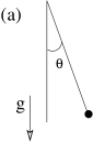
Figure 1: Planar pendulum: (a) A bob of mass $m(=1)$ is suspended by a massless rigid rod of length $L(=1)$ in a uniform gravitational field with $g(=1)$ as the acceleration due to gravity. The generalized coordinate $q$ is angle $\theta$. The configuration space for $\theta$ is (b) a circle $S^{1}$ or, (c) the real axis with equivalent points $x=x+2n\pi,n\in\mathbb{Z}$. Here ${\mathbb{Z}}$ represents the set of all integers, positive, negative, 0. We may choose $q=x$ to be the length of the arc along the circular contour. A simple harmonic oscillator corresponds to $q=x\in R$ without any equivalent point.

Let us make a list of some of the relevant results known from mechanics.

1. The potential energy has minima at $q=2n\pi$, and maxima at $q=(2n+1)\pi$, $n=0,\pm 1,...$, i.e., $n\in{\mathbb{Z}}$. These represent the stable and the unstable equilibrium points.

2. The stable motion for small energies, $E<2$, are oscillations around the minimum energy point $q=0$. Let’s call these type-O motion.

3. For larger energies, $E>2$, the motion consists of rotations in the vertical plane, clockwise or anticlockwise. These are type-R motion.

4. There is a very special critical one that separates the above two types, viz., the case with $E=2$, when $E$ is equal to the potential energy at the topmost position ($q=\pi$). Let’s call it type-C.
   The strangeness of the critical one is its infinite time period. Since most of the time is spent near the top, it looks like an inverted pendulum at the unstable equilibrium point.

5. For all problems of classical mechanics or statistical mechanics, there are two spaces to deal with, the configuration space for the set of values taken by the degrees of freedom, and the phase space, where the configuration space is augmented by the set of values of the momenta. What sort of “spaces” are these?

6. That there are three different classes of orbits cannot be overemphasized. The equation of motion is time reversible under $t\to-t,q\to q,p\to-p$. This time reversibility is respected by the type-O motion, but not by type-R because a right circular motion would go over to a left one. For type-R, the symmetry is explicitly broken by the initial conditions, which, however, do not play any crucial role for type-O.

7. As a coupled first order equations, Eq. (1), has fixed points at $q=n\pi,p=0$, which are centres for even $n$ but saddle points for odd $n$.

1.2 Topological analysis: Teaser

A topological analysis of the motion would be based on possible continuous deformations of one solution or trajectory to the other, without involving any explicit solution of Eq. 1.

Why deform? This is tantamount to asking whether there is any qualitative change in motion, as opposed to a detailed quantitative one, for a small change in energy or in the initial conditions. A small change in the amplitude of vibration due to a small change in energy is like a continuous deformation of the tajectory. In topology, the rule of deformation is to bend or stretch in whatever way we want except that neither distinct points be identified (no gluing) nor any tearing be done. Such transformations are called continuous transformations.

If the energy is changed continuously from $E_{0}$ to $E_{1}$ by defining a continuous function $E(\tau)$, say $E(\tau)=E_{0}+(E_{1}-E_{0})\tau$ with $\tau\in[0,1]$ do the trajectories in phase space get deformed continuously? The answer is not necessarily yes. This is where the global properties of the phase space or the configuration space come into play. The continuous deformations then help us both in characterizing the phase space and in classifying the trajectories. We show that the three types of motion, O, R and C belong to three different classes of curves in the appropriate phase space.

The topological analysis is done by identifying (i) the configuration space and the phase space, (ii) the possible trajectories on these spaces, and for Hamiltonian systems, (iii) the constant energy “surface” (or manifolds) for possible real motions. We do these qualitatively first and then discuss some of the features in more detail.

Figure 2: (a)The direct product phase space is a cylinder. (b) Type-1 and type-2 trajectories are marked (i) and (ii) in (b) and (c). The trajectory going completely around the circle in (b) maps to an open line in (c). Consequently any closed loop on ${\mathbb{R}}$ can be shrunk to a point. The real line is the universal cover of $S^{1}$.

1.2.1 Configuration space and phase space:

The first step is to construct the configuration and the phase spaces. The values taken by the degrees of freedom defines a set. One then defines a topology on it by defining the open sets, thereby generating the topological space to be called the configuration space. The phase space is obtained by adding the momenta variables to the configuration space.

For a pendulum, with $q$ an angle, the configuration space is a circle $S^{1}$. It is also possible to represent the configuration space as the real line ${\mathbb{R}}$ with an identification of all points $x=x+2n\pi$, $n\in\mathbb{Z}$ as in Fig. 1. The momentum, being real, trivially belongs to ${\mathbb{R}}$, the real line. The phase space is therefore $S^{1}\times{\mathbb{R}}$. The direct product phase space is the surface of a cylinder (see Fig. 2), where the radius of the cylinder is not important.

Note that the phase space can also be viewed as the extended space ${\mathbb{R}}\times{\mathbb{R}}$ with proper interpretation of one ${\mathbb{R}}$.

1.2.2 Trajectories:

Since the generalized coordinates and the conjugate momenta change continuously with time, the motion of the bob generates a curve in the phase space. This curve is called a trajectory. The second step is to construct all the possible trajectories.

As Eq. (1) is time reversible, any piece of trajectory in the upper half plane of the $(q,p)$ phase space with arrow to the right (indicating the direction of motion), has a mirror image in the lower half ($p\to-p$) with arrow towards left. As a corollary, this time-reversed pair meets to form a closed orbit, if and only if there is a point with $p=0$. In addition, uniqueness of solution for a given initial condition forbids crossing of distinct trajectories.

(a)     (b)

(c)

Figure 3: Trajectories on (a) the cylindrical phase space, and (b) the extended space ${\mathbb{R}}^{2}$. The closed orbits around $\theta=0$ in (a) are equivalent to the closed orbits around the stable points $q=2n\pi$ denoted by filled dots in (b) for $E<2$. In contrast, the closed orbits in (a) encircling the cylinder for $E>2$ correspond to the open ones in (b). The critical trajectory connects the unstable points $q=(2n+1)\pi$ represented by unfilled squares in (b) but it just encircles the cylinder in (a) with a point of contact. The U-tube space when $E$ is used as an axis is shown in (c). The actual trajectories are the $E=$const plane intersections of the U-tube. On the right, three different types of intersections: closed for $E<2$ (topologically equivalent to a circle $S^{1}$), figure 8 for $E=2$ (two circles with one common point, called the wedge sum $S^{1}\vee S^{1}$), and two disconnected closed pieces for $E>2$ (disjoint union of two circles, $S^{1}\cup S^{1}$ but with $S^{1}\cap S^{1}=\emptyset$ ).

Let us now combine all the above features. We find that the possible trajectories in the extended ${\mathbb{R}}^{2}$ space are either closed loops around $q=2n\pi$ or open curves. See Fig. 3. There is the transitional one that connects the saddle points at $q=(2n+1)\pi$ at $p=0$. On the cylindrical phase space, all are closed orbits; one type (for $E<2$) enclosing the stable fixed point $(0,0)$, and another type encircling the cylinder (with $E>2$). The latter can be grouped into two inequivalent classes, namely the time reversed partners (see item 6 in Sec. 1.1). It is obvious that one type cannot be deformed into the other one if we follow the rules of deformation on the cylinder. The special one is $E=2$, a conjoined twin connected at one point. It requires a pinching (i.e., identification) of two points on the curve for $E<2$. A tearing is required as $E$ exceeds 2 by any amount no matter how small. Moral: The topology of the phase space naturally separates the three types of orbits. The cylindrical topology forbids transformation of one to the other.

Another way to see the change is to use energy $E(p,q)$ as a parameter or replace $p$ by $E$. As $E$ depends quadratically on $p$, the cylindrical phase space becomes a U-tube. To be noted that the horizontal $p=0$ circle on the cylinder has now become the vertical circle in the middle of the U as the minimum energy is zero for $\theta=0$ but 2 for $\theta=\pi$. The motion is then given by the intersection of the U-tube with an $E=$const plane. See Fig. 3. The three classes of closed loops are now easy to see. The corresponding orbits in the configuration space are shown in Fig. 2.

The peculiarity of the critical case is revealed by the response of the pendulum to a vanishingly small random perturbation at say the turning or the top point. There will be no drastic change for the $E>2$ or the $E<2$ cases. But for the figure eight case, when $E=2$, the motion would consist of any combination of clockwise (C) and anticlockwise (A) orbits like CCAAAACACCC… . That is to say, all infinitely long two letter words are possible trajectories, and any two words differing in at least one letter are distinct.

Problem 1.1:

Suppose acceleration due to gravity $g=0$. The phase space is still a cylinder but the motion is different. Discuss how the topological arguments change, by focusing on the change in the U-tube for energy as $g\to 0$.

2 Topological analysis: details

We now discuss how topology is used in the description. Let us remember that a topology on a set $X$ of points require a set of subsets, $\tau$, to be called open sets, such that (i) $\emptyset{}$ (Null set) and full set $X$ are open, i.e., $\emptyset{},X\in\tau$, (ii) any finite or infinite union of open sets is also open, (iii) any finite intersection of open sets, i.e. members of $\tau$, belongs to $\tau$. Under these conditions, the set of subsets, $\tau$, is called a topology on $X$, while $(X,\tau)$ is said to constitute a topological space. See Ref. [4].

A useful procedure to define a topology on a set is to embed it in a known space. Then use the intersections of the open sets of the known space with the set in hand to define the open sets in it. For example, $S^{1}$ can be drawn in a two dimensional space and the open sets on this curve can be defined as the intersection of the curve with the rectangles (or Disks). The open sets on the circle then form the basis for the topology on $S^{1}$. The topology thus defined is called the Inherited topology or the subspace topology. Since we shall mostly be working with these inherited topologies, we shall not be explicit about it anymore, unless something else is meant. Such embeddings are useful in most physics problems but there are many cases for which no embeddings are possible.

Right now we rely on our intuition of spaces.

2.1 Configuration Space

Our familiarity with the real $d$-dimensional Euclidean space $R^{d}$ allows us the luxury of thinking of other spaces in terms of $R^{d}$. With that, it might be possible to make topological identifications of spaces. There should be a statutory warning that proving the topological equivalence of spaces in general could be a notoriously difficult problem.

2.1.1 $S^{1}$ as the configuration space

Our intuition of angle leads us naturally to $S^{1}$. If we think of the set of values $q\in[0,2\pi]$, we get $S^{1}$ only if we identify $0$ and $2\pi$. This can be seen by gluing the two ends of a piece of a string (i.e. implement the “periodic boundary condition”). A simple but concrete way of seeing this is to note that a continuous map takes $q\to z=e^{iq}$ with $z$ defining the unit circle in the complex plane.

2.1.2 ${\mathbb{R}}$ as the configuration space: equivalence relation, quotient space

A slightly different identification is required for the extended real line used in Fig. 1. This involves an equivalence relation that any $x\in{\mathbb{R}}$ is equivalent to all points $x+na$ for $n\in Z$. It is like a translational symmetry in one dimension. Any point on ${\mathbb{R}}$ can then be brought into the interval $[0,a]$ or $[-a/2,a/2]$ by addition or subtraction of suitable multiples of $a$. E.g., $-a/2=a/2-a$ sets $-a/2$ as equivalent to $a/2$. This finite closed interval with end point identification is $S^{1}$. If the equivalence is denoted by the symbol $\sim$, i.e. $x\sim x+na$, then under this equivalence condition, the relevant space is different from $\mathbb{R}$. It is denoted by ${\mathbb{R}}/\!\!\sim$, and is called the quotient space for the equivalence relation $\sim$. The space obtained via an equivalence as ${\mathbb{R}}/\!\!\sim$ is topologically equivalent to $S^{1}$. A general feature we see here is the possibility of construction of new spaces from a given space by defining an equivalence relation on it.

More examples

For the closed interval $I=[0,1]$, we may define the periodic boundary condition as an end point equivalence relation $0\sim 1$. Then $I/\!\!\sim$ is homeomorphic to $S^{1}$, where homeomorphism is synonymous to “topologically identical”. To be more systematic, one defines (i) a direct map (i.e. a function) $f:I\to S^{1}$ as $f(x)=e^{i2\pi x}$, and successive maps (ii) a map $f_{1}:I\to I/\!\sim$, and (iii) an inverse map $f_{2}:I/\!\sim\,\,\to S^{1}$, so that $f_{2}(f_{1}(x))=f(x)$ for all $x\in I$.

Note that, we do not get $S^{1}$ from $[0,1]$ if the end points are not identified. That they are different can be seen by removing one point from each one of the two sets. In the closed interval case we get two disconnected pieces whereas for $S^{1}$ we get an open interval. If we take an open interval like $q\in(0,1)$, then it is actually equivalent to the whole real line as one may verify by the map $x\to X=\tan[\pi(x-\frac{1}{2})]$ with $X\in(-\infty,+\infty)$.

Problem 2.1:

The change in the topological space by an equivalence relation has important consequences in physics too. Take the case of $[0,1]$ and $S^{1}$ under the equivalence condition. For single particle quantum mechanics, the first case corresponds to the boundary condition where the wave function $\psi(x)=0$ at $x=0,1$ while the second one to periodic boundary condition with $\psi(0)=\psi(1)$.

Take the conventional momentum operator $-i\hbar d/dx$ with the eigen value equation $-i\hbar\frac{d\psi}{dx}=p\psi$. Show that there is no valid solution (i.e., $p$ is not real) for the $[0,1]$ case while $p$ is real for $S^{1}$.

2.1.3 Pendulum vs harmonic oscillator:

The importance of the topology of the configuration space can be understood by comparing the $S^{1}$ case with the space for the linearized simple pendulum. For the latter, the configuration space is just a small part of the circle (small angles), which can be extended to the whole real line as for a linear harmonic oscillator. For this space ${\mathbb{R}}$, there is only one stable fixed point at $x=0$, and the phase space has only one kind of orbit, namely the closed orbit of libration type. All the richness of the full pendulum at various energies come from the nontrivial topology of the configuration space.

2.2 Phase space

Now that we know the configuration space, we may go over to the phase space. The momentum part is easy - it is a real number for the pendulum, $p\in(-\infty,+\infty)$, i.e. $p\in{\mathbb{R}}$. For $n$ degrees of freedom there are $n$ momenta, and so the space for the momenta is ${\mathbb{R}}\times{\mathbb{R}}...\times{\mathbb{R}}={\mathbb{R}}^{n}$. Since the momentum and the position are independent variables, we have a product space of ${\mathbb{R}}^{n}\times C$ where $C$ is the configuration space, as seen for the planar pendulum.

The motion of the pendulum is restricted to the constant energy subspace of the phase space as shown in Fig. 3. Beyond visualization, the differences in the nature of the spaces show up through their topological invariants, e.g., by the fundamental group.

2.2.1 Topological invariants — homotopy groups:

One way of exploring a topological space $X$ is by mapping known spaces like circles, spheres, etc in $X$. The case with circles tells us how many classes of nonequivalent closed loops that start and end at a point $x_{0}$ can exist in $X$. Any point in $X$ can be chosen as the base point $x_{0}$. Two loops that can be deformed into one another are called homotopic[5]. All such homotopic loops can be clubbed together as a single class, with any one of them as a representative one. One may also define a product of two loops $C_{1}$ and $C_{2}$ by going along $C_{1}$ and then from $x_{0}$ along $C_{2}$. There will be classes of loops that are homotopic to $C$, and therefore the multiplication is for the classes. Representing a class by $[\gamma]$ for all loops homotopic to $\gamma$, the multiplication rule can be written as $[C]=[C_{2}]\;[C_{1}]$. An inverse of a loop $C$ can be defined as the loop traversed in the opposite direction, so that $C\;C^{-1}$ is homotopic to a point (i.e. a trivial loop). More formally, all these imply that the closed loops rooted at $x_{0}$ form a group under the opration of loop multiplications. This group is called the fundamental group of $X$, $\pi_{1}(X,x_{0})$. For a connected space, i.e. if any two points can be connected by a path in $X$, the special point, the base point can be chosen arbitrarily. We shall therefore drop $x_{0}$ from the notation.

The fundamental group of the space for $E<2$ is $\pi_{1}(``E<2")=\mathbb{Z}$ where the base point has been dropped. This part of the space is like the outer surface of a bowl. In contrast, the space for $E>2$ is disjoint – two tubes, and the loops will depend on whether the base point, $x_{0}$, is in one or the other circle. Although $\pi_{1}(``E>2",x_{0})=\mathbb{Z}$, but $x_{0}$ in one circle cannot be connected by a path to the point on the other. Such a disjoint set is characterized by the zeroth homotopy group $\pi_{0}(``E>2")=\{-1,1\}\equiv{\mathbb{Z}_{2}}$ with two elements signifying two components. The critical surface is again two circles but with one common point forming figure 8. Such a union of spaces with one common point is called a wedge sum, indicated by a $\vee$. This fundamental group is now a nonabelian group $\pi_{1}(``E=2")=\mathbb{Z}\star\mathbb{Z}$ a free group of two elements.

The difference in the fundamental group tells us that the spaces are not identical, i.e., not homeomorphic.

Problem 2.2:

Show that a square with periodic boundary conditions is equivalent to $S^{1}\times S^{1}$. Take a piece of paper and glue the sides parallelly. This is a torus which is associated with two holes. Define the appropriate equivalence relation ($\sim$), and convince yourself that the compact notation is $[0,1]\times[0,1]/\!\sim\,=S^{1}\times S^{1}$. This “=” means “homeomorphic” or loosely speaking “topologically equivalent”.

We have already seen two spaces formed by two circles in the case of a pendulum. Compared to the disconnected space with $\pi_{0}=\{-1,1\}$, a torus has $\pi_{0}=0$, just as figure 8 which we obtained from two circles with one point equivalence. Both (torus and figure 8) are connected spaces. That a torus is not topologically figure 8 is established by $\pi_{1}(S^{1}\times S^{1})=\mathbb{Z}\times\mathbb{Z}$ while $\pi_{1}({\rm figure\ 8})=\mathbb{Z}\star\mathbb{Z}$.

Problem 2.3:

Discuss the connection between the fundamental groups of the constant energy spaces mentioned above and the real trajectories of the pendulum.

Problem 2.4:

The phase space for a simple harmonic oscillator is $\mathbb{R}^{2}$ with $\pi_{1}(\mathbb{R}^{2})=0$. Discuss the motion with respect to the corresponding $E$-$x$ surface.

Problem 2.5:

The energy of a free one-dimensional quantum particle is given by $E_{k}=ak^{2}$ with the wavevector $k\in{\mathbb{R}}$. The state with the wavefunctin described by $k$ may called left-moving or right moving for $k<0$ or $k>0$. For a particle on a lattice (lattice spacing=1), the translational symmetry makes two $k$ values equivalent if they differ by a reciprocal lattice vector. In other words the $k$-space is like Fig. 1c. The equivalence relation makes the relevant space $S^{1}$ as in Fig. 1b. A linear representation of $S^{1}$ is the interval $[-\pi,\pi]$ with the identification of the two end points. With this identification, a right moving particle at $k=\pi$ becomes a left moving particle at $k=-\pi$ as defined earlier, but one should keep in mind the presence of reciprocal lattice vectors . Draw $E_{k}$ vs $k$ in this 1st Brillouin zone.

Problem 2.6:

(a) Argue that the configuration space of the pendulum in full space (spherical pendulum) is $S^{2}$ (surface of a three dimensional sphere). (b) Discuss the possible types of motions using topological arguments. (c) In spherical coordinates $S^{2}$ can be described by $(\theta,\phi)$ where $\theta\in I=[0,\pi]$, and $\phi\in[0,2\pi]$. Why is $S^{2}$ not a product space $I\times S^{1}$?

Problem 2.7:

If all the boundary points of a square are made equivalent, then it is topologically equivalent to a surface of a sphere $S^{2}$. Take a piece of cloth or paper and use a string to bring all the boundary points together, as one does to make a bag. Or take a square and an isolated point. Connect all the points on the boundary to that point.

Problem 2.8:

Bloch’s theorem, in solid state physics, is generally proved for a lattice with periodic boundary conditions, i.e., on a torus (an $n$-torus for an $n$-dimensional crystal. E.g., a torus is obtained by identifying opposite edges of a square. Note that if all points on the boundary of a square are identified (spherical boundary condition) one gets $S^{2}$. Is Bloch’s theorem valid for the spherical boundary condition? Are the reciprocal vectors defined for the spherical boundary condition?

Problem 2.9:

Bulk and edge states: In the tight binding model, a quantum particle hops on a square lattice. Find the energy eigen states under the following situations. Pay attention to bulk and edge states. (i) A particle on $S^{1}\times S^{1}$. In this case there are only bulk states. (ii) With spherical boundary condition, i.e., on $S^{2}$. There are no edges. But are the bulk states same as in (i)? (iii) Klein Bottle. No edges but different from (i) and (ii). (iv) Periodic boundary condition in one direction, i.e., on a finite cylinder. There are now two edges. (v) Antiperiodic boundary condition, i.e., a Möbius strip. There is now one single edge.

Problem 2.10:

Argue that the configuration space for the planar motion of a double pendulum is $S^{1}\times S^{1}$. If we consider the full three dimensional space, then the configuration space is $S^{2}\times S^{2}$.

Problem 2.11:

A classical Hamiltonian system with $n$ degrees of freedom is integrable if there exists $n$ conserved quantities or “first integrals”. In such a case, the motion is confined on an $n$-torus $S^{1}{\times...\times}S^{1}$. Here the product space indicates that the motions can be handled independently. This is easy to see in the action angle variables where the $n$ angles constitute the $n$-tori. Convince yourself about this for the pendulum case and for the well-known Kepler problem. This result is useful in the context of the important KAM theorem.

Problem 2.12:

Kapitza Pendulum: The linearized equation of motion around the vertical inverted position of a pendulum under a periodic vertical drive is $\ddot{\theta}-(g+a(t))\theta=0$ where $a(t)=a(t+\tau)$ is the periodic vertical modulation of the point of suspension. The inverted pendulum is stable if the amplitude of the drive exceeds some critical value. This is called a Kapitza pendulum. Discuss the motion of an inverted pendulum under a periodic vertical drive vis-a-vis Fig. 3.

Problem 2.13:

Show that a plane with a hole is equivalent (homeomorphic) to a cylinder. With the hole as the origin, use polar coordinates $r,\phi$ so that $r=0$ is excluded (=hole). Now do a mapping $r\to X=\ln r$ so $X\in(-\infty,+\infty)$, i.e., $X\in{\mathbb{R}}$ and $\phi$ defines $S^{1}$. Therefore ${\mathbb{R}}^{2}-\{0\}$ (also written as ${\mathbb{R}}^{2}\\{0\}$) is a cylinder.

Solve the free particle quantum mechanics problem in ${\mathbb{R}}^{2}-\{0\}$ in $r,\phi$ coordinates. What are the boundary conditions? Do the same on the cylinder by transforming the Schrödinger equation to $X,\phi$ variables. The main point of this exercise is to see the importance of one missing point that changes the topology of the space.

Problem 2.14:

Show that a sphere with a hole $S^{2}\$N (N=north pole) is equivalent to a plane. The formal proof is by stereographic projection. A sphere with two holes (north and south poles) is like a cylinder, which in turn is a plane with a hole. What about a sphere with three missing points?

Problem 2.15:

What is the advantage of going from the cylinder to the extended real plane as in Fig. 3? The real line or plane has the special feature that any closed loop can be shrunk to a point. Such a space is called simply-connected (as opposed to multiply-connected as in the previous problem). A practical usefulness may be seen by considering a damped pendulum described by $\ddot{\theta}+\gamma\dot{\theta}+\sin\theta=0,$ where $\gamma$ is the friction coefficient. Now energy is not conserved, $dE/dt<0$, so that the pendulum ultimately for $t\to\infty$ comes to rest at the stable fixed point $\theta=0$. Draw the possible trajectories (phase portrait) of this damped pendulum for different values of $\gamma$ and starting energy ($E>2,E<2$) both on the cylinder and on the extended space.

3 Topological spaces

Is the combination of two real variables $q,p$ equivalent to a two dimensional Euclidean plane? The question arises because even if we take $q$, and $p$ as the two directions of the xy plane, still we may not be in a position to define a distance between two points $(q_{1},p_{1})$ and $(q_{2},p_{2})$. The second point is that for a physical system described by two variables, the state space may locally be like a plane (two dimensional) but different global connectivities may imply important qualitative differences. E.g., for a torus and a sphere, a small neighbourhood of a point may be described by the tangent plane at that point and would look simmilar, but globally they are different. Let us concentrate on the first issue now.

The absence of a metric (or distance) is a generic problem we face whenever we want to draw a graph of two different parameters. Take, for example, a plot of pressure $P$ and volume $V$ for a verification of Boyle’s law. The plot reassuringly gives us a branch of a hyperbola, which is defined as the locus of a point such that the difference in the distance from two fixed points remain constant. But it would be ridiculous to define an Euclidean distance between $(P_{1},V_{1})$ and $(P_{2},V_{2})$. Still, we know, graph plotting does work marvelously.

The identification is done in steps through topology. First an appropriate topological space is defined which can be identified with the similar topological space in ${\mathbb{R}}^{2}$. Then, use the equivalence of this topological space and a metric or distance based ${\mathbb{R}}^{2}$.

Let’s start with the real line. To define a topology we need a list or a definition of open sets. Let’s define all sets of the type $(a,b),(b>a)$ and their unions as open sets. The null set $\emptyset{}$ and the full set are also members of the set of open sets. That these subsets form a topology on ${\mathbb{R}}$ is easy to check. The set of subsets with the union and intersection rules then defines a topological space. For the real line we used only the “greater than” or “less than” relation, without defining any distance or metric.

Figure 4: Basis for $R^{2}$ as a topological space: open rectangles or disks.

This topology can be extended to ${\mathbb{R}}^{2}={\mathbb{R}}\times{\mathbb{R}}$ by defining the sets of open rectangles $(a_{1},a_{2})\times(b_{1},b_{2})$. See Fig. 4. By doing this we defined a topology in $\mathbb{R}^{2}$ without using any distance. The next step is to define a metric, the usual Euclidean distance in ${\mathbb{R}}^{2}$ with which open disks $D=(x,y|(x-a)^{2}+(y-b)^{2}<\epsilon)$ can be defined around a point $(a,b)$. It is known that the topology defined by the open rectangles and their unions is the same as the one defined by the disks.

By this procedure, with the help of boxes, the $(q,p)$ phase-space can be taken as a topological space equivalent to ${\mathbb{R}}^{2}$. This equivalence allows one to see all the geometric features of ${\mathbb{R}}^{2}$ in the graphs we plot or in the phase space, without explicitly defining the distance.

An important feature of the topology of the phase space is that it is connected and simply connected, i.e. one may go from any point to any other point, and any two paths connecting two points can be deformed into each other. A connected phase space is nice because that is a sufficient condition for the applicability of equlibrium statistical mechanics (generally called ergodicity - that one can go from any state to any other). However, a phase space may as well be in disconnected pieces in the sense that two parts may be separated by infinite energy barriers. Such spaces might be relevant for phase transitions where the phase space may get fragmented into pieces (“broken ergodicity” or ordered systems).

Problem 3.1:

In Fig. 4, an infinite number of open boxes are used as “basis” sets to define the topology of ${\mathbb{R}}^{2}$. As a vector space, we need only two unit vectors ${\bf i,j}$ where the number $2$ of ${\mathbb{R}}^{2}$ determines the number of basis vectors. Where is this “2” when defined as the topological space? Argue that this dimensionality comes from the number of spaces required to construct the boxes.

Problem 3.2:

We defined the topology for $S^{1}$ by embedding it in $\mathbb{R}^{2}$ (subspace topology). Is it possible to define a topology on $S^{1}$ without any embedding?

Figure 5: (a) A double well potential. (b) A double well potential but with an infinite barrier inbetween. The barrier cannot be crossed.

Problem 3.3:

Consider the one-dimensional motion of a particle in a double well $V(x)=\frac{1}{2}K(x^{2}-a^{2})^{2}$. See Fig.5(a). Discuss the nature of the configuration space and of the phase space. Locate the fixed points and draw the phase space portrait.

Problem 3.4:

Suppose the barrier of the double well potential is infinitely high (Fig. 5b.) Argue that the configuration space consists of disconnected pieces. Draw the possible phase portraits.

4 More examples of topological spaces

Let us now consider a few other well-known spaces used in condensed matter physics. Once the spaces are identified, their topological classifications in terms of fundamental groups and higher homotopy groups help us in identifying the defects that may occur, the type of particles that may be seen and so on. Here we just construct the spaces in a few cases.

A class of condensed matter systems involve ordered states. like crystals, magnets, liquid crystals, etc. These states or phases have a symmetry described by a group $H$ which is a subgroup of the expected full symmetry $G$. For example, the Hamiltonian of $N$ interacting particles is expected to be invariant under full translational and rotational symmetry, $G$, but a crystal, described by the same Hamiltonian has only a discrete set of space group symmetries. Such phenomena of ordering is known as symmetry breaking. The ordered state is then described by a parameter that reflects this subgroup structure of the state. The allowed values of the order parameter constitutes the topological space for the ordered state and this space is called the order parameter space. Of all the ordered states, ferromagnets and liquid crystals are easy to describe. We discuss these spaces below.

4.1 Magnets

A ferromagnet is described by a magnetization vector ${\bf M}$. In the paramagnetic phase ${\bf M}=0$ but a ferromagnet by definition has ${\bf M}\neq 0$. For simplicity (e.g. at a particular temperature or zero temperature) we take $M=$const , only its direction may change.

Magnets can be of different types depending on the nature of the vector. If ${\bf M}$ takes only two directions up or down, then it is to be called an Ising magnet. If ${\bf M}$ is a two dimensional vector, it is an xy magnet, and for a three dimensional vector it is an Heisenberg magnet. In the ferromagnetic phase the origin ($M=0$) is not allowed and so any vector space description will be of limited use. What is then required is a topological description of the allowed values of the magnetization. Since ferromagnetism is a form of ordering of the microscopic magnetic vectors, we call the space an order parameter space ${\cal O}$.

It is now straightforward to see that the order parameter spaces ${\cal O}$ are of the following kinds:
(i) Ising: ${\cal O}=Z_{2}$, (0,1) i.e. up or down
(ii) xy: ${\cal O}=S^{1}$ (circle), i.e., the angle of orientation, $\theta$.
(iii) Heisenberg: ${\cal O}=S^{2}$ (surface of a 3-dimensional sphere), i.e., angle of orientation, i.e., $\theta,\phi$.
(iv) n-vector model: there are situations where the space could be $S^{n},n>2$.

If we take a macroscopic $d$-dimensional magnet, then at each point of the sample (${\bf x}\in{\mathbb{R}}^{d}$) we define a magnetization vector ${\bf M(x)}$ or a mapping ${\bf M}:{\mathbb{R}}^{d}\to{\cal O}$. That such a mapping can be nontrivial has important implications. Instead of a fullfledged analysis of the mapping, it helps to see how loops and spheres in real space map to the orderparameter space. E.g., when we move along a closed loop in real space, the order parameter describes a closed loop in ${\cal O}$. The nature of these closed loops in ${\cal O}$ is given by the fundamental group $\pi_{1}({\cal O})$. A nontrivial $\pi_{1}$ indicates there are loops that cannot be shrunk to a point. This, in turn, means that if a loop in real space is shrunk, there will be problems with continuous deformation of the spins; there has to be a singularity where the orientation of the spin cannot be defined. These are called topological defects. In $d=2$, loops will enclose point defects while in $d=3$, loops will enclose line defects, with the elements of $\pi_{1}({\cal O})$ as the “charges” of these defects.

We just quote here the results[5] that $\pi_{1}(S^{1})=\mathbb{Z}$, and $\pi_{1}(S^{n})=0,n>1$. These mean that only for the xy-magnet there will be point defects in two dimensions and line defects in three dimensions. In particular, Heisenberg magnets will have no point (line) defects in two (three) dimensions. Any Heisenberg spin configuration in real space can be changed to any other by local rearrangements of spins. In contrast, for a 2-dimensional xy magnet, a configuration with a point defect of say charge=1 cannot be converted by local rearrangements of the spins to a defectless configuration. The question of continuity of a mapping (i.e. a function) using topology is discussed separately in Sec. 6.

Problem 4.1:

There seems to be an obsession for $S^{n}$, but that’s not for no reason. Prove that $S^{n}$ is the only compact simply-connected “surface” in $n$-dimensions ($n\geq 2$). (Poincaré’s conjecture.)

Problem 4.2:

Berezinskii-Kosterlitz-Thouless transition: it is known that the cost to create a unit charge defect in the 2-d xy model is $\varepsilon\ln L$ for, say, a square lattice of size $L\times L$. Since the defect can be anywhere on the lattice, argue that the free energy of a single defect at temperature $T$ is $f(T)=\varepsilon\ln L-cT\ln L$, where $c$ is some constant. Take the defect free state as of zero free energy. Show that free defects may form spontaneously if $T>T_{\text{B}KT}=\varepsilon/c$. This phase transition is called the Berezinskii-Kosterlitz-Thouless (BKT transition).

4.2 Liquid crystals

4.2.1 Nematics: $\mathbb{R}P^{2}$

Lest we created the impression that the world is just $S^{n}$’s, we look at a different ordered system, namely liquid crystals. A nematic liquid crystal consists of rod like molecules where the centres of the rods are randomly distributed as in a liquid but the rods have a preferred orientation ${\bf N}$. This looks like a magnet but it isn’t so because a rod does not have a direction, i.e. it is like a headless arrow. A flipping of a rod won’t change anything in contrast to ${\bf M}\to-{\bf M}$. As a direction in 3-dimensions, the order parameter space ${\cal O}_{\rm nematic}$ should have been $S^{2}$ but not exactly. Two points on a sphere which are diametrically opposite represent the same state, and therefore there is an equivalence relation on the sphere that antipodal points are equivalent, ${\bf N}\to-{\bf N}$. This is not just the hemisphere but a hemisphere with the diametrically points identified on the equator. This is called the real projective plane $S^{2}/Z_{2}={\mathbb{R}}P^{2}$. In general, $S^{n}/Z_{2}={\mathbb{R}}P^{n}$.

As an ordered system, we would like to know how the headless arrows can be arranged in space. This requires the behaviour of the map ${\bf N}:{\mathbb{R}}^{d}\to{\mathbb{R}}P^{2}$.

4.2.2 Biaxial nematics

Instead of rod like molecules, one may consider rectangular parallelepiped with $2$-fold rotational symmetry corresponding to the $2\pi$ rotations around the three principal axis. Such a liquid crystal is called a biaxial nematics. The order parameter space is the sphere $S^{2}$ with the equivalence relation, $\sim$, under the three rotations. This ”$\sim$” is not just the identification of the antipodal points but, in addition, the equivalence of four sets of points (corners of the box) on the surface of the sphere. The generic notation ${\cal O}=S^{2}/\!\!\sim$ is too cryptic to have any use. This is where the symmetry operations as a group is useful.

The sphere is actually a representation of the rotational symmetry. If ${{n}}_{1},{{n}}_{2}$ are any two allowed values of the order parameter, they are related by the three dimensional rotation group $G=SO(3)$. By keeping any one value fixed, say ${{n}}_{1}$, all others can be generated by the application of the group elements of $G$. However, the special symmetry of the biaxial nematics, a subgroup of four elements, $H=D_{2}$, keeps the order parameter invariant, i.e., if $h\in H$, then $n_{1}=hn_{1}$. Then, there is some $g\in G$, for which $n_{2}=gn_{1}=ghn_{1}$, so that $n_{2}$ is generated by all group elements of the type $gh$ with $h\in H$ and $g\in G$ but not in $H$. What we get is the coset of $H$ in $G$, $G/H$. So, instead of the generic representation as $S^{2}/\!\sim$, we may use groups to represent the order parameter space as a coset space, ${\cal O}=SO(3)/D_{2}$. The similarity of notations (quotient space in topology and coset space in group theory) is not accidental but is because of the similarity of the underlying concepts. It is now straightforward to generalize to any other point group symmetry. It will be the corresponding coset space.

Problem 4.3:

Instead of $SO(3)$, one may consider $SU(2)$. Under this mapping, show that $D_{2}$ goes to a eight member nonabelian group, $Q$, the group of quaternions. Therefore, ${\cal O}=SU(2)/Q$.

Problem 4.4:

Show that the order parameter spaces for magnets can be written in terms of groups as the following coset space:

1. the xy case: ${\cal O}=SO(2)$, or ${\cal O}=U(1)$. Note that the coset space is a group in this case.

2. the Heisenberg case: ${\cal O}=SO(3)/SO(2)$, or ${\cal O}=SU(2)/U(1)$.

4.2.3 What is ${\mathbb{R}}P^{n}$?

A real projective space is obtained by identifying the points which differ by a scale factor. If any point ${\bf x}\in{\mathbb{R}}^{n+1}$ is equivalent to $\lambda{\bf x}$ for any real $\lambda\neq 0$, then under this equivalence relation $({\mathbb{R}}^{n+1}\\{0\})/\!\sim={\mathbb{R}}P^{n}$. Geometrically, all points on a straight line through the origin are taken as equivalent. The space then consists of unit vectors ${\bf n}$ with ${\bf n}$ equivalent to $-{\bf n}$.

Problem 4.5:

What is the configuration space of a rigid diatomic molecule in 3 dimensions?
Ans: ${\mathbb{R}}^{3}$ for the centre of mass and $S^{2}$ for orientation of the molecule. In case the two atoms are identical then it is ${\mathbb{R}}^{3}\times{\mathbb{R}}P^{2}$.

Figure 6: (a) Twist a circle which brings two antipodal points together. Then fold the two circles so that again antipodal points are on top of eachother. (b) The space of all lines through origin. Any point on a line, except the origin, are equivalent to all others on the same line. This space is $S^{1}$.

${\mathbb{R}}P^{1}$:

Take a circle and identify the diametrically opposite points. See Fig. 6a. This is easy to do with a rubber band. The folding process shows that $S^{1}/Z_{2}={\mathbb{R}}P^{1}=S^{1}$. Another way of looking at $RP^{1}$ is shown in Fig. 6b. Take all straight lines through origin in two dimensions. Then declare all points on a line, except the origin, as equivalent. We may choose any point (not origin) on a line as a representative point. Draw a circle through the origin with the center on the y-axis. Every line meets this circle at a point (again exclude the origin) which can be taken as a representative point of the line. There is therefore one-one correspondence between the points on the circle and the lines through the origin. The excluded point on the circle (the origin of ${\mathbb{R}}^{2}$) can then be included as the representative point for the x-axis. Hence the topological equivalence of ${\mathbb{R}}P^{1}$ and $S^{1}$.

In contrast, ${\mathbb{R}}P^{2}$ is not simple. In the Euclidean case any two straight lines intersect at one and only one point, unless they are parallel. Parallel lines do not intersect. In the real projective plane, any two straight lines always intersect either in the finite plane or at infinity.

4.3 Crystals

Take the case of a crystal which has broken translational symmetry. If we move an infinite crystal by a lattice vector, the new state is indistinguishable from the old one. For concreteness let us take the crystal to be a square lattice of spacing $a$ in the xy plane. Consider the atoms to be slightly displaced from the chosen square lattice. Now, if one atom is at ${\bf r}_{0}$ from one particular lattice site, it is at ${\bf r}_{mn}={\bf r}_{0}+ma\hat{i}+na\hat{j}$ from a site at $(m,n)$. All of these are equivalent. The order parameter space is then the real plane ${\mathbb{R}}^{2}$ under the equivalence condition of translation of a square lattice. There is now an equivalence relation that any point ${\bf r}$ is equivalent to a point ${\bf r}+ma\hat{i}+na\hat{j}$ for $m,n\in{\mathbb{Z}}$. The order parameter space is therefore a torus. Note that this is a generalization of the one dimensional case of Fig. 2 to 2-dimensions, except that we are now going from Fig 2c to Fig. 2b.

4.4 A few Spaces in Quantum mechinics

We consider the forms of a few finite dimensional Hilbert spaces.

4.4.1 Complex projective plane $\mathbb{C}P^{n}$

In quantum mechanics, the square integrable wave functions form a Hilbert space. Any state $|\psi\rangle$ can be written as a linear combination of a set of orthonormal basis set $\{|j\rangle\}$ as $|\psi\rangle=\sum_{j}c_{j}\,|j\rangle$. Let’s keep the number of basis vectors finite, $n<\infty$. The set of $n$ complex numbers $\{c_{j}\}$ is an equivalent description of the state so that the state space is an $n$-dimensional complex space ${\mathbb{C}}^{n}$. Since only normalized states matter, $\{c_{j}\}$ and $\{\lambda c_{j}\}$ for any complex number $\lambda$ represent the same state. Hence there is an equivalence relation $\{c_{j}\}\sim\{\lambda c_{j}\}$ in $\mathbb{C}^{n}$. The relevant space for wave functions is then $(\mathbb{C}^{n}{\}\{0\})/\!\!\sim\,=\mathbb{C}P^{n-1}$, a complex projective space in analogy with real projective spaces.

4.4.2 Two state system

A particular case, probably the simplest, is a two level system (a qubit), like a spin 1/2 state with $|+\rangle$ and $|-\rangle$ states. The space of states is therefore the one-dimensional complex projective plane $\mathbb{C}P^{1}$. Any normalized state can be written as

$$|\psi\rangle=\cos\frac{\theta}{2}\;\;|+\rangle+e^{i\phi}\sin\frac{\theta}{2}\;\;|-\rangle,\;\;{\rm with\;\;}0\leq\theta\leq\pi,0\leq\phi\leq 2\pi.$$ (3)

The two angular parameters $\theta$ and $\phi$ allow us to map ${\mathbb{C}}P^{1}$ to $S^{2}$, called the Bloch sphere, though there are problems with the representation of $|+\rangle$ and $|-\rangle$. To get rid of this problem one actually needs two maps. From the equivalence relation $(c_{1},c_{2})\sim(\lambda c_{1},\lambda c_{2})$, we may choose $\lambda$ to write $(c_{1},c_{2})\sim(1,z)$ or $(c_{1},c_{2})\sim(1/z,1)$ so that the two original basis vectors $|\pm\rangle$ come from $z=0$ or $z=\infty$. The addition of the point at infinity to the complex plane gives us the Riemann sphere, also called one point compactification of the complex plane.

The sphere allows us to define a metric in terms of $\theta,\phi$, which then acts as a metric, the Fubini-Study metric, for $\mathbb{C}P^{1}$.

4.4.3 Space of Hamiltonians for a two level system

The Hamiltonian for a two state system is a $2\times 2$ Hermitian matrix. Therefore we may consider the space of all such Hamiltonians. Any Hermitian $2\times 2$ matrix can be expressed in terms of the Pauli matrices

$$H=\left(\begin{array}[]{ll}\epsilon_{1}&a-ib\\ a-ib&\epsilon_{2}\end{array}\right)=\frac{\epsilon_{1}+\epsilon_{2}}{2}\mathbb{I}+a\;\sigma_{x}+b\;\sigma_{y}+\frac{\epsilon_{1}-\epsilon_{2}}{2}\;\;\sigma_{z}.$$ (5)

In general, the space of the $2\times 2$ Hermitian Hamiltonians is a real four dimensional space with $({\mathbb{I}},\sigma_{x},\sigma_{y},\sigma_{z})$ as the basis vectors.. It has to be a real space because hermiticity requires all the four numbers, $\epsilon_{1},\epsilon_{2},a,b$ to be real.

In some situations a further reduction in the dimensionality of the space is possible. By a shift of origin, we may set $\epsilon_{1}=-\epsilon_{2}=\epsilon$ to make $H$ traceless. In this situation,

$$H={\bf d}\cdot{\bf\sigma}=|d|{\bf n}\cdot{\bf\sigma},$$ (6)

with ${\bf n}={\bf d}/|d|$, a unit vector. The set of all such traceless Hamiltonians can be described by the vector ${\bf n}$, provided $|d|\neq 0$. Therefore, the space of the Hamiltonians of any two level system is $S^{2}$. The center of the sphere corresponds to the degenerate case, $|d|=0$, when the two energy eigenvalues are same.

A practical example is a spin-$1/2$ particle in a magnetic field with $H=-{\bf h}\cdot{\bf{\sigma}}$, where $h$ may depend on some external parameters including time. Another example is a two band system. For a one dimensional lattice, consider two bands $\epsilon_{1}(k),\epsilon_{2}(k)$ with some symmetry such that $\epsilon_{1}+\epsilon_{2}=$const for all $k$. Choosing the constant to be zero, we now have Hamiltonian of the type Eq. 6 with ${\bf d}(k)$ a function of the quasimomentum $k$, where $k$ is in the first Brillouin zone, $-\pi\leq k\leq\pi$. We therefore have a map $S^{1}\to S^{2}$. In two dimensions, the Brillouin zone is a torus and therefore we need to study the map ${\mathbb{T}}^{2}\to S^{2}$. Some aspects of these maps are considered in Sec. 7.7.

Problem 4.6:

Construct the topological space for the Hamiltonian of a three level system. Explain why it is reasonable to expect $SU(3)$ and not a spin $s=1$ state. Generalize it to $m$-level system for any $m$.

Problem 4.7:

The Bloch sphere describes the pure states. The density matrix of a state $|\psi\rangle$ is $\rho=|\psi\rangle\;\langle\psi|$, with $\rho^{2}=\rho,\ {\rm Tr}\ \rho=1$. These two conditions on $\rho$ can be taken as the definition of a pure state without any reference to wave functions. In this scheme, mixed states are those for which ${\rm Tr}\ \rho=1$, but $\rho^{2}\neq\rho$. This means $P={\rm Tr}\ \rho^{2}<1$. $P$ is called the purity of the state. For the two state system, mixed states are given by $2\times 2$ Hermitian, positive semidefinite matrices with trace 1. Show that these mixed states are points inside the Bloch sphere. The relevant space is now a 3-ball (a solid sphere).

5 Disconnected space: Domain walls

Of all the order parameter space for a magnet defined in Sec 4.1, the Ising class is special because here the space is disconnected. The same result is obtained by using the $\phi^{4}$ theory with an energy functional

$$E[\phi(x)]=\int_{-\infty}^{\infty}dx\ \left[\frac{1}{2}\left(\frac{d\phi}{dx}\right)^{2}+\frac{1}{2}K\left(\phi(x)^{2}-\phi_{0}^{2}\right)^{2}\right],$$ (7)

so that the minimum energy states correspond to $\phi(x)=\pm\phi_{0}$. For finite energy states, we require $\phi(x)$ to be nonconstant but going to $\pm\phi_{0}$ as $x\to\pm\infty$. The requirement at infinity gives us four possibilities, shown in a tabular form below.

	$\phi|_{x\to-\infty}$	$\phi|_{x\to\infty}$
(a)	$\phi_{0}$	$\phi_{0}$
(b)	$-\phi_{0}$	$-\phi_{0}$
(c)	$-\phi_{0}$	$\phi_{0}$
(d)	$\phi_{0}$	$-\phi_{0}$

Table 1: Boundary conditions at $\pm\infty$.

These four cases are distinct because there is no continuous transformation that would change one to the other.

For cases (a) and (b), local changes (like spin flipping) can reduce the energy to zero and these represent small deviations from the fully ordered uniform state of $\phi_{0}$ or $-\phi_{0}$. These two states are related by symmetry but they are distinct.

For cases (c) and (d), no continuous local transformation can change the boundary conditions to the uniform state. Therefore, they represent different types of states. These finite energy states are called topological excitations because their stability is protected by topology. This is a domain wall or interface separating the two possible macroscopic state $\pm\phi_{0}$. These topological excitations are called kink for (c) and anti-kink for (d).

More generally for any discrete or disconnected configuration space, i.e., if its $\pi_{0}$ (zeroth hommotopy) is nontrivial, there will be domain walls. A better description of a disconnected space is via the zeroth homology, $H_{0}$, for which we refer to Ref. [6].

Figure 7: Four possible boundary conditions for an Ising magnet with spins=$\pm 1$. The up (down) arrow indicates spin $+1(-1)$. An interface exists for (c) and (d).

One may see this boundary condition induced domain walls in the ordered state of a two dimensional Ising model on a square lattice. If we take a long strip with four different boundary conditions as in Fig. 7 along one direction, we force domain walls in cases with opposite boundary conditions as in Fig. 7c,d. The energy of the interface is obtained by subtracting the free energy of (a) or (b) from (c) or (d). This is ensured in Eq. (7) by taking the energy at infinity to be zero.

Problem 5.1:

Use the energy functional of Eq. (7) to determine the domain wall energy.

Problem 5.2:

The previous discussion allows for only one type of domain wall to exist in a configuration. A generalization would be to consider a case of several disconnected pieces of the configuration space, as in the Potts model. In this model, each “spin” can take $q$ discrete values. A lattice Hamiltonian with nearest neighbour interaction can be of the form $H=-J\sum_{nn}\delta(s_{i},s_{j}),J>0$. Show that the ground state is $q$-fold degenerate. Discuss the nature of domain walls or kinks/antikinks in the Potts model.

Problem 5.3:

The boundary conditions in Fig. 7 can be classified as periodic (a,b) and antiperiodic (c,d). If we join the two vertical edges (equivalence relation) in a way that matches the arrows, show that we get a cylinder for (a) and (b) while a Mobius strip for (c) and (d). See Appwndix A for a problem on flux thorugh such surfaces.

6 Continuous functions

So far our focus has been on the topological spaces defined for various sets. In the process functions are also defined as maps between two given spaces. It is necessary to define a continuous function in topology without invoking the $\epsilon,\delta$ definitions of calculus.

The topological definition of a continuous function is in terms of its inverse function. A function $f:A\to B$ is continuous if $f^{-1}$ maps open sets of $B$ to open sets of $A$. The definition in calculus is that given any $\epsilon$ no matter how small, if we can find a $\delta(\epsilon)$, which depends on $\epsilon$, such that $|f(x+\delta)-f(x-\delta)|<\epsilon$, then $f(x)$ is continuous at $x$. In this $\epsilon$-$\delta$ definition, continuity is linked to closeness as measured by a distance-like quantity. The topological definition replaces the neighbourhoods by the open sets, the constituent blocks of the space, but, in addition, it involves the inverse function. That should not be a surprise if we recognize that, by specifying $\epsilon$ for $f$ and then finding $\delta$ for $x$ is like generating the inverse function.

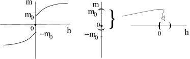
Figure 8: A discontinuous function. Magnetization vs magnetic field for a ferromagnet. At $h=0,m=0$ and $\lim_{h\to 0\pm}m(h)=\pm m_{0}$. The example on the right shows an open interval $(-\epsilon,m_{1}),\epsilon>0,m_{1}>m_{0}$, maps on to a semiclosed interval $[0,h_{1})$ for $h$, with $m(h_{1})=m_{1}$. The inverse function maps an open interval of $m$ to a semi-open interval of $h$.

We illustrate this with the help of a known physical example, namely the magnetization of a ferromagnet in a magnetic field, $m(h)$ with $m,h\in\mathbb{R}$. See Fig 8. Take any open set $(h_{i},h_{f})$. The corresponding values of $m$ form an open set $(m(h_{i}),m(h_{f}))$, missing the “discontinuous” nature at the origin. In contrast, the inverse image of $(-\epsilon,m_{1})$ maps to the semiopenset $[0,h_{1})$.

The definition of continuity in terms of the inverse image has implications in physical situations too. The response function, susceptibility, defined as $\chi=\frac{\partial m(h)}{\partial h}$ loses its significance at $h=0$. The relevant quantity in this situation is the inverse susceptibility $\chi^{-1}$ which may be defined as $\frac{\partial h(m)}{\partial m}$ in terms of the inverse function $h(m)$. In thermodynamics or statistical mechanics, the inversion is done by changing the ensemble. In a fixed magnetic field ensemble, the free energy $F(h)$ is a function of $h$ while in a fixed magnetization ensemble the free energy ${\cal F}(m)$ is a function of the magnetization. These two free energies are related in thermodynamics by a Legendre transformation. By generalizing to free energy functionals, the two response functions are defined as

$$\chi({\bf r},{\bf r}^{\prime})=\frac{\partial m({\bf r})}{\partial h({\bf r}^{\prime})}=-\frac{\delta^{2}F}{\delta h({\bf r})\;\delta h({\bf r}^{\prime})},\quad\chi^{-1}({\bf r},{\bf r}^{\prime})=\frac{\partial h({\bf r})}{\partial m({\bf r}^{\prime})}=\frac{\delta^{2}{\cal F}}{\delta m({\bf r})\;\delta m({\bf r}^{\prime})},$$ (8)

such that $\int\chi^{-1}({\bf r,r^{\prime}})\ \chi({\bf r^{\prime},r^{\prime\prime}})d{\bf r}^{\prime}=\delta({\bf r}-{\bf r}^{\prime\prime})$. Such inverse response functions lead to vertex functions in field theories.

Problem 6.1:

Consider a field theory like the $\phi^{4}$ theory of Eq. (7), defined in a $d$-dimensional space. Show that the two point vertex function for this field theory corresponds to an inverse response function.

7 Quantum mechanics

A few examples of use of topology in elementary quantum mechanics are now discussed. These examples are not to be viewed in isolation but in totality with all other examples discussed in this chapter We shall mix classical examples here too to show the broadness of the topological concepts and topological arguments. Later on these ideas in the quantum context will be connected to another, completely classical, arena of biology involving DNA.

7.1 QM on multiplyconnected spaces

We now consider quantum mechanics on topologically nontrivial spaces in quantum mechanics, for which we need to reexamine two traditional statements, namely,

1. Wave functions are single valued.

2. An overall phase factor, $\psi(x)\to e^{i\phi}\psi(x)$ does not matter.

The singlevaluedness criterion gets translated in the path integral formulation as the sum over all paths in the relevant configurational space with weights determined by the action along the path. These are actually valid for simply-connected spaces, but not necessarily for a multiply-connected space. An example of such a case is the problem of a single particle on a ring which is discussed in some detail, avoiding a full fledged general analysis. The result can be extended to the case of a plane with a hole (See Prob. 2.13) as we shall do below.

7.2 Particle on a ring

A particle is constrained to move on a ring (a circle) of circumference $L$. We use the coordinate $x$ to denote the position on the ring.

For a circle $S^{1}$ and its universal cover $\mathbb{R}$, refer to Fig. 1b,c and Fig  2b,c. To maintain generality, we use notations $\mathbb{F}$ and $\widetilde{\mathbb{F}}$ as the topological space in question, and its universal cover respectively. These are related by $\mathbb{F}=\widetilde{\mathbb{F}}/G$, where $G$ is a discrete group expressing the equivalence relations. For the ring, $\mathbb{F}=S^{1}$, and $\widetilde{\mathbb{F}}={\mathbb{R}}$, and $G=\mathbb{Z}$ (See Sec. 2.1). The requirement that $\pi_{1}(\widetilde{\mathbb{F}})=0$, sets $\pi_{1}(\mathbb{F})=G$.

A trivial loop in $\mathbb{F}$, see Fig. 2, maps to a loop in $\widetilde{\mathbb{F}}$, whereas all nontrivial loops in $\mathbb{F}$ become open paths in $\widetilde{\mathbb{F}}$. A point $q$ in $\mathbb{F}$ maps to many points (all equivalent) in $\widetilde{\mathbb{F}}$. Let us choose one such point $\widetilde{q}_{0}$ arbitrarily. A closed loop $C$ in $\mathbb{F}$ from $q_{0}$ to $q_{0}$ maps to a unique path $\widetilde{C}$ in ${\widetilde{\mathbb{F}}}$ from ${\widetilde{q}}_{0}$ to another equivalent point ${\widetilde{q}}^{\prime}_{0}$. The end point is the same for all paths homotopic to $C$ (i.e. deformable to $C$). By denoting all such homotopic paths by $[C]$ or $[\widetilde{C}]$ as the case may be, we write ${\widetilde{q}}^{\prime}_{0}=[C]\;{\widetilde{q}}_{0}$, without using any tilde on $C$.

It is now reasonable to expect

$$\widetilde{\psi}([C]\widetilde{q})=a([C])\;\widetilde{\psi}(\widetilde{q}),$$ (9)

with $a$ as a phase factor. Two loops $C,C^{\prime}$ in $\mathbb{F}$ based at $q_{0}$ can be combined into one, $[C^{\prime\prime}]=[C^{\prime}]\;[C]$. In $\widetilde{\mathbb{F}}$ the corresponding paths $\widetilde{C}$ connects $\widetilde{q}_{0}$ to $[C]\widetilde{q}_{0}$ while the subsequent $\widetilde{C}^{\prime}$ connects $[C]\widetilde{q}_{0}$ to $[C^{\prime}][C]\widetilde{q}_{0}$ which is also $[C^{\prime\prime}]\widetilde{q}_{0}$. For the wavefunction, we get the combination rule for the phase factors as

$$a([C^{\prime}])a([C])=a([C^{\prime}]\;[C])=a([C^{\prime\prime}]),$$ (10)

i.e., $a$’s follow the group multiplication rules of $\pi_{1}$. These $a$’s therefore constitute a one-dimensional representation of the fundamental group.

A simple path in $\mathbb{F}$ connects any point $q$ to $q_{0}$. Simple here means the path shrinks to a point as $q\to q_{0}$. Such paths allow us to map all the points of $\mathbb{F}$ to a domain containing $\widetilde{q}_{0}$ in $\widetilde{\mathbb{F}}$. For the circle case, this is reminiscent of a unit cell in $\mathbb{R}$. The equivalence relation or the nontriviality of $G$ suggests that there are other equivalent domains, as many as the number of elements of $G$. As an example, in Fig. 1 , the domains can be chosen as $(-\pi,\pi],(\pi,3\pi]...$, an infinite of them as $\mathbb{Z}$ is countably infinite. The wavefunction is single valued in each of these domains but those in two different domains differ by a phase factor. As any of these domains is isomorphic to ${\mathbb{F}}$, any one of these wavefunctions can be taken as the wavefunction on $\mathbb{F}$. We end up with a multivalued wavefunction on $\mathbb{F}$ whose branches are the wavefunctions on the “unit cells” of $\widetilde{\mathbb{F}}$. In short, quantum mechanics on a multiply connected space requires a multivalued wavefunction, unlike the simple cases studied in Euclidean spaces. This, fortunately, is not the end of the story. With the help of examples, we shall see that we may still choose single valued wavefunction, at the cost of an extra phase though. This is Berry’s phase which goes beyond topology and appears in many problems as a geometrical phase

Let us consider a few special cases.

7.2.1 $a=1$: single-valued wavefunction

The identity representation is the trivial representation of any group. Let us choose $a=1$ for all elements of $G=\mathbb{Z}$. The free particle Hamiltonian

$$H=\frac{p^{2}}{2m},\quad{\rm with\ }H\psi(x)=E\ \psi(x),\quad{\rm and\;\;\;}\psi(0)=\psi(L).$$ (11)

The periodic boundary condition, which incorporates our requirement of $a=1$, gives the known energy eigenfunctions and eigenvalues as

$$\psi_{k}(x)=e^{ikx}.\quad k=\frac{2\pi n}{L},n\in\mathbb{Z},\ {\rm and}\ E_{n}=\frac{2\pi^{2}\hbar^{2}n^{2}}{mL^{2}}.$$ (12)

Importantly, the wavefunction is single-valued.

7.2.2 $a_{n}=e^{in\theta}$: multi-valued wavefunction

Let us now consider the case of multivalued wavefunction. By using gauge transformation, the multivaluedness is linked to the behaviour of a particle when the ring is threaded by a magnetic flux. A connection between the two problems is then obtained via Berry’s phase.

A. Multi-valuedness

Let us choose, respecting Eq. (10), a unitary representation

$$a_{n}=e^{in\theta},n\in\mathbb{Z},$$ (13)

It is, as per Eq. (9), equivalent to a twisted boundary condition

$$\psi(0)=e^{-i\theta}\psi(L),$$ (14)

thereby making the wavefunction multivalued.

The energy eigenvalues and eigenfunctions are still given by Eq. (12) but with

$$k=\frac{2\pi n+\theta}{L},\ {\rm and}\ E_{n}=\frac{2\pi^{2}\hbar^{2}(n+n_{0})^{2}}{mL^{2}},\quad n\in\mathbb{Z},$$ (15)

where $n_{0}=\theta/(2\pi)$.

B. Gauge transformation, magnetic flux

We may do a gauge transformation for the wavefunction, $\Psi(x)=e^{i\Theta(x)}\psi(x)=U\psi(x)$, where $U$ is the unitary transformation operator. Such a transformation changes the boundary condition to

$$\Psi(L)=e^{i\Theta(L)}\psi(L)=e^{i\Theta(L)}e^{i\theta}\psi(0)=e^{i\Theta(L)}e^{-i\Theta(0)}e^{i\theta}\Psi(0).$$ (16)

The choice

$$\Theta(L)-\Theta(0)=-\theta,\ {\rm or}\ ,\Theta(x)=-\frac{\theta}{L}x,$$ (17)

gives us a $\theta$-independent boundary condition, $\Psi(L)=\Psi(0)$ as in Sec. 7.2.1. Moreover, a direct substitution shows that $\Psi(x)$ is the eigenfunction of a transformed Hamiltonian but with the same energy,

$$H_{\theta}=e^{i\Theta(x)}He^{-i\Theta(x)}=\frac{1}{2m}\left(p+\frac{\hbar\theta}{L}\right)^{2},\quad{\rm and}\quad H_{\theta}\Psi_{n}(x)=E_{n}\Psi_{n}(x),$$ (18)

where $E$ is given by Eq. (15) The quantum problem turns out to be equivalent to a charged particle in a magnetic vector potential, but with a $\theta$-independent periodic boundary condition for the wave function.

Suppose there is a thin solenoid of radius $b$ carrying a magnetic field $B$ at the center of the ring in a direction perpendicular to the plane of the ring . There is no magnetic field on the ring but there exists a vector potential

$$A=\frac{B\pi b^{2}}{2\pi r},$$ (19)

on a circle of radius $r$ in the angular direction. The Hamiltonian of a particle of charge $q$ is then $H_{mag}=\frac{1}{2m}(p-qA/c)^{2}$, $c$ being the velocity of light. Comparing this form with Eq. (18), we see that $\theta=2\pi\frac{\Phi}{\Phi_{0}}$, where $\phi_{0}=2\pi\hbar q/c$, the standard flux quantum if the charge $q$ is the electronic charge $e$.

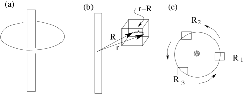
Figure 9: (a) A particle on a ring threaded by a flux line through origin. (b) A box, confining the particle, centered on ${\bf R}$ on the circle. The position of the particle inside the box is ${\bf r}$. (c) The boxed is taken around the full circle adiabatically in a continuous manner, or, say, in three steps so as to enclose the flux.

It needs to be recognized at this point that the circular ring per se is not special here; geometry does not matter. The analysis is valid for a two dimensional plane threaded by an impenetrable thin flux line, which is like a hole (See Prob. 2.13). Phase $\theta$ is independent of path, allowing us to claim that it is topological in nature. This phase is known as the Aharonov-Bohm phase.

7.3 Topological/Geometrical phase

The extra phase we derived in the preceding case is not the only one. Such phases occur in many situations, classical or quantum. For waves in classical physics, such a phase is called the Pancharatnam phase while in quantum mechanics it is Berry’s phase. As an angle it can be found in classical problems as Hannay angle, writhes in DNA and so. Often the angle may be geometric in origin, not necessarily topological. What it means is the the angle one gets may depend on the path chosen unlike the path independence of a topological quantity. In this respect it is important to distinguish between a geometrical phase and a topological phase.

7.3.1 Berry’s phase

We established the equivalence of two QM problems, viz.,

1. a charged particle on a ring enclosing a constant flux, with single valued wave function,

2. a particle on a ring in zero flux but with a multivalued wave function.

This equivalence raises the following question,

What is the analogue of the extra phase (case 2) responsible for the multivaluedness in the singlevalued version of case 1?

The answer lies in Berry’s phase.

7.3.2 Phase – an Angle: two formulas

In order to see the emergence of the phase, let us take a wavepacket localized on the ring. One way to achieve this is to enclose the particle in a small box centered on a point on the ring, and then move the box around the circle. Let the box position (centre of the box) be ${\bf R}$ on the ring. The particle is now described by

$$\left[\frac{1}{2m}\left(p-\frac{qA({\bf r})}{c}\right)^{2}+V({\bf r}-{\bf R})\right]\chi({\bf r},{\bf R})={\cal E}\chi({\bf r},{\bf R}),$$ (20)

where $A({\bf r})$ is given by Eq. (19). Within the finite-sized box the wavefunction is single valued.

Now this box is taken adiabatically around the circle through a complete turn as shown in Fig 9. We assume that the wave function changes very slowly, though, in fact, we shall see that the speed doe not matter. For two positions ${\bf R}_{1},{\bf R}_{2}$, the phase difference is defined as

$$\exp({-i\phi_{12}})=\frac{\langle\chi({\bf r},{\bf R}_{1})|\chi({\bf r},{\bf R}_{2})\rangle}{|\langle\chi({\bf r},{\bf R}_{1})|\chi({\bf r},{\bf R}_{2})\rangle|},\;\;{\rm or\;\;}\phi_{12}=-{\rm Im}\;\ln{\langle\chi({\bf r},{\bf R}_{1})|\chi({\bf r},{\bf R}_{2})\rangle}.$$ (21)

This phase between two points is somewhat arbitrary because it can be changed by a gauge transformation at any one of the points ${\bf R}_{1}$ or ${\bf R}_{2}$. In spite of this arbitrariness, it can be combined with the phases from the remaining steps to define an overall phase as (${\bf r}$ is suppressed in the notation)

$$\gamma=-{\rm Im}\ln\left({\langle\chi({\bf r},{\bf R}_{1})|\chi({\bf r},{\bf R}_{2})\rangle}{\langle\chi({\bf r},{\bf R}_{2})|\chi({\bf r},{\bf R}_{3})\rangle}.{\langle\chi({\bf r},{\bf R}_{3})|\chi({\bf r},{\bf R}_{1})\rangle}\right)$$ (22)

Note that the arbitrariness of phases at the intermediate points get cancelled in the product. Consequently the total phase $\gamma$ modulo $2\pi$ is a phase that cannot be removed by a gauge transformation, and, as a gauge invariant quantity, must have physical consequences. This phase is an example of what is called Berry’s phase.

We may take a continuum limit where the closed loop is traversed by infinite number steps, with ${\bf R}_{i+1}={\bf R}_{i}+d{\bf R}$. Using continuity, $\chi{\bf R}+d{\bf R})=\chi({\bf R})+\nabla_{R}\chi({\bf R})\cdot d{\bf R}$, and then expanding the logarithm, the phase factor can be written as an integral (taking the wavefunctions to be normalized)

$$\gamma=i\oint d{\bf R}\cdot\langle\chi({\bf R})|\nabla_{R}\chi({\bf R})\rangle,$$ (23)

taking the wavefunctions to be normalized.

Whenever a Hamiltonian depends on a parameter (no quantum evolution of this parameter) and the parameter goes through a cyclic path in the parameter space, the parameter-dependent wavefunction develops a phase given by either Eq. (22) or Eq. (23). In numerical computation where the eigenfunctions are determined numerically – and therefore with unknown phases – Eq. (22) is preferable because, by construction, the intermediate unknown phases cancel out. In many analytical approaches for which a continuous wavefunction is known, Eq. (23) is useful.

7.3.3 Berry’s phase and the Aharonov-Bohm phase

We now show that the unavoidable Berry’s phase in the formulation with a magnetic flux is the extra phase in the multivalued formulation.

Eq. (20) can be solved by a gauge transformation $\chi=e^{ig(x)}\widetilde{\chi}$ so that

$$\left[\frac{p^{2}}{2m}+V({\bf r}-{\bf R})\right]{\widetilde{\chi}}({\bf r}-{\bf R})={\cal E}{\widetilde{\chi}}({\bf r}-{\bf R}),\quad{\rm with}\quad g(x)=\frac{q}{\hbar c}\int_{\bf R}^{\bf{r}}A({\bf r}^{\prime})d{\bf r}.$$ (24)

This is very similar to what we did earlier in Sec B2, but here the wave function ${\widetilde{\chi}}$ remains singlevalued, mainly because the interior of the box is a simply-connected region.

To use Eq. (23), we need $\nabla_{R}\chi({\bf r},{\bf R})$ which can be written as

$$\nabla_{R}\chi({\bf r},{\bf R})=\nabla_{R}\{e^{ig}{\widetilde{\chi}}({\bf r}-{\bf R})\}=-i\frac{q}{\hbar c}A({\bf R})\chi-e^{ig}\nabla_{r}{\widetilde{\chi}}({\bf r}-{\bf R})\},$$ (25)

so that (taking normalized $\widetilde{\chi}$)

$$\langle\chi({\bf R})|\nabla_{R}\chi({\bf R})\rangle=-i\frac{q}{\hbar c}A({\bf R})-\langle{\widetilde{\chi}}({\bf r}-{\bf R})|\nabla_{r}{\widetilde{\chi}}({\bf r}-{\bf R})\rangle.$$ (26)

As the average momentum in the localized state in the box is zero, we obtain the overall phase on taking the box around the loop once

$$\gamma=\oint\frac{q}{\hbar c}A({\bf R})\cdot d{\bf R}=\frac{q}{\hbar c}\ \int d{\bf S}\cdot{\bf{\nabla}}_{R}\times A({\bf R})=\frac{q}{\hbar c}\Phi=2\pi\;\frac{\Phi}{\Phi_{0}}=\theta,$$ (27)

precisely the same angle we saw in Eq. (14). The line of arguments here indicates that the angle is independent of the size and shape of the loop in the plane so long it encloses the origin once. The answer is ultimately determined by the number of times (=1) the flux tube pierces the surface used in the surface integral. The Aharonov-Bohm phase, viewed as Berry’s phase, is therefore topological in essence.

To summarize, in a topologically nontrivial space, we may either use multivalued wavefunctions or use a gauge transformation to a magnetic field like problem with singlevalued wavefunction that admits a geometric phase, Berry’s phase. A generalization, without proof, is that a topological phase (Berry’s phase) occurs if (i) a parameter, $R$, defined on a multiplyconnected space, is taken around a nontrivial loop, and (ii) the space of the wavefunctions remains the same as the parameter is changed, i.e. the Hilbert space is independent of $R$.

Another lesson we learnt from this is that a hole or impenetrable region can be replaced by a vector potential or a gauge term where the $\theta$ parameter determines the effective flux. Such assignments of flux tubes become useful in many situations like anyons.

7.4 Generalization – Connection, curvature

Proper settings for generalization of the above ideas require the concepts of fibre bundles and differential forms. Without going into those, let us define the terms – with a little abuse of definitions – connection and curvature. The vector potential ${\bf A}$ we defined is called Berry connection, though actually it should be 1-form meaning something like ${\bf A}\cdot d{\bf r}$. The “magnetic field” is the curvature. Again, curvature should be a 2-form meaning objects like ${\bf B}\cdot d{\bf s}$ with $d{\bf s}$ as the area element. In our convention, the integrals will have the infinitesimals $dr,ds$ explicitly.

The general formulas for connection and curvature for a state, labelled by $m$, and, dependent on a set of parameters $R_{\mu}$, are

$${\rm Berry\ connection:}\;\;A_{\mu} = i\left\langle mR\left|\partial_{\mu}\right|mR\right\rangle,\quad\left(\partial_{\mu}\equiv\frac{\partial\ }{\partial R_{\mu}}\right),$$ (28)

$${\rm Berry\ curvature:}\;\;\Omega_{\mu\nu} = \partial_{\mu}A_{\nu}-\partial_{\nu}A_{\mu}.$$ (29)

In three dimensions, i.e. if $R$ has three components, the curvature tensor can be written as a vector,

$$B_{\lambda}=\frac{1}{2}\;i\;\varepsilon_{\lambda\mu\nu}\;\left(\partial_{R_{\mu}}\langle mR|\right)\;\left(\partial_{\nu}|mR\rangle\right),$$ (30)

where $\varepsilon_{\lambda\mu\nu}$ is the usual antisymmetric tensor. The state index $m$ has been omitted from the notation of $A,\Omega$. The connection is like the vector potential, while, from Eq. (30), ${\bf B}={\bf{\nabla}}\times{\bf A}$ is like a magnetic field. For generality, instead of linking these to electromagnetism, we call $\Omega_{\mu\nu}$ as the Berry curvature per unit area. An integral of the curvature over an open surface $S$ (with boundary) gives the phase (Berry’s phase) associated with the closed loop, the boundary of $S$.

For a given Hamiltonian $H(R)$, every eigenstate will have its own Berry connection and Berry curvature. Defining the eigenvalue equation as $H(R)|nR\rangle=E_{n}|nR\rangle$, with no degeneracy, a straightforward manipulation shows that the Berry curvature for the $n$th state is (see problem)

$$\Omega_{\mu\nu}^{n}=i\sum_{p\neq n}\;\frac{\langle nR|\partial_{\mu}H(R)|pR\rangle\langle pR|\partial_{\nu}H(R)|nR\rangle}{[E_{p}(R)-E_{n}(R)]^{2}}-\{\mu\leftrightarrow\nu\},$$ (31)

which has the advantage that the derivatives are now of the Hamiltonian and not of the wavefunctions. It also follows from the antisymmetric nature that

$$\sum_{n}\Omega^{n}_{\mu\nu}=0.$$ (32)

Eq. (31) shows that the Berry curvature is large for “near degeneracies” or, equivalently, a large Berry curvature can be taken as a signal for nearby eigenvalues. If there is a degeneracy, then one has to project out that part of the space leading to nonabelian issues.

The degeneracy points are singular points in the $d$-dimensional parameter space. The loops for Berry’s phase need to enclose these singular points for a nonzero value. The loops actually tell us about the first Homotopy group of the allowed part of the space as the loop is not allowed to go through the singular point. Loops in 2-dimensions enclose point defects, in 3-dimensions line defects and so on, so that the singular points in $d$-dimensions must form a $(d-2)$-dimensional space (or manifold) for the first homotopy group of the allowed space is nontrivial. This restriction provides a quick check when not to expect any topological phase.

7.5 Chern, Gauss-Bonnet

In the examples we consider, the space of the parameter $R$ is an even dimensional closed surface ${\cal M}$. For concreteness, let ${\cal M}$ be a two-dimensional closed orientable surface that can be embedded in three dimensions. By orientable we mean at at each point we can define a unique normal to the surface. Simple examples are $S^{2},{\mathbb{T}}^{2}$, etc. There are now two topological problems in hand. One is the topological characterization of ${\cal M}$ and the other one is that of the map from ${\cal M}$ to the manifold of wavefunctions. Two theorems are useful here, (i) the Gauss-Bonnet theorem involving the geometric curvature of ${\cal M}$ and Chern’s theorem involving the Berry curvature.

Chern’s theorem states that the integral of the Berry curvature (a geometric quantity) over the closed surface is equal to $2\pi$ times an integer, i.e.,

$$C_{1}=\frac{1}{2\pi}\int_{\cal M}\;{\bf\Omega}\cdot d{\bf S}=n\in{\mathbb{Z}},\qquad{\rm(Chern^{\prime}s\;\;theorem)}.$$ (33)

This number $C_{1}$ is called the first Chern number. Two mappings (or states in this case) with different first Chern numbers cannot be continuously deformed into each other. In other words, to go from one to the other by tuning some parameter (not $R$), there has to be a topology change at some special value of the parameter. This corresponds to a phase transition or a quantum critical point. Of these, $C_{1}=0$ is called a trivial phase while $C_{1}\neq 0$ are nontrivial topological phases. As an analogy one may refer to Fig. 2c, where the oscillatory and the circular motions are separated by the special figure 8 space.

The Chern number is a topological characteristic of the manifold of the energy eigenstate defined on ${\cal M}$ and is not just a topological property of ${\cal M}$. The topological characteristic of ${\cal M}$ comes from the Gauss-Bonnet theorem, which for a closed two dimensional surface states that the surface integral of the Gaussian curvature is a topological quantity, viz.,

$$\frac{1}{2\pi}\;\int KdS=\chi=2(1-g),({\rm Gauss-Bonnet\;\;theorem})$$ (34)

where $\chi$ is the Euler characteristic and $g$ is the genus of the surface. Both $\chi$ and $g$ are topological properties of any surface. For a sphere of radius $r$, the Gaussian curvature (=product of the two principal curvatures at a point) is uniform, $K=1/r^{2}$, and its genus $g=0$. Eq. (34) is then obviously satisfied.

7.6 Classical context: geometric phase

To show that the angle is not just a quantum mechanical issue, let us take a classical example.

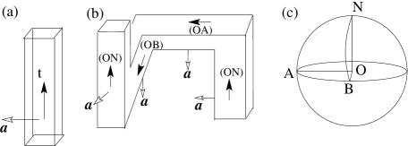
Figure 10: (a) A long bar of rectangular cross section. Unit vector ${\bf t}$ is along the axis, and ${\bf n}$ perpendicular to one side. (b) The bar is bent into a twisted form. The two vectors at intermediate positions are as shown. A change in the orientation of ${\bf n}$ by $\pi/2$ is visible as ${\bf t}$ returns to its original orientation. (c) $S^{2}$ as the space for vector ${\bf t}$. As one moves along the bar, ${\bf t}$ goes from ON to OA, OA to OB, and then back to ON, a closed path on $S^{2}$. The solid angle subtended by the closed region NABN is $\pi/2$. In the quantum mechanics problem, there is an extra factor of $1/2$ (see Eq. (40)).

Take a long bar of rectangular cross section so as to identify the sides easily. See Fig. 10. Define unit vectors ${\bf t}$ along the axis, and ${\bf a}$ perpendicular to one side. Orientations are to be kept fixed locally. The bar is bent into a twisted form as in Fig. 10b. The two vectors are monitored along the tube, keeping their orientations fixed locally. A $\pi/2$ change in the orientation of ${\bf a}$ is visible even when ${\bf t}$ gets back to its original orientation. To see this change, we note that vector ${\bf t}$, as a unit vector, spans a sphere $S^{2}$ as in Fig. 10c. As one moves along the bar, ${\bf t}$ goes from ON to OA, OA to OB, and then back to ON, a closed path on $S^{2}$. The solid angle subtended by the closed region NABN is $1/8$ of the sphere, i.e. $\pi/2$ which is the change in orientation of ${\bf n}$. One may straighten the bar in Fig. 10b to see that there is a twist though the axis may remain straight.

This is an example of a geometric phase, not necessarily topological, because the solid angle subtended by a closed loop depends on the details of the loop. The rotation of the Foucault pendulum as the earth rotates under it is another example of this geometric phase. This particular example and its generalizations are important in macromolecules like DNA and is called twist.

For a classical wave, polarized light, with ${\bf n}$ as the polarization direction and ${\bf t}$ as the direction of propagation, one may see a change in the direction of polarization. The angle appears as a phase there and is the classical analog of Berry’s phase. The classical phase is called the Pancharatnam phase. In classical dynamics, such an angle also occurs and is known as the Hannay Angle. For details on these see Ref. [7]

Analogous to this classical example, Berry’s phase is generally a geometrical phase, and in special situations, like the Aharonov-Bohm case, it becomes a topological phase. To repeat, a topological phase is independent of the details of the path (same for all homotopic loops) while a geometrical phase is, in general, dependent on the details of the loop.

7.7 Examples: Spin-$1/2$ and Quantum two level system

7.7.1 Spin-$1/2$ in a magnrtic field

A counterpart of the problem discussed in Sec. 7.6 is a spin $1/2$ in a magnetic field with a Hamiltonian $H=-{\bf d}.\sigma$, where $\sigma$ is the 3-d vector of the Pauli spin matrices (See Sec 4.4.3). For a given field ${\bf d}$, there are two eigenstates, $\pm|d|$ with eigenvectors parallel or antiparallel to the direction of ${\bf d}$. As a vector, the field of constant magnitude $|d|$ can be in any direction in 3-dimensions, ${\bf d}=|d|\;\;(\sin\theta\cos\;\phi,\sin\;\theta\sin\;\phi,\cos\;\theta)$ with $\theta,\phi$ as the usual polar angles, spanning a sphere. The relevant space for the field is $S^{2}$. Let us choose the eigenstate for energy $+|d|$, (compare with Eq. (3)),

$$|u\rangle=\left(\begin{array}[]{c}\sin\frac{\theta}{2}e^{-i\phi}\\ -\cos\frac{\theta}{2}\end{array}\right),$$ (37)

upto an arbitrary phase factor. This $|u\rangle$ is a spinor, but, is, otherwise, fixed by the direction of the field ${\bf d}$. If the magnetic field is now rotated, it forms a closed loop on the sphere. To get the phase acquired by the wavefunction as given by Eq. (27), embed the sphere in three dimensions to obtain

$${\bf A}=\langle u|i{\bf\nabla_{d}}|u\rangle=\frac{\sin^{2}\frac{\theta}{2}}{|d|\;\sin\theta}\hat{\phi}=\frac{1}{2}\;\frac{1-\cos\theta}{|d|\;\sin\theta}\hat{\phi},\ {\rm with}\ {\bf\Omega}={\bf\nabla}\times{\bf A}=-\frac{1}{2}\frac{{\bf d}}{|d|^{3}},$$ (39)

in the radial direction. The line integral may be converted to a surface integral with the help of Stokes’ theorem, by choosing the enclosed part of the sphere as the relevant surface. As the area vector is radial, we see

$$\gamma=\int{\bf\Omega}\cdot d{\bf s}=-\frac{1}{2}\int d\omega=-\frac{1}{2}\;\mho_{c},$$ (40)

$d\omega,$ being the angular part of the spherical integral and $\mho_{c}$ is the solid angle formed by the closed loop. The similarity with the classical case of Fig 10 is to be recognized, except for the factor of $1/2$ which is purely a quantum mechanical contribution. A solid angle is a geometrical quantity, dependent on the closed path, and so the phase here, unlike the Aharonov-Bohm phase, is not topological. The form of the “magnetic field” ${\bf B}$ shows that there is a singularity at $d=0$, the degeneracy point and the functional form of ${\bf\Omega}$ satisfies ${\bf\nabla}\cdot{\bf\Omega}=4\pi\;\delta({\bf r})$ with $g=-1/2$ and $\delta({\bf r})$ as the Dirac $\delta$-function. With ${\bf\Omega}$ as a “magnetic field”, it looks like there is a magnetic monopole $g=-1/2$ at the center, and the Berry phase is the flux due to this monopole through the loop.

The magnetic monopole interpretation helps us in identifying a topological invariant, using the equivalent of the Gauss theorem. An integration over the whole sphere is the flux through the closed surface and it counts the number of monopoles enclosed by the sphere. In other words

$$C_{1}\equiv\frac{1}{2\pi}\ \int_{S^{2}}{\bf\Omega}\cdot d{\bf s}=n\in\mathbb{Z}.$$ (41)

This is the first Chern number as defined in Eq. (33).

It is important to see from a different view point why $C_{1}\neq 0$. Let us divide the surface integral into parts at the equator. The closed loop integral $\oint{\bf A}\cdot d{\bf l}$ can be evaluated with the help of Stokes theorem with either the upper hemisphere containing the North pole or the lower hemisphere containing the South pole, provided ${\bf A}$ can be defined uniquely on the chosen surface and the equator. Since Eq. (37) is valid for the part of the sphere that encloses the North pole, we get, for the upper hemisphere (uh), $\oint{\bf A}\cdot d{\bf l}=\int_{\rm uh}d{\bf s}\cdot{\bf\Omega}$ which evaluates to $+\pi$. However, this choice of $|u\rangle$ cannot be used for the lower hemisphere (lh), as the spinor, Eq. (37), has undefined phase at the South pole ($\theta=\pi$) where $|u\rangle=(e^{i\phi}\ 0)^{T}\equiv(1\;\;0)^{T}$. A possible choice (“choice of gauge”) is $|u_{lh}\rangle=(\sin(\theta/2),-\cos(\theta/2)e^{i\phi})^{T}$ which is now defined everywhere on the sphere except the North pole ($\theta=0$). With this choice ${\bf A}=-\frac{1}{2}\;\frac{1+\cos\theta}{|d|\;\sin\theta}\hat{\phi}$, though the curvature ($\Omega$) remains the same as Eq. (39). A direct line integral over the equator ($\theta=\pi/2$) gives $-\pi=\pi-2\pi$. In other words it differs from the upper hemisphere result by $-2\pi$ which does not matter as an angle. If Stokes theorem is used, $\oint{\bf A}\cdot d{\bf l}=-\int_{lh}{\bf\Omega}\cdot d{\bf s}$ with a minus sign coming from the direction rule of the theorem. Since it is the same line integral, We must have $(\int_{uh}+\int_{lh}){\bf\Omega}\cdot d{\bf s}=0$ upto $2\pi n,n\in{\mathbb{Z}}$. In this particular case, we find $-2\pi$ whose origin lies in the nonuniformity of the guage choice. If a single gauge choice can be done over the whole surface, then the surface integral would have been zero. Thus the zero Chern number corresponds to the trivial case, while a nonzero Chern number tells us that more than one map is needed to cover the whole closed surface. In this case we need two.

For the $S^{2}$ case, the state is given by $-{\hat{n}}$ which is also the normal to the surface. The Berry curvature, Eq. (29) is given by

$$\Omega_{lm}=-\frac{1}{2}{\hat{n}}\cdot\left(\frac{\partial{\hat{n}}}{\partial R_{l}}\times\frac{\partial{\hat{n}}}{\partial R_{m}}\right),$$ (42)

where the derivatives are now the angular derivatives, and it is same as ${\bf B}$ in Eq. (39). The Chern number can therefore be written as

$$C_{1}=-\frac{1}{4\pi}\ \int_{S^{2}}\;ds\;\;{\hat{n}}\cdot\left(\frac{\partial{\hat{n}}}{\partial\theta}\times\frac{1}{\sin\theta}\frac{\partial{\hat{n}}}{\partial\phi}\right)=-1.$$ (43)

The analysis for Berry’s phase can be done for the other state $|v\rangle$ with eigenvalue $-|d|$. In that case the monopole will be of charge $+1/2$ so that the total of all the states is zero, consistent with Eq. (32).

7.7.2 Case of two bands: Chern insulators

The results of the two level system in the previous section finds a ready use in a two band system. This situation arises for a band insulator where we may focus on the last occupied band and the next unoccupied band.

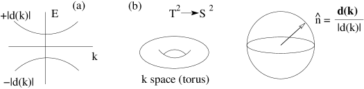
Figure 11: (a) Schematic diagram of two bands vs k. The band energies are $\pm|d({\bf k})|$. (b) In two dimensions the k-space is a torus ${\mathbb{T}}^{2}$ while unit vector ${\hat{n}}({\bf k})={\bf d}({\bf k})/|d({\bf k})|$ lies on a sphere. This gives a ${\mathbb{T}}^{2}\to S^{2}$ map.

The bands are described by the pseudomomentum ${\bf k}$ in the first Brillouin zone. The Hamiltonian can be written as $H=-{\bf d(k)}\cdot{\bf\sigma}$, with the bands given by $\pm|d({\bf k})|$. For a two dimensional problem, the $k$-space (or the first Brillouin zone) is a torus ${\mathbb{T}}^{2}$, while unit vector ${\hat{n}}({\bf k})={\bf d}({\bf k})/|d({\bf k})|$ maps out a sphere $S^{2}$. It may be visualized as a three component vector ${\bf n}$ attached to every point of the Brillouin zone torus. One may compare with the Heisenberg magnet example of Sec. 4.1, where we looked at the arrangements of three-vectors in Eucildean space. Here, instead of the Euclidean space, we now have a torus. All possible insulators can now be characterized by the “spin arrangements” on the torus. In the real space case of magnets, we found $\pi_{1}(S^{2})=0$, and so there is no topological distinction among the spin configurations in space. In the present case, the mapping is nontrivial, and that tells us that all insulators are not topologically equivalent. In other words, there are topologically inequivalent classes of insulators, identified by the arrangements of the gap vector ${\bf d}$ on the Brillouin Zone, which is a torus. The nontrivial ones are called topological insulators.

As we move along the torus, the ${\bf k}$-vector changes, and it acts as the parameter for Berry’s phase or equivalently the curvature. The topological invariant is then the first Chern number that tells us how many times (with sign) vector ${\hat{n}}$ goes around the sphere as one traverses the torus. This number comes from the Chern formula

$$C_{1}=\frac{1}{4\pi}\ \int\int d^{2}k\;\;{\hat{n}}\cdot\left(\frac{\partial{\hat{n}}}{\partial k_{x}}\times\frac{\partial{\hat{n}}}{\partial k_{y}}\right).$$ (44)

We have talked about the homotopy groups which allows one to explore a space by spheres $S^{n}$ for various integer $n$. But, instead of spheres, we may explore the space by tori as well. For the problem in hand, we are classifying the configurations of 3-component vectors on the torus. This is described by homotopy[${\mathbb{T}}^{2},S^{2}$] which is known to be ${\mathbb{Z}}$. The first Chern number is a concrete way of getting this integer for a particular case.

Let us choose an example,

$${\bf d}({\bf k})=(\sin k_{x},\sin k_{y},r+\cos k_{x}+\cos k_{y})).$$ (45)

If $|r|$ is very large, ${\hat{n}}$ is nearly along $(0,0,\pm 1)$, and so does not wind completely the sphere. The Chern number is zero as can be checked from Eq. (44) for $|r|>2$. One can easily check that $C_{1}=1$ if $-2<r<0$, while $C_{1}=-1$ if $0<r<2$. There is topology change but the change is not obvious from the band structure. The Chern number is not defined at $r=0,\pm 2$, the transition points. Exactly at $r=-2$, we see $|d|=0$ at $k_{x}=k_{y}=0$; this means the gap closes (no longer an insulator) at one point. For $r=2$, the gap closing occurs at $(\pi,\pi)$, while for $r=0$, it occurs at $(\pi,0)$ and $(0,\pi)$. The mapping to a sphere fails when a gap closes, and, consequently, a gap closing is important for a change of topology.

Band insulators with first Chern number=0 are called trivial insulators while those with $C_{1}\neq 0$ are called Chern insulators.[9].

Problem 7.1:

If the Hamiltonian for a two level system is real, i.e. $d_{y}=0$, show that Berry’s phase can be $0$ or $\pi$.

Problem 7.2:

General spin case: A spin-$J$ particle is in a magnetic field with Hamiltonian $H=-{\bf d}\cdot{\bf J}$. Consider any of the eigenstates, say, state $|J\;M_{J}\rangle$ which is an eigenstate of the Hamiltonian. Calulate the Berry phase when ${\bf d}$ rotates as in Sec. 7.7. It is easier to use Eq. (31). The answer is $-M_{J}\mho_{c}$, generalizing Eq. (40).

Problem 7.3:

Take the problem of a particle on a ring of radius 1, in presence of a magnetic flux threading the ring. This is the problem discussed above but there is now a potential $V(x)=v\delta(x)$ on the ring so that the Hamiltonian is

$$H=\frac{1}{2m}(p+\theta)^{2}+v\delta(x),$$ (46)

under periodic boundary condition $\psi(x)=\psi(x+2\pi)$. Use topological arguments and necessary gauge transformations to identify this problem as the Dirac comb problem (one dimensional Kronig Penny model). Use Bloch’s theorem to show that $\theta$ plays the role of the quasi-momentum.

Problem 7.4:

For a one dimensional model, the Brillouin zone is a circle. The two band problem then corresponds to a mapping $S^{1}\to S^{2}$. Discuss the nature of this mapping.

Discuss the general $d$-dimensional case, $T^{d}\to S^{2}$.

Problem 7.5:

Complete the calculations for the Berry phase, Berry curvature and the monopole, counterparts of Eqs. (39)- (43), for the eigenstate with eigenvalue $-|d|$.

Problem 7.6:

Take the example of Eq. (45) for three different values of $r$, $r=-1,1,3$. Draw the energy bands (3d plot) against $k_{x},k_{y}$. Separately, map out the region on a sphere traced out by ${\bf n}={\bf d}({\bf k})/|d({\bf k})|$ as ${\bf k}$ is taken over the Brillouin zone.

Problem 7.7:

The two bands in Sec. 7.7.2 are taken to have a special symmetry so that the midpoint of the gap is independent of ${\bf k}$. In general, the form of the Hamiltonian should be $H=-{\bf d(k)}\cdot{\bf\sigma}+d_{0}({\bf k}){\bf I}$, so that the space for the Hamiltonian is 4-dimensional. Show that the arguments of that section are not affected by $d_{0}({\bf k})$. In other words, it is justified to consider a 3-dimensional subspace.

Problem 7.8:

For the Aharonov-Bohm geometry, we saw the importance of winding around the hole. Consider the free particle case in a plane with a hole at origin. By a transformation $t=i\tau$ (imaginary time transformation), the Schrödinger equation can be converted to a diffusion equation which describes a Brownian particle in continuum. The winding of the Brownian particle around the hole can be measured by making the angle $\theta$ a real variable (refer to Fig. 1b,c). Show that for such a Brownian particle in a plane with a hole at origin, the probability distribution for winding angle $\theta(t)$ for large $t$ is

$$P(n)=\frac{1}{\pi}\;\frac{1}{1+x^{2}},\quad{\rm where}\;x=\frac{2\theta(t)}{\ln t}.\quad{\rm(Spitzer\ law)}$$ (47)

The infinite variance of this distribution is because of the large number of very small windings a particle can do around the hole.

8 DNA

A situation where the topology of two circles is needed is DNA. We saw the importance of two circles $S^{1}$ in Fig. 3. DNA involves a different type of topological problem.

Figure 12: DNA. (a) open DNA with $N$ base pairs. On melting it gives two separate strands. (b) A circular DNA on melting gives two separate rings. (c) If a $2\pi$ twist is given before forming the closed loop, then on melting there are again two nonpaired rings but now topologically linked. Helicity of the DNA is ignored here.

Double stranded DNA consists of two chains, called strands, connected together by base pairings. Suppose there are $N$ base pairs, making the strand length proportional to $N$. See Fig 12. In the completely bound state, the energy is $E=-N\epsilon$, where $-\epsilon$ is the hydrogen bond energy and $N$ is large. If the double stranded DNA has an entropy $s_{b}$ per base pair, then the bound state free energy is given by $F_{b}=-N\epsilon-TNs_{b}$ at temperature $T$. On the other hand if all the hydrogen bonds are broken, then there are two nonpaired separate chains, each with entropy $s_{0}$ per base. Since there is no energetic contribution, the free energy of the unbound state $F_{u}=-2NTs_{0}$. Evidently, the entropy per base of a single strand is higher than that of a double stranded DNA, and so a phase transition from the bound to the unbound state is possible at $T_{c}=\epsilon/(2s_{0}-s_{b})$. This is called the melting transition of a DNA. A real melting is a slightly more complicated phenomenon but this simple minded picture is sufficient here for our purpose. DNA strands can also be separated by force at $T<T_{c}$ and that is called unzipping transition.

DNA strands need to be separated because, as per semi-conservative replication, each of the new daughter molecules carry one of the original strands. DNA can be open or closed like a circular ring (or a ribbon). For example in many virus or bacteriophages, DNA is in an open state but after infection it closes to form a circular DNA. A circular DNA (with $N\to\infty$) will also undergo similar melting transition into two separate circular DNA as in Fig. 12b. It is possible that there are other events disrupting a smooth joining of the ends. Suppose there is a $2\pi$ twist of the ribbon before joining to form a twisted circular DNA (not a Möbius strip). This long DNA will also undergo a melting transition to give two nonbonded single stranded circles, but the two circles are linked topologically. From a thermodynamics ot statistical mechanical point of view, the slight change in the “boundary conditions” in the three cases shown in Fig. 12 do not matter but from a biological point of view, case (c) is dead or inactive because two the strands cannot be shared by the daughter virus or phages. We recognize the importance of topological constraints in biology though it does not affect the thermodynamical quantities like energy or entropy much.

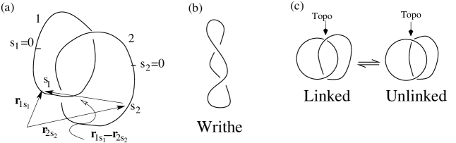
Figure 13: (a) Two loops with contour variables $k_{1}$ and $k_{2}$, and position vectors used in Eq. (48). (b)The coiling of the axis of the loop is called writhe. In DNA this leads to supercoiling. (c) Two linked DNA with TopoIV (Topoisomerase IV is a type of Topoisomerase II). TopoIV cuts both the starnds of a DNA, allows the other double stranded DNA to pass through the cut, and then rejoins the cut strands. Left to right: TopoIV unlinks the two DNA’s; right to left: two unlinked DNA’s get topologically linked.

8.1 Linking number

That cases (b) and (c) of Fig. 12 are different can be seen by studying a topological invariant called Gauss linking number. For simplicity we assume that each of the strand is free to cross itself (“phantom” chain) but they are mutually avoiding. In other words a chain cannot cross the other. This prevents the two circles becoming disentangled in case (c). If ${\bf r}_{is_{i}}$ denotes the position vector of the point of chain $i(i=1,2)$ at position $s_{i}$ measured along the chain from an arbitrarily chosen point $s_{i}=0$, then the Gauss linking number is given by[8]

$$Lk=\frac{1}{4\pi}\oint ds_{1}\oint ds_{2}\left[\left(\frac{\partial{\bf r}_{1s_{1}}}{\partial s_{1}}\right)\times\left(\frac{\partial{\bf r}_{2s_{2}}}{\partial s_{2}}\right)\right]\cdot\frac{{\bf r}_{1s_{1}}-{\bf r}_{2s_{2}}}{|{\bf r}_{1s_{1}}-{\bf r}_{2s_{2}}|^{3}},$$ (48)

where the integrals are from $s_{i}=0,N$, assuming both the chains to be of same length. $Lk$ is zero for cases (a) and (b), but nonzero for (c) for which it is 1. Since each chain can cross itself, one of the two, say 1, can be flattened into a planar circle. The linking number then counts the number of times chain 2 pierces loop 1. If we put a direction on each of the two strands in the direction of increasing $s_{1},s_{2}$ as if there are currents in the loops, then the counting rule can be proved by using Ampere’s law in magnetism (see problem). Because of the directions on the loops, $Lk$ can be positive or negative.

The two integrals over the closed loops of the contour variables $s_{1},s_{2}$, can be rewritten as a two dimensional integral over a torus, ${\bf k}=(s_{1},s_{2})$, as $S^{1}\times S^{1}={\mathbb{T}}^{2}$. If we define a unit vector

$${\hat{n}}({\bf k})=\frac{{\bf r}_{1s_{1}}-{\bf r}_{2s_{2}}}{|{\bf r}_{1s_{1}}-{\bf r}_{2s_{2}}|},$$

then the integral in Eq. (48) can be written as

$$Lk=\frac{1}{4\pi}\;\int\!\!\!\int_{\mathbb{T}^{2}}d^{2}k\;\;{\hat{n}}\cdot\left(\frac{\partial{\hat{n}}}{\partial s_{1}}\times\frac{\partial{\hat{n}}}{\partial s_{2}}\right),$$ (49)

which is identical in form as the Chern number integral for insulators, Eq. (44). Since ${\hat{n}}$ maps out a sphere, the linking number actually counts how many times ${\hat{n}}$ winds around the sphere as one covers the whole torus. This is the same number one looks for Chern insulators, but now the context is vastly different.

8.2 Twist and Writhe

As mentioned already, the linking number remains invariant under melting, which does not allow chain breaking. For the unbound phase, this is the only relevant topological invariant of interest, but for the bound phase there can be other geometrical quantities. Refer to Fig. 10. Consider a ribbon like object by making the cross-section very thin. The unit vector along the axis, ${\bf t}(s)$ represents the local DNA orientation in space, while ${\bf a}(s)$ is the hydrogen bond vector at contour position $s$ measured along the axis of the ribbon. With the third direction, we have a triad, a local coordinate system. The ribbon or the bar is closed so that at the end of the loop, ${\bf t}$ comes back to its original position (${\bf t}(0)={\bf t}(L)$, thereby forming a closed loop on $S^{2}$ as in Fig. 10c. The solid angle formed by the loop is the change in the orientation of ${\bf a}$. The twist can be defined by

$$Tw=\frac{1}{2\pi}\oint\;ds\;\;{\bf a}(s)\cdot\left(\frac{\partial{{\bf a}}}{\partial s}\times\frac{\partial{{\bf t}}}{\partial s}\right),$$ (50)

which need not be an integer. There is another geometric quantity that determines the twisting of the axis as in Fig. 13b. It is given by a formula similar to the linking number formula except that both the integrations are over the same loop formed by the axis,

$$Wr=\frac{1}{4\pi}\oint ds\oint ds^{\prime}\left[\left(\frac{\partial{\bf r}_{s}}{\partial s}\right)\times\left(\frac{\partial{\bf r}_{s^{\prime}}}{\partial s^{\prime}}\right)\right]\cdot\frac{{\bf r}_{s}-{\bf r}_{s}}{|{\bf r}_{s}-{\bf r}_{s^{\prime}}|^{3}}.$$ (51)

Note that $s=s^{\prime}$ does not pose a problem because the crossproduct is also zero. $Wr$ is a continuous variable and can be changed by deforming the loop. It depends only on the shape but not on the scale. The sign of $Wr$ tells us the overall handedness of the coil – right or left handed. An important theorem by Călugăreanu connects the topological invariant $Lk$ to the two geometrical quantities as

$$Lk=Tw+Wr.$$ (52)

If we now consider the ensemble of all possible closed configurations of the double stranded DNA, with the relaxed state (energetically minimum state) with zero twist and zero writhe, we have $\langle Lk\rangle=\langle Tw\rangle=\langle Wr\rangle=0$. Intuitively, twist and writhe are independent. Therefore, the variances are additive, $\langle Lk^{2}\rangle=\langle Tw^{2}\rangle+\langle Wr^{2}\rangle$. For a real DNA of length $L$ with a helical pitch of $\gamma$, the normal relaxed state will have $Tw_{0}=L/\gamma$ In that case the averages satisfy $\langle Tw-Tw_{0}\rangle=\langle Wr\rangle=0$, and $\langle(\Delta Lk)^{2}\rangle=\langle(\Delta Tw)^{2}\rangle+\langle(\Delta Wr)^{2}\rangle$ where $\Delta$ denotes deviation from the average. The variances of $Tw,Wr$ can be related to the elastic constants of the DNA, allowing us to link topological or geometrical features to the elastic constants. Although, $Lk$ remains constant at melting but $Tw,Wr$ lose their meaning in the unbound phase, or even in partially unzipped state.

8.3 Problem of Topoisomerase

Biological processes require trivial $L$. Two closed loops with different $L$ cannot be deformed into one another and therefore belong to topologically different classes. Note that this is true only in three dimensions (${\bf r}$’s are 3-dimensional vectors). An example is shown in Appendix B on opening up this link in four dimensions without any cut-paste.

There are enzymes called Topoisomerase II (topoisomerase IV to be precise) that can cut a double stranded DNA at a crossing, change the value of $Lk$ as shown in Fig. 13c, and rejoin the cut DNA. This is needed in biology to separate two circular DNAs after replication. What is surprising is that the topoisomerase can locally do a cut-paste to make the change. In the figure only minimal number of crossings are shown. There could be many trivial crossings. As the topological feature is a global one (the integrations over the two loops are equivalent to scanning the whole chains), how an object, acting locally, can achieve this is a big puzzle. It is easy to see that, in thermal equilibrium, any crossing changed at random can produce a link as often as it may open it up. One wonders if Topoisomerase knows of the fourth dimension!

Problem 8.1:

Show the equality of the two expressions in Eqs. (49) and (48).

Problem 8.2:

Use the standard formula of magnetic field $d{\bf B}({\bf r})$ at ${\bf r}$ due to a small current element $d{\bf l}$ at ${\bf r}^{\prime}(l)$, $d{\bf B}({\bf r})\propto d{\bf l}\times{\bf\nabla}\frac{1}{|{\bf r}-{\bf r}^{\prime}(l)|}$ and Stokes’ theorem to prove that $Lk$ in Eq. (48) is an integer..

Problem 8.3:

Show that $Tw$ is additive, i.e. it can be computed by adding twists for pieces. Show that writhe is zero for a planar figure.

Problem 8.4:

Prove Călugăreanu’s theorem.

Problem 8.5:

Show that for a double starnded DNA loop, Topoisomerase IV changes writhe by $\pm 2$.

9 Summary

In this chapter we explored several simple problems from classical mechanics, statistical mechanics, and quantum mechanics by using topological arguments. These, in turn, allowed us to explain some of the basic ideas of elementary topology in terms of the known physical phenomena, and the common link among diverse topics.

Appendix A: Mobius strip and Stokes’ theorem

Let us now discuss a different type of problems involving integrals of vector fields. Stokes’ theorem states that the surface integral of the curl of a vector field is equal to the line integral of the field over the boundary of the surface.

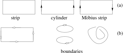
Figure 14: Cylinder, Möbius strip and Stoke’s law.

Take a rectangular strip (say, a long piece of paper) of length $2\pi{{R}}$ and width $2L$ as in Fig. 14a. Now use the arrows to define “equivalence” condition, namely periodic boundary condition in the x-direction to get a cylinder and with a twisted boundary condition (“half-twist”) to get a Möbius strip. These two in 3 dimensions can be described by

$${\rm cylinder:} x(t,\theta)=R\cos\theta,y(t,\theta)=R\sin\theta,z(t,\theta)=t,$$ (53)

$${\rm Mobius:} x(t,\theta)=\left(R-t\sin\frac{\theta}{2}\right)\cos\theta,y(t,\theta)=\left(R-t\sin\frac{\theta}{2}\right)\sin\theta,$$ (54)

$$z(t,\theta)=t\cos\theta,$$

for $-L\leq t\leq L$ and $0\leq\theta<2\pi$.

The cylinder has two boundaries at $t=-L$ and $t=L$, but the Möbius strip has only one boundary. For the Möbius strip, we reach the same point by going around twice, so that the boundary can be described by Eq. (54) with $t=L$ and $0\leq\theta\leq 4\pi$. It actually consists of the two original boundaries at $t=L,0\leq\theta\leq 2\pi$ and $t=-L,0\leq\theta\leq 2\pi$ joined together to form an unknot, as can be seen in Fig. 14b.

Suppose we have a vector field

$${\bf A}=\hat{k}\times\frac{{\vec{\rho}}}{\rho^{2}},$$

where $\vec{\rho}=x\hat{\imath}+y\hat{\jmath}$ in the same three dimensional coordinate system. For this field $\nabla\times{\bf A}=0$ everywhere except for the z-axis.

We now consider the three geometries of Fig. 14a separately.

1. Let us now put the strip in Fig. 14 say parallel to the z axis with the centre at $(R,0,0)$. The surface integral $\int\!\int d{\vec{S}}\cdot(\nabla\times{\bf A})=0$. It is easy to check that Stokes’ theorem is valid by showing that the line integral $\oint{\bf A}\cdot d{\bf l}=0$, where the integration is along the boundary, as shown in the left figure of Fig. 14b.

2. For the cylinder placed along the z-axis with the centre of the cylinder at the origin, there are two boundaries along which one has to do the line integral. Since the directions are opposite for the two rings at $z=\pm L$ (middle fig of Fig. 14b), the total line integral is zero. In other words Stokes’ theorem is explicitly verified.

3. For the Möbius case, the line integral along the boundary curve is

   $$\oint_{\rm boundary}{\bf A}\cdot d{\bf r}=\int_{0}^{4\pi}{\bf A}(x(\theta),y(\theta),z(\theta))\cdot{\bf r}^{\prime}\ {d\theta}\neq 0,$$

   where ${\bf r}^{\prime}=d{\bf r}/d\theta$. For the parametrization used, ${\bf A}\cdot{\bf r}^{\prime}=1$ so that the integral is $4\pi$. There seems to be a violation of Stokes’ law.

This paradox is resolved by noting that the area vector $d{\bf S}$ cannot be defined on the Möbius strip. If we slide a small area element along the strip through $2\pi$ the area vector will not point in the same direction. Another way of seeing the difference is to colour the surfaces without any abrupt change. Two colours are needed to paint the surfaces of the strp and the cylinder, but one is enough for the Möbius strip. Such a surface, like the Möbius strip, is called a nonorientable surface and Stokes’ theorem is not applicable there.

Problem 9.1:

Is it possible to generalize the Möbius strip construction so that the boundary curve is, say, a trefoil knot? (Hint: three half-twists)

Appendix B: Disentanglement via moves in 4-dimensions

Take two loops with linking number one. It is a common knowledge that the two loops cannot be taken apart if the chains do not cross each other. We now show a set of local moves in four dimensions (x-y-z-w space) that takes (b) to (c) in Fig. 15.

Figure 15: (a) Linked loops. The crossing indicted by the dotted circle is shown in (b). In three dimensions, chain 1 in (b) is in the plane $z=-1$ while the other one is at $z=0$ so that chain 1 is below chain 2. The crossing point is taken to be at $x=y=0$ when projected in the xy plane. If the chain configurations can be changed to type (c), then the two loops can be unlinked. This is possible in 4-dimensions but not in three.

Let $t$ be a parameter, $t\in[0,1]$, so that chain 1 can be parameterized in 4-dimensions by

$$f_{0}(t)=\left\{\begin{array}[]{ll}(-a,-a,-{1},0)&\quad(0\leq t\leq\frac{3}{8})\\[5.0pt] (-a+8a(t-\frac{1}{8}),-a+8a(t-\frac{1}{8}),-1,0)&\quad(\frac{3}{8}\leq t\leq\frac{5}{8})\\[5.0pt] (a,a,-1,0)&\quad(\frac{5}{8}\leq t\leq 1)\end{array}\right.$$ (58)

We shall deform the chain in three mutually exclusive ways, (i) in the xy plane, or, (ii) in the z-direction, or, (iii) in the 4th w direction. The variable $t$ is used to describe the configuration of the chain, while a second variable $s\in[0,1]$ is to be used for the deformation so that the chain is described as $f_{s}(t)$.

First we deform in the x-y-w space keeping $z=-1$ fixed. The new chain at $s=1/3$ is given by

$$f_{1/3}(t)=\left\{\begin{array}[]{ll}(-a,-a,-1,8t),&\quad(0\leq t\leq\frac{1}{8})\\[5.0pt] (-a,-a,-1,1),&\quad(\frac{1}{8}\leq t\leq\frac{3}{8})\\[5.0pt] (-a+8a(t-\frac{3}{8}),-a+8a(t-\frac{3}{8}),-{1},1),&\quad(\frac{3}{8}\leq t\leq\frac{5}{8})\\[5.0pt] (a,a,-1,1),&\quad(\frac{5}{8}\leq t\leq\frac{7}{8})\\[5.0pt] (a,a,-1,1-8(t-\frac{7}{8})),&\quad(\frac{7}{8}\leq t\leq 1)\end{array}\right.$$ (64)

Next, we deform the $z$ coordinate from -1 to 1 taking the chain above the other one as

$$f_{2/3}(t)=\left\{\begin{array}[]{ll}(-a,-a,-1,8t),&\quad(0\leq t\leq\frac{1}{8})\\[5.0pt] (-a,-a,-1+16(t-\frac{1}{8}),1),&\quad(\frac{1}{8}\leq t\leq\frac{2}{8})\\[5.0pt] (-a,-a,1,1),&\quad(\frac{2}{8}\leq t\leq\frac{3}{8})\\[5.0pt] (-a+8a(t-\frac{3}{8}),-a+8a(t-\frac{3}{8}),{1},1),&\quad(\frac{3}{8}\leq t\leq\frac{5}{8})\\[5.0pt] (a,a,1,1),&\quad(\frac{5}{8}\leq t\leq\frac{6}{8})\\[6.0pt] (a,a,1-16(t-\frac{6}{8}),1),&\quad(\frac{5}{8}\leq t\leq\frac{7}{8})\\[6.0pt] (a,a,-1,1-8(t-\frac{7}{8})),&\quad(\frac{7}{8}\leq t\leq 1)\end{array}\right.$$ (72)

Finally, we bring back the fourth $w$ coordinate to zero as,

$$f_{1}(t)=\left\{\begin{array}[]{ll}(-a,-a,-1,0),&\quad(0\leq t\leq\frac{1}{8})\\[5.0pt] (-a,-a,-1+16(t-\frac{1}{8}),0),&\quad(\frac{1}{8}\leq t\leq\frac{2}{8})\\[5.0pt] (-a,-a,1,0),&\quad(\frac{2}{8}\leq t\leq\frac{3}{8})\\[5.0pt] (-a+8a(t-\frac{3}{8}),-a+8a(t-\frac{3}{8}),{1},0),&\quad(\frac{3}{8}\leq t\leq\frac{5}{8})\\[5.0pt] (a,a,1,0),&\quad(\frac{5}{8}\leq t\leq\frac{6}{8})\\[6.0pt] (a,a,1-16(t-\frac{6}{8}),0),&\quad(\frac{5}{8}\leq t\leq\frac{7}{8})\\[6.0pt] (a,a,-1,0),&\quad(\frac{7}{8}\leq t\leq 1)\end{array}\right.$$ (80)

It is now straight forward to construct a map $f_{s}(t)$ linear and continuous in $s$ – it is already linear and continuous in $t$ – that goes from $f_{0}(t)\to f_{1/3}(t)\to f_{2/3}(t)\to f_{1}(t)$. For example, for $2/3\leq s\leq 1$ a continuous map from $f_{2/3}(t)$ to $f_{1}(t)$ can be constructed by replacing the $w$ values of $f_{2/3}$ by $3w(1-s)$. Note that we get back the same boundary points $(-a,-a,-1,0)$ at $t=0$ and $(a,a,-1,0)$ at $t=1$ for all $s\in[2/3,1]$.

The two loops can therefore be delinked via these local deformations in the 4th dimension.

References

- [1] M. Nakahara, Geometry, Topology and Physics (Taylor & Francis, Boca Raton, FL, USA, 2003).
- [2] R. Aldrovandi and J. G. Pereira, An Introduction to Geometrical Physics (World Scientific, SIngapore, 1995).
- [3] C. Nash, S. Sen, Topology and Geometry for Physicists (Dover, Mineola, NY, 2011).
- [4] See, e.g., the chapters by Somnath Basu, and by Atreyee Bhattacharya in this book.
- [5] See, e.g., the chapters by Samik Basu, and the tutorial by Soma Maity in this book.
- [6] See, e.g., the chapter by Dheeraj Kulkarni in this book.
- [7] Geometric Phases in Physics, Edited by: F Wilczek and A Shapere (World Scientific, Singapore, 1989)
- [8] See, e.g., the chapters by Mahan Mj, and by P. Ramadevi in this book.
- [9] For an example of an insulator with Chern number=2, see P. Titum, N. H. Lindner, M. C. Rechtsman, and G. Refael, Phys. Rev. Lett. 114, 056801 (2015).