Photon-assisted shot noise in graphene in the Terahertz range

Abstract

When subjected to electromagnetic radiation, the fluctuation of the electronic current across a quantum conductor increases. This additional noise, called photon-assisted shot noise, arises from the generation and subsequent partition of electron-hole pairs in the conductor. The physics of photon-assisted shot noise has been thoroughly investigated at microwave frequencies up to 20 GHz, and its robustness suggests that it could be extended to the Terahertz (THz) range. Here, we present measurements of the quantum shot noise generated in a graphene nanoribbon subjected to a THz radiation. Our results show signatures of photon-assisted shot noise, further demonstrating that hallmark time-dependant quantum transport phenomena can be transposed to the THz range.

The many promises of the Terahertz (THz) frequency range, in terms of both fundamental and practical applications, has led to the increasingly active development of various THz sources and detectors Ferguson2002 ; Tonouchi2007 ; Rogalski2011 . This recently allowed the study of fundamental aspects of time-dependent electronic quantum transport at higher frequencies, comparable with the characteristic energy scales arising in highly confined electronic systems, such as carbon nanotubes, self-assembled semiconductor quantum dots, and single molecule transistors Kawano2008 ; Shibata2012 ; Yoshida2015 . These previous works focused on photon-assisted tunnelling (PAT), wherein electron transport across a discrete electronic level is mediated by the absorption of a resonant impinging photon Tien1963 ; Tucker1985 ; Kouwenhoven1994 . The ability to reliably couple THz-range radiation to electronic transport degrees of freedom in a quantum conductor significantly broadens the range of exploration of the influence of electron-photon interactions on charge transport. These interactions, which have been extensively studied in the microwave range, can give rise to striking modifications of the conductance of a coherent conductor, by either increasing it, as it is the case for PAT, or strongly suppressing it in the so-called dynamical Coulomb blockade Nazarov1992 .

Electron-photon interactions can have subtle effects, which do not appear in the electronic conductance, but rather in the fluctuations of the current across the quantum conductor, or quantum shot noise. Such is the case for photon-assisted shot noise (PASN), a hallmark of time-dependent electronic quantum transport where incident photons excite electron-hole pairs in the leads of a coherent conductor Lesovik1994 ; Blanter2000 ; Schoelkopf1998 ; Kozhevnikov2000 ; Reydellet2003 ; Gasse2013a ; Gabelli2013 ; Dubois2013 ; Jompol2015 . The electron-hole pairs then propagate in the conductor, in which quantum partitioning leads to an increase of shot noise, while the net current remains zero. This increase can be expressed as an equivalent noise temperature $T_{N}$:

$$T_{N}=T_{el}+F\sum_{n}J_{n}^{2}(\frac{eV_{\mathrm{ac}}}{h\nu})\\ \times\frac{eV_{\mathrm{dc}}+nh\nu}{2k_{B}}\left[\mathrm{coth}\left(\frac{eV_{\mathrm{dc}}+nh\nu}{2k_{B}T_{el}}\right)-\frac{2k_{B}T_{el}}{eV_{\mathrm{dc}}+nh\nu}\right],$$ (1)

where $V_{\mathrm{dc}}$ is the dc drain-source voltage applied to the conductor, $V_{ac}$ and $\nu$ are the amplitude and frequency of the electromagnetic radiation, $T_{el}$ is the electron temperature, $F$ is the Fano factor characterizing transport in the conductor, $J_{n}$ are Bessel functions of the first kind, $e$, $h$ and $k_{B}$ are respectively the electron charge, Planck’s and Boltzmann constants. Predicted more than two decades ago Lesovik1994 , and extensively studied in the microwave domain Schoelkopf1998 ; Kozhevnikov2000 ; Reydellet2003 ; Gasse2013a ; Gabelli2013 ; Dubois2013 ; Jompol2015 , PASN remarkably allows reconstructing the out-of equilibrium energy distribution function arising in the conductor due to the time-dependent potential Gabelli2013 ; Dubois2013 , as well as calibrating the amplitude and frequency of a monochromatic radiation impinging on the conductor Gasse2013a .

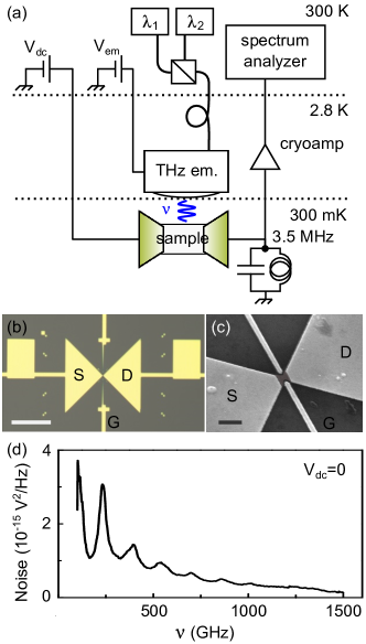
Figure 1: (a), Simplified schematic description of our setup combining a photomixing THz source and noise measurements. The THz emitter (thermally anchored to the 2.8 K stage of the refrigerator) is aligned in front of the sample (set at 300 mK), the shot noise of which is measured through a resonant LC circuit. (b), Optical micrograph of a typical sample, showing the bow-tie antenna-shaped electrodes (S and D). The scale bar corresponds to 50 $\mu$m. (c), Scanning electron micrograph of a typical sample, showing the tip of the electrodes, as well as the side gate (G). The shape of the graphene ribbon is shown in light grey. The scale bar corresponds to 1 $\mu$m. (d), Integrated excess noise power at the output of the setup as a function of the frequency of the THz radiation, measured on sample A.

To unveil the signatures of PASN due to THz radiation, we have measured the shot noise of graphene coherent conductors in presence of a THz excitation. Graphene, which has been shown to host a variety of striking linear and nonlinear optical effects, such as wide-spectrum saturable absorption Bonaccorso2010 , is particularly well suited for THz applications, its high mobility Mayorov2011 and low electron-phonon coupling Balandin2011 allowing its use in a large number of THz detectors based on different mechanisms Koppens2014 . We rely on the ability to easily engineer ribbons of disordered graphene, in which electronic transport is diffusive Chen2009 . Using a diffusive conductor has several advantages for the noise measurements presented here. First, the sample conductance is essentially independent of the energy up to high energies. This ensures that, in absence of THz excitation, the shot noise is indeed linear with the drain-source voltage $V_{\mathrm{dc}}$, and devoid of features which would mask the signatures of PASN. This also allows neglecting the effects of photon-assisted tunnelling (which only occurs in energy-dependent conductors), which would generate an additional shot noise with strong dependences in $V_{\mathrm{dc}}$, again potentially masking the signatures of PASN. Second, the value of the Fano factor $F=1/3$ is well known for diffusive conductors Blanter2000 , simplifying the analysis.

Fig. 1(a) shows a simplified description of our experimental setup SM . We use a Toptica cw THz generator based on a photomixing technique Deninger2008 ; Roggenbuck2010 to illuminate the samples in the 50 GHz - 2 THz range. The emitter, consisting of a rapid photo-switch coupled to a focusing Silicon lens, is aligned in vacuum a few mm above the sample, which is cooled down to 300 mK. The (uncalibrated) power of the THz radiation is modulated by the bias voltage $V_{\mathrm{em}}$ applied to the diode. Fig. 1(b) and 1(c) show optical and scanning electron micrographs of a typical sample, consisting of a CVD grown monolayer graphene nanoribbon connected to source and drain electrodes shaped as the two parts of a bow-tie antenna. Side gates (labelled $G$) allows tuning the transport through the nanoribbon. A dc voltage $V_{\mathrm{dc}}$ is applied across the sample, and the power spectral density of the shot noise it generates is filtered through an LC tank with a resonance frequency $f_{\mathrm{LC}}\approx 3.5$ MHz, and a bandwidth at half maximum $\Delta f_{\mathrm{LC}}\approx 0.4$ MHz. This is crucial to increase the sensitivity and stability of the measurement, as $1/f$ noise and microphonics are absent in this frequency range Dicarlo2006 . The noise signal is then amplified using home-made cryogenic amplifiers (input voltage noise $S_{\mathrm{V,}amp}\approx 0.14\leavevmode\nobreak\ \mathrm{nV}/\sqrt{\mathrm{Hz}}$). Fig. 1(d) shows the uncalibrated noise signal at the end of our detection chain as a function of the frequency $\nu$ of the THz radiation at maximum power ($V_{\mathrm{em}}=13$ V), for a first sample (labelled A) at $V_{\mathrm{dc}}=0$. Clear oscillations appear as $\nu$ is swept; however, the precise frequency dependence of the signal is challenging to analyze, as it is not reproducible from sample to sample SM , and contains contributions of the emitter power frequency dependence (which is monotonously decreasing, with about -40 dB$/$decade Deninger2008 ; Roggenbuck2010 ), standing waves between the emitter and the samples, and of the frequency response of the sample’s antennas. A simple numerical simulation of the frequency response of the antenna showed resonances qualitatively similar to Fig. 1(d) SM . This nonetheless confirms that noise measurements in graphene and other nano-devices can be used for THz detection Santavicca2010 ; Wang2014 .

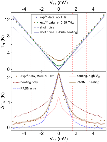
Figure 2: Upper panel: excess noise temperature $T_{N}$ as a function of the dc bias applied to the sample (sample B). The purple, green and brown symbols are the experimental data, respectively in absence of THz radiation ($V_{\mathrm{em}}=0$ V), at $\nu=0.39$ THz and $V_{\mathrm{em}}=10$ V, and at $\nu=0.39$ THz and $V_{\mathrm{em}}=13$ V. The dashed line is the expected shot noise in absence of heating, and the continuous line is a fit of the data without THz radiation, including heating. Lower panel: difference $\Delta T_{N}$ of the noise in presence ($V_{\mathrm{em}}=13$ V) and in absence of THz radiation. The red and blue dashed lines are fits of the experimental data using, respectively, a heating model and a PASN model. The thin continuous line is a fit of the data at large $V_{\mathrm{dc}}$ using a heating model, and the thick line is a fit combining this last model and a PASN model at low $V_{\mathrm{dc}}$. In both panels, the symbols size corresponds to the statistical error on the measurement. The red vertical dashed lines in both panels correspond to $eV_{\mathrm{dc}}=\left\{-2,-1,1,2\right\}h\nu$.

We now analyze the origin of the noise increase by measuring its dependence with $V_{\mathrm{dc}}$ in a second sample, labelled B. The upper panel of Fig. 2 shows the measured variations of the calibrated noise temperature $T_{N}=S_{i}/4k_{B}G_{s}$ with $V_{\mathrm{dc}}$, where $S_{i}$ is the current noise generated in the sample and $G_{s}$ is the conductance of the sample, measured simultaneously using standard lock-in techniques SM . We first show that in absence of THz radiation ($V_{\mathrm{em}}=0$, purple symbols), significant heating effects arise due to Joule power dissipated in the leads: the dashed line in the upper panel of Fig. 2, corresponding to shot noise with the Fano factor $F=1/3$ of diffusive coherent conductors and no heating, is markedly lower than the data. Importantly, the linear variation of $T_{N}$ with $V_{\mathrm{dc}}$ implies that cooling is only mediated by the electronic transport channels via the Wiedemann-Franz law, where the cooling power is proportional to the temperature $T_{el}$ squared SM . Indeed, if cooling mediated by electron-phonon coupling were important in the system, the noise would present sub-linear features, the cooling power due to electron-phonon coupling in graphene being proportional to $T_{el}^{\delta}$, with $\delta$ typically equal to 4 Betz2012a . A model using only the Wiedemann-Franz law yields the continuous line, in excellent agreement with the data. The ratio between the resistance of the graphene nanoribbon and the contact resistance is used as the fit parameter SM ; Kumar1996 . When the THz radiation at $\nu=0.39$ THz is turned on (green and brown symbols, for an emitter voltage $V_{\mathrm{em}}$ of resp. 10 V and 13 V), the noise clearly increases at low $V_{\mathrm{dc}}$, then approaches the data without THz radiation at $\left|V_{\mathrm{dc}}\right|>2$ mV. The increase at low $V_{\mathrm{dc}}$ is directly related to the voltage $V_{\mathrm{em}}$, and thus to the power of the THz radiation. The effect of the radiation appears more clearly when plotting the difference $\Delta T_{N}$ between the noise in presence and in absence of radiation, as shown in the lower panel of Fig. 2, for $\nu=0.39$ THz and $V_{\mathrm{em}}=13$ V. In particular, $\Delta T_{N}$ sharply decreases as $\left|V_{\mathrm{dc}}\right|$ increases on a typical energy scale given by $e\left|V_{\mathrm{dc}}\right|=h\nu$ (red dashed vertical lines), then saturates to a finite value at large $\left|V_{\mathrm{dc}}\right|$. This behaviour cannot be quantitatively reproduced by models describing the effect of THz as either pure PASN, or simple heating. Since the THz power impinging on the sample is not known by construction of the experiment, we use it (either as an ac amplitude $V_{\mathrm{ac}}$, or a temperature increase $T_{\mathrm{THz}}$) as the fit parameter in these models. In the first model (corresponding to the blue dashed line in the lower panel of Fig. 2), the noise is given by the PASN described in Eq. 1, where $\alpha=eV_{\mathrm{ac}}/h\nu$ is adjusted to fit the data at $V_{\mathrm{dc}}=0$, yielding $\alpha=1.3$, and the electronic temperature $T_{el}(V_{\mathrm{dc}})$ is extracted from the fit of the shot noise in absence of THz. Notably, the predicted $\Delta T_{N}$ is zero for $\left|eV_{\mathrm{dc}}\right|>2h\nu$, as PASN reduces to the usual shot noise when $V_{\mathrm{dc}}\gg V_{\mathrm{ac}}$, whereas the experimental data remains finite. In the second model (red dashed line), the noise is given by the usual shot noise expression (i.e. without ac excitation) Blanter2000 , where the electronic temperature is increased by a constant amount $T_{\mathrm{THz}}$, adjusted to fit the data at $V_{\mathrm{dc}}=0$: $T_{el}^{\ast}(V_{\mathrm{dc}})=\sqrt{T_{el}(V_{\mathrm{dc}})^{2}+T_{\mathrm{THz}}^{2}}$, with $T_{\mathrm{THz}}=2.41$ K. This dependence again stems from the fact that only electronic channels contribute to heat transport in the sample. Because of this dependence, the predicted noise decreases more slowly than the predicted PASN, or indeed, our experimental data. Note that 1) the statistical error on our data is much smaller than the difference between our data and either model, and that 2) regardless of the fitting procedure (adjusting the large $\left|V_{\mathrm{dc}}\right|$ value of the noise, or the entire curve), neither model allow to accurately describe our data. Since the experimental data clearly sits in between the results of both models, particularly at large $\left|V_{\mathrm{dc}}\right|$, we interpret it using a model combining both heating and PASN. We first extract $T_{\mathrm{THz}}=1.45$ K using the heating model to fit the data at large $V_{\mathrm{dc}}$ (thin continuous line), where the PASN theory predicts zero excess noise, then insert the increased temperature in the PASN formula while adjusting $\alpha=0.89$ to match the data at $V_{\mathrm{dc}}=0$. The result of this model, shown as a thick continuous line, is in excellent agreement with the data, over the whole range of explored $V_{\mathrm{dc}}$.

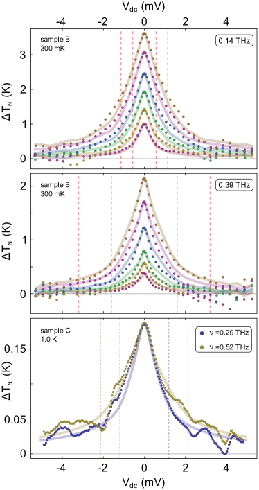
Figure 3: Top and central panels: noise difference $\Delta T_{N}$ for $\nu=$0.14 and 0.39 THz, measured at 300 mK on sample B. In both, $V_{\mathrm{em}}$ is changed from 8 (dark purple) to 13 V (dark yellow). Bottom panel: $\Delta T_{N}$ measured at 1 K on sample C for $\nu=$0.29 (blue) and 0.52 THz (dark yellow) and $V_{\mathrm{em}}=$13 V. In all panels, symbols are the experimental data, and continuous lines are fits combining heating and PASN, as explained in Fig. 2.

Fig. 3 shows the application of this analysis on experimental data obtained for various THz frequencies ($\nu$ ranging from 0.14 to 0.52 THz) and powers ($V_{\mathrm{em}}$ ranging from 8 to 13 V), and two different samples (sample B and C, respectively measured at 300 mK and 1 K). The excellent general agreement confirms the validity of our interpretation. While hot-electron effects smear the structures at $eV_{\mathrm{dc}}=h\nu$ expected from the PASN theory, the influence of the THz frequency on the noise can be seen as a broadening of the noise difference $\Delta T_{N}$ as a function of $V_{\mathrm{dc}}$ as $\nu$ increases, as shown in the lower panel of Fig. 3.

To emphasize the effect of $\nu$, we plot the maximum amplitude of the noise difference $\Delta T_{N}$, obtained at $V_{\mathrm{dc}}=0$, as a function of the corresponding values of $\alpha$ extracted from the fits shown in Fig. 3. The result is displayed in Fig. 4: the effect of $\nu$ appears clearly as a deviation from a linear behavior, more pronounced at high frequency. This deviation is well reproduced by a PASN model including heating caused by the THz radiation, shown as continuous lines. In contrast, a time-averaging model, where the noise is given by the average of usual shot noise under a periodic potential, yields a linear variation (dashed lines) Reydellet2003 .

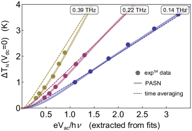
Figure 4: Noise difference $\Delta T_{N}$ at $V_{\mathrm{dc}}=0$ measured on sample B for $\nu=$0.14, 0.22 and 0.39 THz, as a function of $\alpha=eV_{\mathrm{ac}}/h\nu$ extracted from the fits explained in Fig. 2. The continuous lines are predictions of the model combining PASN and heating, and the dashed lines are predictions of the model combining heating and time-averaging of the shot noise. The size of the symbols indicates the uncertainty on the extraction of $\alpha$.

We finally analyze the performances of our system as a THz detector. Our data show that despite the low coupling to the emitter, we are able to apply ac voltages across the sample up to 2 mV in the hundreds of GHz range. We also extract the Noise Equivalent Power (NEP), defined as the power detected in a 0.5 s measurement with a signal-to-noise ratio of 1. Our setup allows detecting a typical variation in the noise $\delta T_{N}\left[SNR=1,t_{meas}=0.5\leavevmode\nobreak\ \mathrm{s}\right]\approx 14$ mK. At $V_{\mathrm{dc}}=0$, this corresponds to values of $\alpha$ between $0.05$ and $0.1$ in the PASN model including heating. When defining the radiation power $P_{\mathrm{ac}}=V_{\mathrm{ac}}^{2}/(2Z_{rad})$, where $Z_{rad}=376\leavevmode\nobreak\ \Omega$ is the vacuum impedance, we obtain a typical NEP smaller than $10\leavevmode\nobreak\ \mathrm{pW}/\sqrt{\mathrm{Hz}}$. While this value is comparable to the sensitivity of other THz detectors Rogalski2011 , it can be largely improved by adapting the sample impedance, and using an optimized microwave-frequencies noise measurement setup Parmentier2011 . Note also that heating effects tend to increase the sensitivity (as the noise signal is increased) at the cost of frequency discrimination, as the cusps in the noise at $eV_{\mathrm{dc}}=h\nu$ characteristic of PASN become smeared.

In summary, we have observed signatures of PASN in mesoscopic diffusive graphene ribbons, and shown that hallmark out-of-equilibrium phenomena of electronic quantum transport can be extended to energies much larger than the usually probed microwave domain. This allows envisioning fundamental physics experiments where the transport degrees of freedom of a coherent conductor are coupled to the energy spectrum of complex systems, e. g. molecules Ferguson2002 , as well as the development of new universal THz detectors based on PASN.

See pages 1 of parmentier-supplement-reresubmit.pdf See pages 2 of parmentier-supplement-reresubmit.pdf See pages 3 of parmentier-supplement-reresubmit.pdf See pages 4 of parmentier-supplement-reresubmit.pdf See pages 5 of parmentier-supplement-reresubmit.pdf See pages 6 of parmentier-supplement-reresubmit.pdf See pages 7 of parmentier-supplement-reresubmit.pdf See pages 8 of parmentier-supplement-reresubmit.pdf