High-dimensional simultaneous inference with the bootstrap

Abstract

We propose a residual and wild bootstrap methodology for individual and simultaneous inference in high-dimensional linear models with possibly non-Gaussian and heteroscedastic errors. We establish asymptotic consistency for simultaneous inference for parameters in groups $G$, where $p\gg n$, $s_{0}=o(n^{1/2}/\{\log(p)\log(|G|)^{1/2}\})$ and $\log(|G|)=o(n^{1/7})$, with $p$ the number of variables, $n$ the sample size and $s_{0}$ denoting the sparsity. The theory is complemented by many empirical results. Our proposed procedures are implemented in the R-package hdi (Meier et al.,, 2016).

Keywords: De-biased Lasso, De-sparsified Lasso, Gaussian approximation for maxima, High-dimensional linear model, Heteroscedastic errors, Multiple testing, Westfall-Young method.

1 Introduction

Recently, there has been growing interest for statistical inference, hypothesis tests and confidence regions in high-dimensional models. In fact, many applications nowadays involve high-dimensional models and thus, accurate statistical inference methods and tools are very important. For general models and high-dimensional settings, sample splitting procedures (Wasserman and Roeder,, 2009; Meinshausen et al.,, 2009) and stability selection (Meinshausen and Bühlmann,, 2010; Shah and Samworth,, 2013) provide some statistical error control and significance. For the case of a linear model with homoscedastic and Gaussian errors, more recent and powerful techniques have been proposed (Bühlmann,, 2013; Zhang and Zhang,, 2014; van de Geer et al.,, 2014; Javanmard and Montanari,, 2014; Meinshausen,, 2015; Foygel Barber and Candès,, 2015) and some of these extend to generalized linear models. For a recent overview, see also Dezeure et al., (2015).

We focus in this paper on a linear model

$$Y=\mathbf{X}\beta^{0}+\varepsilon,$$

where we use the notation $Y$ for the $n\times 1$ response variable, $\mathbf{X}$ for the $n\times p$ design matrix, $\beta^{0}$ for the vector of unknown true regression coefficients, and $\varepsilon$ for the errors; for more assumptions see (1). One goal is to construct confidence intervals for individual coefficients $\beta_{j}^{0}$, for $j\in\{1,\ldots,p\}$, or corresponding statistical hypothesis tests of the form

$$H_{0,j}:\beta^{0}_{j}=0\ \mbox{versus the alternative}\ H_{A,j}:\beta^{0}_{j}\neq 0\ (j=1,\ldots,p).$$

More generally, for groups $G\subseteq\{1,\ldots,p\}$ of variables, we consider

$$H_{0,G}:\beta^{0}_{j}=0\ \mbox{versus the alternative}\ H_{A,G}:\beta^{0}_{j}\neq 0\ \mbox{for some}\ j\in G,$$

and of particular interest is also multiple testing adjustment when testing many individual or group hypotheses.

In this work we will argue that the bootstrap is very useful for individual and especially for simultaneous inference in high-dimensional linear models, that is for testing individual or group hypotheses $H_{0,j}$ or $H_{0,G}$, and for corresponding individual or simultaneous confidence regions. We thereby also demonstrate its usefulness to deal with potentially heteroscedastic or non-Gaussian errors. Instead of bootstrapping the Lasso estimator directly (see also the comment in Section 1.1), we propose to bootstrap the de-biased (Zhang and Zhang,, 2014) or de-sparsified Lasso which is a regular non-sparse estimator achieving asymptotic efficiency under certain assumptions (van de Geer et al.,, 2014). This idea has been recently also analyzed in Zhang and Cheng, (2016): we will discuss the differences to our work at the end of Section 1.1. We discuss several advantages of bootstrapping the de-sparsified Lasso, including the issue of simultaneous inference for large groups of variables and statistically efficient multiple testing adjustment. These make our bootstrap approach a “state of the art tool” for reliable inference in high-dimensional linear models with potentially heteroscedastic and very non-Gaussian errors. The resampling nature in general should further contribute additional stability and robustness to statistical results and conclusions, cf. Breiman, (1996).

From a computational point of view, the bootstrap scheme is feasible and not substantially more expensive than the de-sparsified Lasso itself; especially when the number of variables is large, the extra cost of bootstrapping is not very severe. The bootstrap procedures which we propose and discuss are implemented and added to the R-package hdi (Meier et al.,, 2016). This supports their use for practical analysis of high-dimensional data.

1.1 Related work and our contribution

Besides the growing literature in assessing uncertainty in high-dimensional statistical inference mentioned at the beginning of the introductory section, the use of the bootstrap has been advocated in other works. In particular, the recent contribution of Zhang and Cheng, (2016) is closely related to ours: more details are given below. From a theoretical perspective, the results from Chernozhukov et al., (2013) are important for deriving results for simultaneous inference based on the bootstrap. We extend their theory to analyze non-Gaussian (instead of Gaussian) multipliers in a wild bootstrap method: this extension seems worthwhile due to the advantages of non-Gaussian multipliers for wild bootstrapping (Mammen,, 1993).

Bootstrapping the adaptive Lasso in high-dimensional linear models has been put forward and analyzed by Chatterjee and Lahiri, (2011, 2013). A main difference to our proposal is that their approach is for a sparse Lasso-type estimator and they require a “beta-min” condition (saying that all non-zero regression coefficients are sufficiently large in absolute value) to ensure that the bootstrap captures the correct limiting distribution for the non-zero parameters. We avoid a “beta-min” assumption because it is a main purpose of the inference method itself to find out which of the underlying regression coefficients are sufficiently large or not. Furthermore, from a practical perspective, bootstrapping a Lasso-type (or other sparse) estimator will be severely exposed to the super-efficiency phenomenon: it can be easily seen in numerical simulation studies, saying that inference for non-zero regression coefficients can be very poor (Dezeure et al.,, 2015). The bootstrap has also been used and studied in settings which are vaguely related to ours: Zhou, (2014) presents an MCMC sampler for the distribution of an augmented Lasso estimator which allows for some inferential tasks, McKeague and Qian, (2015) analyze the bootstrap for marginal correlation screening for high-dimensional linear models, and Shah and Bühlmann, (2015) consider the use a bootstrap scheme for obtaining the exact distribution of scaled residuals in a high-dimensional linear model with Gaussian errors, which in turn enables to infer the distribution for any estimator or function based on the scaled residuals.

Recent work by Zhang and Cheng, (2016), denoted here as “ZC”.

These authors have recently considered the idea of bootstrapping the de-sparsified Lasso; our contribution has been developed independently. Their work contains interesting results but we provide here a more general treatment which leads to wider applicability, better performance and weaker theoretical conditions.

We discuss three different bootstrap methods: a residual bootstrap, a multiplier wild bootstrap and a special version of a paired bootstrap method, whereas ZC consider a Gaussian multiplier wild bootstrap only. Our different procedures are motivated and carefully discussed from the view point to deal with heteroscedastic errors while ZC only deal with homoscedastic errors. We also allow for non-Gaussian multipliers in the wild bootstrap, driven by the fact that non-Gaussian multipliers are advantageous (Mammen,, 1993): this is in contrast to ZC who consider Gaussian multipliers only and thus directly using results from Chernozhukov et al., (2013) for the Gaussian multiplier bootstrap.

We advocate to bootstrap the entire de-sparsified Lasso estimator, using the plug-in rule, whereas ZC only bootstrap the linearized part of the estimator. In the presented theories, there is no need to bootstrap the non-linear asymptotically negligible part of the estimator: finite sample results though speak much in favor to bootstrap the entire estimator (as we do): see ???. Bootstrapping the entire procedure also makes the “RLDPE” version of the de-sparsified unnecessary which has been in introduced by Zhang and Zhang, (2014) to improve coverage of nominal confidence while paying a price for efficiency; see Sections 5.1.1 and 5.1.2.

Regarding theory, our condition on the sparsity of the design is much weaker than in ZC. We require an $\ell_{1}$-norm condition for the rows of the inverse covariance matrix while they require a much more stringent $\ell_{0}$-sparsity condition. The details are as follows: we require an $\ell_{1}$-norm condition in the second part of (B2) which is implied by the $\ell_{0}$-sparsity condition $s_{j}=o(n/\log(p))$ where $s_{j}=\sum_{k\neq j}I(\Sigma_{X}^{-1})_{jk}\neq 0)$; due to $\|\gamma_{j}\|_{1}\leq O(1)\sqrt{s_{j}}$ when $\lambda_{\min}(\Sigma)>c>0$. In contrast, ZC require $s_{j}=o(\sqrt{n/\log(p)})$. For details of notation see Section 3.3.

Our contribution here can be seen as a very general development of bootstrap methods for the de-biased or de-sparsified Lasso for confidence intervals and hypotheses testing in high-dimensional linear models with potentially heteroscedastic and non-Gaussian errors, with a particular emphasis on simultaneous inference and multiple testing adjustment. Our aim is to establish, by theory and empirical results, the practical usefulness and reliability of the bootstrap for high-dimensional inference: our procedures are implemented in the R-package hdi (Meier et al.,, 2016).

2 High-dimensional linear model and the de-sparsified Lasso

We consider in this work a high-dimensional linear model

$$Y=\mathbf{X}\beta^{0}+\varepsilon,$$ (1)

with $n\times 1$ response vector $Y$, $n\times p$ fixed design matrix $\mathbf{X}$, $p\times 1$ vector $\beta^{0}$ of the true underlying unknown regression parameters and $n\times 1$ vector of error terms. The $n\times 1$ columns vectors of $\mathbf{X}$ are denoted by $X_{j}$ ($j=1,\ldots,p$). The errors are assumed to be independent with mean $\mathbb{E}[\varepsilon_{i}]=0$ but potentially heteroscedastic with variances $\mathbb{E}[\varepsilon_{i}^{2}]=\sigma_{i}^{2}$. We note that the case of fixed design arises when conditioning on the covariables. We focus on the high-dimensional regime where the dimension $p\gg n$ is much larger than sample size $n$. Then, the linearity itself is not a real restriction, as discussed in Section 6.1. The goal in this paper is inference for the unknown parameter vector $\beta^{0}$, in particular in terms of statistical hypothesis tests and confidence intervals.

We propose to do such inference based on non-sparse estimators. The non-sparsity of an estimator typically induces “regularity” and avoids the phenomenon of super-efficiency: we believe that this classical viewpoint (Bickel et al.,, 1998, cf.) is actually important and leads to much better performance for constructing confidence intervals for non-zero parameters. Regularity typically enables asymptotic normality and efficiency, and it is also advantageous for consistency of the bootstrap due to fundamental results by Gine and Zinn, (1989) and Gine and Zinn, (1990).

2.1 The de-sparsified Lasso

The de-biased Lasso (Zhang and Zhang,, 2014), also called the de-sparsified Lasso (van de Geer et al.,, 2014), can be considered as a generalization of the ordinary least squares approach to the high-dimensional setting.

In the low-dimensional $p<n$ setting with $\mathbf{X}$ having full rank $p$, denote by $V_{j}$ the residual vector when doing an ordinary least squares regression of $X_{j}$ versus $\textbf{X}_{-j}$. Then, the ordinary least squares estimator for $\beta^{0}$ can be written as

$$\hat{\beta}_{j}^{OLS}=\frac{V_{j}^{T}Y}{V_{j}^{T}X_{j}}.$$

When $p>n$, the $V_{j}$’s are zero vectors and we cannot use such a construction. Instead, we consider the residuals $Z_{j}$ from a Lasso regression of $X_{j}$ versus all others variables in $\textbf{X}_{-j}$:

$$\hat{\gamma}_{j}=\hat{\gamma}_{j}(\lambda_{X})=\mathrm{argmin}_{\gamma_{j}}(\|X_{j}-\mathbf{X}_{-j}\gamma_{j}\|_{2}^{2}/n+\lambda_{X}\|\gamma_{j}\|_{1}),$$

$$Z_{j}=X_{j}-\mathbf{X}_{-j}\hat{\gamma}_{j}.$$

We then project on these regularized residuals while introducing a bias:

$$\hat{\beta}_{j}^{{}^{\prime}}=\frac{Z_{j}^{T}Y}{Z_{j}^{T}X_{j}}=\beta_{j}^{0}+\sum_{k\neq j}\frac{Z_{j}^{T}X_{k}}{Z_{j}^{T}X_{j}}\beta_{k}^{0}+\frac{Z_{j}^{T}\varepsilon}{Z_{j}^{T}X_{j}}.$$

The introduced bias $\sum_{k\neq j}\frac{Z_{j}^{T}X_{k}}{Z_{j}^{T}X_{j}}\beta_{k}^{0}$ can be estimated and corrected for by plugging in the Lasso from a regression of $Y$ versus $\mathbf{X}$:

$$\hat{\beta}=\hat{\beta}(\lambda)=\mathrm{argmin}_{\beta}(\|Y-\mathbf{X}\beta\|_{2}^{2}/n+\lambda\|\beta\|_{1}).$$

This gives us the de-biased or de-sparsified Lasso:

$$\hat{b}_{j}=\hat{\beta}_{j}^{{}^{\prime}}-\sum_{k\neq j}\frac{Z_{j}^{T}X_{k}}{Z_{j}^{T}X_{j}}\hat{\beta}_{k}=\beta_{j}^{0}+\sum_{k\neq j}\frac{Z_{j}^{T}X_{k}}{Z_{j}^{T}X_{j}}(\beta_{k}^{0}-\hat{\beta}_{k})+\frac{Z_{j}^{T}\varepsilon}{Z_{j}^{T}X_{j}}.$$ (2)

The estimator $\hat{b}_{j}$ is not sparse anymore, and hence the name de-sparsified Lasso (van de Geer et al.,, 2014); we can also write it as

$$\hat{b}_{j}=\hat{\beta}_{j}+\frac{Z_{j}^{T}(Y-\mathbf{X}\hat{\beta})}{Z_{j}^{T}X_{j}},$$

which means that it equals the Lasso plus a one step bias correction, and hence the alternative name de-biased Lasso (Zhang and Zhang,, 2014). In the sequel, we use the terminology de-sparsified Lasso.

When interested in all $j=1,\ldots,p$, the procedure requires one to run the Lasso with tuning parameter $\lambda$ for the regression of $Y$ versus $\mathbf{X}$; and the nodewise Lasso (Meinshausen and Bühlmann,, 2006) which means the Lasso for every regression of $X_{j}$ versus $\mathbf{X}_{-j}$ ($j=1,\ldots,p$) with tuning parameter $\lambda_{X}$ (the same for all $j$). The total computational requirement is thus to run $p+1$ Lasso regressions which can be substantial if $p$ is large. Luckily, parallel computation can be done very easily, as implemented in hdi (Meier et al.,, 2016; Dezeure et al.,, 2015).

It has been shown first by Zhang and Zhang, (2014), for homoscedastic errors, that under some conditions,

$$(\hat{b}_{j}-\beta^{0}_{j})/s.e._{j}\Rightarrow{\cal N}(0,1)\ \ (j=1,\ldots,p),$$ (3)

with the approximate standard error given in Theorem 1 or 2 for the case of homoscedastic or heteroscedastic errors, respectively. The convergence is understood as both $p\geq n\to\infty$. For the homoscedastic case, the asymptotic variance reaches the semiparametric information bound (van de Geer et al.,, 2014).

Estimation of the standard error is discussed below in Section 2.2. With an approximate pivot at hand, we can construct confidence intervals and hypothesis tests: for homoscedastic errors, this has been pursued by various authors and Dezeure et al., (2015) present a review and description how inference based on such pivots can be done with the R-package hdi (Meier et al.,, 2016).

In this work we will argue that bootstrapping the de-sparsified Lasso $\hat{b}$ will bring additional benefits over the asymptotic inference based on a Gaussian limiting distribution arising in (3).

2.2 Estimation of the standard error and robustness for heteroscedastic errors

Based on the developed theoretical results in Section 3.3, one can show that the asymptotic standard error of the de-sparsified estimator behaves like

$$s.e._{j}=n^{-1/2}\frac{\sqrt{\mbox{Var}(n^{-1/2}\sum_{i=1}^{n}Z_{j;i}\varepsilon_{i})}}{|Z_{j}^{T}X_{j}/n|}$$

For the case of homoscedastic i.i.d. errors with $\mbox{Var}(\varepsilon_{i})=\sigma_{\varepsilon}^{2}$, the inverse of the standard error is then asymptotically behaving like

$$s.e._{j}=n^{-1/2}\frac{\sigma_{\varepsilon}\|Z_{j}\|_{2}/\sqrt{n}}{|Z_{j}^{T}X_{j}/n|}.$$

This suggests to use as an estimate

$$\widehat{s.e.}_{j}=n^{-1/2}\frac{\hat{\sigma}_{\varepsilon}\|Z_{j}\|_{2}/\sqrt{n}}{|Z_{j}^{T}X_{j}/n|},$$

$$\hat{\sigma}_{\varepsilon}^{2}=\frac{1}{n-\hat{s}}\|Y-\mathbf{X}\hat{\beta}\|_{2}^{2},$$ (4)

with $\hat{s}$ the number of nonzero coefficients in the estimate $\hat{\beta}$. This choice of $\hat{\sigma}_{\varepsilon}^{2}$ is based on the recommendation of Reid et al., (2016) and supported by our own empirical experience with different variance estimators. This standard error estimate is implemented in the R-package hdi (Meier et al.,, 2016).

For heteroscedastic but independent errors with $\mbox{Var}(\varepsilon_{i})=\sigma_{i}^{2}$, the asymptotic standard error behaves as

$$s.e._{\mathrm{robust},j}=n^{-1/2}\frac{\omega_{j}}{|Z_{j}^{T}X_{j}/n|},$$

$$\omega_{j}^{2}=n^{-1}\sum_{i=1}^{n}Z_{j;i}^{2}\sigma_{i}^{2}.$$

We then propose the robust estimator

$$\widehat{s.e.}_{\mathrm{robust},j}=n^{-1/2}\frac{\hat{\omega}_{j}}{|Z_{j}^{T}X_{j}/n|},$$

$$\hat{\omega}_{j}^{2}=\frac{1}{n-\hat{s}}\sum_{i=1}^{n}(\hat{\varepsilon}_{i}Z_{j;i}-n^{-1}\sum_{r=1}^{n}\hat{\varepsilon}_{r}Z_{j;r})^{2},\ \ \hat{\varepsilon}=Y-X\hat{\beta},$$ (5)

which has been used in Bühlmann and van de Geer, (2015) for the different context of misspecified linear models with random design. We prove that under some conditions, $\widehat{s.e.}_{j}/\mbox{Var}(\hat{b}_{j})^{1/2}=1+o_{P}(1)$ (Theorem 1 for the homoscedastic case) and $\widehat{s.e.}_{\mathrm{robust},j}/\mbox{Var}(\hat{b}_{j})^{1/2}=1+o_{P}(1)$ (Theorem 2 for the heteroscedastic case). In fact, the robust standard error estimator is consistent for both the homo- and heteroscedastic case for the error terms: therefore, it is robust against heteroscedasticity which explains its name. The phenomenon is closely related to the robust sandwich estimator for the standard error of the MLE in low dimensional models (Eicker,, 1967; Huber,, 1967; White,, 1980; Freedman,, 1981).

We point out that the result

$$(\hat{b}_{j}-\beta^{0}_{j})/\widehat{s.e.}_{\mathrm{robust},j}\Longrightarrow{\cal N}(0,1),$$

presented later in Theorem 2 is a new extension which covers the case with heteroscedastic errors. All what is conceptually needed is the robust standard error estimate $\widehat{s.e.}_{\mathrm{robust},j}$.

3 Bootstrapping the de-sparsified Lasso

We consider first a residual bootstrap procedure. Two alternative bootstrap methods are discussed in Sections 4.1 and 4.2. We use the Lasso for computing residuals $\hat{\varepsilon}=Y-\mathbf{X}\hat{\beta}$ and centered residuals $\hat{\varepsilon}_{\mathrm{cent},i}=\hat{\varepsilon}_{i}-\overline{\hat{\varepsilon}}\ (i=1,\ldots,n)$, where $\overline{\hat{\varepsilon}}=n^{-1}\sum\hat{\varepsilon}_{i}$. The bootstrapped errors are then constructed from the

Residual bootstrap:

$$\varepsilon_{1}^{*},\ldots,\varepsilon_{n}^{*}\ \mbox{i.i.d. (re-)sampled from the centered residuals}\ \hat{\varepsilon}_{\mathrm{cent},i}\ (i=1,\ldots,n).$$

We then construct the bootstrapped response variables as

$$Y^{*}=\mathbf{X}\hat{\beta}+\varepsilon^{*}.$$ (6)

and the bootstrap sample is $\{(\mathbf{X}_{i},Y_{i}^{*})\}_{i=1}^{n}$, reflecting the fact of fixed (non-random) design. Here and in the sequel $\mathbf{X}_{i}$ denotes the $p\times 1$ row vectors of $\mathbf{X}$ ($i=1,\ldots,n$).

3.1 Individual inference

We aim to estimate the distribution of the asymptotic pivot (see Theorem 1 and 2)

$$T_{j}=\frac{\hat{b}_{j}-\beta_{j}^{0}}{\widehat{s.e.}_{\mathrm{robust},j}},$$ (7)

where $\hat{b}_{j}$ is the de-sparsified estimator and $\widehat{s.e.}_{\mathrm{robust},j}$ is the robust standard error in (2.2). We propose to always use this robust standard error in practice because it automatically provides protection (robustness) against heteroscedastic errors. At some places, we also discuss the use of the more usual standard error formula $\widehat{s.e.}_{j}$ from (2.2) for the case with homoscedastic errors: but this serves mainly for explaining some conceptual differences. For estimating the distribution in (7), we use the bootstrap distribution of

$$T_{j}^{*}=\frac{\hat{b}^{*}_{j}-\hat{\beta}_{j}}{\widehat{s.e.}^{*}_{\mathrm{robust},j}},$$ (8)

where $\hat{b}^{*}_{j}$ and $\widehat{s.e.}^{*}_{\mathrm{robust},j}$ are computed by plugging in the bootstrap sample instead of the original data points (alternatively, when using the non–robust standard error, we would also use the bootstrap for the non-robust version). Denote by $q^{*}_{j;\nu}$ the $\nu$-quantile of the bootstrap distribution of $T_{j}^{*}$. We then construct two-sided $100(1-\alpha)\%$ confidence intervals for the $j$th coefficient $\beta^{0}_{j}$ as

$$\mathrm{CI}_{j}=[\hat{b}_{j}-q^{*}_{j;1-\alpha/2}\>\widehat{s.e.}_{\mathrm{robust},j},\hat{b}_{j}-q^{*}_{j;\alpha/2}\>\widehat{s.e.}_{\mathrm{robust},j}].$$ (9)

Corresponding p-values for the null-hypothesis $H_{0,j}$ versus the two-sided alternative $H_{A,j}$ can then be computed by duality. Bootstrapping pivots in classical low-dimensional settings is known to improve the level of accuracy of confidence intervals and hypothesis tests (Hall and Wilson,, 1991).

3.2 Simultaneous confidence regions, intervals and p-values for groups

We can construct simultaneous confidence regions over a group of variables $G$. Rather than using the sup-norm, we build the region

$$C(1-\alpha)=\{b\in\mathbb{R}^{p};\max_{j\in G}T_{j}\leq q^{*}_{\mathrm{max;G}}(1-\alpha/2)\ \mbox{and}\ \min_{j\in G}T_{j}\geq q^{*}_{\mathrm{min;G}}(\alpha/2)\},$$

where $q_{\mathrm{max};G}^{*}(\nu)$ is the $\nu$-quantile of the bootstrap distribution of $\max_{j\in G}T_{j}^{*}$ and $q_{\mathrm{min};G}^{*}(\nu)$ the $\nu$-quantile of the bootstrap distribution of $\min_{j\in G}T_{j}^{*}$, respectively. If the group $G$ is large, a more informative view is to take the componentwise version of $C(1-\alpha)$: for each component $j\in G$ we consider the confidence interval for $\beta^{0}_{j}$ of the form

$$\mathrm{CI}_{\mathrm{simult},j}=[\hat{b}_{j}-\widehat{s.e.}_{\mathrm{robust},j}q_{\mathrm{max};G}^{*}(1-\alpha/2),\hat{b}_{j}-\widehat{s.e.}_{\mathrm{robust},j}q_{\mathrm{min};G}^{*}(\alpha/2)].$$ (10)

We may also replace $q_{\mathrm{max};G}^{*}(1-\alpha/2)$ and $q_{\mathrm{min};G}^{*}(\alpha/2)$ by $\pm q_{\mathrm{abs};G}^{*}(1-\alpha)$, where $q_{\mathrm{abs};G}^{*}(\nu)$ is the $\nu$-quantile of the bootstrap distribution of $\max_{j\in G}|T_{j}^{*}|$, resulting in slightly narrower simultaneous confidence intervals. In contrast to the confidence intervals in (9), the intervals in (10) are simultaneous and hence wider, providing approximate coverage in the form of

$$\mathbb{P}[\beta^{0}_{j}\in\mathrm{CI}_{\mathrm{simult},j}\ \mbox{for all}\ j\in G]\approx 1-\alpha.$$

Of particular interest is the case with $G=\{1,\ldots,p\}$. This construction often provides shorter intervals than using a Bonferroni correction, especially in presence of positive dependence. See also the empirical results in Section 5.2 for the related problem of adjustment for multiple testing.

We might also be interested in p-values for testing the null-hypothesis

$$H_{0,G}:\beta^{0}_{j}=0\ \mbox{for all}\ j\in G,$$

against the alternative $H_{A,G}:\ \beta^{0}_{j}\neq 0\ \mbox{for some}\ j\in G$. We consider the max-type statistics $\max_{j\in G}|T_{j}|$ which should be powerful for detecting sparse alternatives. We can use the bootstrap under $H_{0,G}$, or alternatively under the complete null hypothesis, $H_{0,\mathrm{complete}}:\beta^{0}_{j}=0\ \forall j=1,\ldots,p$, by exploiting (asymptotic) restricted subset pivotality. The details are given in Section 4.3. Resampling under $H_{0,\mathrm{complete}}$ is computationally much more attractive when considering many groups since we can use the same bootstrap distribution to compute the p-values for many groups. The p-value is then given by

$$P_{G}=\mathbb{P}^{*0}[\max_{j\in G}|T_{j}^{*0}|>\max_{j\in G}|t_{j}|],$$

where the asterisk “^∗0” emphasizes that the bootstrap is constructed under the complete null hypothesis $H_{0,\mathrm{complete}}$ and $t_{j}$ is the observed realized value of the studentized statistics $T_{j}$.

In the presence of heteroscedasticity, the residual bootstrap is inconsistent for simultaneous inference, and the wild bootstrap or a paired bootstrap scheme described in Sections 4.1 and 4.2 should be used instead.

3.3 Consistency of the residual bootstrap

For deriving the asymptotic consistency of the bootstrap, we make the following assumptions.

(A1)

$\|\hat{\beta}-\beta^{0}\|_{1}=o_{P}(1/\sqrt{\log(p)\log(1+|G|)})$.

(A2)

$\lambda_{X}\asymp\sqrt{\log(p)/n}$, $\|Z_{j}\|_{2}^{2}/n\geq L_{Z}$, $\|Z_{j}\|_{2+\delta}^{2+\delta}=o(\|Z_{j}\|_{2}^{2+\delta})$, $j\in G$.

(A3)

$\varepsilon_{1},\ldots,\varepsilon_{n}$ independent, $\mathbb{E}[\varepsilon]=0$, $\mathbb{E}\|\varepsilon\|_{2}^{2}/n=\sigma_{\varepsilon}^{2}$, $L\leq\mathbb{E}|\varepsilon_{i}|^{2}=\sigma_{i}^{2}$, $\mathbb{E}|\varepsilon_{i}|^{2+\delta}\leq C$, for all $i$.

(A4)

$\|\hat{\beta}^{*}-\hat{\beta}\|_{1}=o_{P^{*}}(1/\sqrt{\log(p)\log(1+|G|)})$ in probability.

(A5)

$\max_{ij}|X_{ij}|\leq C_{X}$.

(A6)

$\max_{j\in G}\|Z_{j}\|_{\infty}\leq K,\delta=2$, i.e. bounded 4th moment of $\varepsilon$, $\log(|G|)=o(n^{1/7})$.

Here $\sigma_{\varepsilon}$, $\delta$, $L$, $C$, $C_{X}$, $L_{Z}$ and $K$ are positive constants uniformly bounded away from 0 and $\infty$, and $G\subseteq\{1,\ldots,p\}$ indicates a set of variables of interest, e.g. $G=\{j\}$ for inference of a single $\beta_{j}$. As our theoretical results require no more than the fourth moment of $\varepsilon$, we set $\delta\in(0,2]$ for simplicity without loss of generality. The constant $\delta$ is the same in (A2), (A3) and (A6), e.g. $\delta=2$ in (A3) when (A6) is imposed. Unless otherwise stated, (A2) is imposed with an arbitrarily small $\delta>0$ when $|G|=O(1)$, and strengthened with (A6) when $|G|\to\infty$.

Justification of (A1), (A2), (A4) and (A6).

Sufficient assumptions for (A1), (A2), (A4) and (A6) (and choosing $\lambda_{X}\asymp\sqrt{\log(p)/n}$) are as follows.

(B1)

the rows of the design matrix are i.i.d. realizations from a distribution with covariance matrix $\Sigma_{X}$, and the smallest eigenvalue of $\Sigma_{X}$ is larger than some $M>0$. Furthermore: for some constants $C_{1},C_{2}$, $0<C_{1}\leq\tau_{j}^{2}=1/(\Sigma_{X}^{-1})_{jj}\leq C_{2}<\infty$.

(B2)

$s_{0}=o(\sqrt{n}/\{\log(p)\sqrt{\log(|G|)}\})$, $\sum_{k\neq j}|(\Sigma_{X}^{-1})_{jk}|\leq o(\sqrt{n/\log p})$.

(B3)

The smallest sparse eigenvalue of $\mathbf{X}^{T}\mathbf{X}/n$, with sparsity of the order $s_{0}$, is bounded from below by a positive constant.

Assumptions (B1, only the first requirement), (B2, only the first requirement) and (A5) imply that with high probability (w.r.t. i.i.d. sampling the rows of the design matrix), (B3) and the compatibility condition for the set $S_{0}$ hold (Bühlmann and van de Geer,, 2011, Cor.6.8). Alternatively, by Maurey’s empirical method (Rudelson and Zhou,, 2013), (B3) and (A5) directly imply the compatibility condition for deterministic design. It is known (Bühlmann and van de Geer,, 2011, Th.6.1 and Ex14.3) that with the compatibility condition for $S_{0}$ and $\lambda\geq 2\|\mathbf{X}^{T}\varepsilon/n\|_{\infty}$ we have that $\|\hat{\beta}-\beta^{0}\|_{1}=O_{P}(s_{0}\sqrt{\log(p)/n})$ and thus, (B2) implies (A1).

Let $\gamma^{0}_{j}$ be the population regression coefficients of $X_{j}$ versus $\mathbf{X}_{-j}$ and $Z_{j}^{0}=X_{j}-\sum_{k\neq j}X_{k}(\gamma_{j}^{0})_{k}$. By Nemirovski’s inequality, (B1) and (A5) imply $2\max_{k\neq j}|X_{k}^{T}Z_{j}^{0}/n|\leq\lambda_{X}$ with large probability for a certain $\lambda_{X}=O_{P}(\sqrt{\log(p)/n})$. For such $\lambda_{X}$, the second part of (B2) implies

$$\|Z_{j}-Z_{j}^{0}\|_{2}^{2}/n+2^{-1}\lambda_{X}\|\hat{\gamma}_{j}\|_{1}\leq(3/2)\lambda_{X}\|\gamma^{0}_{j}\|_{1}=o(1).$$

As $\|Z_{j}^{0}\|_{\infty}\leq C_{X}(1+\|\gamma^{0}_{j}\|_{1})=o(\sqrt{n/\log p})$ by (A5), the Bernstein inequality gives

$$\max_{j\leq p}\left|\tau_{j}^{2}-\|Z_{j}^{0}\|_{2}^{2}/n\right|=o_{P}(1).$$

Thus, due to the second part of (B1) we have proved the requirement on $\|Z_{j}\|_{2}^{2}/n$ in (A2) and (A6). Moreover, as $\|Z_{j}-Z_{j}^{0}\|_{2+\delta}\leq\|Z_{j}-Z_{j}^{0}\|_{2}=o(n^{1/2})$,

$$\|Z_{j}\|_{2+\delta}^{2+\delta}\leq 2^{1+\delta}\Big{(}\|Z_{j}^{0}\|_{2}^{2}\|Z_{j}^{0}\|_{\infty}^{\delta}+\|Z_{j}-Z_{j}^{0}\|_{2}^{2+\delta}\Big{)}\ll n^{1+\delta/2}\asymp\|Z_{j}\|_{2}^{2+\delta},$$

which proves the last statement in (A2). If the second requirement of (B2) is strengthened to $\max_{j\leq p}\|\gamma_{j}^{0}\|_{1}=C_{\Sigma}$, the $\ell_{\infty}$ bound in (A6) follows from $\|Z_{j}\|_{\infty}\leq(1+\|\hat{\gamma}_{j}\|_{1})C_{X}\leq(1+3C_{\Sigma})C_{X}$.

Assumption (A4) holds when assuming (B1, only the first requirement), (B2, only the first requirement) and (A5) (and these assumptions imply the compatibility condition as mentioned earlier), ensuring that $\hat{s}_{0}=\|\hat{\beta}\|_{0}=O_{P}(s_{0})=o_{P}(\sqrt{n}/\log(p))$. The latter holds under a sparse eigenvalue condition on the design (Zhang and Huang,, 2008) or when using e.g. the adaptive or thresholded Lasso in the construction of the bootstrap samples (van de Geer et al.,, 2011) and (Bühlmann and van de Geer,, 2011, Ch.7.8-7.9).

3.3.1 Homoscedastic errors

The bootstrap is used to estimate the distribution of the studentized statistic

$$(\hat{b}_{j}-\beta^{0}_{j})/\widehat{s.e.}_{j},$$

$$1/\widehat{s.e.}_{j}=\sqrt{n}\frac{|Z_{j}^{T}X_{j}/n|}{\hat{\sigma}_{\varepsilon}\|Z_{j}\|_{2}/\sqrt{n}},$$

where $\widehat{s.e.}_{j}$ is the approximate standard error for $\hat{b}_{j}$ when the Lasso is nearly fully de-biased, with the estimated standard deviation of the error.

Theorem 1.

Assume (A1)-(A5) with common ${\mathbb{E}}\,\varepsilon_{i}^{2}=\sigma^{2}_{\varepsilon}$ throughout the theorem. Let ${\mathbb{P}}^{*}$ represent the residual bootstrap. Then,

$$T_{j}=(\hat{b}_{j}-\beta^{0}_{j})/\widehat{s.e.}_{j}\Longrightarrow{\cal N}(0,1),$$

$$T^{*}_{j}=(\hat{b}^{*}_{j}-\hat{\beta}_{j})/\widehat{s.e.}^{*}_{j}\buildrel{\cal D}^{*}\over{\Longrightarrow}{\cal N}(0,1)\ \mbox{in probability},$$

for each $j\in G$. If $|G|=O(1)$, then,

$$\sup_{(t_{j},j\in G)}\left|{\mathbb{P}}^{*}\left[T^{*}_{j}\leq t_{j},j\in G\right]-{\mathbb{P}}\left[T_{j}\leq t_{j},j\in G\right]\right|=o_{P}(1).$$

If (A6) holds, then

$$\sup_{c\in\mathbb{R}}\left|\mathbb{P}^{*}\left[\max_{j\in G}h\left(T^{*}_{j}\right)\leq c\right]-\mathbb{P}\left[\max_{j\in G}h\left(T_{j}\right)\leq c\right]\right|=o_{P}(1)$$

for $h(t)=t$, $h(t)=-t$ and $h(t)=|t|$.

A proof is given in Section A.1. We note that Theorem 1 only requires a weak form of homoscedasticity in the sense of equal variance, instead of the stronger assumption of equal distribution, and that under this weak homoscedasticity, the original and the bootstrap distributions have asymptotically the same (estimated) standard errors

$$\widehat{s.e.}_{j}\sim\sqrt{\hbox{\rm Asymp.Var}(\hat{b}_{j})}\sim\sqrt{\hbox{\rm Asymp.Var}^{*}(\hat{b}^{*}_{j})}\sim\widehat{s.e.}_{j}^{*},$$

where we omit that the statements are with high probability (in $P^{*}$ and/or in $P$). See also after the proof of Theorem 1 in Section A.1.

3.3.2 Heteroscedastic errors

Consider the inverse of the robust standard error formula:

$$1/\widehat{s.e.}_{\mathrm{robust},j}=\sqrt{n}\frac{|Z_{j}^{T}X_{j}/n|}{\hat{\omega}_{j}},$$

$$\hat{\omega}_{j}^{2}=n^{-1}\sum_{i=1}^{n}(\hat{\varepsilon}_{i}Z_{j;i}-n^{-1}\sum_{r=1}^{n}\hat{\varepsilon}_{r}Z_{j;r})^{2}.$$

For deriving the consistency of the bootstrap in presence of heteroscedastic errors, we remove the homoscedasticity assumption on the variance, ${\mathbb{E}}\varepsilon_{i}^{2}=\sigma^{2}_{\varepsilon}$, imposed in Theorem 1.

Theorem 2.

Assume (A1)-(A5). Let ${\mathbb{P}}^{*}$ represent the residual bootstrap. Then, for each $j\in G$,

$$(\hat{b}_{j}-\beta^{0}_{j})/\widehat{s.e.}_{\mathrm{robust},j}\Longrightarrow{\cal N}(0,1),$$

$$(\hat{b}^{*}_{j}-\hat{\beta}_{j})/\widehat{s.e.}^{*}_{\mathrm{robust},j}\buildrel{\cal D}^{*}\over{\Longrightarrow}{\cal N}(0,1)\ \mbox{in probability}.$$

A proof is given in Section A.2. Different than for the homoscedastic case, the original and the bootstrap distribution have asymptotically different (estimated) standard errors

$$\widehat{s.e.}_{\mathrm{robust},j}\sim\sqrt{\hbox{\rm Asymp.Var}(\hat{b}_{j})}\not\sim\sqrt{\hbox{\rm Asymp.Var}^{*}(\hat{b}^{*}_{j})}\sim\widehat{s.e.}_{\mathrm{robust},j}^{*},$$

where we omit that the statements are with high probability (in $P^{*}$ and/or in $P$). Similarly, the residual bootstrap does not provide consistent estimation of the correlation between different ${\hat{b}}_{j}$ to justify simultaneous inference as considered in Theorem 1. The reason is that the bootstrap constructs i.i.d. errors and does not mimic the heteroscedastic structure in the original sample. See also the sentences after the proof of Theorem 2 in Section A.2. Simultaneous inference with heteroscedastic errors is treated in the following section.

4 Simultaneous inference with the bootstrap

We discuss here the advantages of the bootstrap for simultaneous inference and multiple testing adjustment in the presence of heteroscedasticity. Of particular interest here is the problem of simultaneous inference over a group $G\subseteq\{1,\ldots,p\}$ of components of the regression parameter $\beta$, including the case where $G=\{1,\ldots,p\}$ is very large and includes all components. More precisely, we want to estimate the distribution of

$$\max_{j\in G}h(T_{j}),\ T_{j}=(\hat{b}_{j}-\beta^{0}_{j})/\widehat{s.e.}_{\mathrm{robust},j},$$ (11)

by using the bootstrap for $h(t)=t$, $h(t)=-t$ and $h(t)=|t|$.

We propose below bootstrap schemes which are consistent and work well for either homoscedastic or heteroscedastic errors.

4.1 The multiplier wild bootstrap

We introduce a multiplier wild bootstrap (Wu,, 1986; Liu and Singh,, 1992; Mammen,, 1993). Consider the centered residuals $\hat{\varepsilon}_{\mathrm{cent}}=\hat{\varepsilon}-\overline{\hat{\varepsilon}}$, where $\hat{\varepsilon}=Y-\mathbf{X}\hat{\beta}$, and construct the multiplier bootstrapped residuals as

$$\varepsilon_{i}^{*W}=W_{i}\,\hat{\varepsilon}_{\mathrm{cent},i}\ (i=1,\ldots,n),$$

$$W_{1},\ldots,W_{n}\ \mbox{i.i.d. independent of the data with ${\mathbb{E}}W_{i}=0,{\mathbb{E}}W_{i}^{2}=1$ and ${\mathbb{E}}W_{i}^{4}<\infty$.}$$ (12)

We then proceed as with the standard residual bootstrap for constructing $Y^{*}=\mathbf{X}\hat{\beta}+\varepsilon^{*W}$, and the bootstrap sample is then $\{(X_{i},Y^{*}_{i})\}_{i=1}^{n}$ as input to compute the bootstrapped estimator $T_{j}^{*}=(\hat{b}_{j}^{*}-\hat{\beta}_{j})/\widehat{s.e.}^{*}_{\mathrm{robust},j}$, i.e. using the plug-in rule of the bootstrap sample to the estimator.

This wild bootstrap scheme is asymptotically consistent for simultaneous inference with heteroscedastic (as well as homoscedastic) errors, see Section 4.4.

4.2 The xyz-paired bootstrap

We modify here the paired bootstrap for regression (Efron,, 1979; Liu and Singh,, 1992) to deal with the case of heteroscedastic errors (Freedman,, 1981). As re-computation of $Z_{j}$ with bootstrap data would be expensive, we propose to append z-variables to the xy-matrix as additional regressors and bootstrap the entire rows of the xyz-matrix. However, to create an unbiased regression model for the bootstrap, the variables have to be correctly centered to assure ${\mathbb{E}}^{*}[(X_{j}^{*})^{T}\varepsilon^{*}]={\mathbb{E}}^{*}[(Z_{j}^{*})^{T}\varepsilon^{*}]=0$. We note that this is not a problem in the low-dimensional case because the residual vector in the least squares estimation is automatically orthogonal to all design vectors. The wild bootstrap does not have a centering problem either because the newly generated multiplier variables $W_{i}$ all have zero mean. For the paired bootstrap, we propose to i.i.d. sample rows of the $n\times(2p+1)$ matrix $({\hat{\mathbf{X}}},{\hat{Y}},{\hat{\mathbf{Z}}})$, and hence the name xyz-paired bootstrap,

$${\hat{X}}_{j}=X_{j}-\frac{X_{j}^{T}{\hat{\varepsilon}}_{\rm cent}}{\|{\hat{\varepsilon}}_{\rm cent}\|_{2}^{2}}{\hat{\varepsilon}}_{\rm cent},\ {\hat{Y}}={\hat{\mathbf{X}}}{\hat{\beta}}+{\hat{\varepsilon}}_{\rm cent},\ {\hat{Z}}_{j}=Z_{j}-\frac{Z_{j}^{T}{\hat{\varepsilon}}_{\rm cent}}{\|{\hat{\varepsilon}}_{\rm cent}\|_{2}^{2}}{\hat{\varepsilon}}_{\rm cent},$$

where ${\hat{\varepsilon}}_{\rm cent}$ is as in the residual bootstrap. Indeed, for the resulting $(\mathbf{X}^{*},Y^{*},\mathbf{Z}^{*})$,

$${\mathbb{E}}^{*}[\varepsilon^{*}]={\mathbb{E}}^{*}[(X_{j}^{*})^{T}\varepsilon^{*}]={\mathbb{E}}^{*}[(Z_{j}^{*})^{T}\varepsilon^{*}]=0\ \hbox{ with }\varepsilon^{*}=Y^{*}-\mathbf{X}^{*}{\hat{\beta}}=({\hat{\varepsilon}}_{\rm cent})^{*}.$$

The bootstrapped estimators ${\hat{b}}_{j}^{*}$, ${\hat{\omega}}_{j}^{*}$ and $\widehat{s.e.}_{\mathrm{robust},j}^{*}$ are then defined by the plug-in rule as in wild bootstrap, with $T_{j}^{*}=(\hat{b}_{j}^{*}-{\hat{\beta}}_{j})/\widehat{s.e.}^{*}_{\mathrm{robust},j}$.

The xyz-paired bootstrap is shown to be consistent for simultaneous inference with heteroscedastic errors, see Section 4.4. However, limited empirical results (not shown in the paper) suggested that it may not be competitive in comparison to the Gaussian multiplier wild bootstrap from Section 4.1.

4.3 The Westfall-Young procedure for multiple testing adjustment

The Westfall-Young procedure (Westfall and Young,, 1993) is a very attractive powerful approach for multiple testing adjustment based on resampling. It uses the bootstrap to approximate joint distributions of p-values and test statistics, therefore taking their dependencies into account. This in turn leads to efficiency gains: the procedure has been proven for certain settings to be (nearly) optimal for controlling the familywise error rate (Meinshausen et al.,, 2011).

A standard assumption for the Westfall-Young procedure is the so-called subset pivotality for the statistics $T_{j}=\hat{b}_{j}/\widehat{s.e.}_{\mathrm{robust},j}$ (or using the version for the homoscedastic case with $\widehat{s.e.}_{j}$). Note that in this subsection, $T_{j}$ is without the centering at $\hat{\beta}_{j}$.

(subs-piv)

Subset pivotality holds if, for every possible subset G, the marginal distribution for $\{T_{j}\ j\in G\}$ remains the same under the restriction $H_{0,G}:\ \beta_{j}=0$ for all $j\in G$ and $H_{0,\mathrm{complete}}:\ \beta_{j}=0$ for all $j=1,\ldots,p$.

When focusing specifically on a max-type statistics, we can weaken subset pivotality to a restricted form.

(restricted subs-piv)

Restricted subset pivotality holds if, for every possible subset G, the distribution of $\max_{j\in G}|T_{j}|$ remains the same under the restriction $H_{0,G}:\ \beta_{j}=0$ for all $j\in G$ and $H_{0,\mathrm{complete}}:\ \beta_{j}=0$ for all $j=1,\ldots,p$.

Subset pivotality can be justified in an asymptotic sense. For groups $G$ with finite cardinality, Theorem 1 and Theorem 3 presented below imply that asymptotic subset pivotality holds. For large groups $G$ (with $|G|$ as large as $p\gg n$) and assuming Gaussian errors, the restricted form of subset pivotality holds, see e.g. Zhang and Zhang, (2014). For large groups and non-Gaussian errors, restricted subset pivotality can be established under the conditions in Theorems 1 and 3 (the proof of these theorems implies the restricted subset pivotality, by using arguments from Chernozhukov et al., (2013)).

Assuming restricted subset pivotality (in an asymptotic sense) we immediately obtain that for any group $G\subseteq\{1,\ldots,p\}$:

$$\mathbb{P}[\max_{j\in G}|T_{j}|\leq c|H_{0,G}]=\mathbb{P}[\max_{j\in G}|T_{j}|\leq c|H_{0,\mathrm{complete}}]\ \ (c\in\mathbb{R}),$$ (13)

or its asymptotic version with approximate equality. This suggests to approximate the distribution of $\max_{j\in G}|T_{j}|$ under the complete null-hypothesis $H_{0,\mathrm{complete}}$ by using a bootstrap scheme under the complete null-hypothesis $H_{0,\mathrm{complete}}$. We use

$$Y^{*0}=\varepsilon^{*W}\ \mbox{for the multiplier wild bootstrap in \eqref{multipl-boot}},$$ (14)

that is, the construction as before but replacing $\hat{\beta}$ by the zero vector. For the heteroscedastic residual bootstrap, this means that we perform i.i.d. resampling of the rows of $(\hat{\varepsilon}_{\mathrm{cent}},X,Z_{j})$. We notationally emphasize the bootstrap under $H_{0,\mathrm{complete}}$ by the asterisk “^∗0”. The bootstrap approximation is then as follows:

$$\mathbb{P}^{*0}[\max_{j\in G}|T_{j}^{*0}|\leq c]\approx\mathbb{P}[\max_{j\in G}|T_{j}|\leq c|H_{0,\mathrm{complete}}]\ \ (c\in\mathbb{R}),$$

and when invoking (13) we obtain that $\mathbb{P}^{*0}[\max_{j\in G}|T_{j}^{*0}|\leq c]\approx\mathbb{P}[\max_{j\in G}|T_{j}|\leq c|H_{0,G}]$. A rigorous justification for this approximation and the parallel approximation by the xyz-paired bootstrap is given in Theorem 3 below.

We then easily obtain multiplicity adjusted p-values which approximately control the familywise error rate for testing all the hypotheses $H_{0,j}:\beta^{0}_{j}=0$ for all $j=1,\ldots,p$:

$$P_{j,corr}=\mathbb{P}^{*0}[\max_{k\in\{1,\ldots,p\}}|T_{k}^{*0}|>|t_{j}|],$$

where $T_{k}=\hat{b}_{k}/\widehat{s.e.}_{\mathrm{robust},k}$ (or using the non-robust version $\widehat{s.e.}_{k}$), $T_{k}^{*0}$ its bootstrapped version under $H_{0,\mathrm{complete}}$ using (14) and $t_{j}$ is the observed, realized value of the test statistic $T_{j}$. Because the bootstrap is constructed under the complete $H_{0,\mathrm{complete}}$ we can compute the bootstrap distribution of $\max_{k\in\{1,\ldots,p\}}|T_{k}^{*0}|$ once and then use it to calibrate the p-values for all components $j=1,\ldots,p$: obviously, this is computationally very efficient.

As described in Westfall and Young, (1993), this method improves upon Bonferroni-style and Sidak adjustments, mainly because the bootstrap is taking dependence among the test statistics into account and hence is not overly conservative like the Bonferroni-type or Sidak correction. Furthermore, the Westfall-Young method doesn’t rely on the assumption that the p-values are uniformly distributed under $H_{0;j}$, for all $j$. Finally, a Bonferroni-type correction goes far into the tails of the distributions of the individual test statistics, in particular if $p$ is large: one typically would need some importance sampling for a computationally efficient bootstrap approximation of a single test statistics in the tails. We found that the Westfall-Young method is much less exposed to this issue (because the maximum statistics is directly bootstrapped without doing additional corrections in the tail).

4.4 Consistency of the multiplier wild and xyz-paired bootstrap

We discuss under which assumptions the multiplier wild and xyz-paired bootstrap schemes achieve consistency for estimating the distribution of $T_{j}=(\hat{b}_{j}-\beta^{0}_{j})/\widehat{s.e.}_{\mathrm{robust},j},\ \max_{j\in G}(\pm T_{j})$, and $\max_{j\in G}|T_{j}|$, where $G\subseteq\{1,\ldots,p\}$. The centered and standardized bootstrapped estimator is $T_{j}^{*}=(\hat{b}_{j}^{*}-\hat{\beta}_{j})/\widehat{s.e.}^{*}_{\mathrm{robust},j}$.

Theorem 3.

Assume (A1)-(A5) (and thus allowing for heteroscedastic errors). Let ${\mathbb{P}}^{*}$ represent the multiplier wild bootstrap. Then,

$$T_{j}=(\hat{b}_{j}-\beta^{0}_{j})/\widehat{s.e.}_{\mathrm{robust},j}\Longrightarrow{\cal N}(0,1),$$

$$T^{*}_{j}=(\hat{b}^{*}_{j}-\hat{\beta}_{j})/\widehat{s.e.}^{*}_{\mathrm{robust},j}\buildrel{\cal D}^{*}\over{\Longrightarrow}{\cal N}(0,1)\ \mbox{in probability},$$

for each $j\in G$. If $|G|=O(1)$, then,

$$\sup_{(t_{j},j\in G)}\left|{\mathbb{P}}^{*}\left[T^{*}_{j}\leq t_{j},j\in G\right]-{\mathbb{P}}\left[T_{j}\leq t_{j},j\in G\right]\right|=o_{P}(1).$$

If (A6) holds, then

$$\sup_{c\in\mathbb{R}}\left|\mathbb{P}^{*}\left[\max_{j\in G}h\left(T^{*}_{j}\right)\leq c\right]-\mathbb{P}\left[\max_{j\in G}h\left(T_{j}\right)\leq c\right]\right|=o_{P}(1)$$

for $h(t)=t$, $h(t)=-t$ and $h(t)=|t|$.

Moreover, all the above statements also hold when ${\mathbb{P}}^{*}$ represents the xyz-paired bootstrap, provided that $\delta=2$ in (A2) and (A3), $\log p=o(n^{1/2})$ and $\max_{j\in G}(\|Z_{j}\|_{2}/|Z_{j}^{T}X_{j}|)=o_{P}(1/\sqrt{\log(2|G|)})$.

A proof is given in Section A.3. We note that the assumption (A4) is meant to be with respect to the multiplier wild or the paired xyz-bootstrap, respectively: it is ensured by the same conditions as outlined in Section 3.3 and 3.3.2.

For the xyz-paired bootstrap, the additional condition $\log p=o(n^{1/2})$ is a consequence of (A1) and the $\ell_{1}$ minimax rate of the Lasso (Ye and Zhang,, 2010), and upper bounds of the form $\max_{j}\|Z_{j}\|_{2}/|Z_{j}^{T}X_{j}|=O_{P}(n^{-1/2})$, implying the requirement in Theorem 3 and the uniform $n^{-1/2}$ rate for the standard error of ${\hat{b}}_{j}$ can be found in Zhang and Zhang, (2014) and van de Geer et al., (2014).

4.4.1 Conceptual differences between the multiplier wild and residual bootstrap

We briefly discuss some conceptual differences between the multiplier and residual bootstrap while (mostly) not distinguishing whether the inference is simultaneous or for individual parameters (the residual bootstrap also works for simultaneous inference as discussed in Theorem 1.

The multiplier wild bootstrap leads to the correct standard error of the estimator for both cases of either homo- or heteroscedastic errors, i.e.,

$$\widehat{s.e.}^{*}_{\mathrm{robust},j}\sim\sqrt{\hbox{Asym.Var}^{*}(\hat{b}_{j}^{*})}\sim\sqrt{\hbox{Asym.Var}(\hat{b}_{j})}\sim\widehat{s.e.}_{\mathrm{robust},j}.$$

The asymptotic equivalence $\hbox{Asym.Var}^{*}(\hat{b}_{j}^{*})\sim\hbox{Asym.Var}(\hat{b}_{j})$ does not hold for the residual bootstrap in the case of heteroscedastic errors. However, this property is not needed when constructing the inference based on the pivots as in (9), and the absence of the asymptotic equivalence between studentized ${\hat{b}}_{j}^{*}$ and ${\hat{b}}_{j}$ is theoretically supported by Theorem 2. Nevertheless, the fact that the residual bootstrap does not capture the correct asymptotic variance in the non-standardized case, which has been a major reason to introduce the wild bootstrap (Mammen,, 1993), might remain a disadvantage for the residual bootstrap.

When the multiplier variables $W_{i}$ are i.i.d. ${\cal N}(0,1)$, the wild bootstrap as in (4.1) induces an exact Gaussian distribution (given the data) for the linear part $Z_{j}^{T}\varepsilon^{*}/Z_{j}^{T}X_{j}$, the leading term of $\hat{b}^{*}_{j}$. This is considered in Zhang and Cheng, (2016). For the finite sample case with non-Gaussian errors, the distribution of the original quantity $Z_{j}^{T}\varepsilon/Z_{j}^{T}X_{j}$ is non-Gaussian: by construction, the Gaussian multiplier bootstrap cannot capture such a non-Gaussianity. The residual bootstrap is better tailored to potentially pick-up such non-Gaussianity and hence might have an advantage over the Gaussian multiplier wild bootstrap. Still, if heteroscedasticity is a concern, one should use non-Gaussian multipliers as advocated in Mammen, (1993) and justified in Theorem 3.

Our limited empirical results suggest that the residual and Gaussian multiplier wild bootstrap lead to very similar empirical results in terms of type I (actual level of significance for tests, and actual confidence coverage) and type II errors (power of tests, and size of confidence regions) for (i) the case of homoscedastic errors and for individual and simultaneous inference, (ii) the case of heteroscedastic errors and individual inference when using the robust standard error formula for the residual bootstrap. For the case of heteroscedastic errors and simultaneous inference, the wild bootstrap seems to be the preferred method. Some supporting empirical results are given in Section A.4.1 and A.4.2.

5 Empirical results

We compare the bootstrapped estimator to the original de-sparsified Lasso in terms of single testing confidence intervals and multiple testing corrected p-values. We also consider the restricted low-dimensional projection estimator (RLDPE) which has been introduced by Zhang and Zhang, (2014) as a version of the de-biased (or de-sparsified) Lasso to enhance reliability of coverage while paying a price for efficiency; and we also compare with the ZC approach from Zhang and Cheng, (2016) which applies the bootstrap only to the linear part of the de-sparsified estimator without bootstrapping the estimated bias correction term. We always consider the residual bootstrap, unless explicitly specified that the wild bootstrap (with Gaussian multipliers) is used. Moreover, when considering scenarios with homoscedastic errors, we always studentize with the non-robust estimator $\widehat{s.e.}_{j}$ and for heteroscedastic errors, we always studentize with the robust estimator $\widehat{s.e.}_{\mathrm{robust},j}$ (unless specified differently).

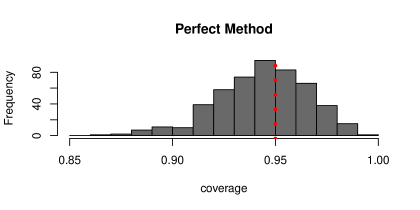
Figure 1: Histogram of the coverage probabilities of two sided 95% confidence intervals for 500 parameters. It illustrates how the results look like for a perfectly correct method for creating confidence intervals and one uses only 100 realizations to compute the probabilities.

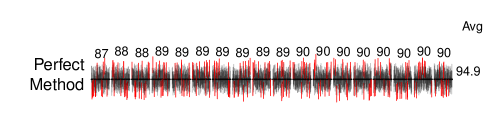
Figure 2: Plot of two sided 95% confidence intervals. It illustrates how the results would look like for a correct method for creating confidence intervals when one only computes 100 confidence intervals. 18 coefficients are chosen and are drawn in 18 columns from left to right with a black horizontal bar indicating the coefficient size. If any coefficients differ from zero then they are plotted first from the left (in order of decreasing magnitude). This particular example doesn’t exhibit any of those non-zero coefficients. The other coefficients are chosen to be those with the lowest coverage such that we can investigate potential causes for this poor coverage. The 100 computed confidence intervals are drawn from left to right in the column for the corresponding coefficient. The line segment is colored black in case it contains the truth, red otherwise. The number of confidence intervals that cover the truth for a particular coefficient is written above the confidence intervals in the respective column. The overall average coverage probability over all coefficients is displayed in the right-most column.

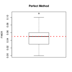
Figure 3: Plot of multiple testing performance in terms of familywise error rate (FWER) control. It illustrates how the results look like for a correct method for multiple testing correction, if one computes the error rates over 100 realizations of the model. The target is controlling the FWER at level $0.05$. This target is highlighted by a red-dotted horizontal line. We sample independent and identically distributed p-values $p_{j}\sim U(0,1)$, for $j=1,\dots,500$, and compute the familywise error rate over 100 realizations when using the rejection threshold $\alpha=0.05/500=0.0001$. The boxplot based on 300 data points is the result of repeating this experiment 300 times.

Of particular interest is the accuracy of the bootstrap when dealing with non-Gaussian and even heteroscedastic errors. For multiple testing, one would like to find out how much there is to gain when using the Westfall-Young procedure over a method that doesn’t exploit dependencies between the outcomes of the tests, such as Bonferroni-Holm. To this end, it is interesting to look at a variety of dependency structures for the design matrix and to look at real data as well.

For confidence intervals, we visualize the overall average coverage probability as well as the occurrence of too high or too low coverage probabilities. We work with histograms of the coverage probabilities for all coefficients in the model, as in example Figure 1. These probabilities are always computed based on 100 realizations of the corresponding linear model. For those cases where coverage is too low, we visualize the confidence intervals themselves to illustrate the poor coverage. An example of the plot we’ll work with can be found in Figure 2.

For multiple testing, we look at the power and the familywise error rate,

$$\mbox{Power}=\sum_{j\in S_{0}}\mathbb{P}[H_{0,j}\mbox{ is rejected}]/s_{0},$$

$$\mbox{FWER}=\mathbb{P}[\exists j\in S_{0}^{c}:H_{0,j}\mbox{ is rejected}],$$

where the probabilities are computed based on 100 realizations of the linear model.

We use boxplots to visualize the power and error rates, similar to Figure 3, where each data point is the result of the probability calculation described above. In order to generate interesting and representative data points, we look at different choices for the signal and different seeds for the data generation. As a rule, results for different design types are put in separate plots.

5.1 Varying the distribution of the errors

We first consider the performance of the bootstrap when varying the distribution of the errors for simulated data.

The design matrix will be generated $\sim\mathcal{N}_{p}(0,\Sigma)$ with a covariance matrix $\Sigma$ of two possible types (although mainly of Toeplitz type):

Toeplitz: $$\ \Sigma_{j,k}=0.9^{|j-k|}.$$

Independence: $$\ \Sigma=I_{p}.$$

In case the model contains signal, the coefficient vector will have $s_{0}=3$ coefficients that differ from zero. The coefficients are picked in 6 different ways:

$$\mbox{Randomly generated}:$$ U(0,2), U(0,4), U(-2,2),

$$\mbox{A fixed value}:$$ 1, 2 or 10.

5.1.1 Homoscedastic Gaussian errors

Data is generated from a linear model with Toeplitz design matrix and homoscedastic Gaussian errors of variance $\sigma^{2}=1$, $\varepsilon\sim\mathcal{N}_{n}(0,I_{n})$. The sample size is chosen to be $n=100$, the number of parameters $p=500$.

For confidence intervals, we focus on one generated design matrix $\mathbf{X}$ and one generated coefficient vector of type $U(-2,2)$. The histograms for the coverage probabilities can be found in Figure 4. The coverage probabilities are more correct for the bootstrapped estimator. The original estimator has a bias for quite a few coefficients resulting in low coverage, as can be seen in Figure 5. In addition, it tends to have too high coverage for many coefficients. The conservative RLDPE estimator has much wider confidence intervals which addresses the problem of low coverage but results in too high overall coverage.

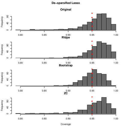
Figure 4: Histograms of the coverage probabilities of two-sided 95% confidence intervals for all $500$ parameters in a linear model ($n=100,p=500$), computed from 100 independent replications. Perfect performance would look like Figure 1. The fixed design matrix is of Toeplitz type, the single coefficient vector of type $U(-2,2)$ and homoscedastic Gaussian errors. The original estimator has more over-coverage and under-coverage than the bootstrapped estimator. The RLDPE estimator has little under-coverage, like the bootstrapped estimator, but it has too high coverage probabilities overall. The ZC approach to bootstrapping, which only bootstraps the linearized part of the estimator, doesn’t show any improvements over the original de-sparsified Lasso.

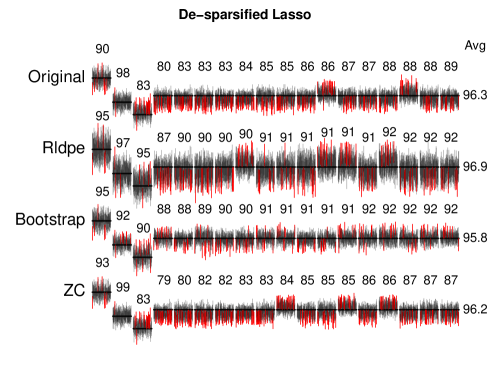
Figure 5: Two-sided 95% confidence intervals for the de-sparsified Lasso estimator. From left to right 18 coefficients are shown with a black horizontal bar of a certain height illustrating the value of the coefficient. Only the first three coefficients differ from zero. The other 15 coefficients presented are those with the lowest confidence interval coverage for that particular method (in decreasing order from left to right). 100 response vectors were generated for a linear model with homoscedastic Gaussian errors, fixed design of type Toeplitz, a single coefficient vector of type $U(-2,2)$, sample size $n=100$ and dimension $p=500$. Each of these realizations was fitted to produce a confidence interval for each coefficient in the model. The 100 confidence intervals are drawn as vertical lines and ordered from left to right in the column corresponding to that particular coefficient. The line segments are colored black if they cover the true coefficient and colored red otherwise. The number above each coefficient corresponds to the number of confidence intervals, out of 100, which end up covering the truth. The average coverage probability over all coefficients is provided in a column to the right of all coefficients. The original estimator has some bias for a few coefficients, which results in a lower than desired coverage for those coefficients. The RLDPE estimator has wider confidence intervals exhibiting over-coverage. The ZC approach to bootstrapping, which only bootstraps the linearized part of the estimator, doesn’t show any improvements over the original de-sparsified Lasso.

For multiple testing, we generate 50 Toeplitz design matrices $\mathbf{X}$ which are combined with 50 coefficient vectors for each coefficient type $U(0,2),U(0,4),U(-2,2),\mathrm{fixed\>}1,\mathrm{fixed\>}2$ and $\mathrm{fixed\>}10$. For each of these $300$ linear models, the coefficient vector undergoes a different random permutation. A value for the familywise error rate and power is then computed by generating 100 realizations of the linear models, as described in the introduction of Section 5. The boxplots of the power and familywise error rate can be found in Figure 6. The bootstrap is the least conservative option. In addition, one can conclude that it still has proper error control by comparing the results to perfect error control in Figure 3. One would expect to see a difference in power, but there doesn’t seem to be a visible difference between the bootstrap approach and the original estimator for our dataset. The RLDPE estimator, on the other hand, does turn out to be more conservative.

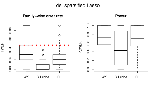
Figure 6: Boxplot of the familywise error rate and the power for multiple testing for the de-sparsified Lasso. The target is controlling the FWER at level $0.05$, highlighted by a red-dotted horizontal line. Two different approaches for multiple testing correction are compared, Westfall-Young (WY) and Bonferroni-Holm (BH). For Bonferroni-Holm, we make the distinction between the original method and the RLDPE approach. 300 linear models are investigated in total, where 50 Toeplitz design matrices are combined with 50 coefficient vectors for each of the 6 types $U(0,2),U(0,4),U(-2,2),\mathrm{fixed\>}1,\mathrm{fixed\>}2,\mathrm{fixed\>}10$. The variables belonging to the active set are chosen randomly. The errors in the linear model were chosen to be homoscedastic Gaussian. Each of the models has a data point for the error rate and the power in the boxplot. The error rate and power probabilities were calculated by averaging over 100 realizations.

5.1.2 Homoscedastic non-Gaussian errors

Data is generated from a linear model with Toeplitz design matrix and homoscedastic centered chi-squared errors $\varepsilon_{1},\ldots,\varepsilon_{n},$ of variance $\sigma^{2}=1$,

$$\zeta_{1},\ldots,\zeta_{n}\>\mbox{i.i.d.}\>\sim\chi_{1}^{2},\ \ \varepsilon_{i}=\frac{\zeta_{i}-1}{\sqrt{2}},\>\>\>i=1,\dots,n.$$

The sample size is chosen to be $n=100$, the number of parameters $p=500$.

For confidence intervals, we focus on one generated design matrix $\mathbf{X}$ and one generated coefficient vector of type $U(-2,2)$. The histograms for the coverage probabilities can be found in Figure 7.

The performance for the confidence intervals looks similar to that for Gaussian errors, only the under coverage of the original estimator is even more pronounced. The coverage for the bootstrapped estimator looks as good as in the Gaussian case. As can be seen in Figure 8, the cause for the poor coverage of the non-bootstrapped estimator is again bias. Using the robust standard error estimation doesn’t impact the results, as can be seen in Appendix A.4.

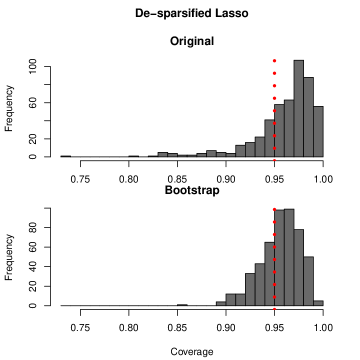
Figure 7: The same plot as Figure 4 but for homoscedastic chi-squared errors. The bootstrapped estimator has better coverage properties.

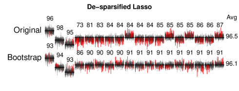
Figure 8: The same plot as Figure 5 but for homoscedastic chi-squared errors. The original estimator has quite some bias for a few coefficients, which results in a lower than desired coverage for those coefficients.

For multiple testing, the same setups were looked at as in Section 5.1.1 but now with the different errors. As can be seen in Figure 9, the poor single testing confidence interval coverage does not translate into poor multiple testing error control. The original method with Bonferroni-Holm is on the conservative side, while the bootstrap is slightly closer to the correct level.

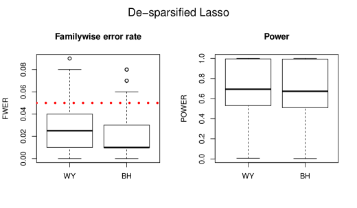
Figure 9: The same plot as Figure 6 but for homoscedastic chi-squared errors.

5.1.3 Heteroscedastic non-Gaussian errors

Data is generated from a linear model with heteroscedastic non-Gaussian errors. The example is taken from Mammen, (1993) with sample size $n=50$, but where we increased the number of parameters to $p=250$ from the original $p=5$. The model has no signal $\beta_{1}^{0}=\beta_{2}^{0}=\dots=\beta_{p}^{0}=0$ and introduces heteroscedasticity while still maintaining the correctness of the linear model.

Each row of the design matrix $\mathbf{X}$ is generated independently $\sim\mathcal{N}_{p}(0,I_{p})$ and then given a different variance. Each row is multiplied with the value $Z_{i}/2$, where the $\{Z_{1},\dots,Z_{n}\}$ are chosen i.i.d. $\sim U(1,3)$.

The errors $\varepsilon_{i}$ are chosen to be a mixture of normal distributions

$$\varepsilon_{1},\ldots,\varepsilon_{n}\ \mbox{i.i.d},\ \varepsilon_{i}=l_{i}\zeta_{i}+(l_{i}-1)\eta_{i},$$

$$l_{i}\sim\operatorname{Bernoulli}(0.5),\ \zeta_{i}\sim\mathcal{N}(1/2,(1.2)^{2}),\ \eta_{i}\sim\mathcal{N}(-1/2,(0.7)^{2}),$$

with $l_{i},\ \zeta_{i},\ \eta_{i}$ independent of each other. The responses are generated by introducing heteroscedasticity in the errors

$$Y_{i}=Q_{i}\varepsilon_{i}+\varepsilon_{i}\>\>\>\>\>\>\forall i=1,\ldots,n$$

with $Q_{i}=X_{i,1}^{2}+X_{i,2}^{2}+X_{i,3}^{2}+X_{i,4}^{2}+X_{i,5}^{2}-\mathbb{E}[Z_{i}^{2}]$.

For confidence intervals, we focus on one generated design matrix $\mathbf{X}$. The histograms for the coverage probabilities can be found in Figure 10, the plot of the actual confidence intervals is shown in Figure 11. What is immediately clear from Figure 10 is that it makes a big difference if one uses the robust version of the standard error estimation or not. The coverage is very poor for the non-robust methods, while for the robust methods the performance looks like perfect coverage (Figure 1).

There isn’t any benefit for the bootstrap over the original estimator for this dataset. The robust original estimator doesn’t show any bias in Figure 11 and has great coverage already. The overall average coverage is slightly more correct for the bootstrap with a value of 95.1 versus 95.9.

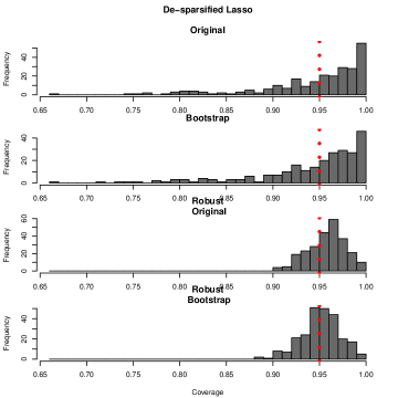
Figure 10: The same plot as Figure 4 but for heteroscedastic non-Gaussian errors and without signal. The robust standard error estimation clearly outperforms the non-robust version. There seems to be hardly any difference between the bootstrap and the original estimator after choosing the standard error estimation.

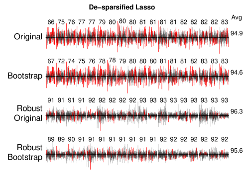
Figure 11: The same plot as Figure 5 but for heteroscedastic non-Gaussian errors and without signal. The non-robust estimators have low coverage for many coefficients. Unlike the other setups, there doesn’t seem to be a bias in the original estimator for this dataset.

In contrast to the single testing confidence intervals, all methods (robust and non-robust) perform adequately for multiple testing as can be seen in Figure 9. Due to the lack of signal in the dataset, we can only investigate error rates. 50 different design matrices were generated to produce the 50 data points in the boxplots. The bootstrap is less conservative and has actual error rate closer to the true level.

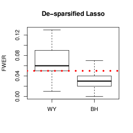
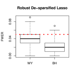
Figure 12: The same plot as Figure 6 but for heteroscedastic non-Gaussian errors and without signal. We only report the error rate because all null hypotheses are true for the generated dataset. The plot on the left is for the non-robust methods, the one on the right for the robust ones.

5.1.4 Discussion

Bootstrapping the de-sparsified Lasso turns out to improve the coverage of confidence intervals without increasing the confidence interval lengths (that is, without loosing efficiency). The use of the conservative RLDPE (Zhang and Zhang,, 2014) is not necessary: the bootstrap achieves reliable coverage, while for the original de-sparsified Lasso, the RLDPE seems worthwhile to achieve reasonable coverage while paying a price in terms of efficiency. Furthermore, bootstrapping only the linearized part of the de-sparsified estimator as proposed by Zhang and Cheng, (2016) is clearly sub-ideal in comparison to bootstrapping the entire estimator and using the plug-in principle as advocated here.

For multiple testing, the bootstrapped estimator had familywise error rates that were closer to the target level while Bonferroni-Holm adjustment is too conservative. This finding was not reflected in any noticeable power improvements but some gains are found, see Section 5.2 below.

The robust standard error turned out to be critical when dealing with heteroscedastic errors. Therefore, we recommend the bootstrapped estimator with robust standard error estimation as the method to be used: if the errors were homoscedastic, we pay a price of efficiency; see also the sentence at the end of Section 5.2.1.

As can be seen in Appendix A.4.2, the Gaussian multiplier bootstrap also performs well. The performance is very similar to the residual bootstrap and, as one would expect, it handles heteroscedastic errors as good as the robust standard error bootstrap approach.

5.2 A closer look at multiple testing

The examples from Section 5.1 showed little to no power difference between the bootstrap and the original estimator. One straightforward explanation for this is that the signal in the simulated datasets didn’t fall into the (possibly small) differences in rejection regions.

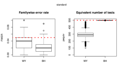
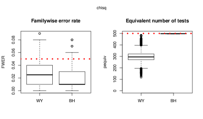
Figure 13: The same plots as Figure 6 for the homoscedastic Gaussian errors (top) and Figure 9 for the homoscedastic non-Gaussian errors (bottom), but displaying the number of equivalent tests $p_{equiv}$ instead of the power. The actual number of hypotheses tested is highlighted by a red dotted horizontal line.

As another more signal-independent way to investigate multiple testing performance, we compare the computed rejection regions. Unfortunately, the actual values of the rejection thresholds are often quite unintuitive to compare. Instead, it can be more informative to invert the Bonferroni-Holm adjustment rule to compute some equivalent number of tests which is essentially equivalent to the number of tests under independence. The Westfall-Young procedure computes a rejection threshold $t_{rej}$ for the absolute value of the test statistic and we can then compute the equivalent number of tests (with the Bonferroni adjustment) $p_{equiv}$ as

$$p_{equiv}=\frac{\alpha}{2(1-\Phi(t_{rej}))},$$ (15)

for controlling the familywise error rate at level $\alpha$, and with $\Phi(.)$ the cumulative distribution function for $\mathcal{N}(0,1)$. Improvements in rejection threshold are then reflected in $p_{equiv}$ being a lot smaller than the actual number of hypotheses tested $p$, while still properly controlling the error rates.

Looking at the rejection thresholds presented in Figure 13, we can see that the bootstrap does improve substantially over the original estimator with a Bonferroni correction. Multiple testing with the bootstrap is often equivalent to testing about 300 (independent) tests with Bonferroni correction in comparison to the original 500.

5.2.1 Real measurements design

We take design matrices from real data and simulate a linear model with known signal and homoscedastic Gaussian errors. We look at all 6 signal options described in Section 5.1.

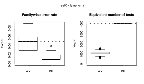
Figure 14: The same plot as in Figure 13 but with design matrix coming from real measurements (lymphoma in this case) with simulated signal and homoscedastic Gaussian errors.

For every signal type, we only look at 5 different seeds for generating the coefficients and for the permutations of the coefficient vector (in contrast to the typical 50 as used in Section 5.1.1). As usual, the familywise error rates are computed based on 100 realizations of each model.

Boxplots of the familywise error rate and $p_{equiv}$ for the lymphoma dataset can be found in Figure 14. The median values of the equivalent number of tests and the FWER for all the different designs are as follows:

	dsmN71	brain	breast	lymphoma	leukemia	colon	prostate	nci
Median $p_{equiv}$ WY	1264	886	1162	1083	1230	655	2466	1289
Median $p_{equiv}$ BH	4088	5596	7129	4025	3570	2000	6032	5243
Dimension p	4088	5597	7129	4026	3571	2000	6033	5244
Median FWER WY	0.02	0.06	0.05	0.05	0.05	0.03	0.06	0.03
Median FWER BH	0.00	0.02	0.01	0.01	0.03	0.00	0.04	0.01

The bootstrap achieves substantial reductions in the median equivalent number of tests for all datasets investigated here.

We note that when studentizing the test-statistics with the robust standard error, the power gain with the bootstrap (Westfall-Young method) is often rather marginal. This is illustrated in Appendix A.4.1.

5.2.2 Real data example

We revisit a dataset about riboflavin production by bacillus subtilis (Bühlmann et al.,, 2014), already studied in Bühlmann, (2013), van de Geer et al., (2014) and Dezeure et al., (2015). The dataset has dimensions $n=71$ $p=4088$ and the original de-sparsified Lasso doesn’t manage to reject any null hypothesis $H_{0,j}$ at the 5% significance level after multiple testing correction with Bonferroni-Holm.

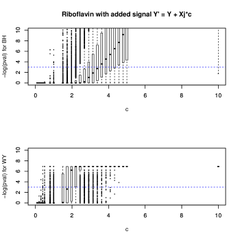
Figure 15: Multiple testing corrected p-values for increasing artificial signal added to the real dataset Riboflavin (dsmN71). Signal is added only one variable at a time $Y^{{}^{\prime}}=Y+X_{j}c$, and only the p-value for that coefficient $p_{j}$ is stored for each such experiment and value of $c$. The values $-\log(p_{j})$ for all different experiments ($j=1,\dots,p=4088$) are plotted in boxplots grouped by value of $c$. A horizontal dashed blue line indicates the rejection threshold $0.05$. The bootstrap approach to multiple testing clearly has higher power as it picks up on the signal quicker. The bootstrap has a lower bound on the minimal achievable p-value due to the finite number of bootstrap samples $B=1000$, namely $-\log(1/1000)\approx 6.9$.

Despite the power gain that is possible with this design matrix (see dsmN71 in the Table in Section 5.2.1) , the bootstrapped estimator doesn’t reject any hypotheses either with the Westfall-Young procedure.

We investigate what signal strength one would be able to detect in this real dataset by adding artificial signal to the original responses. This is done by adding a linear component $X_{j}c$ of increasing signal strength c for a single variable $j$,

$$Y^{{}^{\prime}}=Y+X_{j}c.$$

One can keep track of the p-value for this particular coefficient and repeat the experiment for all possible columns of the design $j=1,\dots,p$. Boxplots of this experiment can be found in Figure 15.

The bootstrap results in smaller p-values for the same signal values. It rejects the relevant null hypothesis almost all the time for signal values above $c>2.5$. Note that we do not have access to replicates and therefore, we cannot determine the actual error rate.

5.2.3 Discussion

The bootstrap with the Westfall-Young (WY) multiple testing adjustment leads to reliable familywise error control while providing a rejection threshold which is far more powerful than using the Bonferroni adjustment (in the case of homoscedastic errors), especially in presence of dependence among the components for testing (while for heteroscedastic errors and when using the robust standard error for studentization, the efficiency gain of WY often seems less substantial). Since the efficient WY adjustment is not adding additional computational costs to the one from bootstrapping, such simultaneous inference and WY multiple testing adjustment is highly recommended.

6 Further considerations

We discuss here additional points before providing some conclusions.

6.1 Model misspecification

So far, the entire discussion has been for a linear model as in (1) with a sparse regression vector $\beta^{0}$. The linearity is not really a restriction: suppose that the true model would involve a nonlinear regression function

$$Y_{i}=f^{0}(X_{i})+\varepsilon_{i}\ (i=1,\ldots n).$$

The $n\times 1$ vector of the true function at the observed data values $(f^{0}(X_{1}),\ldots,f^{0}(X_{n}))^{T}$ can be represented as

$$(f^{0}(X_{1}),\ldots,f^{0}(X_{n}))^{T}=\mathbf{X}\beta^{0}$$ (16)

for many possible solutions $\beta^{0}$: this is always true as long as $\mathrm{rank}(\mathbf{X})=n$ which typically holds in $p\geq n$ settings. The issue is whether there are solutions $\beta^{0}$ in (16) which are sparse: a general result to address this point is not available, see Bühlmann and van de Geer, (2015).

It is argued in Bühlmann and van de Geer, (2015) that weak sparsity in terms of $\|\beta^{0}\|_{r}$ for $0<r<1$ suffices to guarantee that the de-sparsified Lasso has an asymptotic Gaussian distribution centered at $\beta^{0}$, as described in Theorem 1 or 2. Thus, assuming that there is a weakly sparse solution $\beta^{0}$ in (16) is relaxing the requirement for $\ell_{0}$ sparsity. The presented theory for the bootstrap could be adapted to cover the case for weakly sparse $\beta^{0}$.

The interpretation of a confidence interval for $\beta^{0}$, based on the Gaussian limiting distribution of the de-sparsified Lasso or using its bootstrapped version as described in this paper, is that it covers all $\ell_{r}\ (0<r<1)$ weakly sparse solutions $\beta^{0}$ which are solutions of (16). Thereby, we implicitly assume that there is at least one such $\ell_{r}$ weakly sparse solution.

6.2 Random design

The distinction between fixed and random design becomes crucial for misspecified models. If the true model with random design is linear, then by conditioning on the covariables, the corresponding fixed design model is again linear. And if the inference is correct conditional on $\mathbf{X}$, it is also correct unconditional for random design. If the true random design model is nonlinear, one can look at the best projected random design linear model: but then, when conditioning, the obtained projected fixed design linear model has a bias (or non-zero conditional mean for the error). In other words, conditioning on the covariables is not appropriate when the model is wrong, and one should rather do unconditional inference in a random design (best approximating) linear model; see Bühlmann and van de Geer, (2015).

Thus, there are certainly situations where one would like to do unconditional inference in a random design linear model, see also Freedman, (1981) who proposes the “paired bootstrap” in a low-dimensional setting. The bootstrap which we discussed in this paper is for fixed design only: for random design, one should resample the covariables as well. Because of the latter the computational task becomes much more demanding: for the de-sparsified Lasso, and when $p$ is large, most of the computation is spent on computing all the residual vectors $Z_{1},\ldots,Z_{p}$ which requires running the Lasso $p$ times. For bootstrapping with fixed design, this computation has to be done only once (since $Z_{1},\ldots,Z_{p}$ are deterministic values of the fixed design $\mathbf{X}$); with random design, it seems unavoidable to do it $B\approx 100-1^{\prime}000$ times which would result in a major additional computational cost.

6.3 Conclusions

We propose a residual, wild and paired bootstrap methodology for individual and simultaneous inference in high-dimensional linear models with possibly non-Gaussian and heteroscedastic errors. The bootstrap is used to approximate the distribution of the de-sparsified Lasso, a regular non-sparse estimator which is not exposed to the unpleasant super-efficiency phenomenon.

We establish asymptotic consistency for possibly simultaneous inference for parameters in a group $G\subseteq\{1,\ldots,p\}$ of variables, where $p\gg n$ but $s_{0}=o(n^{1/2}/\{\log(p)\log(|G|)\})$ and $\log(|G|)=o(n^{1/7})$ with $s_{0}$ denoting the sparsity. The presented general theory is complemented by many empirical results, demonstrating the advantages of our approach over other proposals. Especially for simultaneous inference and multiple testing adjustment, the bootstrap is very powerful.

For homoscedastic errors, the residual and wild bootstrap perform similarly. For heteroscedastic errors, the wild bootstrap is more natural and can be used for simultaneous inference (whereas the residual bootstrap fails to be consistent). Thus, for protecting against heteroscedastic errors, the wild bootstrap seems to be the preferred method. Our proposed procedures are implemented in the R-package hdi (Meier et al.,, 2016).

Acknowledgments.

We gratefully acknowledge visits at the American Institute of Mathematics (AIM), San Jose, US, and at the Mathematisches Forschungsinstitut (MFO), Oberwolfach, Germany.

Appendix A Appendix

We present here all the proofs and additional empirical results.

The proof is composed of four propositions, stating the consistency of variance estimates and Gaussian approximation of studentized statistics for the original estimator, paired bootstrap, wild bootstrap and xyz-paired bootstrap. The theorems then follow directly from the corresponding propositions.

The following notation will be used. For any vectors $u=(u_{1},\ldots,u_{n})^{T}$ and $v=(v_{1},\ldots,v_{n})^{T}$, denote the mean of $u$ by ${\overline{u}}=n^{-1}\sum_{i=1}^{n}u_{i}$, the centered $u$ by $u_{\rm cent}=(u_{1}-{\overline{u}},\ldots,u_{n}-{\overline{u}})^{T}$, and the Hadamard product by $u\circ v=(u_{1}v_{1},\ldots,u_{n}v_{n})^{T}$.

A.1 Proof of Theorem 1 for homoscedastic errors

We remark first that the variance estimator in (2.2) is asymptotically equivalent to $\hat{\sigma}_{\varepsilon}^{2}=n^{-1}\sum_{i=1}^{n}(Y_{i}-(\mathbf{X}\hat{\beta})_{i})^{2}$ if $\hat{s}=O(s_{0})=o(n)$. The latter holds under the assumption (B3) (which, together with other assumptions, ensures (A4)). For simplicity of the proofs, we consider here this modified variance estimator with the factor $n^{-1}$.

We first collect in the following proposition results on the original estimator in the more general heteroscedastic case. This will allow us to apply the proposition to the plug-in bootstrap estimator by checking the assumptions of the proposition under probability measure ${\mathbb{P}}^{*}$ for each bootstrap method. The proposition allows $\mathbf{X}$ and $(Z_{j},j\in G)$ to be random and dependent on the noise $\varepsilon$, so that it can be applied to the xyz-paired bootstrap. To this end, we replace assumptions (A2), (A3), (A5) and (A6) by the following:

(A2dep)

$\displaystyle\max_{k\neq j}\frac{|Z_{j}^{T}X_{k}|^{2}}{n{\mathbb{E}}\|Z_{j}\|_{2}^{2}}\leq\lambda_{X}^{2},{\mathbb{E}}[Z_{j}\circ\varepsilon]=0,\frac{{\mathbb{E}}\|\varepsilon\circ Z_{j}\|_{2}^{2}}{n\vee{\mathbb{E}}\|Z_{j}\|_{2}^{2}}\geq L,\frac{{\mathbb{E}}\|\varepsilon\circ Z_{j}\|_{2+\delta}^{2+\delta}}{({\mathbb{E}}\|\varepsilon\circ Z_{j}\|_{2}^{2})^{1+\delta/2}}\ll 1,\ \forall j\in G$.

(A3dep)

$(X_{ik},k\leq p,\varepsilon_{i},Z_{j,i},j\in G)$ independent, $\mathbb{E}[\varepsilon]=0$, $\mathbb{E}\|\varepsilon\|_{2}^{2}/n=\sigma_{\varepsilon}^{2}$, $\mathbb{E}\|\varepsilon\|_{2+\delta}^{2+\delta}/n\leq C$.

(A5dep)

$\max_{j\leq p}\|X_{j}\|_{\infty}\leq C_{X}$, ${\mathbb{E}}[X_{j}\circ\varepsilon]=0$ for all $j\leq p$.

(A6dep)

$\max_{j\in G}\|Z_{j}\|_{\infty}\leq K$, $\max_{1\leq i\leq n}{\mathbb{E}}\,\varepsilon_{i}^{2}=O(n^{3/7})$, $\delta=2$, $\log(2|G|)\ll n^{1/7}$.

Again, $\sigma_{\varepsilon}$, $L$, $C$, $C_{X}$ and $K$ are positive constants bounded away from $0$ and $\infty$, $\delta\in(0,2]$ is fixed and the same in (A2dep) and (A3dep), and $\lambda_{X}\asymp\sqrt{\log(p)/n}$. It is clear that when $\mathbf{X}$ and $(Z_{j},j\in G)$ are deterministic, (A2), (A3) and (A5) directly imply (A2dep), (A3dep) and (A5dep), and (A3) and (A6) directly imply the first two requirements in (A6dep). We generalize $\omega_{j}$ and define $\omega_{j,k}$ as

$$\omega_{j}=\sqrt{{\mathbb{E}}\|\varepsilon\circ Z_{j}\|_{2}^{2}/n},\quad\omega_{j,k}={\mathbb{E}}(\varepsilon\circ Z_{j})^{T}(\varepsilon\circ Z_{k})/n.$$

Let $(\zeta_{j},j=1,\ldots,p)$ be a Gaussian vector with

$${\mathbb{E}}\,\zeta_{j}=0,\ {\mathbb{E}}\,\zeta_{j}\zeta_{k}=\frac{\omega_{j,k}}{\omega_{j}\omega_{k}}=\hbox{\rm corr}\Big{(}\varepsilon\circ Z_{j},\varepsilon\circ Z_{k}\Big{)}.$$

Proposition 1.

Assume (A1), (A2dep), (A3dep) and (A5dep). Then,

$$|\widehat{s.e.}_{j}/{s.e.}_{j}-1|=|{\hat{\sigma}}_{\varepsilon}/\sigma_{\varepsilon}-1|=O_{P}(n^{-{\delta}/(2+{\delta})})+o_{P}(1)\big{/}\big{\{}\log(p)\log(2|G|)\big{\}},\ \forall j\leq p,$$

$$\left|\widehat{s.e.}_{\mathrm{robust},j}/s.e._{\mathrm{robust},j}-1\right|=\left|\hat{\omega}_{j}/\omega_{j}-1\right|=o_{P}(1)\ \hbox{for each $j\in G$.}$$

Let $T_{j}=\hbox{\rm sgn}(Z_{j}^{T}X_{j})({\hat{b}}_{j}-\beta_{j}^{0})/\widehat{s.e.}_{\mathrm{robust},j}$. If $|G|=O(1)$, then

$$\sup_{(t_{j},j\in G)}\Big{|}{\mathbb{P}}\left[T_{j}\leq t_{j},j\in G\right]-{\mathbb{P}}\left[\zeta_{j}\leq t_{j},j\in G\right]\Big{|}=o_{P}(1).$$ (17)

If (A6dep) holds, then $\max_{j\in G}\left|\hat{\omega}_{j}/\omega_{j}-1\right|=o_{P}(1)/\log^{2}(2|G|)$ and

$$\sup_{c\in\mathbb{R}}\big{|}\mathbb{P}\big{[}\max_{j\in G}h_{j}(T_{j})\leq c\big{]}-\mathbb{P}\big{[}\max_{j\in G}h_{j}(\zeta_{j})\leq c\big{]}\big{|}=o(1)$$ (18)

for any combination of functions $h_{j}(t)=t$, $h_{j}(t)=-t$ or $h_{j}(t)=|t|$. Moreover, (17) and (18) hold under respective assumptions for $T_{j}=\hbox{\rm sgn}(Z_{j}^{T}X_{j})({\hat{b}}_{j}-\beta_{j}^{0})/\widehat{s.e.}_{j}$ in the homoscedastic case where ${\mathbb{E}}[\varepsilon_{i}|Z_{j},j\in G]=0$ and ${\mathbb{E}}[\varepsilon_{i}^{2}|Z_{j},j\in G]=\sigma_{\varepsilon}^{2}$ for all $i\leq n$.

Although $\widehat{s.e.}_{j}$ is a consistent estimator of ${s.e.}_{j}$, $\widehat{s.e.}_{j}\neq s.e._{\mathrm{robust},j}$ in general. Thus, $\widehat{s.e.}_{j}$ may not properly normalize ${\hat{b}}_{j}$ without the homoscedasticity assumption. Meanwhile, $\widehat{s.e.}_{j}^{*}$ always properly normalize the residual bootstrapped ${\hat{b}}^{*}_{j}$ as stated later in Proposition 2.

Proof: It follows from (A3dep) and the Marcinkiewicz-Zygmund inequality that

$${\mathbb{E}}\Big{|}\,\|\varepsilon\|_{2}^{2}-n\sigma^{2}_{\varepsilon}\Big{|}^{(1+\delta/2)}=O(1){\mathbb{E}}\Big{|}\sum_{i=1}^{n}(\varepsilon_{i}^{2}-{\mathbb{E}}\varepsilon_{i}^{2})^{2}\Big{|}^{1/2+\delta/4}=O(1){\mathbb{E}}\|\varepsilon\|_{2+\delta}^{2+\delta}=O(n).$$ (19)

Because Nemirovski’s inequality still applies as in Ex.14.3 of Bühlmann and van de Geer, (2011) under the weaker assumptions (A3dep) and (A5dep),

$${\mathbb{E}}\|\mathbf{X}^{T}\varepsilon\|_{\infty}\leq O(C_{X}\sqrt{\log p})\sqrt{{\mathbb{E}}\|\varepsilon\|_{2}^{2}}=O(\sqrt{n\log p}).$$ (20)

As ${\hat{\varepsilon}}-\varepsilon=\mathbf{X}({\hat{\beta}}-\beta^{0})$, $|\varepsilon^{T}({\hat{\varepsilon}}-\varepsilon)|\leq\|\mathbf{X}^{T}\varepsilon\|_{\infty}\|{\hat{\beta}}-\beta^{0}\|_{1}=o_{P}(n^{1/2})$ by (A1). By (A1) and (A5dep),

$$\|{\hat{\varepsilon}}_{\rm cent}-\varepsilon\|_{\infty}\vee\|{\hat{\varepsilon}}-\varepsilon\|_{\infty}\leq\big{|}{\overline{\varepsilon}}\big{|}+2\|\mathbf{X}\|_{\infty}\|{\hat{\beta}}-\beta^{0}\|_{1}\leq O_{P}(n^{-1/2})+o_{P}(1)/\sqrt{\log(p)\log(2|G|)}.$$ (21)

This and (19) yield the first statement as $\widehat{s.e.}_{j}/{s.e.}_{j}={\hat{\sigma}}_{\varepsilon}/\sigma_{\varepsilon}$ and ${\hat{\sigma}}_{\varepsilon}^{2}=\|{\hat{\varepsilon}}\|_{2}^{2}/n$ by definition.

The second statement follows in the same manner by (21), (A2dep) and

$${\mathbb{E}}\Big{|}\,\|\varepsilon\circ Z_{j}\|_{2}^{2}-n\omega_{j}^{2}\Big{|}^{(1+\delta/2)}=O(1){\mathbb{E}}\|\varepsilon\circ Z_{j}\|_{2+\delta}^{2+\delta}=o\big{(}(n\omega_{j}^{2})^{1+\delta/2}\big{)}.$$ (22)

For the normal approximation (17) and (18), define

$$\xi_{i,j}=\frac{Z_{j;i}^{T}\varepsilon_{i}}{\omega_{j}},\quad\xi_{j}=\sum_{i=1}^{n}\frac{\xi_{i,j}}{n^{1/2}}=\frac{Z_{j}^{T}\varepsilon}{n^{1/2}\omega_{j}}.$$

By (A3dep) and (A2dep), $\{Z_{j;i}\varepsilon_{i},i\leq n\}$ are independent variables satisfying the Lyapunov condition, so that $\xi_{j}\to N(0,1)$. Furthermore, for $|G|=O(1)$, any linear combination $\sum_{j\in G}a_{j}\xi_{j}$ converges in distribution to the corresponding Gaussian linear combination $\sum_{j\in G}a_{j}\zeta_{j}$ by the Lyapunov CLT when ${\mathbb{E}}(\sum_{j\in G}a_{j}\zeta_{j})^{2}>0$ and converges in probability to $\sum_{j\in G}a_{j}\zeta_{j}=0$ otherwise. Because $\mbox{Var}(\zeta_{j})=1$, this is equivalent to

$$\sup_{(t_{j},j\in G)}\Big{|}{\mathbb{P}}\left[\xi_{j}\leq t_{j},j\in G\right]-{\mathbb{P}}\left[\zeta_{j}\leq t_{j},j\in G\right]\Big{|}=o_{P}(1).$$ (23)

Next we bound $T_{j}-\xi_{j}$. Let $\Delta_{j}^{(1)}=\sum_{k\neq j}Z_{j}^{T}X_{k}(\beta^{0}_{k}-{\hat{\beta}}_{k})/(\sqrt{n}{\hat{\omega}}_{j})$. By (2),

$${\hat{b}}_{j}-\beta_{j}^{0}=\frac{Z_{j}^{T}Y}{Z_{j}^{T}X_{j}}-\sum_{k\neq j}\frac{Z_{j}^{T}X_{k}}{Z_{j}^{T}X_{j}}{\hat{\beta}}_{k}-\beta_{j}^{0}=\frac{Z_{j}^{T}\varepsilon+\Delta_{j}^{(1)}\sqrt{n}{\hat{\omega}}_{j}}{Z_{j}^{T}X_{j}}.$$

Let $\Delta_{j}^{(2)}=(\omega_{j}/{\hat{\omega}}_{j}-1)\xi_{j}$. By the definition of $\widehat{s.e.}_{\mathrm{robust},j}$ and simple algebra,

$$T_{j}=\frac{Z_{j}^{T}\varepsilon+\Delta_{j}^{(1)}\sqrt{n}{\hat{\omega}}_{j}}{\sqrt{n}{\hat{\omega}}_{j}}=\xi_{j}+\Delta_{j}^{(1)}+\Delta_{j}^{(2)}.$$

It follows from (A1), the first requirement in (A2dep), the consistency of ${\hat{\omega}}_{j}$ and (23) that

$$\max_{j\in G}\left|T_{j}-\xi_{j}\right|=\max_{j\in G}\Big{|}\Delta_{j}^{(1)}+\Delta_{j}^{(2)}\Big{|}=O_{P}\big{(}\sqrt{n}\lambda_{X}\|{\hat{\beta}}-\beta^{0}\|_{1}\big{)}+o_{P}(1)=o_{P}(1).$$

This and (23) yield the CLT (17) for $\{T_{j},j\in G\}$.

Now we impose the additional assumption (A6dep). We note that

$$L\leq\omega_{j}^{2}={\mathbb{E}}\|\varepsilon\circ Z_{j}\|_{2}^{2}/n\leq K^{2}C^{1/(1+\delta/2)}$$ (24)

by (A2dep), (A3dep) and (A6dep). Again, as ${\mathbb{E}}\|\varepsilon\|_{4}^{4}/n\leq C$, Nemirovski’s inequality gives

$${\mathbb{E}}\max_{j,k\in G}\Big{|}(\varepsilon\circ Z_{j})^{T}(\varepsilon\circ Z_{k})^{T}-n\omega_{j,k}\Big{|}\leq K^{2}\sqrt{8Cn\log(2|G|)},$$ (25)

$$\max_{j\in G}\Big{|}(\varepsilon\circ Z_{j})^{T}(({\hat{\varepsilon}}-\varepsilon)\circ Z_{j}))^{T}\Big{|}\leq\max_{j,k}\big{|}(Z_{j}\circ Z_{j}\circ X_{k})^{T}\varepsilon\big{|}\,\|{\hat{\beta}}-\beta^{0}\|_{1}=o_{P}(n^{1/2}).$$

As $\|({\hat{\varepsilon}}-\varepsilon)\circ Z_{j}\|_{2}^{2}/n\leq O_{P}(\|{\hat{\varepsilon}}-\varepsilon\|_{\infty}^{2})=o_{P}(1)/\{\log p\log(2|G|)\}$, we have

$$|{\hat{\omega}}_{j}^{2}/\omega_{j}^{2}-1|=O_{P}\big{(}\sqrt{\log(2|G|)/n}\big{)}+\frac{o_{P}(1)}{\log p\log(2|G|)}=o_{P}\big{(}\log^{-2}(2|G|)\big{)}.$$

Moreover, as ${\mathbb{E}}\max_{j\in G}|Z_{j}^{T}\varepsilon/\sqrt{n}|=O(\sqrt{\log(2|G|)})$,

$$\max_{j\in G}\left|T_{j}-\xi_{j}\right|\leq O_{P}\big{(}\sqrt{n}\lambda_{X}\|{\hat{\beta}}-\beta^{0}\|_{1}\big{)}+\frac{o_{P}(1)}{\log^{3/2}(2|G|)}=\frac{o_{P}(1)}{\sqrt{\log(2|G|)}}.$$ (26)

To prove (18), we note that the covariance structure of $\xi_{j}$ is the same as that of $\zeta_{j}$,

$${\mathbb{E}}\big{(}\xi_{j}\xi_{k}\big{)}=\frac{1}{n}\sum_{i=1}^{n}{\mathbb{E}}\big{(}\xi_{i,j}\xi_{i,k}\big{)}=\frac{{\mathbb{E}}(\varepsilon\circ Z_{j})^{T}(\varepsilon\circ Z_{k})}{n\omega_{j}\omega_{k}}={\mathbb{E}}\,\zeta_{j}\zeta_{k}.$$

The anti-concentration inequality in Lemma 2.1 of Chernozhukov et al., (2013) asserts that

$$\Delta=\frac{o(1)}{\log^{1/2}(2|G|)}\ \Rightarrow\ \sup_{c\in\mathbb{R}}\mathbb{P}\big{[}c\leq\max_{j\in G}h_{j}(\zeta_{j})\leq c+\Delta\big{]}=o(1).$$

Thus, as the differences $T_{j}-\xi_{j}$ are negligible by (26), (18) is a consequence of

$$\sup_{c\in\mathbb{R}}\big{|}\mathbb{P}\big{[}\max_{j\in G}h_{j}(\xi_{j})\leq c\big{]}-\mathbb{P}\big{[}\max_{j\in G}h_{j}(\zeta_{j})\leq c\big{]}\big{|}=o(1).$$ (27)

Moreover, (27) can be established by Theorem 2 in Chernozhukov et al., (2013) provided proper fourth moments and $\ell_{\infty}$ bounds for $\xi_{i,j}$ exist. As $|\xi_{j}|=\max(\xi_{j},-\xi_{j})$, $h_{j}(t)=|t|$ is allowed.

Because $\delta=2$ under (A6dep), (A6dep) and (A3dep) provide the fourth moment bound

$$\max_{j\in G}{\mathbb{E}}\sum_{i=1}^{n}\frac{|\xi_{i,j}|^{4}}{n}=\max_{j\in G}\frac{1}{n}{\mathbb{E}}\sum_{i=1}^{n}\left|\frac{Z_{j,i}\varepsilon_{i}}{\omega_{j}}\right|^{4}\leq\frac{K^{4}{\mathbb{E}}\|\varepsilon\|_{4}^{4}}{n\omega_{j}^{4}}=O(1).$$

Thus, for any $\ell_{\infty}$ bound $u(\gamma)=u(\gamma,X,Y)$ satisfying

$$\max\left\{{\mathbb{P}}\Big{[}\max_{i\leq n,j\in G}|\xi_{i,j}|>u(\gamma)\Big{]},\sum_{i\leq n,j\in G}{\mathbb{P}}\left[N\left(0,\frac{{\mathbb{E}}(Z_{j,i}\varepsilon_{i})^{2}}{\omega_{j}^{2}}\right)>u(\gamma)\right]\right\}\leq\gamma,$$

Theorem 2 of Chernozhukov et al., (2013) asserts that the left-hand side of (27) is no grater than

$$O(1)\left\{n^{-1/8}(\log(|G|n/\gamma))^{7/8}+n^{-1/2}(\log(|G|n/\gamma))^{3/2}u(\gamma)+\gamma\right\}.$$

Similar to the bound for the fourth moment, we have

$${\mathbb{E}}\max_{i\leq n,j\in G}|\xi_{i,j}|={\mathbb{E}}\left(\max_{i\leq n,j\in G}\frac{|Z_{j,i}\varepsilon_{i}|}{\omega_{j}}\right)=O({\mathbb{E}}\|\varepsilon\|_{4})=O(n^{1/4}).$$

By (A6dep), $\max_{j\in G}{\mathbb{E}}(Z_{j,i}\varepsilon_{i})^{2}/\omega_{j}^{2}=O(1)\max_{i\leq n}{\mathbb{E}}\varepsilon_{i}^{2}=O(n^{3/7})$. These $\ell_{\infty}$ bounds provide

$$u(\gamma)=O(1)\big{\{}n^{1/4}+n^{3/14}\log^{1/2}(n|G|)\big{\}}$$

for certain $\gamma=o(1)$. Thus, (27) holds via the conditions $\log(|G|)\ll n^{1/7}$. $\Box$

As a next step, we present the counter part of Proposition 1 for the residual bootstrap.

Proposition 2.

Assume (A1)-(A5) with ${\mathbb{E}}\varepsilon_{i}^{2}=\sigma^{2}_{\varepsilon}$ for all $i\leq n$. Let ${\mathbb{P}}^{*}$ represent the residual bootstrap of $\hat{\varepsilon}_{\mathrm{cent}}$. Then, ${s.e.}_{j}=s.e._{\mathrm{robust},j}$,

$$\displaystyle\widehat{s.e.}_{j}^{*}/{s.e.}_{j}={\hat{\sigma}}_{\varepsilon}^{*}/\sigma_{\varepsilon}=1+\frac{O_{P^{*}}}{n^{{\delta}/(2+{\delta})}}+\frac{o_{P^{*}}(1)}{\log(p)\log(2|G|)}\ \forall j\leq p\hbox{ in probability,}$$

$$\left|\widehat{s.e.}_{\mathrm{robust},j}^{*}/s.e._{\mathrm{robust},j}-1\right|=\left|\hat{\omega}_{j}^{*}/\omega_{j}-1\right|=o_{P^{*}}(1)\ \hbox{in probability for each $j\in G$.}$$

Let $T_{j}^{*}=\hbox{\rm sgn}(Z_{j}^{T}X_{j})({\hat{b}}^{*}_{j}-{\hat{\beta}}_{j})/\widehat{s.e.}^{*}_{j}$ and $(\zeta_{j},j\in G)$ be as in Proposition 1. If $|G|=O(1)$, then

$$\sup_{(t_{j},j\in G)}\Big{|}{\mathbb{P}}^{*}\left[T_{j}^{*}\leq t_{j},j\in G\right]-{\mathbb{P}}\left[\zeta_{j}\leq t_{j},j\in G\right]\Big{|}=o_{P}(1).$$ (28)

If (A6) holds, then

$$\sup_{c\in\mathbb{R}}\big{|}\mathbb{P}^{*}\big{[}\max_{j\in G}h_{j}(T_{j}^{*})\leq c\big{]}-\mathbb{P}\big{[}\max_{j\in G}h_{j}(\zeta_{j})\leq c\big{]}\big{|}=o_{P}(1)$$ (29)

for any combination of functions $h_{j}(t)=t$, $h_{j}(t)=-t$ or $h_{j}(t)=|t|$.

Proof: It follows from (19) and (21) that the bootstrap analogue of (A3dep) holds:

$$\left|\mathbb{E}^{*}\|\varepsilon^{*}\|_{2}^{2}/n-\sigma^{2}_{\varepsilon}\right|=\left|\|\hat{\varepsilon}_{\mathrm{cent}}\|_{2}^{2}/n-\sigma^{2}_{\varepsilon}\right|=o_{P}(1),\ \max_{i\leq n}\mathbb{E}^{*}|\varepsilon_{i}^{*}|^{2+{\delta}}=\|\hat{\varepsilon}_{\mathrm{cent}}\|_{2+{\delta}}^{2+{\delta}}/n=O_{P}(1).$$ (30)

Therefore, because $\sigma_{i}^{2}=\sigma^{2}_{\varepsilon}$ is the same for all $i$ and $Z_{j}$ and $\mathbf{X}$ are unchanged from the original in the residual bootstrap, we have the ${\mathbb{P}}^{*}$ analogue of all the conditions in Proposition 1. Moreover, $\sqrt{n}\omega_{j}=\|Z_{j}\|_{2}\sigma_{\varepsilon}$, $n\omega_{j,k}=Z_{j}^{T}Z_{k}\sigma^{2}_{\varepsilon}$, and the correlation structure of

$$Z_{j}^{T}\varepsilon^{*}/\sqrt{\mbox{Var}^{*}(Z_{j}^{T}\varepsilon^{*})}=Z_{j}^{T}\varepsilon^{*}/\{\|Z_{j}\|_{2}(\|\hat{\varepsilon}_{\mathrm{cent}}\|_{2}/\sqrt{n})\}$$

is the same as that of $\zeta_{j}$. Proposition 2 follows. $\Box$

Proof of Theorem 1.

Because the Gaussian vector $\zeta$ in (17) and (18) is identical to the one in (28) and (29), the conclusions follow from Propositions 1 and 2. $\Box$

Besides the proof we note that the estimated standard errors are all consistent and asymptotically equivalent:

$$\widehat{s.e}_{j}\sim\sqrt{\hbox{\rm Asym.Var}(\hat{b}_{j})}\sim\sqrt{\hbox{\rm Asym.Var}^{*}(\hat{b}^{*}_{j})}\sim\widehat{s.e.}^{*}_{j},$$

where “$\sim$” denotes asymptotic equivalence (the ratio converging to one), and we omit here details regarding the measure ${\mathbb{P}}$ or ${\mathbb{P}}^{*}$ and that statements hold “in probability” only.

A.2 Proof of Theorem 2 for heteroscedastic errors

Proof of Theorem 2.

The statements follow directly from (17) and (28), as $\mbox{Var}(\zeta_{j})=1$. $\Box$

We note that

$$\widehat{s.e}_{\mathrm{robust},j}\sim\sqrt{\hbox{\rm Asym.Var}(\hat{b}_{j})}\not\sim\sqrt{\hbox{\rm Asym.Var}^{*}(\hat{b}^{*}_{j})}\sim\widehat{s.e.}^{*}_{\mathrm{robust},j},$$

This happens because the bootstrap is not mimicking the heteroscedastic errors (but constructs i.id. errors instead). But since we approximate only the studentized pivotal quantity $(\hat{b}_{j}-\beta^{0}_{j})/\widehat{s.e}_{\mathrm{robust},j}$ with the bootstrap analogue, we still obtain asymptotic consistency for the bootstrap to approximate the studentized pivot. Note that the wild bootstrap or paired xyz-bootstrap (see Sections 4.1 and 4.2) would indeed provide asymptotic equivalence of the original and bootstrapped estimated standard errors, see Theorem 3.

A.3 Proof of Theorem 3 for the wild and xyz-paired bootstrap

We first provide an analogue of Proposition 1 for the wild bootstrap.

Proposition 3.

Assume (A1)-(A5). Let ${\mathbb{P}}^{*}$ represent the wild bootstrap. Then,

$$\left|\widehat{s.e.}_{\mathrm{robust},j}^{*}/s.e._{\mathrm{robust},j}-1\right|=\left|\hat{\omega}_{j}^{*}/\omega_{j}-1\right|=o_{P^{*}}(1)\ \hbox{ in probability for each $j\in G$.}$$

Let $T_{j}^{*}=\hbox{\rm sgn}(Z_{j}^{T}X_{j})({\hat{b}}_{j}^{*}-{\hat{\beta}}_{j})/\widehat{s.e.}_{\mathrm{robust},j}^{*}$. If $|G|=O(1)$, then

$$\sup_{(t_{j},j\in G)}\Big{|}{\mathbb{P}}^{*}\left[T_{j}^{*}\leq t_{j},j\in G\right]-{\mathbb{P}}\left[\zeta_{j}\leq t_{j},j\in G\right]\Big{|}=o_{P}(1).$$

where $(\zeta_{j},j\in G)$ is as in Proposition 1. If (A6) holds, then

$$\sup_{c\in\mathbb{R}}\big{|}\mathbb{P}^{*}\big{[}\max_{j\in G}h_{j}(T_{j}^{*})\leq c\big{]}-\mathbb{P}\big{[}\max_{j\in G}h_{j}(\zeta_{j})\leq c\big{]}\big{|}=o_{P}(1)$$

for any combination of functions $h_{j}(t)=t$, $h_{j}(t)=-t$ or $h_{j}(t)=|t|$.

Proof: It follows from (21) and (22) that for $|G|=O(1)$

$$\max_{j\in G,k\in G}\left|\frac{(Z_{j}\circ{\hat{\varepsilon}}_{\rm cent})^{T}(Z_{k}\circ{\hat{\varepsilon}}_{\rm cent})}{n\omega_{j}\omega_{k}}-\frac{\omega_{j,k}}{\omega_{j}\omega_{k}}\right|\leq\frac{o_{P}(1)}{\log(2|G|)}.$$ (31)

For unbounded $|G|$, (31) follows from (24) and (25) under (A6).

As $\varepsilon^{*W}_{i}$ are i.i.d. variables under ${\mathbb{P}}^{*}$, (30) gives the ${\mathbb{P}}^{*}$ analogue of (A3dep): ${\mathbb{E}}\big{[}\varepsilon^{*W}_{i}\big{]}=0$,

$${\mathbb{E}}\big{(}\varepsilon^{*W}_{i}\big{)}^{2}=\|{\hat{\varepsilon}}_{\rm cent}\|_{2}^{2}/n=\sigma^{2}_{\varepsilon}+o_{P}(1),\ {\mathbb{E}}\big{|}\varepsilon^{*W}_{i}\big{|}^{2+\delta}=\big{(}{\mathbb{E}}|W_{1}|^{2+\delta}\big{)}\|{\hat{\varepsilon}}_{\rm cent}\|_{2+\delta}^{2+\delta}/n=O_{P}(1).$$

Therefore, as $X_{k}$ and $Z_{j}$ are unchanged from the original ones in wild bootstrap and the ${\mathbb{P}}^{*}$ analogue of (A1) is (A4), we have the ${\mathbb{P}}^{*}$ analogue of all conditions of Proposition 1. It follows that

$$\displaystyle\left|\hat{\omega}_{j}^{*}/(\|Z_{j}\circ{\hat{\varepsilon}}_{\rm cent}\|_{2}/\sqrt{n})-1\right|=o_{P^{*}}(1)\ \hbox{ in probability for each $j\in G$,}$$

$$\sup_{(t_{j},j\in G)}\Big{|}{\mathbb{P}}^{*}\left[T_{j}^{*}\leq t_{j},j\in G\right]-{\mathbb{P}}^{*}\left[\zeta^{*}_{j}\leq t_{j},j\in G\right]\Big{|}=o_{P}(1),$$

for $|G|=O(1)$ and a centered Gaussian vector $(\zeta^{*}_{j},j\in G)$ with covariance structure

$${\mathbb{E}}^{*}\zeta_{j}^{*}\zeta_{k}^{*}=\frac{{\mathbb{E}}^{*}(Z_{j}\circ\varepsilon^{*})^{T}(Z_{k}\circ\varepsilon^{*})}{\sqrt{{\mathbb{E}}^{*}\|Z_{j}\circ\varepsilon^{*}\|_{2}^{2}{\mathbb{E}}^{*}\|Z_{k}\circ\varepsilon^{*}\|_{2}^{2}}}=\frac{(Z_{j}\circ{\hat{\varepsilon}}_{\rm cent})^{T}(Z_{k}\circ{\hat{\varepsilon}}_{\rm cent})}{\|Z_{j}\circ{\hat{\varepsilon}}_{\rm cent}\|_{2}\|Z_{k}\circ{\hat{\varepsilon}}_{\rm cent}\|_{2}}.$$

These and (31) yield the first two statements as ${\mathbb{E}}\zeta_{j}\zeta_{k}=\omega_{j,k}/(\omega_{j}\omega_{k})$. Moreover,

$$\sup_{c\in\mathbb{R}}\Big{|}\mathbb{P}^{*}\big{[}\max_{j\in G}h_{j}(T_{j}^{*})\leq c\big{]}-\mathbb{P}^{*}\big{[}\max_{j\in G}h_{j}(\zeta^{*}_{j})\leq c\big{]}\Big{|}=o_{P}(1),$$

under the additional condition (A6), so that the conclusion for $\max_{j\in G}h_{j}(T_{j})$ follows directly from a comparison between the distributions of $\max_{j\in G}h_{j}(\zeta^{*}_{j})$ under ${\mathbb{P}}^{*}$ and $\max_{j\in G}h_{j}(\zeta_{j})$ under ${\mathbb{P}}$ through (31) and Lemma 3.1 of Chernozhukov et al., (2013). $\Box$

Next, we provide an analogue of Proposition 1 for the xyz-paired bootstrap.

Proposition 4.

Assume (A1)-(A5) with $\delta=2$. Suppose $\log p=O(n^{1/2})$. Let ${\mathbb{P}}^{*}$ represent the xyz paired-bootstrap. Then,

$$\left|\widehat{s.e.}_{\mathrm{robust},j}^{*}/s.e._{\mathrm{robust},j}-1\right|=\left|\hat{\omega}_{j}^{*}/\omega_{j}-1\right|=o_{P^{*}}(1)\ \hbox{ in probability for each $j\in G$.}$$

Let $T_{j}^{*}=\hbox{\rm sgn}((Z_{j}^{*})^{T}X_{j}^{*})({\hat{b}}_{j}^{*}-{\hat{\beta}}_{j})/\widehat{s.e.}_{\mathrm{robust},j}^{*}$. If $|G|=O(1)$, then

$$\sup_{(t_{j},j\in G)}\Big{|}{\mathbb{P}}^{*}\left[T_{j}^{*}\leq t_{j},j\in G\right]-{\mathbb{P}}\left[\zeta_{j}\leq t_{j},j\in G\right]\Big{|}=o_{P}(1).$$

where $(\zeta_{j},j\in G)$ is as in Proposition 1. If (A6) holds, then

$$\sup_{c\in\mathbb{R}}\big{|}\mathbb{P}^{*}\big{[}\max_{j\in G}h_{j}(T_{j}^{*})\leq c\big{]}-\mathbb{P}\big{[}\max_{j\in G}h_{j}(\zeta_{j})\leq c\big{]}\big{|}=o_{P}(1)$$

for any combination of functions $h_{j}(t)=t$, $h_{j}(t)=-t$ or $h_{j}(t)=|t|$. Moreover,

$${\mathbb{P}}^{*}\big{[}\hbox{\rm sgn}((Z_{j}^{*})^{T}X_{j}^{*})\neq\hbox{\rm sgn}(Z_{j}^{T}X_{j}),\forall\,j\in G\big{]}=o_{P}(1),$$

provided that $\sqrt{\log(2|G|)}=o_{P}(1)\min_{j\in G}(|Z_{j}^{T}X_{j}|/\|Z_{j}\|_{2})$.

Proof: We shall think about bootstrap sampling of the entire rows $({\hat{\mathbf{X}}},{\hat{Y}},{\hat{\mathbf{Z}}},\mathbf{X},Y,Z_{j},j\leq p)$ and denote by $(U)^{*}$ the bootstrapped $U$. Although we shall be careful as $Z_{j}^{*}=({\hat{Z}}_{j})^{*}\neq(Z_{j})^{*}$, this should lead to no confusion as we always name the original variables inside the parentheses.

The main task of the proof is to establish the ${\mathbb{P}}^{*}$ analogue of (A2dep), (A5dep) and (A6dep). Note that the ${\mathbb{P}}^{*}$ analogue of (A1) is (A4). Because the elements of $\varepsilon^{*}$ are i.i.d. random elements of ${\hat{\varepsilon}}_{\rm cent}$ as in residual bootstrap, we have already verified the ${\mathbb{P}}^{*}$ analogue of (A3dep) in (30).

We shall study properties of ${\hat{X}}_{k}$ and ${\hat{Z}}_{j}$. Recall that

$${\hat{X}}_{k}=X_{k}-a_{k}{\hat{\varepsilon}}_{\rm cent},\ {\hat{Z}}_{j}=Z_{j}-b_{j}{\hat{\varepsilon}}_{\rm cent},$$

with $a_{k}=(X_{k}^{T}{\hat{\varepsilon}}_{\rm cent})/\|{\hat{\varepsilon}}_{\rm cent}\|_{2}^{2}$ and $b_{j}=(Z_{j}^{T}{\hat{\varepsilon}}_{\rm cent})/\|{\hat{\varepsilon}}_{\rm cent}\|_{2}^{2}$. We need to use the fact that ${\hat{\beta}}$ is the Lasso estimator. By (20) and the basic inequality (Bühlmann and van de Geer,, 2011, Lemma 6.1),

$$\|{\hat{\varepsilon}}_{\rm cent}-\varepsilon\|_{2}^{2}/n\leq\|\mathbf{X}({\hat{\beta}}-\beta^{0})\|_{2}^{2}/n+{\overline{\varepsilon}}^{2}\leq(\|\mathbf{X}^{T}\varepsilon/n\|_{\infty}+\lambda)\|{\hat{\beta}}-\beta^{0}\|_{1}+O_{P}(1/n)=o_{P}(n^{-1/2}).$$

Thus, by (30), (20) and the condition $\log p\ll\sqrt{n}$,

$$\hbox{$\max_{k\leq p}$}|a_{k}|=O_{P}\big{(}\|\mathbf{X}^{T}\varepsilon/n\|_{\infty}+\|{\hat{\varepsilon}}_{\rm cent}-\varepsilon\|_{2}/n^{1/2}\big{)}=o_{P}(n^{-1/4}).$$

This gives the ${\mathbb{P}}^{*}$ analogue of (A5dep) as ${\mathbb{E}}^{*}(X_{k}^{*}\circ\varepsilon^{*})_{i}={\hat{X}}_{k}^{T}{\hat{\varepsilon}}_{\rm cent}/n=0$ for all $i\leq n$ and

$$\hbox{$\max_{k\leq p}$}\|X^{*}_{k}\|_{\infty}\leq C_{X}+o_{P}(n^{-1/4})\|{\hat{\varepsilon}}_{\rm cent}\|_{4}=C_{X}+o_{P}(1).$$

Similarly, the ${\mathbb{P}}^{*}$ analogue of (A6dep) holds along with $\max_{j\in G}|b_{j}|=o_{P}(n^{-1/4})$ under the additional condition (A6), as ${\mathbb{E}}^{*}(\varepsilon^{*}_{i})^{2}=\|{\hat{\varepsilon}}_{\rm cent}\|_{2}^{2}/n=\sigma^{2}_{\varepsilon}+o_{P}(1)$.

Now, under (A6), we prove the ${\mathbb{P}}^{*}$ analogue of (A2dep) and

$$\max_{j\in G,k\in G}\left|\frac{({\hat{Z}}_{j}\circ{\hat{\varepsilon}}_{\rm cent})^{T}({\hat{Z}}_{k}\circ{\hat{\varepsilon}}_{\rm cent})}{n\omega_{j}\omega_{k}}-\frac{\omega_{j,k}}{\omega_{j}\omega_{k}}\right|\leq\frac{o_{P}(1)}{\log(2|G|)}.$$ (32)

Since ${\hat{Z}}_{j}\circ{\hat{\varepsilon}}_{\rm cent}=Z_{j}\circ{\hat{\varepsilon}}_{\rm cent}-b_{j}{\hat{\varepsilon}}_{\rm cent}\circ{\hat{\varepsilon}}_{\rm cent}$ and $\max_{j\in G}|b_{j}|=o_{P}(n^{-1/4})$,

$$\max_{j\in G}\|{\hat{Z}}_{j}\circ{\hat{\varepsilon}}_{\rm cent}-Z_{j}\circ{\hat{\varepsilon}}_{\rm cent}\|_{2}\leq o_{P}(n^{-1/4})\|{\hat{\varepsilon}}_{\rm cent}\|_{4}^{2}=o_{P}(n^{1/4}),$$

so that (32) follows from (31) and the condition $\log(|G|)\ll n^{1/7}$. As $L\leq\|Z_{j}\|_{2}^{2}/n\leq K$ and $\max_{j}\|Z^{*}_{j}\|_{\infty}\leq K+o_{P}(1)$, the second and fourth moment requirements in the ${\mathbb{P}}^{*}$ analogue of (A2dep) follow respectively from (32) and the ${\mathbb{P}}^{*}$ analogue of (A3dep). By Nemirovski’s inequality,

$${\mathbb{E}}^{*}\max_{j\in G,k\leq p}\Big{|}\{(Z_{j}^{*})^{T}X_{k}^{*}-Z_{j}^{T}X_{j}\}/(n^{1/2}\|Z_{j}\|_{2})\Big{|}$$ (33)

$$\leq \sqrt{8\log(2p|G|)/n}\max_{k}\|{\hat{X}}_{k}\|_{\infty}+\max_{j\in G,k\leq p}\Big{|}({\hat{Z}}_{j}^{T}{\hat{X}}_{k}-Z_{j}^{T}X_{j})/(n^{1/2}\|Z_{j}\|_{2})\Big{|}$$ (34)

$$\leq O_{P}(1)\sqrt{\log(2p)/n}+O_{P}(1)\max_{j\in G,k\leq p}\Big{|}a_{j}b_{k}/(n^{1/2}\|Z_{j}\|_{2})\Big{|}$$ (35)

$$\leq O_{P}(1)\sqrt{\log(2p)/n},$$ (36)

where $\sqrt{\log(2p)/n}$ on the right-hand side can be replaced by $\sqrt{\log(2|G|)/n}$ when the maximum on the left-hand size is taken over $j\in G$ and $k=j$. Thus, as ${\mathbb{E}}^{*}[(Z_{j}^{*}\circ\varepsilon^{*})_{i}]={\hat{Z}}_{j}^{T}{\hat{\varepsilon}}_{\rm cent}/n=0$ and $\max_{j\in G,k\neq j}|Z_{j}^{T}X_{j}/n|\leq\lambda_{X}$ by (A2), we have the ${\mathbb{P}}^{*}$ analogue of (A2dep).

We still want to prove (32) and the ${\mathbb{P}}^{*}$ analogue of (A2dep) for $|G|=O(1)$ without assuming (A6). As $b_{j}=(Z_{j}^{T}{\hat{\varepsilon}}_{\rm cent})/\|{\hat{\varepsilon}}_{\rm cent}\|_{2}^{2}$, (A2) and (30) imply

$$|b_{j}|\leq O_{P}(1)\big{(}\|Z_{j}\|_{2}/n+\|Z_{j}\|_{2}\|{\hat{\varepsilon}}_{\rm cent}-\varepsilon\|_{2}/n\big{)}=o_{P}\big{(}n^{-1/4}\big{)}\|Z_{j}\|_{2}/\sqrt{n}=o_{P}\big{(}\omega_{j}/n^{1/4}\big{)}.$$

Thus, by (21), the proof still works for (32) and the ${\mathbb{P}}^{*}$ analogue of (A2dep).

As we have proved the last statement about the sign agreement between $(Z_{j}^{*})^{T}X_{j}^{*}$ and $Z_{j}^{T}X_{j}$ via (33) and the ${\mathbb{P}}^{*}$ analogue of the conditions of Proposition 1, the other statements of the proposition follow from Proposition 1 in the same manner as in the proof of Proposition 3. $\Box$

Proof of Theorem 3.

The theorem is a direct consequence of Propositions 3 and 4. $\Box$

A.4 Additional simulation results

A.4.1 Quantile estimation with the Gaussian multiplier bootstrap and the residual bootstrap

We compare different bootstrap methods for estimating the 95% quantile of the distribution of

$$\max_{j\in\{1,\dots,p\}}|T_{j}|\>\>\>\mbox{under}\>\>\>H_{0,\mathrm{complete}},\ \ T_{j}=\hat{b}_{j}/\widehat{s.e.}_{j}.$$

The data is generated with a single Toeplitz type design matrix and a single choice of $U(0,2)$ signal vector. The ground truth is computed by fitting the de-sparsified Lasso $10^{5}$ times on newly generated pure noise $Y=\varepsilon$ and taking the 95% empirical quantile. The bootstrap estimates are computed for 500 realizations of the linear model by computing $B=1000$ bootstrap samples each time. We therefore have 500 estimates for the quantile from each method that can be plotted in a boxplot.

We first compare the Gaussian multiplier bootstrap to the residual bootstrap. The results for dimensions $n=100,p=500$ and Gaussian noise $\varepsilon\sim\mathcal{N}_{n}(0,I_{n})$ can be found in Figure 16. Both bootstrapping methods seem to be equally good. The results for dimensions $n=30,p=2000$ and centered $\chi_{1}^{2}$ errors as described in Section 5.1.2 can be found in Figure 17. Again, there seems to be hardly any difference between the bootstrapping methods.

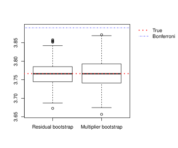
Figure 16: Boxplots comparing the estimates of the multiplier bootstrap and the residual bootstrap for the 95% quantile of the distribution $\max_{j\in\{1,\dots,p\}}|T_{j}|\>\>\>\mbox{under}\>\>\>H_{0,\mathrm{complete}}$. The boxplots are based on 500 estimates, each computed for a different realization of the model. The dimensions are $n=100,\ p=500$ for a matrix of Toeplitz design type. The errors are homoscedastic Gaussian $\varepsilon\sim\mathcal{N}_{n}(0,I_{n})$. The horizontal red line denotes the true value of the quantile, the blue line denotes the corresponding Bonferroni rejection threshold.

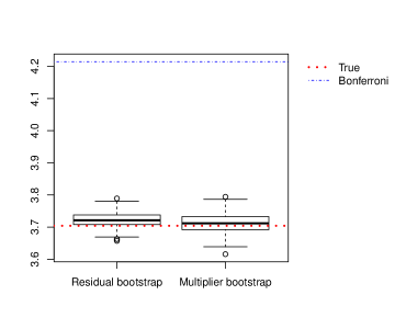
Figure 17: Boxplots comparing the estimates of the multiplier bootstrap and the residual bootstrap for the 95% quantile of the distribution $\max_{j\in\{1,\dots,p\}}|T_{j}|\>\>\>\mbox{under}\>\>\>H_{0,\mathrm{complete}}$. The boxplots are based on 500 estimates, each computed for a different realization of the model. The dimensions are $n=30,p=2000$ for a matrix of Toeplitz design type. The errors are homoscedastic chi-squared as described in Section 5.1.2. The horizontal red line denotes the true value of the quantile, the blue line denotes the corresponding Bonferroni rejection threshold.

Next, we compare the robust version of the test statistic $T_{j}=\hat{b}_{j}/\widehat{s.e.}_{\mathrm{robust},j}$ to the one with non-robust studentization, for both the bootstrap approaches. In Figure 18 the comparison of the residual bootstrap methods can be found for the homoscedastic linear model used in Figure 16. Figure 19 compares both versions of the multiplier bootstrap for heteroscedastic errors (taken from Section 5.1.3), with a design matrix of type Toeplitz of dimensions $n=30,p=2000$. The robust version of the bootstrap performs well in the heteroscedastic example. For the homoscedastic case, the Bootstrap for the robust test-statistic doesn’t seem to gain over Bonferroni.

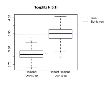
Figure 18: Same as Figure 16 but comparing the estimates of the non-robust studentized estimator to the robust version. Due to the difference in the test statistics, the underlying true quantiles are different. The residual bootstrap is used.

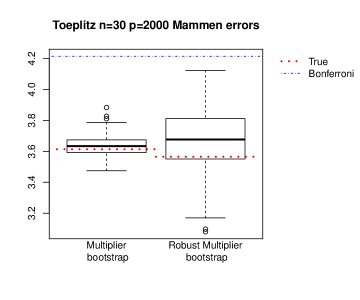
Figure 19: Same as Figure 18, but for a Toeplitz design matrix of different dimensions ($n=30,p=2000$) and with heteroscedastic errors as described in Section 5.1.3. The multiplier bootstrap is used for the estimator with either the robust or non-robust studentization. The Gaussian multiplier wild bootstrap is used (the non-robust studentization does not lead to $N(0,1)$ scaling of the components in the maximum).

A.4.2 All results for the multiplier bootstrap

We compare the residual bootstrap approach to the wild bootstrap for all the results from Section 5.1.

For the homoscedastic Gaussian errors, the confidence intervals comparison can be found in Figures 20 and 21, the multiple testing results can be found in Figure 22. For the homoscedastic non-Gaussian errors, the confidence intervals comparison can be found in Figures 23 and 24, the multiple testing results can be found in Figure 25. For the heteroscedastic non-Gaussian errors, the confidence intervals comparison can be found in Figures 26 and 27, the multiple testing results can be found in Figure 28.

The differences in performance seem very minimal. The wild bootstrap has no problem dealing with heteroscedastic errors, it performs similar to the robust bootstrap approach in our example.

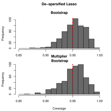
Figure 20: Same plot as the homoscedastic Gaussian results in Figure 4, but showing also the multiplier bootstrap.

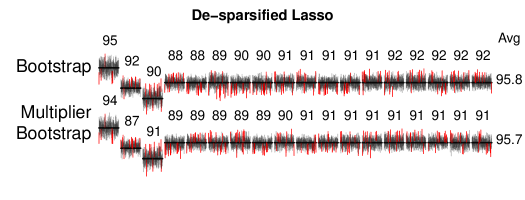
Figure 21: Same plot as the homoscedastic Gaussian results in Figure 5, but showing also the multiplier bootstrap.

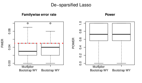
Figure 22: Same plot as the homoscedastic Gaussian results in Figure 6, but showing also the multiplier bootstrap.

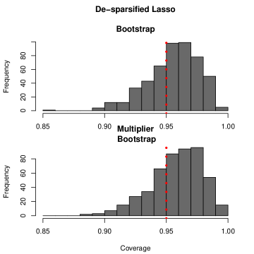
Figure 23: The same plot as Figure 4 but for homoscedastic chi-squared errors and showing also the multiplier bootstrap.

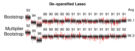
Figure 24: The same plot as Figure 5 but for homoscedastic chi-squared errors and showing also the multiplier bootstrap.

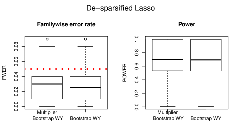
Figure 25: The same plot as Figure 6 but for homoscedastic chi-squared errors and showing also the multiplier bootstrap.

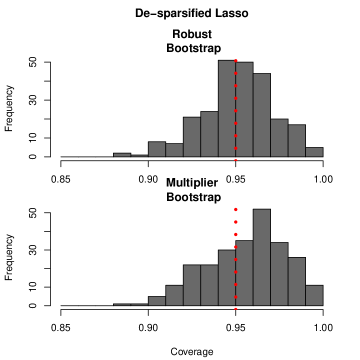
Figure 26: The same plot as Figure 4 but for heteroscedastic non-Gaussian errors and showing also the multiplier bootstrap (the latter with non-robust studentization).

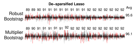
Figure 27: The same plot as Figure 5 but for heteroscedastic non-Gaussian errors and showing also the multiplier bootstrap (the latter with non-robust studentization).

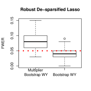
Figure 28: The same plot as Figure 6 but for heteroscedastic non-Gaussian errors with robust studentization and showing also the multiplier bootstrap.

A.4.3 Homoscedastic non-Gaussian errors - Robust estimators

We present in Figures 29 and 30 some results about individual inference when using the robust studentization in presence of homoscedastic errors: an efficiency loss is not really visible.

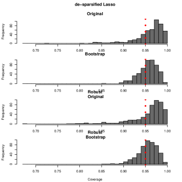
Figure 29: The same plot as Figure 7 with homoscedastic chi-squared errors but also including the robust alternatives of the estimators.

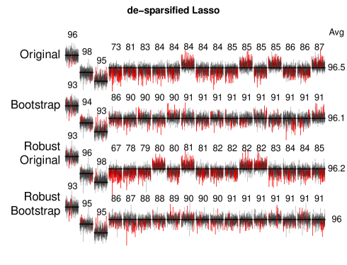
Figure 30: The same plot as Figure 8 with homoscedastic chi-squared errors but also including the robust alternatives of the estimators. The original estimator (both robust and non robust) has quite some bias for a few coefficients, which results in a lower than desired coverage for those coefficients.

References

- Bickel et al., (1998) Bickel, P., Klaassen, C., Ritov, Y., and Wellner, J. (1998). Efficient and Adaptive Estimation for Semiparametric Models. Springer.
- Breiman, (1996) Breiman, L. (1996). Heuristics of instability and stabilization in model selection. Annals of Statistics, 24:2350–2383.
- Bühlmann, (2013) Bühlmann, P. (2013). Statistical significance in high-dimensional linear models. Bernoulli, 19:1212–1242.
- Bühlmann et al., (2014) Bühlmann, P., Kalisch, M., and Meier, L. (2014). High-dimensional statistics with a view towards applications in biology. Annual Review of Statistics and its Applications, 1:255–278.
- Bühlmann and van de Geer, (2011) Bühlmann, P. and van de Geer, S. (2011). Statistics for High-Dimensional Data: Methods, Theory and Applications. Springer.
- Bühlmann and van de Geer, (2015) Bühlmann, P. and van de Geer, S. (2015). High-dimensional inference in misspecified linear models. Electronic Journal of Statistics, 9:1449–1473.
- Chatterjee and Lahiri, (2011) Chatterjee, A. and Lahiri, S. (2011). Bootstrapping Lasso estimators. Journal of the American Statistical Association, 106:608–625.
- Chatterjee and Lahiri, (2013) Chatterjee, A. and Lahiri, S. (2013). Rates of convergence of the adaptive LASSO estimators to the oracle distribution and higher order refinements by the bootstrap. Annals of Statistics, 41:1232–1259.
- Chernozhukov et al., (2013) Chernozhukov, V., Chetverikov, D., and Kato, K. (2013). Gaussian approximations and multiplier bootstrap for maxima of sums of high-dimensional random vectors. Annals of Statistics, 41:2786–2819.
- Dezeure et al., (2015) Dezeure, R., Bühlmann, P., Meier, L., and Meinshausen, N. (2015). High-dimensional inference: Confidence intervals, -values and R-software hdi. Statistical Science, 30:533–558.
- Efron, (1979) Efron, B. (1979). Bootstrap methods: Another look at the jackknife. Annals of Statistics, 7:1–26.
- Eicker, (1967) Eicker, F. (1967). Limit theorems for regressions with unequal and dependent errors. In Proceedings of the fifth Berkeley symposium on mathematical statistics and probability, volume 1, pages 59–82.
- Foygel Barber and Candès, (2015) Foygel Barber, R. and Candès, E. J. (2015). Controlling the false discovery rate via knockoffs. Annals of Statistics, 43:2055–2085.
- Freedman, (1981) Freedman, D. A. (1981). Bootstrapping regression models. Annals of Statistics, 9:1218–1228.
- Gine and Zinn, (1989) Gine, E. and Zinn, J. (1989). Necessary conditions for the bootstrap of the mean. Annals of Statistics, 17:684–691.
- Gine and Zinn, (1990) Gine, E. and Zinn, J. (1990). Bootstrapping general empirical measures. Annals of Probability, 18:851–869.
- Hall and Wilson, (1991) Hall, P. and Wilson, S. R. (1991). Two guidelines for bootstrap hypothesis testing. Biometrics, 47:pp. 757–762.
- Huber, (1967) Huber, P. J. (1967). The behavior of maximum likelihood estimates under nonstandard conditions. In Proceedings of the fifth Berkeley symposium on mathematical statistics and probability, volume 1, pages 221–233.
- Javanmard and Montanari, (2014) Javanmard, A. and Montanari, A. (2014). Confidence intervals and hypothesis testing for high-dimensional regression. Journal of Machine Learning Research, 15:2869–2909.
- Liu and Singh, (1992) Liu, R. Y. and Singh, K. (1992). Efficiency and robustness in resampling. Annals of Statistics, 20:370–384.
- Mammen, (1993) Mammen, E. (1993). Bootstrap and wild bootstrap for high dimensional linear models. Annals of Statistics, 21:255–285.
- McKeague and Qian, (2015) McKeague, I. W. and Qian, M. (2015). An Adaptive Resampling Test for Detecting the Presence of Significant Predictors. Journal of the American Statistical Association, 110:1422–1433.
- Meier et al., (2016) Meier, L., Dezeure, R., Meinshausen, N., Mächler, M., and Bühlmann, P. (2016). hdi: High-Dimensional Inference. R package version 0.1-6.
- Meinshausen, (2015) Meinshausen, N. (2015). Group bound: confidence intervals for groups of variables in sparse high dimensional regression without assumptions on the design. Journal of the Royal Statistical Society, Series B, 77:923–945.
- Meinshausen and Bühlmann, (2006) Meinshausen, N. and Bühlmann, P. (2006). High-dimensional graphs and variable selection with the Lasso. Annals of Statistics, 34:1436–1462.
- Meinshausen and Bühlmann, (2010) Meinshausen, N. and Bühlmann, P. (2010). Stability Selection (with discussion). Journal of the Royal Statistical Society, Series B, 72:417–473.
- Meinshausen et al., (2011) Meinshausen, N., Maathuis, M. H., and Bühlmann, P. (2011). Asymptotic optimality of the Westfall-Young permutation procedure for multiple testing under dependence. Annals of Statistics, 39:3369–3391.
- Meinshausen et al., (2009) Meinshausen, N., Meier, L., and Bühlmann, P. (2009). P-values for high-dimensional regression. Journal of the American Statistical Association, 104:1671–1681.
- Reid et al., (2016) Reid, S., Tibshirani, R., and Friedman, J. (2016). A study of error variance estimation in lasso regression. Statistica Sinica, 26:35–67.
- Rudelson and Zhou, (2013) Rudelson, M. and Zhou, S. (2013). Reconstruction from anisotropic random measurements. Information Theory, IEEE Transactions on, 59:3434–3447.
- Shah and Bühlmann, (2015) Shah, R. and Bühlmann, P. (2015). Goodness of fit tests for high-dimensional models. Preprint arXiv:1511.03334.
- Shah and Samworth, (2013) Shah, R. and Samworth, R. (2013). Variable selection with error control: another look at Stability Selection. Journal of the Royal Statistical Society Series B, 75:55–80.
- van de Geer et al., (2014) van de Geer, S., Bühlmann, P., Ritov, Y., and Dezeure, R. (2014). On asymptotically optimal confidence regions and tests for high-dimensional models. Annals of Statistics, 42:1166–1202.
- van de Geer et al., (2011) van de Geer, S., Bühlmann, P., and Zhou, S. (2011). The adaptive and the thresholded Lasso for potentially misspecified models (and a lower bound for the Lasso). Electronic Journal of Statistics, 5:688–749.
- Wasserman and Roeder, (2009) Wasserman, L. and Roeder, K. (2009). High dimensional variable selection. Annals of Statistics, 37:2178–2201.
- Westfall and Young, (1993) Westfall, P. and Young, S. (1993). Resampling-based Multiple Testing: Examples and Methods for P-value Adjustment. John Wiley & Sons.
- White, (1980) White, H. (1980). A heteroskedasticity-consistent covariance matrix estimator and a direct test for heteroskedasticity. Econometrica, 48:817–838.
- Wu, (1986) Wu, C.-F. J. (1986). Jackknife, bootstrap and other resampling methods in regression analysis. Annals of Statistics, 14:1261–1295.
- Ye and Zhang, (2010) Ye, F. and Zhang, C.-H. (2010). Rate minimaxity of the Lasso and Dantzig selector for the loss in balls. Journal of Machine Learning Research, 11:3481–3502.
- Zhang and Huang, (2008) Zhang, C.-H. and Huang, J. (2008). The sparsity and bias of the Lasso selection in high-dimensional linear regression. Annals of Statistics, 36:1567–1594.
- Zhang and Zhang, (2014) Zhang, C.-H. and Zhang, S. S. (2014). Confidence intervals for low dimensional parameters in high dimensional linear models. Journal of the Royal Statistical Society, Series B, 76:217–242.
- Zhang and Cheng, (2016) Zhang, X. and Cheng, G. (2016). Simultaneous inference for high-dimensional linear models. Journal of the American Statistical Association. Published online, DOI:10.1080/01621459.2016.1166114.
- Zhou, (2014) Zhou, Q. (2014). Monte Carlo Simulation for Lasso-Type Problems by Estimator Augmentation. Journal of the American Statistical Association, 109:1495–1516.