Does the velocity of light depend on the source movement?

Abstract

Data from spacecrafts tracking exhibit many anomalies that suggest the dependence of the speed of electromagnetic radiation with the motion of its source. This dependence is different from that predicted from emission theories that long ago have been demonstrated to be wrong. By relating the velocity of light and the corresponding Doppler effect with the velocity of the source at the time of detection, instead of the time of emission, it is possible to explain quantitatively and qualitatively the spacecraft anomalies. Also, a formulation of electromagnetism compatible with this conception is possible (and also compatible with the known electromagnetic phenomena). Under this theory the influence of the velocity of the source in the speed of light is somewhat subtle in many practical situations and probably went unnoticed in other phenomena.

I Introduction

In these lines I intend to show that there exists consistent evidence pointing to the need of revision and further study of what seem at present a settled issue, namely the independence of the speed of electromagnetic radiation on the motion of its source.

The main point in the evidence is the range disagreement during the Earth flyby of the spacecraft NEAR in 1998. Its range was measured near the point of closest approach using two radar stations of the Space Surveillance Network (SSN), and compared with the trajectory obtained from the Deep Space Network (DSN)antreasian98 . As for the range, the two measurements should match within a meter-level accuracy (the resolution is 5 m for Millstone and 25 m for Altair), but actual data showed a difference that varies linearly with time (with different slopes for the two radar stations) up to a maximum difference of about 1 km, i.e. more than 100 times larger than the accuracy of the equipment used (see figure 10 of antreasian98 ). Further, when NEAR crossed the orbits of GPS satellites (orbital radius 26,600 Km) the measured range difference was 650 m, that is, a time difference of 2 $\mu$s. Is it reasonable that any standard GPS receiver performs better than DSN or SSN?

There has not been a complete explanation for the range discrepancy. It is very difficult to find any physical reason that may produce this anomaly, for any physical disturbance of the path of the spacecraft should manifest equally in SSN and DSN measurements. Guruprasadchirp proposed an explanation that points to a time lag in the DSN signals, but the model is, at best, within 10% of the measured data and, more important, it fails to explain an important feature, that is, the different slope for the two radars. If we assume that systems are working properly, then the measured range difference (time lag) could be due to different propagation time of the employed signals.

Additional points in the evidence come from anomalies related to the tracking of spacecrafts, present in both Doppler and ranging data. The Pioneer anomalyanderson98 and the flyby anomalyanderson08 refer to small residuals of the differences between measured and modeled Doppler frequencies of the radio signals emitted by the spacecrafts. Although these residuals are very small (less than 1 Hz on GHz signals) the problem is that they follow a non-random pattern, indicating failures of the model. According to the temporal variation of those residuals the Pioneer anomaly exhibits a main term, an annual term, a diurnal term and a term that appears during planetary encounters. It should be clarified that a few years ago an explanation of the Pioneer anomaly was publishedturyshev12 . However, it is a very specific solution that applies only to the main term of the Pioneer spacecraft anomaly, but left unresolved many other anomalies, including those of the spaceships Cassini, Ulysses and Galileo; the annual term; the diurnal term; the increases of the anomaly during planetary encounters; the flyby anomaly; and the possible link between all them (it is hard to think that there are so many different causes for the mentioned anomalies). For all this, I believe that the issue can not be closed as it stands.

II Range disagreement

As a matter of fact, the range difference between SSN and DSN, $\delta R$, is perfectly fitted with

$$\delta R\left(t\right)=-\frac{{\bf R}\left(t\right)\cdot{\bf v}\left(t\right)}{c}$$ (1)

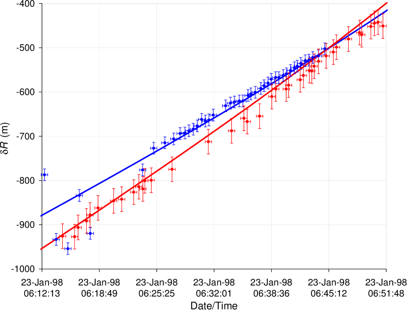
Figure 1: Range disagreement between SSN and DSN, for 1998 NEAR flyby (Millstone blue points, upper trace, and Altair red points, lower trace). Also the fit (1) is plotted (full lines, Millstone in blue and Altair in red). For Millstone, the error bars refer to the uncertainties in the extraction of the data from figure 10 of antreasian98 , rather than to its tracking error (5 m), while for Altair, the accuracy is 25 m

where ${\bf R}\left(t\right)$ is a vector range pointing from the spacecraft to the radar, ${\bf v}\left(t\right)$ the spacecraft velocity relative to the radar, and $c$ the speed of light. Figure 1 shows this fit and its comparison with measured data. The orbital and measured data were taken fromantreasian98 . Although the exact location of the radar stations are unknown, the fit is statistically significant for both radar stations ($p<10^{-3}$) including the first outliers points. It reproduces the (almost) linear dependence with time during the measured interval, and the two different slopes for Millstone and Altair stations due to their different locations.

Since range measurements are based on time-of-flight techniques, the validity of (1) means that the electromagnetic waves (microwave) of the DSN and SSN travel at different speeds. Specifically, in the radar frame of reference, if the SSN waves travel at $c$, then the DSN waves travel at $c$ plus the projection of the spacecraft velocity in the direction of the beam, in sharp contrast with the Second Postulate of Special Relativity Theory (SRT).

In view of the above result one may ask what is established, at present, about the relation of the speed of electromagnetic radiation (light for short) to the motion of the source. In order to elaborate this point the following questions are of relevance:

1. Are there simultaneous measurements of the speed of light from different moving macroscopic sources (not moving images) with different velocities?;

2. Since ballistic (emission) theories are ruled out (see, for example, DeSitter desitter13a desitter13b , Brecher brecher77 and Alvager et al alvager64 ), how else could the speed of light depend on the source movement?

3. How is it possible that there is a first order difference in $v/c$ in spacecraft range measurements, while at the same time there are many experiments on time dilation that are consistent with SRT to second order in $v/c$ (see, for example,boterman14 )?;

4. If the velocity of light depend on the velocity of the source, why has this not been observed in other phenomena in the past?;

In answer to the previous questions, so far as the author is aware, there is no known experimental work that simultaneously measures the speed of light from two different sources (not images), or that simultaneously measures the speed of light and that of its source. For example, in the work by Alvager et al,alvager64 the speed of light is measured at a later time ($\approx$ 200 ns) than the emission time, and there is no measurement of the speed of the source at the time of the detection of the light.

Note that measurements involving moving images produce different results from those produced by mobile sources. For example, under SRT, a moving source is affected by time dilation while a moving image is not. Therefore, to ensure the independence of the speed of light from its source movement, it is essential to have two sources with different movements.

Although controversial and beyond the scope of the this note, time dilatation phenomena may be of different physical origin from first order terms, as it may be inferred from the work of Schrödinger schrodinger25 . Thus, measurements of time dilatation phenomena in accordance with SRT, does not necessarily imply the independence of the speed of light with the movement of the source.

The experiments mentioned above desitter13a desitter13b brecher77 alvager64 only rule out ballistic theories in which radiation maintains the speed of the source at the time of emission, but do not rule out other ideas, like Faraday’s 1846faraday46 .

III Faraday’s ray vibrations

In order to remove the ether, Faraday introduced the concept of vibrating raysfaraday46 , in which an electric charge is conceived as a center of force with attached “rays” that extend to infinity. The rays move with their center, but without rotating. According to this view, the phenomenon of electromagnetic radiation corresponds to the vibration of these “rays,” that propagates at speed $c$ relative to the rays (and the center). That is, the radiation remains linked to the source even after emitted. Today we could describe the interaction as a kind of entanglement between the charge and the photon. A framework for the electromagnetic phenomena according to Faraday’s ideas was developed. It was called “Vibrating Rays Theory” (VRT) bilbao14 in reference to Faraday’s “vibrating rays.”

Under Faraday’s idea, the velocity of radiation at a given epoch will be equal to c plus the velocity of the source at the same epoch, in contrast with ballistic theories in which the emitted light retains the speed of the source at the emission epoch. In this sense the radiation is always linked to the charge at every time after the emission. Consequently, the measured Doppler Effect corresponds to the speed of the source at the time of reception, as well.

Further, a difference between active and passive reflection is expected, since the latter is still related to the original source according to VRT. The Deep Space Network (DSN) works with the so called active reflection (the spacecraft re-emits in real time a signal in phase with the received signal from Earth), while the Space Surveillance Network (SSN) works with passive radar reflection. In consequence, the downlink signal from the aproaching spacecraft will propagate faster that the reflected one. Using the available orbital dataantreasian98 we found that, under VRT, the theoretical time-of-flight difference between active and passive reflection gives exactly the same range disagreement as (1), see Part 6 of bilbao14 .

IV Pioneer anomaly

The Pioneer anomaly refers to the fact that the received Doppler frequency differs from the modeled one by a blue shift that varies almost linearly with time, and whose derivative is

$$\frac{d(\Delta f)}{dt}\approx-6\times 10^{-9}\text{ Hz}/\text{s}$$ (2)

where $\Delta f$ is the frequency difference between the measured and the modeled values.

In the case of a source with variable speed, the main difference in Doppler (to first order) between VRT and SRT, is that SRT relates to the speed of the source at the time of emission, while VRT relates to the speed of the source at the time of reception. Precisely, this difference seems to be present in the spacecraft anomalies.

If VRT is valid, it automatically invalidates all calculations and data analysis of spacecraft tracking which are based on SRT. So, it is not easy to make a direct comparison between the expected results from SRT and VRT. However, to see whether or not the main features predicted by VRT are present in the measurements, we can evaluate the residual by simulating a measured Doppler signal assuming that light propagates in accordance to VRT but analyzed according to SRT.

Calling $t_{2}$ the emission time of the downlink signal from the spacecraft toward Earth and $t_{3}$ the reception time at Earth, the first order difference of the Doppler shift between VRT and SRT is (see bilbao14 Part 4)

$$\Delta f=f_{VRT}-f_{SRT}\approx f_{0}\hat{{\bf r}}\cdot\frac{{\bf v}_{2}-{\bf v}_{3}}{c}$$ (3)

where ${\bf v}_{2}$ and ${\bf v}_{3}$ represent the velocities of the spacecraft at the corresponding epoch, $\hat{{\bf r}}$ is the unit vector from the spacecraft to the antenna, and $f_{0}$ the proper frequency of the signal. That is, the velocity used in the SRT formula is that at the time of emission while according to VRT is that corresponding at the time of reception.

Since the spacecraft slows down as it moves away, then $\hat{{\bf r}}\cdot\left({\bf v}_{2}-{\bf v}_{3}\right)>0$, therefore the difference corresponds to a small blue shift mounted over the large red shift, as it has been observed in the Pioneer anomaly. It should be noted that this difference appears because of the active reflection produced by the onboard transmitter. In case of a passive reflection (for example, by means of a mirror) the above difference vanishes.

IV.1 Main term

An estimate of the order of magnitude of 3 is obtained by using that the variation of the velocity of the spacecraft between the time of emission and reception is approximately

$${\bf v}_{2}-{\bf v}_{3}\approx{\bf a}\left(t_{2}-t_{3}\right)$$ (4)

where ${\bf a}$ is a mean acceleration during the downlink interval. An estimate for the duration of the downlink is simply

$$t_{3}-t_{2}\approx\frac{r}{c}$$ (5)

where $r$ is a mean position of the spacecraft between $t_{2}$ and $t_{3}$, therefore

$$\Delta f\approx-f_{0}\frac{{\bf r}\cdot{\bf a}}{c^{2}}$$

Since

$${\bf a=-}\frac{GM}{r^{2}}\hat{{\bf r}}$$

where $G$ is the gravitational constant, and $M$ the mass of the Sun, then, the time derivative becomes

$$\frac{d\left(\Delta f\right)}{dt}\approx f_{0}\frac{{\bf v}\cdot{\bf a}}{c^{2}}$$ (6)

If the difference (6) is interpreted as an anomalous acceleration we get

$$a_{a}\approx\frac{v}{c}a$$ (7)

that is, the so-called anomalous acceleration is $v/c$ times the actual acceleration of the spacecraft.

Using data from HORIZONS Web-Interface nasa for the spacecraft ephemeris, some characteristic value for $a_{a}$ can be obtained. Consider the anomalous acceleration detected at the shortest distance of the Cassini spacecraft during solar conjunction in June, 2002. The spacecraft was at a distance of $7.42$ AU moving at a speed of $5.76$ km/s. The anomalous acceleration given by (7) is $a_{a}\approx 2\times 10^{-9}$ m/s² of the same order of the measured one ($\approx 2.7\times 10^{-9}$ m/s² ). Also, the closest distance at which the Pioneer anomaly has been detected was about $20$ AU. the anomalous acceleration predicted by (7) at that distance is $a_{a}\approx 7.3\times 10^{-10}$ m/s² of the same order as the measured one.

The “anomaly” given by (7) decreases in time in a way that has not been observed. Note, however, that according to Markwardt markwardt02 the expected frequency at the receiver includes an additional Doppler effect caused by small effective path length changes, given by

$$\Delta f_{path}=-\frac{2f_{0}}{c}\frac{dl}{dt}$$ (8)

where $dl/dt$ is the rate of change of effective photon trajectory path length along the line of sight. This is a first order effect that can partially hide the difference between SRT and VRT. Therefore, a more careful analysis should take into account the additional contribution of (8) in (7).

Further, other first order effects may appear, for example, by a slight rotation of the orbital plane. Since orbital parameters are obtained by periodically fitting the measurements (mainly due to spacecraft maneuvers or random perturbations) with theoretical orbits, there is no straightforward way to weight the importance of this effect in (7). In other words, data acquisition and analysis may hide part of the VRT signature.

IV.2 Annual term

Apart from the residual referred to in the preceding paragraph there is also an annual term. According to Anderson et al anderson02 the problem is due to modeling errors of the parameters that determine the spacecraft orientation with respect to the reference system. Anyway, Levy et al levy08 claim that errors such as errors in the Earth ephemeris, the orientation of the Earth spin axis or the stations coordinates are strongly constrained by other observational methods and it seems difficult to modify them sufficiently to explain the periodic anomaly.

The advantage of studying the annual term over the main term, is that the former is less sensitive to the first order correction mentioned above, and, for the case of Pioneer, also to the thermal propulsion correctionturyshev12 . Clearly, the Earth orbital position does not modify those terms.

As before, the annual term is explained by the difference between the velocity of the spacecraft at the time of emission and that at the moment of detection, which depends on whether the spacecraft is in opposition or in conjunction relative to the Sun. When the spacecraft is in conjunction, light takes longer to get back to Earth than in opposition. The time difference between emission and reception will be increased by the time the light takes in crossing the Earth orbit. Specifically, taking into account the delay due to the position of Earth in its orbit, in opposition equation (5) should be written as

$$t_{3}-t_{2}\approx\frac{r+R_{orb}}{c}$$ (9)

while in conjunction it would be

$$t_{3}-t_{2}\approx\frac{r-R_{orb}}{c}$$ (10)

where $R_{orb}$ is the mean orbital radius of Earth.

Therefore, an estimate of the magnitude of the amplitude of the annual term is

$$\Delta f\approx f_{0}\frac{aR_{orb}}{c^{2}}$$ (11)

For the case of Pioneer 10 at 40 AU we get

$$\Delta f\approx 14\text{ mHz}$$ (12)

and at 69 AU

$$\Delta f\approx 4.8\text{ mHz}$$ (13)

in good agreement with the observed values.

Using data from HORIZONS Web-Interface nasa a more complete analysis of the time variation of $\Delta f$ has be performed. The residual (that is, simulated Doppler using VRT but interpreted under SRT) during 12 years time span is plotted in figure 2. Also the dumped sine best fit of the 50 days average measured by Turyshev et al turyshev99 is plotted showing an excellent agreement between measurements and VRT prediction. The negative peaks (i.e., maximum anomalous acceleration) occur during conjunction when the Earth is further apart from the spacecraft, and positive peaks during opposition. Also, the amplitude is larger at the beginning of the plotted interval and decreases with time, as it was observedanderson08 turyshev99 .

V Flyby anomaly

Like the Pioneer anomaly, the Earth flyby anomaly can be associated to a modeling problem, in the sense that relativistic Doppler includes terms that are absent in the measured signals. The empirical equation of the flyby anomaly is given by Anderson et alanderson08 , which, notably, can be derived using VRT, as is done in Part 6 of bilbao14 .

Consider the case of NEAR tracked by 3 antennas located in USA, Spain, and Australia (a full description of the tracking system is found in a series of monographs of the Jet Propulsion Laboratorydescanso ). The receiving antenna was chosen as that having a minimum angle between the spacecraft and the local zenith.

Using available orbital data, a simulated Doppler signal has been calculated using VRT. Thus, the simulated residual is obtained by subtracting the theoretical SRT Doppler, from the VRT calculation. We observed, however, that the term that contains the velocity of the antennas, that is

$$d=\frac{\gamma_{u_{3}}}{\gamma_{u_{1}}}\frac{1-\hat{{\bf r}}_{23}\cdot{\bf u}_{3}/c}{1-\hat{{\bf r}}_{12}\cdot{\bf u}_{1}/c}$$ (14)

is not enough to completely remove the first order (in $u/c$) Earth signature (${\bf u}$ is the velocity of the antenna, 1 refers to the emission epoch and 3 to the reception epoch, as in bilbao14 Part 4).

This is so because the velocity of the antennas is not uniform and the evaluation of the emission time is different for VRT and SRT. Then, a small, first order related term remains. Anyway, since orbital parameters are obtained by periodically fitting the measurements to theoretical orbits, thus a similar procedure is needed for VRT. By doing so the first order term is removed. The only difference between orbits adjusted by SRT and VRT is a slight rotation of the orbit plane, as mentioned above. Note that, in the case of range disagreement, two different orbital ajustment are needed by DSN and SSN due to the different propagation speed. In consequence, it will be impossible to fit a simultaneous measurement, as it seems to happen with the range disagreement.

The final result shows that each antenna produces a sinusoidal residual with a phase shift at the moment of maximum approach. Therefore, if we fit the data with the pre-encounter sinusoid a post-encounter residual remains and vice versa.

In figure 3 are simultaneously plotted the result of fitting the residual by pre-encounter data (right half in red, corresponding to figure 2a of anderson08 ) and by post-encounter data (left half in blue, corresponding to figure 2b of anderson08 ).

Note that the simulated plots are remarkably similar to the reported ones, including the amplitude and phase (i.e., minima and maxima) of the corresponding antenna. The fitting of post-encounter data (blue) can be improved by appropriately setting the exact switching times of the antennas (which are unknown to the author). The flyby Doppler residual exhibits a clean signature of the VRT theory.

VI Conclusions

In this work I have presented observational evidence favoring a dependence of the speed of light on that of the source, in the manner implied in Faraday’s ideas of “vibrating rays.”

It is remarkable and very suggestive that, as derived from Faraday’s thoughts, simply by relating the velocity of light and the corresponding Doppler effect with the velocity of the source at the time of detection, is enough to quantitatively and qualitatively explain a variety of spacecraft anomalies.

Also, it is worth mentioning that a formulation of electromagnetism compatible with Faraday’s conception is possible, as shown in bilbao14 , which is also compatible with the known electromagnetic phenomena. This new formalism introduces a striking concept: that both instantaneous interaction (static terms) and retarded interaction (radiative terms) are simultaneously present.

Finally, under VRT the manifestation of the movement of the source in the speed of light is more subtle than the naive $c+kv$ hypothesis ($k$ is a constant, $0\leq k\leq 1$) usually used to test their dependencebrecher77 . Thus, it is also of fundamental importance the fact that, from the experimental point of view, it is very difficult to detect differences between VRT and SRT, as discussed in bilbao14 , which is also manifest in the smallness of the measured anomalies, and in the non clear manifestation of the effect in usual experiments and observations. For example, it produces a negligible effect on satellite positioning systems, see Part 7 ofbilbao14 .

I am aware of how counterintuitive these conceptions are to the modern scientist, but also believe that, given the above evidence, a conscientious experimental research is needed to settle the question of the dependence of the speed of light on that of its source as predicted by VRT, and that has been observed during the 1998 NEAR flyby. As a closure, I recall Fox’s words regarding the possibility of conducting an experiment on the propagation of light relative to the motion of the source: “Nevertheless if one balances the overwhelming odds against such an experiment yielding anything new against the overwhelming importance of the point to be tested, he may conclude that the experiment should be performed.” fox62

VII Figures

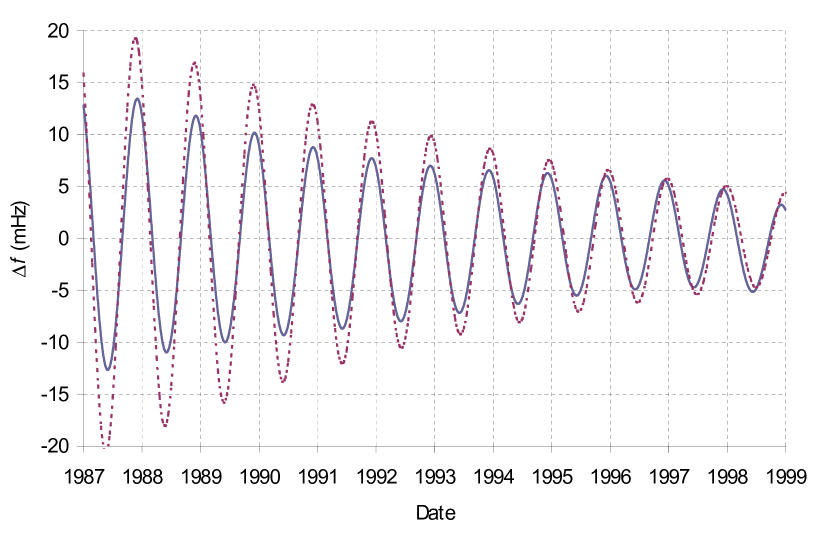
Figure 2: Annual variation of the frequency difference between VRT and SRT (full line) and anomalous dumped sine best fit of the 50 days average measured by Turyshev et al turyshev99 (dashed line), for Pioneer 10 from January 1987 to January 1999.

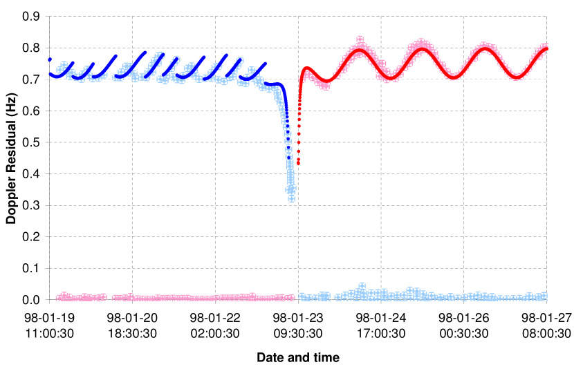
Figure 3: Fitting the pre- (right half, in red) and post-encounter (left half, in blue) X-band Doppler data residual, for the NEAR flyby under an ideal hyperbolic orbit. Solid lines simulated according to VRT. Crosses, actual data extracted from reference anderson08 .

References

- (1) P. G. Antreasian and J. R. Guinn, AIAA Paper No. 98-4287 presented at the AIAA/AAS Astrodynamics Specialist Conference and Exhibit (Boston, August 10-12, 1998).
- (2) V. Guruprasad, EPL 110, 54001 (2015).
- (3) J. D. Anderson, P. A. Laing, E. L. Lau, A. S. Liu, M. M. Nieto, and S. G. Turyshev, Phys. Rev. Lett. 81, 2858-2861 (1998).
- (4) J. D. Anderson, J. K. Campbell, J. E. Ekelund, J. Ellis, and J. F. Jordan, Phys. Rev. Lett. 100, 091102 (2008).
- (5) S. G. Turyshev, V. T. Toth, G. Kinsella, S.-C. Lee, S. M. Lok, and J. Ellis, Phys. Rev. Lett. 108, 241101 (2012)
- (6) W. deSitter, Z. Phys. 14, 429 (1913).
- (7) W. deSitter, Z. Phys. 14, 1267 (1913).
- (8) K. Brecher, Phys. Rev. Lett. 39, 1051 (1977).
- (9) T. Alvager, F. J. M. Farley, J. Kjellman, and I. Wallin, Phys. Lett. 12, 260 (1964).
- (10) B. Botermann et al, Phys. Rev. Lett. 113, 120405 (2014).
- (11) E. Schrodinger; Ann. der Physik 77, 325-336 (1925).
- (12) M. Faraday, Phil. Mag. 28, 345 (1846).
- (13) L. Bilbao, L. Bernal, F. Minotti; “Vibrating Rays Theory,” arXiv:1407.5001 [physics.class-ph] (2014).
- (14) http://ssd.jpl.nasa.gov/.
- (15) C. B. Markwardt, “Independent Confirmation of the Pioneer 10 Anomalous Acceleration,” arXiv:gr-qc/0208046 v1 (2002).
- (16) J. D. Anderson, P. A. Laing, E. L. Lau, A. S. Liu, M. M. Nieto, and S. G. Turyshev, Phys. Rev. D 65, 082004 (2002).
- (17) A. Levy, B. Christophe, S. Reynaud, J-M. Courty, P. Brio, and G. Mtris, “Pioneer 10 data analysis: investigation on periodic anomalies,” in Journées scientifiques de la SF2A, Paris, France pp.133-136, 2008. «hal-00417743»
- (18) G. Turyshev et al, arXiv:gr-qc/9903024 v2 (1999).
- (19) DESCANSOTeam, Jet Propulsion Laboratory, California Institute of Technology. http://descanso.jpl.nasa.gov/Monograph/mono.cfm (accessed July 2014).
- (20) J. G. Fox, Am. J. Phys. 30, 297 (1962).