Small Cell Offloading Through Cooperative Communication in Software-Defined Heterogeneous Networks

Abstract

To meet the ever-growing demand for a higher communicating rate and better communication quality, more and more small cells are overlaid under the macro base station (MBS) tier, thus forming the heterogeneous networks. Small cells can ease the load pressure of MBS but lack of the guarantee of performance. On the other hand, cooperation draws more and more attention because of the great potential of small cell densification. Some technologies matured in wired network can also be applied to cellular networks, such as Software-defined networking (SDN). SDN helps simplify the structure of multi-tier networks. And it’s more reasonable for the SDN controller to implement cell coordination. In this paper, we propose a method to offload users from MBSs through small cell cooperation in heterogeneous networks. Association probability is the main indicator of offloading. By using the tools from stochastic geometry, we then obtain the coverage probabilities when users are associated with different types of base stations (BSs). All the cell association and cooperation are conducted by the SDN controller. Then on this basis, we compare the overall coverage probabilities, achievable rate and energy efficiency with and without cooperation. Numerical results show that small cell cooperation can offload more users from MBS tier. It can also increase the system’s coverage performance. As small cells become denser, cooperation can bring more gains to the energy efficiency of the network.

I Introduction

Along with the huge increasing of mobile users, the current wireless communication system is facing with the great challenges of system capacity and quality-of-service (QoS) requirements [1]. 5G is expected to achieve gigabit-level throughput and more varied service capabilities in an energy-efficient way by 2020 [2, 3]. In [4] and [5], mobile cloud and wearable computing is implemented in 5G to improve Quality of Experience (QoE) and overcome the energy bottleneck. The deployment of small cells seems to be one of the most feasible solutions for the areas with a large traffic demand. Heterogeneous networks (HetNets) where macro and small cells coexist have been widely applied [6]. BSs in different tiers differ in transmit power, coverage range, and spatial density. In HetNets, small cells serve to offload users and traffic data from congested macro BSs (MBSs) [7]. Compare to traditional MBSs, small cell base stations (SBSs) have smaller coverage areas [8] but with the advantage of less transmit power and easy deployment. It will also cut down the construction cost significantly. [9] shows that there’s a significant gain in power consumption by introducing the small cell tier. However, multi-tier and denser small cells bring a serious problem, users have to suffer more severe interference. The deployment of SBSs is still an effective complement to traditional MBS on coverage and capacity. Over the multi-tier HetNets, mobile converged networks have become a focus recently [10, 11].

Cooperative communication has been deemed as a solution to address the interference problem [12, 13]. Coordinated multipoint (CoMP) transmission is one of the key technologies to improve cell edge user data rate and spectral efficiency. Interference can be exploited or mitigated by cooperation between BSs [14]. [15] proposes macrodiversity coordinated multipoint transmission (MD-CoMP) with user-centric adaptive clustering, which can significantly improve the coverage performance in different networks. [16] introduces a novel cooperation policy which triggers cooperation only when the user lies inside a planar zone at the edge of the cell. In general, the system’s overall performance can be improved by utilizing cooperation. Considering the benefits of cooperation among SBSs and small cell offloading in HetNets, we propose a novel scheme to combine them together, and thus improving energy efficiency (EE) of the networks.

The convergence of various technologies is inevitable. Significant data manipulation, the evolution of equipment and complex protocols set higher requirements for BS controller. In HetNets, coordination between different tiers is also difficult because of their different protocols and interfaces. Software-defined networking (SDN) has shown its important role in the wired networks by decoupling the control plane and data plane [17, 18]. The SDN controller is software-based and the entire network is abstracted in it. This centralization makes it easy to control the network behavior. Applying SDN to the traditional radio access networks (RAN) is a promising way. In [19] various SDN principles are described to apply to the RAN. It shows great potential for RAN optimization. To enable software-defined cellular networks, authors in [20] presents several changes and extensions to controller platforms and BSs. With SDN controller, information exchanged between BSs can be effectively reduced and backhaul power consumption reduces as well, thus improving the efficiency of BS cooperation.

I-A Related Work

In recent years, people start to concentrate on cooperation in HetNets. Most of them put forward the coordination between different tiers, i.e., the cross-tier cooperation. [12] presents an overview of the multi-cell cooperation. It can dramatically improve the system performance in dense networks where interference emerges as the key capacity-limiting factor. [21] analyzes the coverage probability of a general user that locates at an arbitrary location. For the general user, the cooperative set consists of the BSs with the strongest average received power in each tier. Similarly, in [22] the authors consider a cell association based on maximum biased-received-power. It confirms that a user prefers to connect to a tier with higher BS density and transmit power. [23] proposes a Markov chain based channel access model and integrates it into random cellular networks. [24] and [25] propose non-coherent joint-transmission cooperation. The former characterizes the signal to interference and noise ratio (SINR) distribution for a typical user served by cooperating BSs. BSs that are sufficiently close are grouped into a cooperative cluster. [25] extends the work to heterogeneous networks. In [26] the authors demonstrate that BS cooperation in HetNets achieves higher throughput gains because of the mitigation of inter-cell interference through cooperation. Considering the user mobility in real life, [27] and [28] study the system performance based on the Gauss–Markov mobile models and individual mobility model respectively. Authors in [29] propose a framework called GNV (Global Network View) in SDN. The related information and states are stored in it and can be visited by applications and modules. This kind of global view of the network helps the implement of some complicated technologies like CoMP.

In a network with dense small cells, BS density is a considerable factor that influences the system’s performance. To minimize the network energy consumption, [30] gives the optimal BS density for both homogeneous and heterogeneous networks. In [31] the authors figure out the BS density ratio that makes the system get the best energy efficiency. Within the constraints of backhaul capacity and energy efficiency, authors in [32] prove that there exists a density limit in 5G ultra-dense networks. Energy efficiency is what people always endeavor for, especially for the next-gen communications. Results in [33] reveal that BSs’ cooperation will bring gains to the energy efficiency only when most of the BSs participate in the cooperation. [34] formulates a power minimization problem with the minimum ergodic rate constraint and shows that the extra deployment of small cells is energy-saving compared to the traditional macro-only network under its cooperation scheme. Sleeping strategy is also an effective way to save energy in HetNets [35, 36].

One purpose of deploying SBSs is to offload users from the MBS tier. Small cell’s low transmit power makes it offload enough users in an energy-efficient way. Cell range expansion (CRE) [6] is a practical technique in which users can be offloaded with biasing. In [37] the authors calculate the appropriate range expansion bias for two different range expansion strategies. For coverage maximization, the required selection bias is given in [38]. [39] shows that the offloading strategy, coupled with resource partitioning is able to improve the rate of cell edge users in HetNets. [7] evaluates the load of each network tier and studies different offloading techniques used to control the load. The traffic offloading is quantified via the tier association probability. [40] proposes two offloading algorithms, called Traffic Offloading (TO) algorithm based on the Reference Signal Receive Power and Traffic Offloading based on Frequency Reuse (TOFFR) algorithm. User association has been studied to balance the loads among different tiers [41, 42, 43]. With the related load information and centralized manipulation in SDN, it will be more convenient to address the offloading problems. In [44], data offloading optimization is coordinated by the SDN controller dynamically on the offloading demand and supply. [45] proposes a novel software-defined small cell offloading control mechanism (SDoff) that can orchestrate the offloading according to the proposed dissatisfaction parameter and user types. These applications can also be assisted by software-defined network function virtualization (VFN) which decouples the network functions from the hardware [46].

I-B Contributions and Organizations

The main contributions of our work can be summarized as follows:

• We propose a novel offloading scheme through small cell cooperation in a software defined 2-tier network where BSs in each tier are distributed independently according to a Poisson point process (PPP). In the cooperative model, with the help of the SDN controller, multiple adjacent SBSs cooperate to transmit data to a specified user if they can jointly offer stronger signal than the MBS. Thus it can offload more users from the MBS tier compare to one SBS. For the single BS association, the user will connect to the nearest BS. We evaluate the association probabilities to measure the cell’s traffic load.

• We propose a dynamic power consumption model for our non-cooperative and cooperative schemes, where the power consumption of a BS changes with its load, i.e., the number of users associated with it.

• We evaluate the performance of the proposed schemes in terms of coverage probability, mean achievable rate and energy efficiency by using tools from stochastic geometry. Expressions of each metric are obtained. And they are analyzed under different system parameters by varying the SINR thresholds, BS densities and transmit power.

• We show that the proposed SBS cooperation scheme is able to offload more users from the MBS tier. Meanwhile, it can offer better coverage and achievable rate for a typical user in a more energy efficient way. Benefits of deploying more SBSs can be seen from our discussion.

The rest of this paper is organized as follows. A tractable model for a downlink 2-tier network is presented in Section II. And then we propose the offloading scheme and power consumption model. In Section III, we derive expressions of the coverage probabilities, as well as distance analysis in the non-cooperative and cooperative model. Then on the basis of coverage probability, average rate and energy efficiency are obtained. Simulations are conducted in Section IV to show the performance comparison between our cooperative model and non-cooperative model. Section V concludes the paper and points out the future prospects.

II System Model

We consider a software defined HetNet composed of two independent tiers of network, i.e., the macro BS network and the small cell BS network. Both tiers are independent with different deployment densities and transmit powers. The BSs belonging to the MBS and SBS tier have transmit powers $P_{m}$, $P_{s}$ and follow homogeneous Poisson point processes (PPPs) $\Phi_{m},\Phi_{s}\in\mathbb{R^{\mathrm{2}}}$ with densities $\lambda_{m}$, $\lambda_{s}$ respectively. All the BSs and users are assumed to be equipped with a single antenna. Without any loss of generality, we focus on a typical user at the origin. A simple case of a software defined 2-tier HetNet composed of a single MBS and multiple SBSs is illustrated in Fig. 1, where users can be served by BSs from the two tiers. All BSs are connected to the SDN controller by wireless links. Thus the control plane and data plane are separated. All connections are configured by the OpenFlow protocol, which is proposed to standardize the communications between the data plane and control plane [47]. Through these links, BSs can transmit the related state information to the SDN controller which sends the control information back to BSs. In this case, applications, such as cooperation and radio resource allocation are managed by the SDN controller in the control plane. It is similar to the measurement flows and control flows presented in [48], that are used to collect information and control underlying hardware and software respectively. Here, it is feasible for a user to simultaneously connect to several cells in HetNets. We consider an orthogonal frequency division multiple access (OFDMA) system adopted for BSs. It means that no intra-cell interference exists, but users will suffer interferences from other BSs in both tiers.

Let $x_{i,j}$ be the location of the $j$-th BS in tier $i$ and $r_{i,j}$ be the distance from $x_{i,j}$ to the typical user, $h_{i,j}$ be the corresponding channel coefficient. Here, $i\in\left\{s,m\right\}$ and $s$, $m$ denote the SBS tier and MBS tier respectively. In this paper, we consider a Rayleigh fading model to characterize the channel fading, i.e., $h_{i,j}\sim\exp(1)$. $\alpha>2$ is the path loss exponent for both tiers.

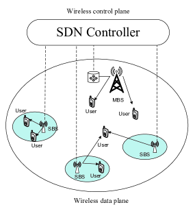
Figure 1: A software defined heterogeneous network with small cell cooperation

II-A Small Cell Offloading

In the HetNet, the deployment of small cell BSs is able to offload users from the MBSs. It can ease the traffic burden of the MBSs and improve the system’s performance to some extent. For example, CRE of the small cells is a common way to offload users from the MBS tier and increases the coverage. In any case, the existing study focuses on the offloading ability of a single small cell. Besides, MBS can reduce its dynamic power consumption when it is lightly loaded. Offloading users to SBSs when they can offer better communication quality can reduce the load of MBS and possibly reduce the energy consumption of the entire network. In our study, we analyze the offloading performance of the cooperation of small cells. For simplicity, the resource partition between different tiers is not considered.

In this scenario, a user is allowed to access any tier’s BSs because of open access. We consider a cell association based on maximum received-signal-strength (RSS). Covered by the closest MSB and SBS, the user will choose one that offers higher RSS as its serving BS [7]. Thus a user is always associated to either an MBS or an SBS.

II-A1 Non-cooperative model

A user will associate with the BS that results in the highest RSS. As the BSs belonging to the same tier have the same transmit power, it means a user will choose its closest MBS or SBS as its serving BS. It’s called the non-cooperative operation. We use association probability to measure the traffic offloading.

Lemma 1.

The probability that a user associates with SBS tier can be expressed as

$$\mathcal{P_{\textnormal{sbs\_no}}}=\frac{1}{1+\frac{\lambda_{m}}{\lambda_{s}}\left(\frac{P_{m}}{P_{s}}\right)^{\frac{2}{\alpha}}}.$$ (1)

Proof:

$P_{m}r_{m}^{-\alpha}$ and $P_{s}r_{s}^{-\alpha}$ are the RSS received by the typical user from its nearest MBS and SBS respectively. The user will access to the tier which can offer it stronger RSS. Therefore

$$\mathcal{\mathcal{P_{\textnormal{sbs\_no}}}} = 1-\mathbb{P}\left(\mathnormal{P_{m}r_{m}^{-\alpha}>P_{s}r_{s}^{-\alpha}}\right)$$

$$= 1-\mathbb{E_{\mathnormal{r_{m}}}\left[\mathbb{P}\left(\mathnormal{r_{s}}>\left(\mathnormal{r_{m}^{\alpha}P_{s}/P_{m}}\right)^{\mathrm{1/\alpha}}\right)\right]}$$

$$= 1-\int_{0}^{\infty}\mathbb{P}\left(\mathnormal{r_{s}}>\left(\mathnormal{r^{\alpha}P_{s}/P_{m}}\right)^{\mathrm{1/\alpha}}\right)\mathnormal{f_{r_{m}}\left(r\right)\textrm{d}r},$$

where $r_{m}$ and $r_{s}$ are the distances from the typical user to its nearest MBS and SBS and its probability density functions (PDFs) are $f_{r_{m}}\left(r\right)$ and $f_{r_{s}}\left(r\right)$. It is known that the null probability of the 2-D homogeneous PPP with density $\lambda$ in an area $A$ is $\exp\left(-\lambda A\right)$, so $\mathnormal{r_{s}}>\left(\mathnormal{r_{m}^{\alpha}P_{s}/P_{m}}\right)^{\mathrm{1/\alpha}}$ means that there’s no BS in the circle whose radius is $\left(\mathnormal{r_{m}^{\alpha}P_{s}/P_{m}}\right)^{\mathrm{1/\alpha}}$ in the small cell tier. Thus,

$$\mathbb{P}\left(\mathnormal{r_{s}}>\left(\mathnormal{r^{\alpha}P_{s}/P_{m}}\right)^{\mathrm{1/\alpha}}\right)=\textrm{e}^{\left(-\lambda_{s}\pi r^{2}\left(P_{s}/P_{m}\right)^{2/\alpha}\right)},$$ (2)

and it is proved in [49] that

$$f_{r_{m}}\left(r\right)=\frac{\textrm{d}\left(1-\mathbb{P}\left[\mathnormal{r_{m}>r}\right]\right)}{\textrm{d}r}=2\pi\lambda_{m}r\textrm{e}^{(-\pi\lambda_{m}r^{2})}.$$ (3)

Then by solving the exponential integral, it can be simplified as (1). ∎

From the above, we can see that in order to change the load of each tier, it just needs to adjust the BS density and power ratio $\lambda_{m}/\lambda_{s}$ and $P_{m}/P_{s}$. Although deploying more SBSs will bring extra costs, the tendency of small cell densification has proved that the capacity of heterogeneous networks can be dramatically improved. Comparing with the method of adjusting transmit powers, deploying more SBSs seems to be a more reasonable way to offload users from MBS.

II-A2 Cooperative model

To meet the exponential growth of traffic demands, small cell densification is a promising way. As small cells are getting closer, cooperation can benefit more. In our proposed network model, the SDN controller coordinates the cooperation among SBSs by gathering information, such as channel states, BSs and users. It decouples processing from transmission within the data plane to make cooperation practically feasible. We call the cooperative small cells an SBS cluster. In the cooperative operation, the cooperative cluster consists of $k$ closest small cells, denoted by $\mathcal{C\subset\mathsf{\Phi_{\mathnormal{s}}}}$. The cooperative small cells jointly transmit a message to the typical user. In other words, the user will associate with the cooperative cluster or the MBS depending on its RSS. The association probability of the cooperative model is

$$\mathcal{P_{\textrm{sbs\_co}}} = \mathbb{P\left(\mathnormal{\overset{{\scriptstyle x_{s,k}}}{\underset{{\scriptstyle x_{s,j}\in\mathcal{C}}}{\sum}}P_{s}r_{s,j}^{-\alpha}>P_{m}r_{m}^{-\alpha}}\right)}$$ (4)

$$= \int\limits_{\stackrel{{\scriptstyle{\scriptstyle 0<r_{s,1}<r_{s,2...}}}}{{r_{s,k-1}<r_{s,k}<\infty}}}\textrm{e}^{\left(-\lambda_{m}\pi\eta^{2/\alpha}\right)}f_{\Gamma}\left(\textbf{r}\right)\textrm{d}\textbf{r{,}}$$

where $\eta=P_{m}/\left(P_{s}\overset{{\scriptstyle x_{s,k}}}{\underset{{\scriptstyle x_{s,j}\in\mathcal{C}}}{\sum}}r_{s,j}^{-\alpha}\right)$ and $r_{s,j}$ denotes the distance of the $j$-th closest small cell to the typical user.

It can be proved by referring to Lemma 1. $\mathbf{r}=[r_{s,1},r_{s,2},....,r_{s,k-1},r_{s,k}]$ is the set of the distances of the $k$ closest small cells to the typical user.

Lemma 2.

The joint PDF of $r_{s,j}$ is

$$f_{\Gamma}\left(\textbf{r}\right)=\left(2\pi\lambda_{s}\right)^{k}\textrm{e}^{\left(-\lambda_{s}\pi r_{s,k}^{2}\right)}\overset{{\scriptstyle x_{s,k}}}{\underset{{\scriptstyle x_{s,j}\in\mathcal{C}}}{\prod}}r_{s,j}.$$ (5)

Proof:

We start from the first and second closest neighbor SBSs. We define $f_{r_{s,2}\mid r_{s,1}}\left(r_{s,2}\mid r_{s,1}\right)$ as the conditional PDF of the distance of the second closest SBS. Around the typical user, with radiuses of $r_{s,1}$ and $r_{s,2}$, it forms an annulus. In analogy to (3), the probability that there’s no SBS in this annulus is $\exp\left(-\lambda_{s}\pi\left(r_{s,2}^{2}-r_{s,1}^{2}\right)\right)$. So,

$$f_{r_{s,2}\mid r_{s,1}}\left(r_{s,2}\mid r_{s,1}\right)=2\pi\lambda_{s}\textrm{e}^{\left(-\lambda_{s}\pi\left(r_{s,2}^{2}-r_{s,1}^{2}\right)\right)}r_{s,2},$$

and by using Bayes formula, we have

$$f_{r_{s,2},r_{s,1}}\left(r_{s,2},r_{s,1}\right) = f_{r_{s,2}\mid r_{s,1}}\left(r_{s,2}\mid r_{s,1}\right)f_{r_{s}}\left(r\right)$$

$$= \left(2\pi\lambda_{s}\right)^{2}\textrm{e}^{\left(-\lambda_{s}\pi r_{s,2}^{2}\right)}r_{s,1}r_{s,2}.$$

In a similar way, we can easily obtain the joint PDF of the $k$-th closest cooperative SBSs expressed as (5). ∎

It’s obvious that the SBS cluster can offer stronger RSS comparing with the single SBS association. So it will offload more users to the small cell tier. But it adds extra complexity to both the transmit side and receive side.

So in the non-cooperative model, we define $\mathcal{\mathrm{\mathnormal{A}}_{\mathrm{m}}}$ ($\mathcal{\mathrm{\mathnormal{A}}_{\mathrm{s}}}$) as the event that the user connects to an MBS (SBS). In the cooperative model, we define $\mathcal{\mathrm{\mathnormal{B}}}_{m}$ ($\mathcal{\mathrm{\mathnormal{B}}}_{s}$) as the event that the user connects to an MBS (SBS cluster).

Small cell cooperation will offload more users from the MBS tier and provide better coverage performance compared with a single small cell. The communication quality will improve dramatically especially for the cell-edge users. In addition, cooperation is also an effective means to reduce interferences. However, cooperation is a complex work for small cells to perform, and deploying more cells causes additional costs in the future.

II-B Power Consumption Model

We consider the power consumption in a Voronoi cell [16] consisting of an MBS and several users. A Voronoi cell associated with a given MBS is the set of all points in $\mathbb{R^{\mathrm{2}}}$ which are closer to it than to any other MBSs. The power consumption is load-dependent for MBSs, and to a lesser extent for SBSs [50]. We introduce SDN controller to manage the power control of BSs. Utilizing the load information of the BS, the SDN controller notifies the BS to turn on/off some channels for dynamically adjusting the BS power consumption.

II-B1 Non-cooperative model

The power consumption of an MBS is proportional to its current load, which is the number of users associated with it. The total power consumption of the MBS under non-cooperative model is

$$P_{\textrm{mbs\_no}}=P_{ms}+nP_{max}\left(\mathcal{\mathrm{1-}P}_{\textnormal{sbs\_no}}\right)/N,$$ (7)

where $P_{ms}$ denotes the static power expenditure, such as processing unit and radio module. $P_{max}$ is the maximum output power. $n$ is the number of users in the Voronoi cell, $N$ is the maximum number of the users when the MBS is full loaded and quality of communication can also be guaranteed in the meantime. $n\left(\mathcal{\mathrm{1-}P}_{\textnormal{sbs\_no}}\right)$ denotes the number of users connecting to the MBS. The output power is determined by the ratio $n\left(\mathcal{\mathrm{1-}P}_{\textnormal{sbs\_no}}\right)/N$.

Since the power consumption of small cell is low and most part of it is static consumption which is $P_{s}$, we assume the energy consumption of the small cells which the users in the Voronoi cell associate with is

$$P_{\textrm{sbs\_no}}=n\mathcal{P}_{\textnormal{sbs\_no}}P_{s}.$$ (8)

We define the total power consumption of the system as the energy needed to serve all the users in the Voronoi cell, which is $P_{\textrm{no}}=P_{\textrm{mbs\_no}}+P_{\textrm{sbs\_no}}$.

II-B2 Cooperative model

In the cooperative model, as more users choose the small cell tier, the number of users connecting to MBS turns to $n\left(\mathrm{1-}P_{\textrm{sbs\_co}}\right)$, so the total energy consumption of the MBS is

$$P_{\textrm{mbs\_co}}=P_{ms}+nP_{max}\mathcal{\left(\mathrm{1-}P_{\textrm{sbs\_co}}\right)}/N.$$ (9)

If $k$ small cells cooperate, that means a user is served by $k$ BSs simultaneously. Due to the low power consumption of small cell, it can be assumed that there are totally $knP_{\textrm{sbs\_co}}$ small cells serving for users in a Voronoi cell. So the energy consumption of the small cells is

$$P_{\textrm{sbs\_co}}=kn\mathcal{P}_{\textrm{sbs\_co}}\left(P_{s}+P_{bkh}\right).$$ (10)

$P_{bkh}$ is the backhaul power consumption for each cooperative SBS. To serve a common user, the cooperative SBSs have to share data with each other, so the backhaul overhead has to be considered. When traffic load of MBS is offloaded to SBS, the dynamic power consumption of MBS decreases. This will be more remarkable in the cooperative model.

So the total power consumption for the cooperative model is $P_{\textrm{co}}=P_{\textrm{mbs\_co}}+P_{\textrm{sbs\_co}}$.

III SINR Coverage and Energy Efficiency

In this section, we analyze the offloading performance through three main metrics: SINR coverage, user rates, and energy efficiency. First, we will discuss the SINR for downlink transmission at a typical user under different association strategies. Then, we derive the analytical expressions for the coverage probability and the average ergodic rate. On the basis of the above analysis, we can get the energy efficiency of the system under both cooperative and non-cooperative schemes.

III-A SINR Coverage Probability

The received signal at a typical user can be written as

$$\underset{\mathit{{\scriptstyle x_{i,j}\in\mathcal{B}}}}{\sum}\frac{\left(Ph_{i,j}\right)^{1/2}}{r_{i,j}^{\alpha/2}}X+\underset{x_{i,j}\notin\mathit{\mathbb{\mathcal{B}}}}{\sum}\frac{\left(Ph_{i,j}\right)^{1/2}}{r_{i,j}^{\alpha/2}}Y+Z,$$ (11)

where $P$ is the transmit power of the serving BS. $\mathcal{B}$ denotes the set of BSs that the user associate with, it may be an MBS, an SBS or an SBS cluster. $X$ denotes the input symbol that is sent by the associated BSs. So the first sum denotes the useful signal from the associated BSs. $Y$ denotes the input symbol sent by the BSs that do not belong to $\mathcal{B}$. So the second sum denotes the interference, including the inter-tier and intra-tier interference. $Z$ is a circular-symmetric zero-mean complex Gaussian random variable with variance $\sigma^{2}$, which models the additive white noise.

Thus, from [21] and [51], the received instantaneous SINR at a typical user is given by

$$\mathrm{SINR\left(\mathcal{B}\right)=\frac{\mid\underset{\mathit{{\scriptstyle x_{i,j}\in\mathcal{B}}}}{\sum}\mathnormal{\left(Ph_{i,j}\right)^{1/2}r_{i,j}^{-\alpha/\mathrm{2}}}\mid^{2}}{\mathnormal{\mid\underset{\mathit{{\scriptstyle x_{i,j}\notin\mathcal{B}}}}{\sum}\left(Ph_{i,j}\right)^{1/2}r_{i,j}^{-\alpha/2}\mid^{2}+\sigma^{2}}}}.$$ (12)

The coverage probability is defined as the probability that the received SINR is greater than a threshold. For a given SINR threshold $\theta$, the coverage probability $\mathcal{P}_{n}$ at the typical user can be expressed as

$$\mathcal{P}_{n}=\mathbb{P\left(\mathrm{SINR>\theta}\right)},$$ (13)

and $\mathcal{P}_{n}$ is relevant to the user’s association policy.

Lemma 3.

To connect the link between the coverage and the association policy, we analyze the PDFs of the distance between a typical user and its serving BS or BSs, i.e., $f_{R}\left(r\right)$. In the non-cooperative model, when the user connects to an MBS or an SBS, the PDFs are respectively

$$f_{Rm}\left(r\right)=\frac{2\pi\lambda_{m}r}{1-\mathcal{P_{\textnormal{sbs\_no}}}}\textrm{e}^{\left(-\pi r^{2}\left(\lambda_{m}+\lambda_{s}\left(P_{s}/P_{m}\right)^{2/\alpha}\right)\right)},$$ (14)

and

$$f_{Rs}\left(r\right)=\frac{2\pi\lambda_{s}r}{\mathcal{P_{\textnormal{sbs\_no}}}}\textrm{{{e}}}^{\left(-\pi r^{2}\left(\lambda_{s}+\lambda_{m}\left(P_{m}/P_{s}\right)^{2/\alpha}\right)\right)}.$$ (15)

As the association probability changes, the distance distribution changes as well. In the cooperative model, the PDF of the distance between the user and the MBS is

$$f_{Rcm}\left(r\right)=\frac{f_{r_{m}}\left(r\right)g(r)}{1-P_{\textnormal{sbs\_co}}},$$ (16)

where $\mathbb{\mathnormal{g(r)=}P}\left(\mathnormal{\mathnormal{P_{m}r^{-\alpha}/P_{s}>\mathnormal{\overset{{\scriptstyle x_{s,k}}}{\underset{{\scriptstyle x_{s,j}\in\mathcal{C}}}{\sum}}r_{s,j}^{-\alpha}}}}\right)$ is the function of $r$. $f_{r_{m}}\left(r\right)$ is given as (3).

If the user connects to an SBS cluster, the joint PDF is

$$f_{Rcs}\left(\textbf{r}\right) = \frac{1}{P_{\textnormal{sbs\_co}}}\textrm{e}^{\left(-\pi\lambda_{m}\eta^{2/\alpha}\right)}f_{\Gamma}\left(\textbf{r}\right).$$ (17)

Proof:

See Appendix A. ∎

Remark 4.

Note that there is no general analytical expression for $g(r)$ in (16), we can derive an exact result for a special case for simplicity, as shown later in our simulation. Here, we consider two SBSs cooperation and $\alpha=4$. So we have

$$g(r)=\int_{0}^{\frac{\pi}{4}}\frac{\pi\lambda_{s}\sin^{-1}\varphi+\omega r^{-2}}{\left(\cos\varphi r^{-1}\right)^{2}\omega}\textrm{e}^{\left(-\frac{\pi\lambda_{s}r^{2}}{\omega\sin\varphi}\right)}\textrm{d}\varphi,$$ (18)

where $\omega=\sqrt{P_{m}/P_{s}}$.

Proof:

See Appendix B. ∎

Theorem 5.

The coverage probabilities for a typical user associated with an MBS, an SBS in non-cooperative model are

$$\mathcal{P}_{n}\left(A_{m}\right)=\int_{r>0}\left[\textrm{e}^{\left(-P_{m}^{-1}\theta r^{\alpha}\sigma^{2}\right)}\mathcal{L_{\mathnormal{I}}\left(\mathnormal{P_{m}^{-1}}\mathnormal{\theta r^{\alpha}}\right)}\right]f_{Rm}\left(r\right)\textrm{d}r,$$ (19)

$$\mathcal{P}_{n}\left(A_{s}\right)=\int_{r>0}\left[\textrm{e}^{\left(-P_{s}^{-1}\theta r^{\alpha}\sigma^{2}\right)}\mathcal{L_{\mathnormal{I}}\left(\mathnormal{\mathnormal{P_{s}^{-1}}\theta r^{\alpha}}\right)}\right]f_{Rs}\left(r\right)\textrm{d}r,$$ (20)

where distance distributions are given in Lemma 3. And

$$\mathcal{L}_{\mathnormal{I}}\left(\mathnormal{s}\right)=\overset{}{\underset{i\in\left\{s,m\right\}}{\prod}}\textrm{e}^{\left(-2\pi\lambda_{i}\left(sP_{i}\right)^{2/\alpha}\mathcal{F\left(\mathnormal{\left(sP_{i}\right)^{\mathnormal{-1/\alpha}}d_{i},\alpha}\right)}\right)}.$$ (21)

It denotes the Laplace transform of interference $I$. $d_{i}$ is the minimum distance between the user and its nearest interfering BS in tier $i$, $i\in\left\{s,m\right\}.$ It means all interfering BSs are distributed outside the circle with the radius $d_{i}$. For (19), we have $d_{m}=r$ and $d_{s}=\omega^{-2/\alpha}r$. For (20), we have $d_{m}=\omega^{2/\alpha}r$ and $d_{s}=r$. And

$$\mathcal{F\left(\mathnormal{y,\alpha}\right)=\intop}_{y}^{\infty}\frac{\mu}{1+\mu^{\alpha}}\textrm{d}\mu.$$ (22)

Proof:

See Appendix C. ∎

Since the association methods are mutually exclusive, by using the law of total probability, we obtain the overall coverage probability of the non-cooperative model as follow:

$$\mathcal{P}_{\textrm{no}}=\left(1-\mathcal{P}_{\mathnormal{\textrm{sbs\_no}}}\right)\mathcal{P}_{n}\left(A_{m}\right)+\mathcal{P}_{\mathnormal{\textrm{sbs\_no}}}P_{n}\left(A_{s}\right),$$ (23)

where $\mathcal{P}_{\mathnormal{\textrm{sbs\_no}}}$ is given in (1).

In view of the big advantage in transmit power, MBS can offer better coverage performance than the SBS under the same threshold $\theta$. In addition, an SBS user may be subjected to more cross-tier interference.

Remark 6.

We can get the closed-form expressions for specific values of the integral function (22) [21]. Then we can get $\mathcal{F}\mathnormal{\left(y,4\right)}=\frac{1}{2}\tan^{-1}\left(y^{-2}\right).$ Note that in the interference-limited network, when $\sigma^{2}$ is small enough, the first exponential term in (19) and (20) approaches $1$. Here, in consideration of the situation and conciseness of the numerical analysis, assuming $\alpha=4$ and $\sigma^{2}=0$, we have the result $\mathcal{P}_{n}\left(A_{m}\right)=\mathcal{P}_{n}\left(A_{s}\right)$. And the total outage probability (23) simplifies to

$$\mathcal{P}_{\textrm{no}}=\frac{1}{1+\sqrt{\theta}\tan^{-1}\left(\sqrt{\theta}\right).}$$ (24)

For this special case, the total outage probability in the non-cooperative model is just the function of threshold $\theta$ and there exists a negative correlation between them. This is the same as the result in [52], where the coverage probability has nothing to do with the number of the tiers or their densities and transmit powers in an interference-limited network. The adjustment in the properties of the BSs is helpless to improve the coverage performance. In other words, we can deploy more BSs to improve the throughput and ignoring the interference they cause.

Theorem 7.

In the cooperative model, when the user associates with an MBS we can obtain its coverage probability $\mathcal{P}_{n}\left(B_{m}\right)$ by substituting $f_{Rcm}\left(r\right)$ for $f_{Rm}\left(r\right)$ in (19). When the user associates with an SBS cluster, its coverage probability $\mathcal{P}_{\mathnormal{n}}\left(B_{s}\right)$ is shown as (25). Same as the coverage probabilities in non-cooperative model, for $\mathcal{P}_{n}\left(B_{m}\right)$ we have $d_{m}=r$ and $d_{s}\thickapprox\omega^{-2/\alpha}r$. And for $\mathcal{P}_{n}\left(B_{s}\right)$, we have $d_{m}=\eta^{1/\alpha}$ and $d_{s}=r_{s,k}$.

Proof:

See Appendix C. ∎

$$\mathcal{P}_{n}\left(B_{s}\right)=\int\limits_{\stackrel{{\scriptstyle{\scriptstyle 0<r_{s,1}<r_{s,2...}}}}{{r_{s,k-1}<r_{s,k}<\infty}}}\left[\exp\left(\frac{-\theta\sigma^{2}}{\overset{{\scriptstyle x_{s,k}}}{\underset{{\scriptstyle x_{s,j}\in\mathcal{C}}}{\sum}}P_{s}r_{s,j}^{-\alpha}}\right)\mathcal{L_{\mathnormal{I}}\left(\frac{\mathnormal{\theta}}{\mathnormal{\overset{{\scriptstyle x_{s,k}}}{\underset{{\scriptstyle x_{s,j}\in\mathcal{C}}}{\sum}}P_{s}r_{s,j}^{-\alpha}}}\right)}\right]f_{Rcs}\left(\textbf{r}\right)\textrm{d}\textbf{r}$$ (25)

 

The overall coverage probability of the user in the cooperative model is

$$\mathcal{P}_{\textrm{co}}=\left(1-\mathcal{P}_{\mathnormal{\textrm{sbs\_co}}}\right)\mathcal{P}_{n}\left(B_{m}\right)+\mathcal{P}_{\mathnormal{\textrm{sbs\_co}}}\mathcal{P}_{n}\left(B_{s}\right).$$ (26)

When $k=1$, (25) degrades into (20). In the SBS tier, if the user associates with only one BS, its second nearest neighbor BS becomes its strongest interference. Same for the $k$-th nearest neighbor. So if we bring in cooperation, the strongest interference turns into useful signal. As $k$ increases, this advantage will be more obvious. Even two SBSs cooperate, it may have a better coverage performance than the MBS user. For the cell-edge users who are far from the MBS, a single SBS is not able to satisfy its requirements for communication. Cooperation could solve this problem. Because cooperation needs BSs to exchange data with each other, simply increasing $k$ is not an optimal solution. And it is also not practical for the mobile users to connect to too many BSs at the same time.

III-B Mean Achievable Rate

With the conditional coverage probability above, we can easily obtain the mean achievable rates (measured in (bit/sec/Hz)) of non-cooperative and cooperative models respectively.

Theorem 8.

The achievable rate of a typical user can be expressed as

$$\tau=\frac{1}{\ln 2}\int_{0}^{\infty}\mathcal{P}_{n}\frac{1}{1+\theta}\mathbb{\mathnormal{\textrm{d}\theta}},$$ (27)

where $\mathcal{P}_{n}$ is the coverage probability of the given user. After substituting $\mathcal{P}_{n}\left(A_{m}\right),\mathcal{P}_{n}\left(A_{s}\right),\mathcal{P}_{n}\left(B_{m}\right)$ and $\mathcal{P}_{n}\left(B_{s}\right)$ into (27), we can get the achievable rates when user associates to the corresponding BS, which are $\tau_{\textrm{mbs}}$, $\tau_{\textrm{sbs}}$ and $\tau_{\textrm{mbs\_co}}$, $\tau_{\textrm{mbs\_co}}$.

Proof:

The mean achievable rate of the typical user is defined as

$$\tau = \mathbb{E}\left[\mathnormal{\log\mathnormal{{}_{2}}\left(\mathnormal{\textrm{1}}+\mathrm{SINR}\right)}\right]$$

$$= \frac{1}{\ln 2}\mathbb{E\left[\mathnormal{\ln\left(\mathnormal{\textrm{1}}+\mathrm{SINR}\right)}\right]}$$

$$= \frac{1}{\ln 2}\int_{0}^{\infty}\mathbb{P}\left(\mathrm{SINR}>\textrm{e}^{t}-1\right)\textrm{d}t$$

$$= \frac{1}{\ln 2}\int_{0}^{\infty}\mathbb{P}\left(\mathrm{SINR}>\theta\right)\frac{1}{1+\theta}\textrm{d}\theta.$$

Here using the change of variables and the definition of the coverage probability (13) we can obtain the final result. ∎

According to the mutual independence of different association strategy, by using the law of total probability, we get the mean achievable rate for a user in non-cooperative model as

$$\tau_{\textrm{no}}=\left(1-\mathcal{P}_{\mathnormal{\textrm{sbs\_no}}}\right)\tau_{\mathnormal{\textrm{mbs}}}+\mathcal{P}_{\mathnormal{\textrm{sbs\_no}}}\tau_{\mathnormal{\textrm{sbs}}}.$$ (28)

Similarly, the mean achievable rate in the cooperative model is

$$\tau_{\textrm{co}}=\left(1-\mathcal{P}_{\mathnormal{\textrm{sbs\_co}}}\right)\tau_{\mathnormal{\textrm{mbs\_co}}}+\mathcal{P}_{\mathnormal{\textrm{sbs\_co}}}\tau_{\mathnormal{\textrm{sbs\_co}}}.$$ (29)

III-C Energy Efficiency

Energy efficiency is one of the key performance indicators for the proposed model. We define it as the ratio of throughput to the energy consumption of the network (usually measured in (bits/J)). It is assumed that BSs in different tiers share the same frequency bandwidth $B$. Since we have derived the achievable rate $\tau$, the throughput of a typical user is $\tau B$. For a Voronoi cell, it includes all the BSs that serve the users in the cell. Numbers of the users and BSs are given in II-B. The total system throughput of the non-cooperative model and cooperative model are respectively derived as

$$R_{\textrm{no}}=n\tau_{\textrm{no}}B,$$ (30)

and

$$R_{\textrm{co}}=n\tau_{\textrm{co}}B.$$ (31)

Thus, the expressions of the corresponding energy efficiency of the non-cooperative model and cooperative model are

$$\mathcal{E}_{\mathrm{\textrm{no}}}=R_{\textrm{no}}/P_{\textrm{no}},$$ (32)

and

$$\mathcal{E}_{\textrm{$\mathrm{\textrm{co}}$}}=R_{\textrm{co}}/P_{\textrm{co}}$$ (33)

respectively.

IV Numerical Results

In this section, the traffic offloading performance with cooperative and non-cooperative models has been compared by numerical results. Without loss of generality, two small cells cooperative scenarios are analyzed and $\sigma^{2}=0$ is configured in numerical simulations. The comparison is performed in terms of coverage probability, association probability, average achievable rate and energy efficiency.

IV-A Coverage Probability

Fig. 2 shows the coverage probability trends with SINR threshold corresponding to event $A_{m}$, $A_{s}$, $B_{m}$ and $B_{s}$. The coverage probability decreases as the SINR threshold increases. The curves of the SBS and MBS are the same in non-cooperative model. In this interference-limited regime, the user just connects to a BS that offers the highest RSS without differentiating between the tiers. When two SBSs cooperates the coverage probability has been dramatically improved and is higher than the coverage probability transmitted by an MBS.

Fig. 3 depicts the overall coverage probabilities of the non-cooperative and cooperative model with respect to the SINR threshold. The overall coverage probability with the non-cooperative and cooperative model decreases with the increase of the SINR threshold. When the SINR threshold has been fixed, the overall coverage probability with the cooperative model is higher than that of the non-cooperative model. It demonstrates that the cooperation can offer better coverage.

Fig. 4 shows the effect of SBS density and the transmit power of MBS on the overall coverage probability in the cooperative model. As the SBS density grows, coverage probabilities increase and this trend slows down gradually when $\lambda_{s}/\lambda_{m}$ is larger than 30. That’s because the user will associate with the SBS cluster with a significant possibility if $\lambda_{s}$ is big enough. As the transmit power of MBS $P_{m}$ increases, there’s more chance that the user will associate with an MBS. But based on the result in Fig. 3, the SBS cooperation offer a better coverage. So the overall coverage probability decreases with the increase of $P_{m}$.

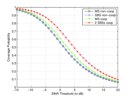
Figure 2: Coverage probabilities when the user connects to different BSs. $\alpha=4,$ $\lambda_{m}=\left(500^{2}\pi\right)^{-1}$, $\lambda_{s}=50\lambda_{m}$ and $P_{m}=50$, $P_{s}=1$.

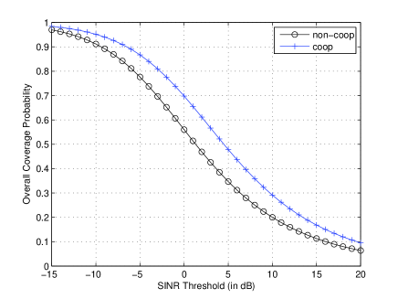
Figure 3: Overall coverage probability of the non-cooperative and cooperative model where $\lambda_{m}=\left(500^{2}\pi\right)^{-1}$, $\lambda_{s}=50\lambda_{m}$ and $P_{m}=50$, $P_{s}=1$.

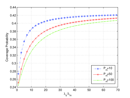
Figure 4: Overall coverage probability of the cooperative model under different $P_{m}$ and $\lambda_{s}$. $\lambda_{m}=\left(500^{2}\pi\right)^{-1}$ $\theta=5$ and $P_{s}=1$.

IV-B Traffic load

As mentioned in II-A, we use association probability to evaluate small cell offloading. It can be seen from Fig. 5, if small cells are deployed denser, they will have more chance to serve the user. And the rising trends recede as $\lambda_{m}$ increases. The association probability of cooperative model always outperforms the non-cooperative model owe to the large RSS of the SBS cooperation.

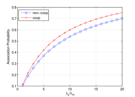
Figure 5: Comparison of the association probability between non-cooperative and cooperative model where $\alpha=3$, $\lambda_{m}=\left(500^{2}\pi\right)^{-1}$ and $P_{m}=50$, $P_{s}=2$.

IV-C Energy Efficiency

Fig. 6 gives the mean achievable rate of a typical user in the two models. We still focus on the impact of the small cell density. According to the figure, the user rate is constant as $\lambda_{s}$ increases. We can see from (27) that user rate is deduced from the coverage probability. (24) is independent with the cell densities and transmit power, so there’s no doubt that the mean achievable rate is invariant for $\lambda_{s}/\lambda_{m}$ in the non-cooperative model. In the cooperative model, the rate is a rising curve and the trend is steady. Deploying more SBSs brings the SBSs closer to the user, thus SINR and rate of the user becomes higher.

Fig. 7 shows the energy efficiency of the non-cooperative and cooperative model in a Voronoi cell. The shape of the curves is as similar with that of the user rate shown in Fig. 6. In the non-cooperative model, the energy efficiency decreases with the increase of the $\lambda_{s}/\lambda_{m}$. This really distracts from our main goal. In the cooperative model, when $\lambda_{s}<3\lambda_{m}$ the energy efficiency experiences a slight decrease. When $\lambda_{s}>3\lambda_{m}$ it keeps up increase. Considering the result in Fig. 5 , when $\lambda_{s}$ is small, user is more likely to associate with the MBS other than the cooperative SBSs. When $\lambda_{s}=6\lambda_{m}$, the two curves meet and $\mathcal{E}_{\mathrm{\textrm{co}}}$ starts to transcend $\mathcal{E}_{\textrm{$\mathrm{no}$}}$. Hence, we can draw the conclusion that small cell offloading through cooperation have better energy efficiency in a dense environment.

In our work, we analyze $n$ users in a Voronoi cell where there’s one MBS and several SBSs to serve these users. The number of SBSs is decided by $n$ and is constant, and many of the SBSs may even locate outside the Voronoi cell. In the cooperative model, as $\lambda_{s}$ increases, there won’t be more SBSs to serve these $n$ users, thus the energy consumption won’t increase significantly. Meanwhile, an increase in $\lambda_{s}$ means the SBSs are closer to the users, so the user rate will improve through cooperation. These changes make EE improves as $\lambda_{s}$ increases.

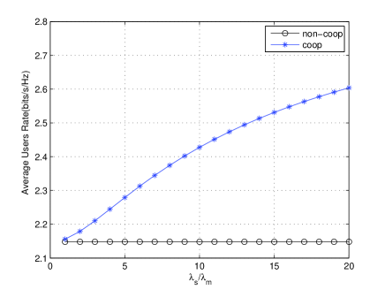
Figure 6: Mean achievable rate of the non-cooperative and cooperative model where $\alpha=4$, $\lambda_{m}=\left(500^{2}\pi\right)^{-1}$, $P_{m}=50$, $P_{s}=2$ and $B=20\textrm{MHz}$.

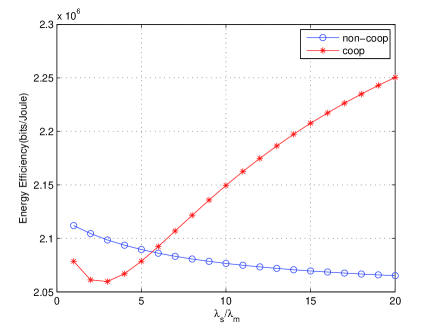
Figure 7: The system’s energy efficiency of the non-cooperative and cooperative model where $\alpha=4$, $\lambda_{m}=\left(500^{2}\pi\right)^{-1}$, $P_{m}=50$, $P_{s}=2$, $B=20\textrm{MHz}$ and $P_{ms}=20,$ $P_{bkh}=1$.

V Conclusions

In this paper, we have proposed a novel offloading strategy through small cell cooperation. Using tools from stochastic geometry, a tractable model has been proposed in the downlink HetNets. The SDN controller has been introduced to manage the SBS cooperation and power control, which simplifies the BS’s function and burden. In proposed cooperative-model, two or more small cells could serve a common user simultaneously. The user connects to an MBS or an SBS cluster depending on its RSS. In our study the power consumption of BS is determined by its load, which is represented by the association probability. We obtain the expressions of the overall coverage probabilities, achievable rate for a typical user with and without cooperation. Numerical results have shown that small cell cooperation could offload more users from MBS tier. It can also increase the system’s coverage performance. It’s been proved that when SBSs get closer, cooperation can benefit more and thus shows the great potential of small cell densification.

Appendix A Proof of Lemma 3

$f_{R}\left(r\right)$ is a conditional PDF under different association circumstance. So for the MBS association in non-cooperative model, the probability of the event of $\mathnormal{R_{m}}\mathnormal{>r}$ is

$$\mathbb{P}\left[\mathnormal{R_{m}}\mathnormal{>r}\right] = \mathbb{P}\left[\mathnormal{r_{m}}\mathnormal{>r}\mid A_{m}\right]$$ (34)

$$= \frac{\mathbb{P}\left[\mathnormal{r_{m}}\mathnormal{>r},A_{m}\right]}{\mathbb{P}\left[\mathnormal{A_{m}}\right]}$$

$$= \frac{\mathbb{P}\left[\mathnormal{r_{m}}\mathnormal{>r},\mathnormal{\mathnormal{P_{m}r_{m}^{-\alpha}>P_{s}r_{s}^{-\alpha}}}\right]}{1-\mathcal{P_{\textnormal{sbs\_no}}}}$$

$$= \frac{\int_{r}^{\infty}\mathbb{P}\left[\mathnormal{\mathnormal{r_{s}>r\omega^{\mathnormal{-2/\alpha}}}}\right]f_{r_{m}}\left(r\right)\textrm{d}r}{1-\mathcal{P_{\textnormal{sbs\_no}}}},$$

where $\mathnormal{r_{m}}$ is the distance of the nearest MBS, $\mathbb{P}\left[\mathnormal{\mathnormal{r_{s}>\left(P_{s}r^{\alpha}/P_{m}\right)^{\mathnormal{1/\alpha}}}}\right],$ $f_{r_{m}}\left(r\right)$ and $\mathcal{P_{\textnormal{sbs\_no}}}$ can be found in Lemma 1. Then we can get $f_{Rm}\left(r\right)=\frac{\textrm{d}\mathbb{P\left[\mathnormal{r_{m}}\mathnormal{>r}\mid\mathnormal{A_{m}}\right]}}{\textrm{d}r}.$ Proofs of (15) is the same under the condition of $A_{s}$.

For (16),

$$\mathbb{P}\left[\mathnormal{r_{m}}\mathnormal{>r},\mathnormal{B_{m}}\right] = \mathbb{P}\left[\mathnormal{r_{m}}\mathnormal{>r},\mathnormal{\mathnormal{P_{m}r_{m}^{-\alpha}>\mathnormal{\overset{{\scriptstyle x_{s,k}}}{\underset{{\scriptstyle x_{s,j}\in\mathcal{C}}}{\sum}}P_{s}r_{s,j}^{-\alpha}}}}\right]$$ (35)

$$= \int_{r}^{\infty}\left(\mathbb{P}\left(\mathnormal{\mathnormal{r<\eta^{\mathnormal{1/\alpha}}}}\right)\right)f_{r_{m}}\left(r\right)\textrm{d}r.$$

For (17), we can get joint probability

$$\mathbb{P}\left[\mathnormal{r_{m}}\mathnormal{>r},\mathnormal{B_{s}}\right]=\int\limits_{\stackrel{{\scriptstyle{\scriptstyle 0<r_{s,1}<r_{s,2...}}}}{{r_{s,k-1}<r_{s,k}<\infty}}}\mathbb{P}\left[\mathnormal{r>\eta}^{1/\alpha}\right]f_{\Gamma}\left(\textbf{r}\right)\textrm{d{r}}$$ (36)

as similar with the numerator in (34). After the multiple integral we can obtain the result.

Appendix B Proof of Remark 4

The proof of (18) is under the condition that $k=2$ and $\alpha=4$. So

$$g\left(r\right) = \mathbb{P\mathnormal{\left(\omega^{\mathnormal{2}}r^{\mathnormal{-4}}>\mathnormal{r_{s,1}^{\mathnormal{-4}}}+\mathnormal{r_{s,2}^{\mathnormal{-4}}}\right)}}$$ (37)

$$= \mathbb{P}\mathnormal{\left(\left(\omega r^{\mathnormal{-2}}\right)^{\mathnormal{2}}>\left(\mathnormal{r_{\mathnormal{s,1}}^{\mathnormal{-2}}}\right)^{\mathnormal{2}}+\left(\mathnormal{\mathnormal{r_{s,2}^{-2}}}\right)^{\mathnormal{2}}\right)},$$

so this probability is constrained in an area which within a circle with radius $\omega r^{-2}$ and the area $0<r_{s,1}<r_{s,2}<\infty.$ Set $a=\mathnormal{\mathnormal{r_{\mathnormal{s,1}}^{\mathnormal{-2}}}}$ and $b=\mathnormal{\mathnormal{r_{s,2}^{-2}}}$, the joint probability of $a$ and $b$ can be expressed as

$$f_{a,b}\left(a,b\right)=\left|\begin{array}[]{c}\textrm{J}\end{array}\right|f_{r_{s,2},r_{s,1}}\left(a^{-\frac{1}{2}},b^{-\frac{1}{2}}\right),$$ (38)

where Jacob determinant $\mid\textrm{J}\mid=\left|\begin{array}[]{cc}\frac{\textrm{d}r_{s,1}}{\textrm{d}a}&0\\ 0&\frac{\textrm{d}r_{s,2}}{\textrm{d}b}\end{array}\right|=\frac{1}{4}\left(ab\right)^{-\frac{3}{2}}$.

As it concerned to the circle area, we use the polar transformation, so $a=\rho\cos\varphi$ and $b=\rho\sin\varphi$. Finally we have

$$g\left(r\right)=\int_{0}^{\frac{\pi}{4}}\textrm{d}\varphi\int_{0}^{\omega r^{-2}}\rho f_{a,b}\left(\rho\cos\varphi,\rho\sin\varphi\right)\textrm{d}\rho,$$ (39)

after solving the inner integration, we can obtain (18).

Appendix C Proof of Theorem 5 and Theorem 7

The proof of (19), (20) and (25) are similar. We take (19) as an example. For the user served by an MBS, SINR can be expressed as

$$\mathrm{SINR=\frac{\mathnormal{P_{m}h_{m,1}r_{m}^{-\alpha}}}{\mathnormal{I+\mathnormal{\sigma^{2}}}}},$$ (40)

where $I=I_{M}+I_{s}$ and $I_{M}=\underset{i\in m}{\sum}\mathnormal{P_{m}h_{m,i}^{\mathnormal{2}}r_{m,i}^{-\alpha}}$, $I_{s}=\underset{i\in s}{\sum}\mathnormal{P_{s}h_{s,i}^{\mathnormal{2}}r_{s,i}^{-\alpha}}$ are the interference from the MBS tier and SBS tier.

So the coverage probability when user associated with an MBS in non-cooperative model is

$$\mathcal{P}_{n}\left(A_{m}\right)$$

$$= \mathbb{P}\left(\mathrm{SINR>\theta}\right)$$

$$= \mathbb{\int_{\mathnormal{r>0}}P\left[\mathrm{SINR}>\theta\mid\mathnormal{r}\right]\mathnormal{f_{Rm}\left(r\right)dr}}$$

$$\underset{=}{{\scriptstyle\left(a\right)}} \int_{\mathnormal{r>0}}\mathbb{P}\left[h_{m,1}>P_{m}^{-1}\theta r_{m}^{\alpha}\left(I+\sigma^{2}\right)\mid\mathnormal{r}\right]f_{Rm}\left(r\right)\textrm{d}r$$

$$= \mathbb{\int_{\mathnormal{r>0}}E}_{I}\left[\textrm{e}^{\left(-P_{m}^{-1}\theta r_{m}^{\alpha}\left(I+\sigma^{2}\right)\right)}\right]f_{Rm}\left(r\right)\textrm{d}r$$

$$= \int_{\mathnormal{r>0}}\mathbb{E}\left[\textrm{e}^{\left(-P_{m}^{-1}\theta r_{m}^{\alpha}\sigma^{2}\right)}\mathcal{L}_{I}\left(P_{m}^{-1}\theta r_{m}^{\alpha}\right)\right]f_{Rm}\left(r\right)\textrm{d}r,$$

where $f_{Rm}\left(r\right)$ can be seen in Lemma 3. $\left(a\right)$ is because that $h_{i,j}\sim exp(1)$. $\mathcal{L}_{I}\left(s\right)$ is Laplace transform of interference $I$, it can be written as

$$\mathcal{L}_{I}\left(s\right) = \mathbb{E}_{I}\left[\textrm{e}^{-sI}\right]$$

$$= \overset{}{\underset{i\in\left\{s,m\right\}}{\prod}}\mathbb{E}\left[\underset{\Phi_{I_{i}}}{\prod}\textrm{e}^{-sP_{i}h_{i,j}r_{i,j}^{-\alpha}}\right]$$

$$= \overset{}{\underset{i\in\left\{s,m\right\}}{\prod}}\mathbb{E}\left[\underset{\Phi_{I_{i}}}{\prod}\mathbb{E}_{h_{i,j}}\left(\textrm{e}^{-sP_{i}h_{i,j}r_{i,j}^{-\alpha}}\right)\right]$$

$$\overset{{\scriptstyle\left(b\right)}}{=} \overset{}{\underset{i\in\left\{s,m\right\}}{\prod}}\mathbb{E}\left[\underset{\Phi_{I_{i}}}{\prod}\frac{1}{1+sP_{i}r_{i,j}^{-\alpha}}\right]$$

$$\overset{{\scriptstyle\left(c\right)}}{=} \overset{}{\underset{i\in\left\{s,m\right\}}{\prod}}\textrm{e}^{\left(-\lambda_{i}\int_{\mathbb{R}^{2}}\left(1-\frac{1}{1+sP_{i}r^{-\alpha}}\right)\textrm{d}r\right)}$$

$$\overset{{\scriptstyle\left(d\right)}}{=} \overset{}{\underset{i\in\left\{s,m\right\}}{\prod}}\textrm{e}^{\left(-2\pi\lambda_{i}\int_{d}^{\infty}\left(1-\frac{1}{1+sP_{i}r{}^{-\alpha}}\right)r\textrm{d}r\right)}$$

$$\overset{{\scriptstyle\left(e\right)}}{=} \overset{}{\underset{i\in\left\{s,m\right\}}{\prod}}\textrm{e}^{\left(-2\pi\lambda_{i}\left(sP_{i}\right)^{\frac{2}{\alpha}}\right)\int_{\left(sP_{i}\right)^{-\frac{1}{\alpha}}d}^{\infty}\frac{\mu}{1+\mu^{\alpha}}\textrm{d}\mu},$$

where $(b)$ uses the expression for moment generating function of an exponential random variable, which is $h_{i,j}$; $(c)$ is due to the probability generating functional for a PPP; $\left(d\right)$ uses the translation of surface integration. $\left(e\right)$ is because of the variable substitution $\mu^{\alpha}=\left(sP_{i}\right)^{-1}r^{\alpha}.$ $\Phi_{I_{i}}$ is the set of all the interference BSs in tier $i$. And the interference is expressed as the integration from $d$ to $\infty.$ When $i\in m$, that is in MBS tier, interference is outside the coverage area of the user’s serving MBS which is the circle of radius $r$. So we set $d=r$. As our discussion is limited in the event of $A_{m}$, we have the condition $\mathnormal{\mathnormal{r_{s}>\left(P_{s}r^{\alpha}/P_{m}\right)^{\mathnormal{1/\alpha}}}}$. In which, $r_{s}$ also means the distance of nearest interference SBS. So $i\in s$, $d=r_{s}=\left(P_{s}r^{\alpha}/P_{m}\right)^{1/\alpha}.$ Similarly for $\mathcal{P}_{n}\left(B_{m}\right)$, when $i\in s$, $\mathnormal{\overset{{\scriptstyle x_{s,k}}}{\underset{{\scriptstyle x_{s,j}\in\mathcal{C}}}{\sum}}r_{s,j}^{-\alpha}>P_{m}r_{m}^{-\alpha}/P_{s}}$, to obtain the region of $r_{s,1}$ we have to get the approximation $r_{s,1}^{-\alpha}>P_{m}r_{m}^{-\alpha}/P_{s}$. So $d\thickapprox\left(\frac{P_{s}}{P_{m}}\right)^{1/\alpha}$.

Tao Han (M’13) received the Ph.D. degree in information and communication engineering from Huazhong University of Science and Technology (HUST), Wuhan, China, in 2001. He is currently an Associate Professor with the School of Electronic Information and Communications, HUST. From 2010 to 2011, he was a Visiting Scholar with the University of Florida, Gainesville, FL, USA, as a Courtesy Associate Professor. He has published more than 50 papers in international conferences and journals. His research interests include wireless communications, multimedia communications, and computer networks. He is currently serving as an Area Editor for the European Alliance Innovation Endorsed Transactions on Cognitive Communications.

Yujie Han received the Bachelor’s degree in communication and information system from Huazhong University of Science and Technology, Wuhan, China, in 2012, where he is currently working toward the Master’s degree. His research interests include cooperative communication, stochastic geometry, and heterogeneous networks.

Xiaohu Ge (M’09-SM’11) is currently a full Professor with the School of Electronic Information and Communications at Huazhong University of Science and Technology (HUST), China. He is an adjunct professor with the Faculty of Engineering and Information Technology at University of Technology Sydney (UTS), Australia. He received his PhD degree in Communication and Information Engineering from HUST in 2003. He has worked at HUST since Nov. 2005. Prior to that, he worked as a researcher at Ajou University (Korea) and Politecnico Di Torino (Italy) from Jan. 2004 to Oct. 2005. His research interests are in the area of mobile communications, traffic modeling in wireless networks, green communications, and interference modeling in wireless communications. He has published more than 100 papers in refereed journals and conference proceedings and has been granted about 15 patents in China. He received the Best Paper Awards from IEEE Globecom 2010. Dr. Ge is a Senior Member of the China Institute of Communications and a member of the National Natural Science Foundation of China and the Chinese Ministry of Science and Technology Peer Review College. He has been actively involved in organizing more the ten international conferences since 2005. He served as the general Chair for the 2015 IEEE International Conference on Green Computing and Communications (IEEE GreenCom 2015). He serves as an Associate Editor for the IEEE ACCESS, Wireless Communications and Mobile Computing Journal (Wiley) and the International Journal of Communication Systems (Wiley), etc. Moreover, he served as the guest editor for IEEE Communications Magazine Special Issue on 5G Wireless Communication Systems.

Qiang Li (M’16) received the B.Eng. degree in communication engineering from the University of Electronic Science and Technology of China (UESTC), Chengdu, China, in 2007 and the Ph.D. degree in electrical and electronic engineering from Nanyang Technological University (NTU), Singapore, in 2011. From 2011 to 2013, he was a Research Fellow with Nanyang Technological University. Since 2013, he has been an Associate Professor with Huazhong University of Science and Technology, Wuhan, China. He was a visiting scholar at the University of Sheffield, Sheffield, UK from March to June 2015. His current research interests include future broadband wireless networks, software-defined networking, cooperative communications, and cognitive spectrum sharing.

Jing Zhang (M’13) received the M.S. and Ph.D. degrees in electronics and information engineering from Huazhong University of Science and Technology (HUST), Wuhan, China, in 2002 and 2010, respectively. He is currently an Associate Professor with HUST. He has done research in the areas of multiple-input multiple-output, CoMP, beamforming, and next-generation mobile communications. His current research interests include cellular systems, green communications, channel estimation, and system performance analysis.

Zhiquan Bai (M’08) received the M.Eng. degree in communication and information systems from Shandong University, Jinan, China, in 2003, and the Ph.D. degree in communication engineering with honor from INHA University in 2007, under the Grant of Korean Government IT Scholarship, Incheon, Korea. From 2007 to 2008, he was a postdoctor with UWB Wireless Communications Research Center, INHA University, Incheon, Korea. Since 2007, he has been an associate professor with the School of Information Science and Engineering, Shandong University, China. He has published more than 70 papers in international conferences and journals. His current research interests include cooperative communications and MIMO system, ultra wideband communications, cognitive radio system, and beyond-fourth generation wireless communications. Dr. Bai is the associate editor of the Introduction Journal of Communication Systems. He served as a TPC member and a session chair for some international conferences.

Lijun Wang (M’16) received the B.S. degree in telecommunication engineering from Xidian University, Xi’an, China in July, 2004 and the M.S. degree in communication and information system from Huazhong University of Science and Technology (HUST), Wuhan, China in June, 2008. From Sept., 2016 she will work toward the Ph.D. degree with Wuhan University, Wuhan, China. She is currently an associate professor with the Department of Information Science and Technology, Wenhua College, Wuhan, China. Her research interests include wireless communications, and multimedia communications.

References

- [1] Y. Zhang, M. Chen, S. Mao, L. Hu, and V. Leung, “Cap: community activity prediction based on big data analysis,” IEEE Network, vol. 28, no. 28, pp. 52–57, 2014.
- [2] P. Popovski, V. Braun, G. Mange, P. Fertl, D. Gozalvez-Serrano, N. Bayer, H. Droste, A. Roos, G. Zimmermann, M. Fallgren et al., “Ic t-317669-metis/d6. 2 initial report on horizontal topics, first results and 5g system concept,” EU-Project METIS (ICT-317669), 2014.
- [3] X. Ge, H. Cheng, M. Guizani, and T. Han, “5g wireless backhaul networks: challenges and research advances,” IEEE Network, vol. 28, no. 6, pp. 6–11, 2014.
- [4] M. Chen, Y. Zhang, Y. Li, M. Hassan, and A. Alamri, “Aiwac: Affective interaction through wearable computing and cloud technology,” IEEE Wireless Communications, vol. 22, no. 1, pp. 20–27, 2015.
- [5] M. Chen, Y. Zhang, Y. Li, and S. Mao, “Emc: Emotion-aware mobile cloud computing in 5g,” IEEE Network, vol. 29, no. 2, pp. 32–38, 2015.
- [6] A. Damnjanovic, J. Montojo, Y. Wei, T. Ji, T. Luo, M. Vajapeyam, T. Yoo, O. Song, and D. Malladi, “A survey on 3gpp heterogeneous networks,” IEEE Wireless Communications, vol. 18, no. 3, pp. 10–21, 2011.
- [7] H. ElSawy, E. Hossain, and D. I. Kim, “Hetnets with cognitive small cells: user offloading and distributed channel access techniques,” IEEE Communications Magazine, vol. 51, no. 6, pp. 28–36, 2013.
- [8] J. G. Andrews, H. Claussen, M. Dohler, S. Rangan, and M. C. Reed, “Femtocells: Past, present, and future,” IEEE Journal on Selected Areas in Communications, vol. 30, no. 3, pp. 497–508, 2012.
- [9] R. Razavi and H. Claussen, “Urban small cell deployments: Impact on the network energy consumption,” in Wireless Communications and Networking Conference Workshops (WCNCW). IEEE, 2012, pp. 47–52.
- [10] T. Han, Y. Yang, X. Ge, and G. Mao, “Mobile converged networks: framework, optimization, and challenges,” IEEE Wireless Communications, vol. 21, no. 6, pp. 34–40, 2014.
- [11] M. Chen, Y. Zhang, L. Hu, T. Taleb, and Z. Sheng, “Cloud-based wireless network: Virtualized, reconfigurable, smart wireless network to enable 5g technologies,” Mobile Networks and Applications, vol. 20, no. 6, pp. 1–9, 2015.
- [12] D. Gesbert, S. Hanly, H. Huang, S. S. Shitz, O. Simeone, and W. Yu, “Multi-cell mimo cooperative networks: A new look at interference,” IEEE Journal on Selected Areas in Communications, vol. 28, no. 9, pp. 1380–1408, 2010.
- [13] O. Simeone, O. Somekh, H. V. Poor, and S. Shamai, “Local base station cooperation via finite-capacity links for the uplink of linear cellular networks,” IEEE Transactions on Information Theory, vol. 55, no. 1, pp. 190–204, 2009.
- [14] R. Irmer, H. Droste, P. Marsch, M. Grieger, G. Fettweis, S. Brueck, H.-P. Mayer, L. Thiele, and V. Jungnickel, “Coordinated multipoint: Concepts, performance, and field trial results,” IEEE Communications Magazine, vol. 49, no. 2, pp. 102–111, 2011.
- [15] V. Garcia, Y. Zhou, and J. Shi, “Coordinated multipoint transmission in dense cellular networks with user-centric adaptive clustering,” IEEE Transactions on Wireless Communications, vol. 13, no. 8, pp. 4297–4308, 2014.
- [16] F. Baccelli and A. Giovanidis, “A stochastic geometry framework for analyzing pairwise-cooperative cellular networks,” IEEE Transactions on Wireless Communications, vol. 14, no. 2, pp. 794–808, 2015.
- [17] B. Nunes, M. Mendonca, X.-N. Nguyen, K. Obraczka, T. Turletti et al., “A survey of software-defined networking: Past, present, and future of programmable networks,” IEEE Communications Surveys Tutorials, vol. 16, no. 3, pp. 1617–1634, 2014.
- [18] D. Kreutz, F. M. Ramos, P. Esteves Verissimo, C. Esteve Rothenberg, S. Azodolmolky, and S. Uhlig, “Software-defined networking: A comprehensive survey,” Proceedings of the IEEE, vol. 103, no. 1, pp. 14–76, 2015.
- [19] M. Arslan, K. Sundaresan, and S. Rangarajan, “Software-defined networking in cellular radio access networks: potential and challenges,” IEEE Communications Magazine, vol. 53, no. 1, pp. 150–156, 2015.
- [20] L. E. Li, Z. M. Mao, and J. Rexford, “Toward software-defined cellular networks,” in European Workshop on Software Defined Networking (EWSDN). IEEE, 2012, pp. 7–12.
- [21] G. Nigam, P. Minero, and M. Haenggi, “Coordinated multipoint joint transmission in heterogeneous networks,” IEEE Transactions on Communications, vol. 62, no. 11, pp. 4134–4146, 2014.
- [22] H.-S. Jo, Y. J. Sang, P. Xia, and J. G. Andrews, “Heterogeneous cellular networks with flexible cell association: A comprehensive downlink sinr analysis,” IEEE Transactions on Wireless Communications, vol. 11, no. 10, pp. 3484–3495, 2012.
- [23] X. Ge, B. Yang, J. Ye, and G. Mao, “Spatial spectrum and energy efficiency of random cellular networks,” IEEE Transactions on Communications, vol. 63, no. 3, pp. 1019–1030, 2015.
- [24] R. Tanbourgi, S. Singh, J. G. Andrews, and F. K. Jondral, “A tractable model for noncoherent joint-transmission base station cooperation,” IEEE Transactions on Wireless Communications, vol. 13, no. 9, pp. 4959–4973, 2014.
- [25] ——, “Analysis of non-coherent joint-transmission cooperation in heterogeneous cellular networks,” in IEEE International Conference on Communications (ICC). IEEE, 2014, pp. 5160–5165.
- [26] D. Lee, H. Seo, B. Clerckx, E. Hardouin, D. Mazzarese, S. Nagata, and K. Sayana, “Coordinated multipoint transmission and reception in lte-advanced: deployment scenarios and operational challenges,” IEEE Communications Magazine, vol. 50, no. 2, pp. 148–155, 2012.
- [27] X. Ge, S. Tu, T. Han, and Q. Li, “Energy efficiency of small cell backhaul networks based on gauss-markov mobile models,” IET Networks, vol. 4, no. 2, pp. 158–167, 2015.
- [28] X. Ge, J. Ye, Y. Yang, and Q. Li, “User mobility evaluation for 5g small cell networks based on individual mobility model,” IEEE Journal on Selected Areas in Communications, vol. 34, no. 3, pp. 528–541, 2016.
- [29] X. Mi, Z. Tian, X. Xu, M. Zhao, and J. Wang, “No stack: A sdn-based framework for future cellular networks,” in International Symposium on Wireless Personal Multimedia Communications (WPMC). IEEE, 2014, pp. 497–502.
- [30] D. Cao, S. Zhou, and Z. Niu, “Optimal combination of base station densities for energy-efficient two-tier heterogeneous cellular networks,” IEEE Transactions on Wireless Communications, vol. 12, no. 9, pp. 4350–4362, 2013.
- [31] T. Q. Quek, W. C. Cheung, and M. Kountouris, “Energy efficiency analysis of two-tier heterogeneous networks,” in Wireless Conference 2011-Sustainable Wireless Technologies (European Wireless). VDE, 2011, pp. 1–5.
- [32] X. Ge, S. Tu, G. Mao, and C. X. Wang, “5g ultra-dense cellular networks,” IEEE Wireless Communications, vol. 23, no. 1, pp. 72–79, 2016.
- [33] P. Qiao, Y. Zhong, and W. Zhang, “Base station cooperation for energy efficiency: A gauss-poisson process approach,” in Signal and Information Processing Association Annual Summit and Conference (APSIPA). IEEE, 2013, pp. 1–7.
- [34] W. Nie, X. Wang, F.-C. Zheng, and W. Zhang, “Energy-efficient base station cooperation in downlink heterogeneous cellular networks,” in IEEE Globecom. IEEE, 2014, pp. 1779–1784.
- [35] L. Saker, S. E. Elayoubi, T. Chahed, and A. Gati, “Energy efficiency and capacity of heterogeneous network deployment in lte-advanced,” in European 18th European Wireless Conference Wireless (EW 2012). VDE, 2012, pp. 1–7.
- [36] Y. Sun, Y. Chang, S. Song, and D. Yang, “An energy-efficiency aware sleeping strategy for dense multi-tier hetnets,” in IEEE Globecom Workshops. IEEE, 2014, pp. 1180–1185.
- [37] D. Lopez-Perez, X. Chu, and . Guvenc, “On the expanded region of picocells in heterogeneous networks,” IEEE Journal of Selected Topics in Signal Processing, vol. 6, no. 3, pp. 281–294, 2012.
- [38] A. K. Gupta, H. S. Dhillon, S. Vishwanath, and J. G. Andrews, “Downlink multi-antenna heterogeneous cellular network with load balancing,” IEEE Transactions on Communications, vol. 62, no. 11, pp. 4052–4067, 2014.
- [39] S. Singh and J. G. Andrews, “Joint resource partitioning and offloading in heterogeneous cellular networks,” IEEE Transactions on Wireless Communications, vol. 13, no. 2, pp. 888–901, 2014.
- [40] Q. Liu, G. Feng, and S. Qin, “Energy-efficient traffic offloading in macro-pico networks,” in Wireless and Optical Communication Conference (WOCC). IEEE, 2013, pp. 236–241.
- [41] K. Son, S. Chong, and G. Veciana, “Dynamic association for load balancing and interference avoidance in multi-cell networks,” IEEE Transactions on Wireless Communications, vol. 8, no. 7, pp. 3566–3576, 2009.
- [42] Q. Ye, B. Rong, Y. Chen, M. Al-Shalash, C. Caramanis, and J. G. Andrews, “User association for load balancing in heterogeneous cellular networks,” IEEE Transactions on Wireless Communications, vol. 12, no. 6, pp. 2706–2716, 2013.
- [43] H. Kim, G. De Veciana, X. Yang, and M. Venkatachalam, “Alpha-optimal user association and cell load balancing in wireless networks,” in Proc. IEEE INFOCOM. IEEE, 2010, pp. 1–5.
- [44] L. Liu, X. Chen, M. Bennis, G. Xue, and Z. Han, “A distributed admm approach for mobile data offloading in software defined network,” in IEEE Wireless Communications and Networking Conference (WCNC). IEEE, 2015, pp. 1748–1752.
- [45] Z. Arslan, M. Erel, Y. Ozcevik, and B. Canberk, “Sdoff: A software-defined offloading controller for heterogeneous networks,” in IEEE Wireless Communications and Networking Conference (WCNC). IEEE, 2014, pp. 2827–2832.
- [46] Y. Li and M. Chen, “Software-defined network function virtualization: A survey,” IEEE Access, vol. 3, pp. 2542–2553, 2015.
- [47] M. Chen, Y. Qian, S. Mao, W. Tang, and X. Yang, “Software-defined mobile networks security,” Mobile Networks and Applications, pp. 1–15, 2015.
- [48] Y. Li, F. Zheng, M. Chen, and D. Jin, “A unified control and optimization framework for dynamical service chaining in software-defined nfv system,” IEEE Wireless Communications, vol. 22, no. 6, pp. 15–23, 2015.
- [49] V. Baumstark and G. Last, “Some distributional results for poisson-voronoi tessellations,” Advances in applied probability, pp. 16–40, 2007.
- [50] G. Auer, V. Giannini, C. Desset, I. Godor, P. Skillermark, M. Olsson, M. A. Imran, D. Sabella, M. J. Gonzalez, O. Blume et al., “How much energy is needed to run a wireless network?” IEEE Wireless Communications, vol. 18, no. 5, pp. 40–49, 2011.
- [51] A. H. Sakr and E. Hossain, “Location-aware cross-tier coordinated multipoint transmission in two-tier cellular networks,” IEEE Transactions on Wireless Communications, vol. 13, no. 11, pp. 6311–6325, 2014.
- [52] H. S. Dhillon, R. K. Ganti, F. Baccelli, and J. G. Andrews, “Modeling and analysis of k-tier downlink heterogeneous cellular networks,” IEEE Journal on Selected Areas in Communications, vol. 30, no. 3, pp. 550–560, 2012.