Statistics of the epoch of reionization (EoR) 21-cm signal – II. The evolution of the power spectrum error-covariance

Abstract

The EoR 21-cm signal is expected to become highly non-Gaussian as reionization progresses. This severely affects the error-covariance of the EoR 21-cm power spectrum which is important for predicting the prospects of a detection with ongoing and future experiments. Most earlier works have assumed that the EoR 21-cm signal is a Gaussian random field where (1) the error-variance depends only on the power spectrum and the number of Fourier modes in the particular $k$ bin, and (2) the errors in the different $k$ bins are uncorrelated. Here we use an ensemble of simulated 21-cm maps to analyze the error-covariance at various stages of reionization. We find that even at the very early stages of reionization ($\bar{x}_{\rm\text{H\,{i}}}\sim 0.9$) the error-variance significantly exceeds the Gaussian predictions at small length-scales ($k>0.5\,{\rm Mpc}^{-1}$) while they are consistent at larger scales. The errors in most $k$ bins (both large and small scales), are however found to be correlated. Considering the later stages ($\bar{x}_{\rm\text{H\,{i}}}=0.15$), the error-variance shows an excess in all $k$ bins within $k\geq 0.1\,{\rm Mpc}^{-1}$, and it is around $200$ times larger than the Gaussian prediction at $k\sim 1\,{\rm Mpc}^{-1}$. The errors in the different $k$ bins are all also highly correlated, barring the two smallest $k$ bins which are anti-correlated with the other bins. Our results imply that the predictions for different 21-cm experiments based on the Gaussian assumption underestimate the errors, and it is necessary to incorporate the non-Gaussianity for more realistic predictions.

1 Introduction

The Epoch of Reionization (EoR) is an important period in the history of our universe. During this era the hydrogen in our universe gradually changed its state from being neutral (H i) to ionized (H ii). Our knowledge in this regard is guided so far by two major observational constraints. The measurements of the Thomson scattering optical depth of the cosmic microwave background (CMB) photons from the free electrons (e.g. Komatsu et al. 2011; Planck Collaboration et al. 2015, 2016a, 2016b etc.) and the observations of the Lyman-$\alpha$ absorption spectra of the high redshift quasars (e.g. Becker et al. 2001; Fan et al. 2003; White et al. 2003; Goto et al. 2011; Becker et al. 2015 etc.). These observations together suggest that this epoch probably extended over a wide redshift range $6\lesssim z\lesssim 12$ (e.g. Mitra et al. 2011, 2013, 2015; Robertson et al. 2013; Robertson et al. 2015; Planck Collaboration et al. 2016a etc.). However, most of the fundamental issues associated with this epoch, such as the properties of sources contributing to the ionization photon budget, gradual evolution in their properties, topology of the brightness temperature maps at different stages of the reionization etc. remain unknown till date.

The brightness temperature fluctuations of the 21-cm signal originating due to the hyperfine transition in the neutral hydrogen has the potential to probe this rather complex epoch. There is considerable effort underway to detect the EoR 21-cm signal through radio interferometry using e.g. the GMRT (Paciga et al., 2013), LOFAR (Yatawatta et al., 2013; van Haarlem et al., 2013), MWA (Tingay et al., 2013; Bowman et al., 2013; Dillon et al., 2014) and PAPER (Parsons et al., 2014; Jacobs et al., 2015; Ali et al., 2015). Apart from these first generation radio interferometers, the detection of this signal is also one of the key science goals of the future radio telescopes such as the SKA (Mellema et al., 2013; Koopmans et al., 2015) and HERA (Furlanetto et al., 2009).

In the recent past a significant amount of effort has gone into in making quantitative predictions of the sensitivity of different ongoing and upcoming experiments to measure the 21-cm signal through its power spectrum (e.g. Morales 2005; McQuinn et al. 2006; Beardsley et al. 2013 etc.). The majority of these studies have been done by simulating the expected EoR 21-cm signal and incorporating the specific telescope response to it (e.g. Thomas et al. 2009; Jensen et al. 2013; Pober et al. 2014; Majumdar et al. 2016 etc.).

The redshifted 21-cm signal is largely dominated by different foregrounds which are $\sim 4-5$ orders of magnitude stronger than the signal (Ali et al., 2008; Bernardi et al., 2009; Ghosh et al., 2012; Pober et al., 2013; Moore et al., 2015). Modelling these foregrounds accurately and removing them from the actual data is the major obstacle in detecting the cosmological 21-cm signal. In this work, we assume that the foregrounds can be removed accurately, and we only focus entirely on the signal.

Power spectrum estimation for the EoR 21-cm signal is restricted by statistical uncertainties inherent to the measurements. A part of these uncertainties arises due to the system noise which is Gaussian, and depends on the instrument and the total observation time. It may happen that in some observations the system noise dominates the total error budget. However the system noise can, in principle, be made arbitrarily small by increasing the observation time and we do not consider the system noise in the present work. Apart from the system noise, any statistical cosmological signal always comes with an intrinsic uncertainty which is known as the cosmic variance. While taking into account the effect of this cosmic variance in their measurements, all of the above mentioned sensitivity estimation studies have effectively assumed that the system noise and the EoR 21-cm signal are both independent Gaussian random variables. This is possibly a valid assumption as long as reionization is at its early stages and one is looking at sufficiently large scale power of the signal. During the early stages of the EoR, the H i is expected to trace the underlying matter distribution. As reionization proceeds, creation and growth of the ionized regions introduces non-Gaussianity (Bharadwaj & Pandey, 2005; Mondal et al., 2015) in the H i field. The simple assumption of the signal to be a Gaussian random variable for power spectrum error estimates does not hold. It is necessary to quantify the uncertainties correctly to obtain a proper interpretation of the signal.

Mondal et al. (2015) have first studied how the non-Gaussianities present in the H i distribution during the EoR affect the error predictions for the 21-cm power spectrum. If the signal were a Gaussian random field, one would expect the signal-to-noise ratio (SNR) to scale as the square-root of the number of independent measurements. Using a large ensemble of statistically independent realizations of EoR 21-cm signal, they have shown that for a fixed observational volume, it is not possible to achieve a SNR above a certain limiting value $[{\rm SNR}]_{l}$, even if one increases the number of independent Fourier modes that goes into the estimation of the power spectrum of the signal. They have also demonstrated that the non-Gaussianity present in the EoR 21-cm signal, which is mainly driven by the distribution of the H ii regions, gradually increases with the increasing volume and number of these H ii regions as reionization progresses. At a fixed redshift $z=8$, they have considered different values of global neutral fraction $\bar{x}_{\rm\text{H\,{i}}}$ and shown that the value of $[{\rm SNR}]_{l}$ falls with the progress in reionization. The non-Gaussian effects play an important role in the error predictions for the EoR 21-cm power spectrum particularly in the later stages of the EoR.

Building up on the work of Mondal et al. (2015), in Mondal et al. (2016) (hereafter Paper I) we presented a detailed and generic theoretical frame work to interpret and quantify the effect of non-Gaussianity on the error estimates for the 21-cm power spectrum through the error-covariance $\textbf{{C}}_{ij}$. Using the analytic calculation, we have identified two sources of contribution to the $\textbf{{C}}_{ij}$. One is the usual variance for a Gaussian random field and the other is the non-Gaussian component which is quantified through the trispectrum. We validated this theoretical frame work using a large ensemble of simulated EoR 21-cm signal at a fixed neutral fraction of $\sim 0.5$, for two different simulation volumes. This analysis established the fact that, due to the non-Gaussianity, not only the different Fourier modes $\tilde{T}_{\rm b}(k)$ but also the errors in the power spectrum estimated in different $k$ bins, are correlated. There are significant correlations between the errors at the small length scales and between the small and the large length scale. We also observed a small anti-correlation between the errors in the smallest and the intermediate $k$ values. It is important to note that the theoretical frame work established and used in Mondal et al. (2015) and Paper I are very generic and not limited only to the EoR 21-cm signal but can be applied to the analysis of any non-Gaussian cosmological signal such as the galaxy redshift surveys (Hamilton et al., 2006; Neyrinck & Szapudi, 2008; Neyrinck, 2011; Harnois-Déraps & Pen, 2013; Mohammed & Seljak, 2014; Carron et al., 2015).

The entire analysis of Paper I was done at a fixed redshift ($=8$) and neutral fraction ($\approx 0.5$). It does not address the issue of how the error-covariance evolves with the evolving non-Gaussianity in the signal as reionization progresses. In this paper, as a follow up of Paper I, we study the evolution of the error-covariance of the 21-cm power spectrum more generally with the evolving redshift and neutral fraction as ionization of the IGM progresses during the EoR. Here we identify the different sources that contribute to the non-Gaussianity and subsequently to the $\textbf{{C}}_{ij}$. We test the theoretical formalism for interpreting the error-covariance of the power spectrum presented in Paper I for these evolving simulated H i fields. We further identify the length scale ranges where the non-Gaussianity becomes significant (or in other words the trispectrum contribution to the error-covariance is significant) and how those evolve. We also try to investigate the causes of correlation and anti-correlation between the errors in the power spectrum estimated in different $k$ bins.

The structure of this paper is as follows. In section 2, we briefly summarize the theoretical formalism presented in Paper I for interpreting the error-covariance of the power spectrum. We describe our semi-numerical simulations which are used to generate the ensembles of the EoR 21-cm signal in section 3. In section 4, we describe our results i.e. the estimated power spectrum error-covariance at different stages of reionization. Finally, in section 5, we discuss and summarize our findings.

Throughout this paper, we have used the Planck+WP best fit values of cosmological parameters $\Omega_{\rm m0}=0.3183$, $\Omega_{\rm\Lambda 0}=0.6817$, $\Omega_{\rm b0}h^{2}=0.022032$, $h=0.6704$, $\sigma_{8}=0.8347$, and $n_{\rm s}=0.9619$ (Planck Collaboration et al., 2014).

2 The power spectrum error-covariance

In this section we briefly summarize the theoretical formalism for interpreting the EoR 21-cm power spectrum error-covariance $\textbf{{C}}_{ij}$. The reader is refered to Sections 2 and 3 of Paper I for a detailed discussion. We consider $\tilde{T}_{\rm b}(\textbf{{k}})$ which is the Fourier transform of the EoR 21-cm brightness temperature fluctuation $\delta{T_{\rm b}}(\textbf{{x}})={T_{\rm b}}(\textbf{{x}})-\bar{T}_{\rm b}$ in a cubic comoving volume $V$ with periodic boundary conditions. The primary quantity of interest here is the power spectrum $P(k)$ of the brightness temperature fluctuations which is defined as

$$P(\textbf{{k}})=V^{-1}\langle\tilde{T}_{\rm b}(\textbf{{k}})\,\tilde{T}_{\rm b}(-\textbf{{k}})\rangle\,.$$ (1)

We also introduce the trispectrum $T(\textbf{{k}}_{a},\textbf{{k}}_{b},\textbf{{k}}_{c},\textbf{{k}}_{d})$ which is defined through

$$\langle\tilde{T}_{\rm b}(a)\tilde{T}_{\rm b}(b)\tilde{T}_{\rm b}(c)\tilde{T}_{\rm b}(d)\rangle=V^{2}[\,\delta_{a+b,0}~{}\delta_{c+d,0}~{}P(a)P(c)$$

$$+\delta_{a+c,0}~{}\delta_{b+d,0}~{}P(a)P(b)+\delta_{a+d,0}~{}\delta_{b+c,0}~{}P(a)P(b)]$$

$$+V\delta_{a+b+c+d,0}~{}T(a,b,c,d)$$ (2)

where we have used the notation $\tilde{T}_{\rm b}(a)\equiv\tilde{T}_{\rm b}({\textbf{{k}}_{a}})$. Note that the trispectrum is zero for a Gaussian random field.

Here we have considered the bin averaged power spectrum $\bar{P}({k_{i}})$ evaluated in different bins in $k$ space. The bins here are spherical shells of width $\Delta k_{i}$ in Fourier space. We use the binned power spectrum estimator, which for the $i~{}$th bin is defined as

$$\hat{P}(k_{i})=\frac{1}{N_{k_{i}}V}\sum_{\textbf{{k}}}\tilde{T}_{\rm b}(\textbf{{k}})\,\tilde{T}_{\rm b}(-\textbf{{k}})\,,$$ (3)

where $\sum_{\textbf{{k}}}$, $N_{k_{i}}$ and $k_{i}$ respectively refer to the sum, the number and the average comoving wavenumber of all the Fourier modes in the $i~{}$th bin. The ensemble average over many statistically independent realizations of $\tilde{T}_{\rm b}(\textbf{{k}})$ gives the mean bin-averaged power spectrum $\bar{P}({k_{i}})=\langle\hat{P}({k_{i}})\rangle$.

The question of interest here is – ‘How accurately can the power spectrum be estimated from a given EoR 21-cm data set?’. Any estimation of the EoR 21-cm power spectrum is constrained by the errors, and here we only consider the statistical uncertainty which is inherent to the EoR 21-cm signal, the cosmic variance. We quantify this uncertainty through the error-covariance of the binned power spectrum estimator

$$\textbf{{C}}_{ij}=\langle[\hat{P}({k_{i}})-\bar{P}({k_{i}})][\hat{P}({k_{j}})-\bar{P}({k_{j}})]\rangle\,.$$ (4)

The error-covariance $\textbf{{C}}_{ij}$ is found (Paper I) to scale with the volume as $V^{-1}$, and the values of $\textbf{{C}}_{ij}$ are also found to span a very large dynamical range across the $k$ values which we have considered here. It is more convenient to consider the dimensionless form of the error-covariance matrix (equation 33 of Paper I) which is defined as

$$\textbf{{c}}_{ij}=\frac{\textbf{{C}}_{ij}\,V\ k_{i}^{3/2}k_{j}^{3/2}}{(2\pi)^{2}\bar{P}(k_{i})\,\bar{P}(k_{j})}\,.$$ (5)

This does not have any explicit volume dependence, and it has been calculated (equation 34 of Paper I) to be

$$\textbf{{c}}_{ij}=A_{i}^{2}\left(\frac{k_{i}}{\Delta k_{i}}\right)\delta_{ij}+t_{ij}\,.$$ (6)

where the Kronecker delta $\delta_{ij}$ is $1$ if $i=j$ and $0$ otherwise. Here

$$A_{i}=\sqrt{\frac{\overline{P^{2}}(k_{i})}{[\bar{P}(k_{i})]^{2}}}\,.$$ (7)

where

$$\overline{P^{2}}(k_{i})=\frac{1}{N_{k_{i}}}\sum_{\textbf{{k}}}P^{2}(\textbf{{k}})$$ (8)

is the square of the power spectrum averaged over the $i$ th bin. The dimensionless quantity $A_{i}$ is a number of order unity introduced in Mondal et al. (2015). The value of $A_{i}$ is expected to vary from bin to bin. However, these variations are expected to be small, and we may expect a value $A_{i}\approx 1$ in most situations.

The dimensionless bin-averaged trispectrum (equation 35 of Paper I) is defined as

$$t_{ij}=\frac{\bar{T}(k_{i},k_{j})\ k_{i}^{3/2}\,k_{j}^{3/2}}{(2\pi)^{2}\bar{P}(k_{i})\,\bar{P}(k_{j})}\,,$$ (9)

where

$$\bar{T}(k_{i},k_{j})=\frac{1}{N_{k_{i}}N_{k_{j}}}\sum_{\textbf{{k}}_{a}\in i,\textbf{{k}}_{b}\in j}T(\textbf{{k}}_{a},-\textbf{{k}}_{a},\textbf{{k}}_{b},-\textbf{{k}}_{b})$$ (10)

is the average trispectrum, $\textbf{{k}}_{a}$ and $\textbf{{k}}_{b}$ here are summed over the $i~{}$th and the $j~{}$th bins respectively. The trispectrum is zero for a Gaussian random field.

The diagonal elements of the error-covariance $\textbf{{c}}_{ii}$ (equation 6) quantify the variance of the error in the estimated power spectrum. We have $\textbf{{c}}_{ii}=A_{i}^{2}({k_{i}}/{\Delta k_{i}})$ if the EoR 21-cm signal is a Gaussian random field. In our analysis we have used logarithmic binning which implies that $(k_{i}/\Delta k_{i})\approx 1.9$ is nearly constant across all the bins. In this case, we expect $\textbf{{c}}_{ii}$ to have a nearly constant value $\approx 2$ in all the $k$ bins. The EoR 21-cm signal becomes increasingly non-Gaussian as the IGM becomes more and more ionized. This manifests itself as a non-zero contribution from the trispectrum to $\textbf{{c}}_{ii}$. As a consequence the value of $\textbf{{c}}_{ii}$ exceeds the value $\approx 2$ expected for a Gaussian random field. We interpret this excess as arising from the trispectrum which develops when the EoR 21-cm signal becomes non-Gaussian.

The off-diagonal terms of $\textbf{{c}}_{ij}$ quantify the correlations between the errors in the power spectrum estimated at different bins. These terms are all zero i.e. the errors in the different bins are uncorrelated if the EoR 21-cm signal is a Gaussian random field. However, the EoR 21-cm signal becomes increasingly non-Gaussian as reionization progresses, and we expect the off-diagonal terms to develop non-zero values. We interpret any statistically significant non-zero off-diagonal component of $\textbf{{c}}_{ij}$ as arising from the trispectrum which develops when the EoR 21-cm signal becomes non-Gaussian.

We have used equation (6) to interpret the results in the subsequent analysis of this paper. We expect the diagonal elements $\textbf{{c}}_{ii}$ to have a nearly constant value $\approx 2$ and the off-diagonal elements of $\textbf{{c}}_{ij}$ to be zero if the EoR 21-cm signal is a Gaussian random field. We have interpreted any deviations from these values as arising from the trispectrum $t_{ij}$ which arises due to the non-Gaussian nature of the EoR 21-cm signal.

3 Simulating the EoR redshifted 21-cm signal

3.1 The Signal Ensemble (SE)

We have generated the redshifted EoR 21-cm signal using semi-numerical simulations which involve three main steps. First, we use a particle mesh $N$-body code to generate the dark matter distribution at the different redshifts listed in Table 1. We have run simulations with comoving volume $V=[215\,{\rm Mpc}]^{3}$ using $3072^{3}$ grids of spacing $0.07\,{\rm Mpc}$ and a mass resolution of $1.09\times 10^{8}M_{\sun}$. In the next step we use the Friends-of-Friends (FoF) algorithm (Davis et al., 1985) to identify collapsed halos in the dark matter distribution. We have used a fixed linking length of $0.2$ times the mean inter-particle distance and also set the criterion that a halo should have at least $10$ dark matter particles which implies a minimum halo mass of $M_{\rm min}=1.09\times 10^{9}M_{\sun}$.

Table 1: This tabulates the redshifts ($z$) and corresponding mass-averaged neutral fraction ($\bar{x}_{\rm\text{H\,{i}}}$) where we have simulation outputs for the 21-cm signal.

$z$	$\bar{x}_{\rm\text{H\,{i}}}$
13	0.98
11	0.93
10	0.86
9	0.73
8	0.50
7	0.15

The third and final step generates the ionization map based on the excursion set formalism of Furlanetto et al. (2004). It is assumed that the hydrogen traces the dark matter and the halos host the sources which emit the ionizing radiation. It is also assumed that the number of ionizing photons emitted by a source is proportional to the mass of its host halo with the constant of proportionality being quantified through a dimensionless parameter $N_{\rm ion}$. In addition to $N_{\rm ion}$, the simulations have another free parameter $R_{\rm mfp}$ the mean free path of the ionizing photons. We determine whether a grid point is ionized or not by smoothing the hydrogen density field and the photon density field using spheres of different radii starting from $R_{\rm min}$ (the grid size) to $R_{\rm mfp}$. A particular grid point is considered to be ionized if for any smoothing radius the photon density exceeds the hydrogen density at that grid point. The simulated H i distribution is then mapped to the redshift space using the peculiar velocities of the simulation particles to generate 21-cm brightness temperature maps. Our semi-numerical simulations closely follow Choudhury et al. (2009) and Majumdar et al. (2014) to generate the ionization field, and the resulting field is mapped on to redshift space following the methodology of Majumdar et al. (2013). The final ionization maps and the 21-cm brightness temperature maps are generated on a grid that is eight times coarser than the one used for the $N$-body simulations.

\psfrag{xh1}[c][c][1][0]{\Large$\bar{x}_{\rm\text{H\,{i}}}$}\psfrag{z}[c][c][1][0]{\Large$z$}\psfrag{10}[c][c][1][0]{\Large$10$}\includegraphics[width=203.80193pt]{figs/z_xh1.eps}

Figure 1: This shows the reionization history ($\bar{x}_{\rm\text{H\,{i}}}$ as a function of $z$) that we have obtained from our simulations.

It is possible to achieve different reionization histories $\bar{x}_{\rm\text{H\,{i}}}(z)$ by varying the parameters $N_{\rm ion}$ and $R_{\rm mfp}$, $\bar{x}_{\rm\text{H\,{i}}}(z)$ here refers to the mass-averaged H i fractions. The redshift evolution of $\bar{x}_{\rm\text{H\,{i}}}(z)$ during EoR is largely unknown, apart from the fact that the H i reionization ended before a redshift of $6$ (e.g. Becker et al. 2001; Fan et al. 2003; Becker et al. 2015) and the total integrated Thomson scattering optical depth has a value $\tau=0.058\pm 0.012$ (Planck Collaboration et al., 2016a). We have set $R_{\rm mfp}=20\,{\rm Mpc}$ which is consistent with the findings of Songaila & Cowie (2010) from the study of Lyman limit systems at low redshifts. The value of $N_{\rm ion}$ was fixed (at $23.21$) so as to achieve $50\%$ ionization at $z=8$, and the resulting reionization history is shown in Figure 1. We see that reionization is complete by $z\sim 6$ in the resulting reionization history, further we have $\tau=0.057$ which is consistent with the measured optical depth. The values of $\bar{x}_{\rm\text{H\,{i}}}$ obtained from our simulation are tabulated as a function of $z$ in Table 1.

We have run $50$ independent realizations of the simulations to generate an ensemble of $50$ statistically independent realizations of the EoR 21-cm signal We refer to this ensemble as the Signal Ensemble (SE). In summary, the Signal Ensemble (SE) contains $50$ statistically independent realizations of the 21-cm signal for each of the redshifts $z$ and mass-averaged neutral fractions $\bar{x}_{\rm\text{H\,{i}}}$ listed in Table 1. Figure 2 shows two dimensional sections through one realization of the signal for all the $\bar{x}_{\rm\text{H\,{i}}}$ values listed in Table 1. We have used the SE to estimate the bin-averaged power spectrum $\bar{P}({k_{i}})$ and the error-covariance $\textbf{{C}}_{ij}$ at different stages of the reionization.

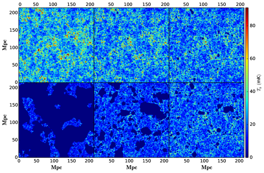
Figure 2: This shows one realization of the two dimensional sections through the simulated H i brightness temperature maps for the $[z,\,\bar{x}_{\rm\text{H\,{i}}}]$ values tabulated in Table 1. In these panels, the value of $\bar{x}_{\rm\text{H\,{i}}}$ decreases in the clockwise direction starting from the top-left panel. Volume of these simulation boxes are $[215\,{\rm Mpc}]^{3}$. These maps are in redshift space, where the line of sight direction is along the vertical axis.

3.2 The Randomized Signal Ensemble (RSE)

We use the Randomized Signal Ensemble (RSE) to interpret the diagonal terms of the error-covariance $\textbf{{C}}_{ij}$ or equivalently the dimensionless error-covariance $\textbf{{c}}_{ij}$. As noted earlier in section 2 we expect $\textbf{{c}}_{ii}=A_{i}^{2}({k_{i}}/{\Delta k_{i}})$ if the EoR 21-cm signal is a Gaussian random field. We interpret any excess relative to this prediction as arising from the trispectrum $t_{ii}$ which arises when the EoR 21-cm signal becomes non-Gaussian. Here we have used logarithmic binning which implies that $(k_{i}/\Delta k_{i})\approx 1.9$ is nearly constant across all the bins. The difficulty is that it is not possible to predict the precise value of $A_{i}$. It is straight forward to see (equation 7) that we have a constant value $A_{i}=1$ if the power spectrum $P(\textbf{{k}})$ has exactly the same value at all the Fourier modes k in the bin. However, this simple assumption is obviously violated, for example redshift space distortion causes the value of $P(\textbf{{k}})$ to vary depending on the direction of k. Further, we have no prior idea of how the simulated EoR power spectrum $P(\textbf{{k}})$ varies across the different Fourier modes within a bin. We have overcome this problem by constructing the RSE as briefly discussed below. The reader is referred to the section 5.1 of Paper I for a detailed discussion on the RSE.

Each realization of the Randomized Signal Ensemble (RSE) is a mixture of Fourier modes $\tilde{T}_{\rm b}(\textbf{{k}})$ drawn from all $50$ realizations of the Signal Ensemble (SE). Considering a particular realization of the RSE, the modes which originate from different realizations of the signal are uncorrelated. This ensures that the trispectrum, which quantifies the correlation between the signal at different Fourier modes, is at least $50$ times smaller for the RSE as compared to the SE. The actual suppression of the trispectrum $t_{ii}$ depends on the number of modes in the $i~{}$th bin, and our earlier studies show that the actual suppression can be considerably more than a factor of $50$ (Figure 5 of Paper I). In this work, we have assumed that $t_{ii}\approx 0$ for the RSE which allows us to interpret $[\textbf{{c}}_{ii}]_{\rm RSE}$ entirely in terms of the power spectrum. Further, the signal is randomized in such a way that we expect both $\bar{P}(k_{i})$ and $\overline{P^{2}}(k_{i})$, and therefore also $A_{i}$ to have exactly the same values for the RSE as compared to the SE. The RSE therefore gives a direct estimate of the error-covariance that would be expected if the trispectrum were zero i.e.

$$[\textbf{{c}}_{ii}]_{\rm RSE}=A_{i}^{2}({k_{i}}/{\Delta k_{i}})\,.$$ (11)

In the subsequent analysis we have used the difference

$$[\textbf{{c}}_{ii}]_{\rm SE}-[\textbf{{c}}_{ii}]_{\rm RSE}=t_{ii}$$ (12)

to directly estimate the reduced trispectrum.

3.3 Ensemble of Gaussian Random Ensembles (EGRE)

We expect the off-diagonal terms of $\textbf{{c}}_{ij}$ to be zero for a Gaussian random field. However, we cannot straightaway interpret the non-zero off-diagonal terms in $\textbf{{c}}_{ij}$ estimated from SE as arising from non-Gaussianity in the EoR 21-cm signal because the SE has a finite number of realizations. To appreciate this we consider a Gaussian Random Ensemble (GRE) which has the same number of realizations of the 21-cm signal as the SE. The off-diagonal terms of the error-covariance $[\textbf{{c}}_{ij}]_{\rm G}$ estimated from GRE will not be zero but will have random fluctuations around zero due to the limited number of realizations. To determine the statistical significance of $\textbf{{c}}_{ij}$, one needs to compare it against the random fluctuation of $[\textbf{{c}}_{ij}]_{\rm G}$. We have used $50$ independent GREs to construct an Ensemble of Gaussian Random Ensembles (EGRE) following the idea presented in Section 5.2 of Paper I. The EGRE has been used to estimate the variance $[\delta\textbf{{c}}_{ij}]_{\rm G}^{2}$ of $[\textbf{{c}}_{ij}]_{\rm G}$. We have compared the estimated $\textbf{{c}}_{ij}$ against $[\delta\textbf{{c}}_{ij}]_{\rm G}$ to determine whether our results are statistically significant or not.

4 Results

Figure 2 shows two dimensional sections through one realization of our simulated three-dimensional 21-cm maps at the redshifts listed in Table 1. We see that the H i very closely follows the underlying dark matter field during the early stages of reionization (top three panels of Figure 2). We expect that the brightness temperature is, to a good approximation, a Gaussian random field at these early stages ($\bar{x}_{\rm\text{H\,{i}}}=0.98,\,0.93$ and $0.86$). However, the non-linearities in the matter density at small scales introduces some amount of non-Gaussianity even during this early phase of reionization. The ‘inside-out’ reionization implemented in these simulations implies that the high-density regions get ionized first and the low-density regions later. Small H ii bubbles located at the high density peaks can be seen even at the early stages. These H ii bubbles grow in both size and in number, and gradually overlap at the later stages of reionization. Finally, at the last stage of reionization we have small islands of H i in an almost completely ionized IGM. In summary, we see that as reionization proceeds the 21-cm signal undergoes a transition from a state where it primarily traces the nearly Gaussian matter fluctuations to a phase where it is nearly entirely determined by a few discrete H i regions which survive to the end of the EoR. We do not show a visualization of the RSE or GRE here, The readers are referred to Figure 1 of Paper I for a visual impression of the RSE and the GRE.

\psfrag{pk}[c][c][1][0]{\large${\Delta^{2}_{\rm b}}\,\,({\rm mK})^{2}$}\psfrag{k}[c][c][1][0]{\large$k\,\,({\rm Mpc}^{-1}$)}\psfrag{10}[c][c][1][0]{\large$10$}\psfrag{0.1}[c][c][1][0]{\large$0.1$}\psfrag{1.0}[c][c][1][0]{\large$1$}\psfrag{z=13, xh1=0.98}[c][c][1][0]{\large$z=13$,\,$\bar{x}_{\rm\text{H\,{i}}}=0.98$\,\,\,\,\,\,\,\,}\psfrag{11, 0.93}[c][c][1][0]{\large$11$,\hskip 31.2982pt$0.93$\,\,\,\,}\psfrag{10, 0.86}[c][c][1][0]{\large$10$,\hskip 31.2982pt$0.86$\,\,\,\,}\psfrag{9, 0.73}[c][c][1][0]{\large$9$,\hskip 31.2982pt\,$0.73$\,\,\,\,}\psfrag{8, 0.50}[c][c][1][0]{\large$8$,\hskip 31.2982pt\,$0.50$\,\,\,\,}\psfrag{7, 0.15}[c][c][1][0]{\large$7$,\hskip 31.2982pt\,$0.15$\,\,\,\,}\includegraphics[width=208.57243pt]{figs/pk.eps}

Figure 3: This shows the mean squared 21-cm brightness temperature fluctuations $\Delta_{\rm b}^{2}(k)$ and its $1\sigma$ error bars (estimated from $50$ different realizations of the simulated signal) for the $[z,\,\bar{x}_{\rm\text{H\,{i}}}]$ values shown in the figure.

Figure 3 shows the mean square brightness temperature fluctuations $\Delta_{\rm b}^{2}(k)=k^{3}\,P(k)/2\pi^{2}$ of the redshifted 21-cm signal as a function of $k$ for the different values of $z$ and $\bar{x}_{\rm\text{H\,{i}}}$ considered here. For each redshift we have estimated the average power spectrum $\bar{P}(k)$ and its $1\sigma$ errors $\delta P(k)=\sqrt{\textbf{{C}}_{ii}}$ using the $50$ statistically independent realizations of SE. We have divided the $k$ range into $10$ equally spaced logarithmic bins for these estimates. We first discuss the power spectrum from the early stages of reionization, i.e. the redshifts $z=13,\,11$ and $10$. During these stages, at large length-scales $k\leq 0.2\,{\rm Mpc}^{-1}$ the shape of the 21-cm power spectrum remains nearly the same as the underlying matter power spectrum. However, the amplitude of $\Delta_{\rm b}^{2}(k)$ slowly decreases as the redshift decreases in contrast to the matter power spectrum whose amplitude increases with decreasing redshift. This is due to the fact that reionization preferentially wipes out the highest density regions in the ‘inside-out’ scenario implemented here. The decrease in the amplitude of the power spectrum is less at small scales where we also notice a steepening of the power spectrum. The decrease in the large-scale amplitude slows down at $z=9$, and we have a reversal in this trend at the lower redshifts. As reionization proceeds from $z=8$ to $7$ the amplitude of the power spectrum increases at large scales $k<0.1\,{\rm Mpc}^{-1}$, however the amplitude decreases at small scales where the power spectrum becomes nearly flat. At these redshifts the turnaround in $\Delta_{\rm b}^{2}(k)$ roughly occurs at a $k$ which corresponds to the radius of the typical ionized regions. Our results here are consistent with several previous studies performed using a variety of different simulation techniques (e.g. McQuinn et al. 2007; Lidz et al. 2008; Barkana 2009; Choudhury et al. 2009; Mesinger et al. 2011; Jensen et al. 2013; Majumdar et al. 2013; Iliev et al. 2014; Majumdar et al. 2016; Dixon et al. 2016 etc.).

\psfrag{cov}[c][c][1][0]{\Large$\textbf{{c}}_{ii}$}\psfrag{k}[c][c][1][0]{\large$k\,\,({\rm Mpc}^{-1})$}\psfrag{SE}[c][c][1][0]{\large SE}\psfrag{RSE}[c][c][1][0]{\large RSE}\psfrag{z=13, xh1=0.98}[c][c][1][0]{\large$z=13$, $\bar{x}_{\rm\text{H\,{i}}}=0.98$}\psfrag{z=11, xh1=0.93}[c][c][1][0]{\large$z=11$, $\bar{x}_{\rm\text{H\,{i}}}=0.93$}\psfrag{z=10, xh1=0.86}[c][c][1][0]{\large$z=10$, $\bar{x}_{\rm\text{H\,{i}}}=0.86$}\psfrag{z=9, xh1=0.73}[c][c][1][0]{\large$z=9$, $\bar{x}_{\rm\text{H\,{i}}}=0.73$}\psfrag{z=8, xh1=0.50}[c][c][1][0]{\large$z=8$, $\bar{x}_{\rm\text{H\,{i}}}=0.50$}\psfrag{z=7, xh1=0.15}[c][c][1][0]{\large$z=7$, $\bar{x}_{\rm\text{H\,{i}}}=0.15$}\psfrag{10}[c][c][1][0]{\large$10$}\psfrag{0.1}[c][c][1][0]{\large$0.1$}\psfrag{1.0}[c][c][1][0]{\large$1$}\psfrag{0.1 1.0}[c][c][1][0]{\large$0.1$\hskip 48.36958pt\,\,\,$1$}\includegraphics[width=440.12402pt]{figs/cov_SE_RSE.eps}

Figure 4: This shows the dimensionless error-variance $\textbf{{c}}_{ii}$ for SE and RSE for the $[z,\,\bar{x}_{\rm\text{H\,{i}}}]$ values shown in the figure.

We next turn our attention to the error-covariance matrix $\textbf{{C}}_{ij}$, and we first consider the diagonal elements which give an estimate of the error-variance $[\delta P(k_{i})]^{2}={\textbf{{C}}_{ii}}$ of the estimated power spectrum. Figure 4 shows the diagonal elements of the dimensionless error-covariance matrix $\textbf{{c}}_{ii}$ defined in equation (5). Here we use $[\textbf{{c}}_{ii}]_{\rm SE}$ to refer to the values which have been estimated from the $50$ realizations of the simulated EoR signal, namely the Signal Ensemble (SE) and we use equation (6) to interpret these results. In addition to this the figure also shows $[\textbf{{c}}_{ii}]_{\rm RSE}$ which (equation 11) gives an estimate of the results that would be expected if the EoR signal were a Gaussian random field with zero trispectrum $t_{ii}=0$. We see (Figure 4) that the values of $[\textbf{{c}}_{ii}]_{\rm RSE}$ are predominantly confined in the range $2$ to $4$ with a maximum value $[\textbf{{c}}_{ii}]_{\rm RSE}\sim 6$ at the largest $k$ bin. In contrast to this, we find that the values of $[\textbf{{c}}_{ii}]_{\rm SE}$ vary over a much wider range with a maximum value $[\textbf{{c}}_{ii}]_{\rm SE}>10^{4}$ at the largest $k$ bin for $\bar{x}_{\rm\text{H\,{i}}}=0.15$. We interpret any difference between $[\textbf{{c}}_{ii}]_{\rm SE}$ and $[\textbf{{c}}_{ii}]_{\rm RSE}$ as arising due to the non-Gaussianity of the EoR 21-cm signal.

We first discuss the results for the highest redshift $z=13$ that we have considered here, shown in the top left panel of Figure 4. It is reasonably valid to assume that at this stage of reionization ($\bar{x}_{\rm\text{H\,{i}}}=0.98$) the H i distribution directly traces the underlying matter. The only non-Gaussianities here are those that arise due to non-linear gravitational clustering of the underlying matter distribution. We see (Figure 4) that the H i signal is consistent with a Gaussian random field at large scales ($k\leq 0.5\,{\rm Mpc}^{-1}$) where $[\textbf{{c}}_{ii}]_{\rm SE}$ is comparable to $[\textbf{{c}}_{ii}]_{\rm RSE}$. The values of $[\textbf{{c}}_{ii}]_{\rm SE}$, however, increase sharply with increasing $k$ for $k>0.5\,{\rm Mpc}^{-1}$ reaching a value $[\textbf{{c}}_{ii}]_{\rm SE}\sim 10^{2}$ at the largest $k$ bin. The H i signal here is non-Gaussian at intermediate and small length-scales ($k>0.5\,{\rm Mpc}^{-1}$) where $[\textbf{{c}}_{ii}]_{\rm SE}$ is larger than $[\textbf{{c}}_{ii}]_{\rm RSE}$. The non-Gaussianity seen here is nearly entirely due to the non-linear gravitational clustering of the underlying matter distribution. The results show a similar behaviour at $z=11$ and $10$.

The effect of non-Gaussianity extends to relatively larger length-scales when the neutral fraction falls to $\bar{x}_{\rm\text{H\,{i}}}=0.73$ at $z=9$ (Figure 4). Here we see that $[\textbf{{c}}_{ii}]_{\rm SE}$ is well in excess of $[\textbf{{c}}_{ii}]_{\rm RSE}$ for $k>0.1\,{\rm Mpc}^{-1}$, and this behaviour possibly extends to even smaller values of $k$ all the way to $k\geq 0.04\,{\rm Mpc}^{-1}$. The behaviour become a little complicated for $\bar{x}_{\rm\text{H\,{i}}}=0.5$ at $z=8$. Here, at small scales the values of $[\textbf{{c}}_{ii}]_{\rm SE}$ increase relative to those at $z=9$, the reverse however is found at intermediate scales $0.1\,<k<1\,{\rm Mpc}^{-1}$. The results, however, are quite unambiguous for $\bar{x}_{\rm\text{H\,{i}}}=0.15$ at $z=7$ where we find that $[\textbf{{c}}_{ii}]_{\rm SE}$ is well in excess of $[\textbf{{c}}_{ii}]_{\rm RSE}$ for $k\geq 0.1\,{\rm Mpc}^{-1}$. Here the value of $[\textbf{{c}}_{ii}]_{\rm SE}$ is found to increase monotonically with increasing $k$, and it has values $\sim 10^{2}$ and $\sim 10^{5}$ at $k\sim 0.5\,{\rm Mpc}^{-1}$ and $k\sim 5.0\,{\rm Mpc}^{-1}$ respectively. We see that the effect of non-Gaussianity becomes particularly important across a wide range of length-scales in the late stages of reionization.

\psfrag{cov}[c][c][1][0]{\Large$\textbf{{c}}_{ii}$}\psfrag{xh1}[c][c][1][0]{\Large$\bar{x}_{\rm HI}$}\psfrag{pk}[c][c][1][0]{\large${\Delta^{2}_{\rm b}}\,\,({\rm mK})^{2}$}\psfrag{SE}[c][c][1][0]{\large SE}\psfrag{RSE}[c][c][1][0]{\large RSE}\psfrag{k=0.12Mpc-1}[c][c][1][0]{\large$k=0.12\,{\rm Mpc}^{-1}$}\psfrag{k=0.57Mpc-1}[c][c][1][0]{\large$k=0.57\,{\rm Mpc}^{-1}$}\psfrag{k=2.75Mpc-1}[c][c][1][0]{\large$k=2.75\,{\rm Mpc}^{-1}$}\psfrag{10}[c][c][1][0]{\large$10$}\psfrag{4}[c][c][1][0]{\large$4$}\psfrag{5}[c][c][1][0]{\large$5$}\psfrag{6}[c][c][1][0]{\large$6$}\psfrag{0.2}[c][c][1][0]{\large$0.2$}\psfrag{0.4}[c][c][1][0]{\large$0.4$}\psfrag{0.6}[c][c][1][0]{\large$0.6$}\psfrag{0.8}[c][c][1][0]{\large$0.8$}\psfrag{1.0}[c][c][1][0]{\large$1$}\includegraphics[width=440.12402pt]{figs/cov_xh1.eps}

Figure 5: This shows the dimensionless error-variance $\textbf{{c}}_{ii}$ for SE as a function of global neutral fraction $\bar{x}_{\rm HI}$ for three representative wave numbers $k=0.12,\,0.57$ and $2.75\,{\rm Mpc^{-1}}$.

Figure 5 shows how $[\textbf{{c}}_{ii}]_{\rm SE}$ and $[\textbf{{c}}_{ii}]_{\rm RSE}$ at three different fixed values of $k$ evolve as a function of $\bar{x}_{\rm\text{H\,{i}}}$. This figure reinforces the findings highlighted in the previous discussion. The values of $\Delta_{\rm b}^{2}(k)$ are also shown in the corresponding top panels for reference. We see that at small $(k=2.75\,{\rm Mpc}^{-1})$ and intermediate $(k=0.57\,{\rm Mpc}^{-1})$ length-scales, the differences between $[\textbf{{c}}_{ii}]_{\rm SE}$ and $[\textbf{{c}}_{ii}]_{\rm RSE}$ are clearly visible over the entire range of evolution ($\bar{x}_{\rm\text{H\,{i}}}=0.98$ to $0.15$) considered here. This implies that at these length-scales the 21-cm signal is significantly non-Gaussian even at the earliest stages of reionization $(\bar{x}_{\rm\text{H\,{i}}}\sim~{}1)$. As mentioned earlier, initially the H i directly traces the underlying matter distribution and the non-Gaussianities here are entirely due to the non-linear gravitational clustering of the underlying matter distribution. As reionization proceeds, it preferentially wipes out the H i in the non-linear high density peaks. At small scales, this causes a drop in the non-Gaussianity of the H i signal in the early stages of reionization, and we see this reflected as a decrement in $[\textbf{{c}}_{ii}]_{\rm SE}$ as $\bar{x}_{\rm\text{H\,{i}}}$ falls from $0.98$ to $0.86$. Subsequently, the value of $[\textbf{{c}}_{ii}]_{\rm SE}$ at small scales increases monotonically by roughly three orders of magnitude as reionization proceeds and the value of $\bar{x}_{\rm\text{H\,{i}}}$ drops from $0.86$ to $0.15$. The non-Gaussianity here is largely dominated by the ionized regions. The behaviour is more complicated at intermediate scales where $[\textbf{{c}}_{ii}]_{\rm SE}$ initially decreases, as reionization proceeds the value of $[\textbf{{c}}_{ii}]_{\rm SE}$ then increases till $\bar{x}_{\rm\text{H\,{i}}}=0.73$, dips again at $\bar{x}_{\rm\text{H\,{i}}}=0.5$ and finally increases at $\bar{x}_{\rm\text{H\,{i}}}=0.15$. At large scales ($k=0.12\,{\rm Mpc}^{-1}$) we find that the values of $[\textbf{{c}}_{ii}]_{\rm SE}$ are comparable to those of $[\textbf{{c}}_{ii}]_{\rm RSE}$ for $\bar{x}_{\rm\text{H\,{i}}}\geq 0.8$ indicating that at large scales the 21-cm signal is consistent with a Gaussian random field in the early stages of reionization. The values of $[\textbf{{c}}_{ii}]_{\rm SE}$ are larger than those of $[\textbf{{c}}_{ii}]_{\rm RSE}$ for $\bar{x}_{\rm\text{H\,{i}}}=0.73$ and $0.15$ indicating that the effect of non-Gaussianity extends to large scales as reionization proceed. However, the value of $[\textbf{{c}}_{ii}]_{\rm SE}$ dips at $\bar{x}_{\rm\text{H\,{i}}}=0.5$ where it is comparable to that of $[\textbf{{c}}_{ii}]_{\rm RSE}$. This behaviour is similar to that seen at intermediate scales where also the non-Gaussianity does not grow monotonically as reionization proceeds but exhibits a dip at $\bar{x}_{\rm\text{H\,{i}}}=0.5$. Note that the peak value $[\textbf{{c}}_{ii}]_{\rm SE}\sim 5$ at large scales is considerably smaller than the peak values of $[\textbf{{c}}_{ii}]_{\rm SE}$ at intermediate or small scales.

\psfrag{k}[c][c][1][0]{\large$k\,\,({\rm Mpc}^{-1})$}\psfrag{cov}[c][c][1][0]{\large$r_{ij}$}\psfrag{ k }[c][c][1][0]{\large$k\,\,({\rm Mpc}^{-1}$)}\includegraphics[width=440.12402pt]{figs/all_cov.eps}

Figure 6: This shows the correlation coefficient $r_{ij}$ estimated from SE for the values of $\bar{x}_{\rm\text{H\,{i}}}$ listed in Table 1. Starting from top-left panel, the value of $\bar{x}_{\rm\text{H\,{i}}}$ decreases clockwise.

We next consider the off-diagonal elements of the error-covariance matrix $\textbf{{C}}_{ij}$. These quantify the correlation between the errors in the power spectrum estimated at different $k$ bins. Following Paper I, we use the dimensionless correlation coefficient

$$r_{ij}=\frac{\textbf{{C}}_{ij}}{\sqrt{\textbf{{C}}_{ii}\,\textbf{{C}}_{jj}}}$$ (13)

to quantify the off-diagonal elements of $\textbf{{C}}_{ij}$. It follows from the definition that $r_{ii}=1$ for all the diagonal elements. The values of $r_{ij}$ lie in the range $-1\leq r_{ij}\leq 1$, the errors in the $i~{}$th and $j~{}$th bins are completely correlated and anti-correlated if $r_{ij}=1$ and $-1$ respectively. The errors in these two bins are uncorrelated if $r_{ij}=0$, and intermediate positive or negative values ($-1<r_{ij}<1$) indicate partial correlations or partial anti-correlations respectively. We expect all the off-diagonal elements to have zero values $(r_{ij}=0)$ if the EoR 21-cm signal is a Gaussian random field.

Figure 6 shows $r_{ij}$ estimated from SE for all the six $z$ and $\bar{x}_{\rm\text{H\,{i}}}$ values listed in Table 1. We see that the errors in the three largest $k$ bins are quite strongly correlated even at the earliest stage $(\bar{x}_{\rm\text{H\,{i}}}=0.98)$. The extent of this correlated region increases at the later stages of reionization. We see that at $\bar{x}_{\rm\text{H\,{i}}}=0.15$ the errors in all the $k$ bins barring the two smallest $k$ values are strongly correlated, the errors in these two smallest $k$ bins are anti-correlated with the errors in all the other bins. It is insightful (see Paper I) to consider Figure 7 where each panel corresponds to a fixed value of $i$ for which it shows $r_{ij}$ as a function of $k_{j}$. Note that in all cases we have $r_{ij}=1$ for the diagonal terms which have $j=i$. Here each horizontal set of panels corresponds to a fixed value of $i$ and each vertical set of panels corresponds to the fixed value of $\bar{x}_{\rm\text{H\,{i}}}$ shown at the top of the figure.

\psfrag{k}[c][c][1][0]{{\large$k\,\,({\rm Mpc}^{-1})$}}\psfrag{cov}[c][c][1][0]{{\Large$r_{ij}$}}\psfrag{z=13, xh1=0.98}[c][c][1][0]{{\large$\bar{x}_{\rm\text{H\,{i}}}=0.98$}}\psfrag{z=11, xh1=0.93}[c][c][1][0]{{\large$\bar{x}_{\rm\text{H\,{i}}}=0.93$}}\psfrag{z=10, xh1=0.86}[c][c][1][0]{{\large$\bar{x}_{\rm\text{H\,{i}}}=0.86$}}\psfrag{z=9, xh1=0.73}[c][c][1][0]{{\large$\bar{x}_{\rm\text{H\,{i}}}=0.73$}}\psfrag{z=8, xh1=0.50}[c][c][1][0]{{\large$\bar{x}_{\rm\text{H\,{i}}}=0.50$}}\psfrag{z=7, xh1=0.15}[c][c][1][0]{{\large$\bar{x}_{\rm\text{H\,{i}}}=0.15$}}\includegraphics[width=420.61192pt]{figs/SE_RSE_EGRE.eps}

Figure 7: This shows $r_{ij}$ estimated from SE (solid) and RSE (dotted). The shaded region represents the $[\delta r_{ij}]_{\rm G}$ which quantifies the $1-\sigma$ fluctuations of the off-diagonal terms around $[r_{ij}]_{\rm G}=0$ expected for a Gaussian random field.

Figure 7 shows the $r_{ij}$ values estimated from SE for all the six $z$ and $\bar{x}_{\rm\text{H\,{i}}}$ values listed in Table 1. Following Paper I, we have used the EGRE (Section 3.3) to estimate $[\delta r_{ij}]_{\rm G}$ which provides an estimate of the fluctuation of the off-diagonal terms around $[r_{ij}]_{\rm G}=0$ expected for a Gaussian random field. We have also shown $r_{ij}$ estimated from RSE (Section 3.2). The RSE has been constructed with the intention of removing any correlation between the signal at different Fourier modes, and we see that the off-diagonal elements of $[r_{ij}]_{\rm RSE}$ are nearly always within the shaded region corresponding to $[\delta r_{ij}]_{\rm G}$.

We first consider the results for $\bar{x}_{\rm\text{H\,{i}}}=0.98$ when the H i essentially traces the underlying matter distribution. We have already seen (Figure 4) that, even at this early stage, the error-variance for the three largest $k$ bins ($k>1.1\,{\rm Mpc}^{-1}$) are significantly in excess of those predicted for a Gaussian random field. Here (Figures 6 and 7) we see that errors in these three $k$ bins are not independent but they are highly correlated. We further see (Figure 7) that the errors in most of the smaller $k$ bins also are correlated with the errors in the three largest $k$ bins. Two of the $k$ bins, $k\approx 0.1\,{\rm Mpc}^{-1}$ and $k\approx 1.0\,{\rm Mpc}^{-1}$, however are exceptions, and the errors in these two $k$ bins are uncorrelated to the errors in any of the other $k$ bins. The results do not change much for $\bar{x}_{\rm\text{H\,{i}}}=0.93$, and we may interpret the results at the two highest $\bar{x}_{\rm\text{H\,{i}}}$ values as reflecting the intrinsic properties of the underlying matter distribution. As mentioned earlier, the evolution of the underlying matter distribution is non-linear at small scales. This introduces non-Gaussianities that not only affect the error estimates at small scales but also causes the errors at large length scales to become correlated with the errors at small scales. The results are somewhat different when the neutral fraction falls further to $\bar{x}_{\rm\text{H\,{i}}}=0.86$, and we may interpret this as the interplay of the intrinsic non-linearities of the underlying matter distribution and the ionization of the H i which preferentially wipes out the 21-cm signal from the most non-linear regions. The extent of the small-scale correlation increases and we now find that the errors in the six largest $k$ bins are correlated. The errors in the two subsequent $k$ bins ($\approx 0.1$ and $0.2\,{\rm Mpc}^{-1}$) are uncorrelated to the errors in any of the other bins, however the errors in the two smallest $k$ bins are correlated with the errors at the largest $k$ bins.

We next discuss the results for $\bar{x}_{\rm\text{H\,{i}}}=0.73$ where the reionization has extended further. Here (Figures 6 and 7) we see that errors in the three largest $k$ bins are strongly correlated among themselves, they are also correlated with the errors in all the other $k$ bins. Interestingly, the errors in even the smallest $k$ bins seem to be weakly correlated among themselves (Figure 7). The results change somewhat for $\bar{x}_{\rm\text{H\,{i}}}=0.5$. The errors at the large $k$ modes again are highly correlated among themselves and also with the errors at the smallest $k$ bins. We have a new feature here that the errors in the two bins with $k\approx 0.07$ and $0.12\,{\rm Mpc}^{-1}$ are anti-correlated with the errors in the two bins with $k\approx 0.34$ and $0.57\,{\rm Mpc}^{-1}$. We note that a similar weak anti-correlation has also been reported earlier in Paper I where the analysis was entirely restricted to $\bar{x}_{\rm\text{H\,{i}}}=0.5$. At the final stages of reionization ($\bar{x}_{\rm\text{H\,{i}}}\approx 0.15$) the errors in nearly all the $k$ bins, barring the two smallest $k$ values, are highly correlated (Figures 6 and 7). The errors in the two smallest $k$ bins are weakly anti-correlated with the errors in all the other $k$ bins. We see (Figure 3) that the 21-cm signal at this last stage of reionization originates from a few surviving low density H i regions. This accounts for the highly correlated errors seen at this stage, however at present we do not have an understanding of the source of the weak anti-correlation seen here.

5 Summary and Discussion

The detection of the EoR 21-cm signal is expected to become a reality with one or many of the current radio interferometers such as LOFAR, MWA and PAPER. It is also anticipated that the first detection would be carried out by measuring the 21-cm power spectrum. The error-covariance of the EoR 21-cm power spectrum is very important for predicting the prospects of a detection with these ongoing experiments. This is also equally important for quantifying the uncertainties in the EoR 21-cm power spectrum once it is measured by any of these experiments. Future instruments such as the SKA and HERA would be able to measure the EoR 21-cm power spectrum with a better precision owing to their enhanced sensitivity. One of their major science goals is to use future high precision measurements to constrain different model parameters of reionization (e.g. Greig & Mesinger 2015; Ewall-Wice et al. 2016). Earlier works which make predictions for different experiments have all assumed that the EoR 21-cm signal is a Gaussian random field. This implies that the error-variance of the 21-cm power spectrum in any $k$ bin depends only on the value of the power spectrum and the number of independent Fourier modes which contribute to the signal in that particular bin. This also implies that the errors in the different $k$ bins are uncorrelated. In our earlier work (Paper I) we have used semi-numerical simulations to analyze the error-covariance matrix $\textbf{{C}}_{ij}$ expected at a particular redshift $z=8$ where the neutral fraction was assumed to have a value $\bar{x}_{\rm\text{H\,{i}}}=0.5$. This reveals that the $\textbf{{C}}_{ij}$ estimated from $50$ independent realizations of the simulated EoR signal shows significant deviations from the predictions of a Gaussian random field. The effect of non-Gaussianity is expected to increase as reionization progresses. In this paper we have extended the analysis of Paper I to cover different stages of reionization.

We find (Figure 4) that even at the very early stage of reionization ($\bar{x}_{\rm\text{H\,{i}}}=0.98$) the dimensionless error-variance $[\textbf{{c}}_{ii}]_{\rm SE}$ is $\sim 2$ – $20$ times larger than the Gaussian prediction $[\textbf{{c}}_{ii}]_{\rm RSE}$ at intermediate and small length-scales ($k>0.5\,{\rm Mpc}^{-1}$). The errors in the three largest $k$ bins ($k>1.5\,{\rm Mpc}^{-1}$) are also highly correlated (Figures 6). The error-variance is consistent with the Gaussian predictions at large length-scales ($k\leq 0.5\,{\rm Mpc}^{-1}$). We however find (Figure 6 and 7) that the errors at large length-scales ($k<0.1\,{\rm Mpc}^{-1}$) and intermediate length-scales ($0.2\leq k\leq 0.6\,{\rm Mpc}^{-1}$) are correlated with the errors in the three largest $k$ bins ($k>1.5\,{\rm Mpc}^{-1}$). As reionization proceeds, the results show a similar behaviour at $\bar{x}_{\rm\text{H\,{i}}}=0.93$. The results are slightly different when the neutral fraction drops to $\bar{x}_{\rm\text{H\,{i}}}=0.86$. The extent of the correlation at small scales now extends to the $6$ largest $k$ bins. The strength of this correlation, however, is slightly weakened compared to the earlier stages of reionization. The error-variance at large length-scales ($k<0.3\,{\rm Mpc}^{-1}$) is consistent with the Gaussian predictions, but these errors still continue to be weakly correlated with the errors in the largest $k$ bins.

As reionization proceeds further we find that the peak value of $[\textbf{{c}}_{ii}]_{\rm SE}$ drops from $\sim 80$ at $\bar{x}_{\rm\text{H\,{i}}}=0.98$ to $\sim 50$ at $\bar{x}_{\rm\text{H\,{i}}}=0.73$. However the length-scales across which the value of $[\textbf{{c}}_{ii}]_{\rm SE}$ exceeds the Gaussian predictions increases to cover the range $k>0.1\,{\rm Mpc}^{-1}$, possibly extending to the smallest $k$ bin $k\geq 0.04\,{\rm Mpc}^{-1}$. The errors in the $3$ largest $k$ bins are highly correlated among themselves, and the errors in all the smaller $k$ bins are also correlated with the errors in the $3$ largest $k$ bins. We however do not find any correlation between the errors at intermediate and large length-scales. The behaviour is a little complicated when the neutral fraction drops to $\bar{x}_{\rm\text{H\,{i}}}=0.5$. At small length scales $k\geq 1.0\,{\rm Mpc}^{-1}$, the value of $[\textbf{{c}}_{ii}]_{\rm SE}$ increases relative to $\bar{x}_{\rm\text{H\,{i}}}=0.73$, with the peak value of $[\textbf{{c}}_{ii}]_{\rm SE}\approx 500$. The errors in the $4$ largest $k$ bins are also highly correlated. The value of $[\textbf{{c}}_{ii}]_{\rm SE}$, however, decreases relative to $\bar{x}_{\rm\text{H\,{i}}}=0.73$ at intermediate length-scales $0.1<k<0.6\,{\rm Mpc}^{-1}$. The errors here are uncorrelated with those in the larger $k$ bins, however they are anti-correlated with the error at $3$ smallest $k$ bins $k<0.2\,{\rm Mpc}^{-1}$. The errors in the smallest $k$ bins ($k<0.2\,{\rm Mpc}^{-1}$) are correlated with those in the $3$ largest $k$ bins ($k>1.0\,{\rm Mpc}^{-1}$) and anticorrelated with the errors at intermediate scales. At the final stage ($\bar{x}_{\rm\text{H\,{i}}}=0.15$) we find that the values of $[\textbf{{c}}_{ii}]_{\rm SE}$ ($\sim 3\times 10^{4}$) increase considerably relative to the earlier stages of reionization, and exceeds the Gaussian predictions in all the bins above $k\geq 0.1\,{\rm Mpc}^{-1}$ (Figure 4). The errors in the large $k$ bins are also highly correlated (Figure 6). The error-variance in the two smallest $k$ bins are consistent with the Gaussian predictions, however the errors here are anti-correlated with the errors in all the larger $k$ bins.

The value of $[\textbf{{c}}_{ii}]_{\rm SE}$ peaks at the largest $k$ bin $(4.66\,{\rm Mpc}^{-1})$ through all stages of reionization. It is interesting to note that this peak value decreases from $\sim 80$ at $\bar{x}_{\rm\text{H\,{i}}}=0.98$ to $\sim 50$ at $\bar{x}_{\rm\text{H\,{i}}}=0.73$ in the early stages of reionization. The peak value subsequently increases sharply to $3\times 10^{4}$ at $\bar{x}_{\rm\text{H\,{i}}}=0.15$. A similar behaviour is seen at $k=2.75\,{\rm Mpc}^{-1}$ (right panel of Figure 5) which is the second largest $k$ bin. In contrast, the value of $[\textbf{{c}}_{ii}]_{\rm SE}$ at the intermediate length-scales $k\sim 0.5\,{\rm Mpc}^{-1}$ initially decreases slightly as $\bar{x}_{\rm\text{H\,{i}}}$ falls from $0.98$ to $0.93$, and then increases to $[\textbf{{c}}_{ii}]_{\rm SE}\sim 10$ at $\bar{x}_{\rm\text{H\,{i}}}=0.73$ (middle panel of Figure 5). The value of $[\textbf{{c}}_{ii}]_{\rm SE}$ subsequently dips to $\sim 3$ for $\bar{x}_{\rm\text{H\,{i}}}=0.5$ and finally increases sharply to $\sim 100$ at $\bar{x}_{\rm\text{H\,{i}}}=0.15$. We find a similar behaviour at large length-scales (left panel of Figure 5). Here the peak values of $[\textbf{{c}}_{ii}]_{\rm SE}$ are in the range $4$ to $5$, and it is not very clear if these are significantly in excess of the Gaussian predictions. It is important to note that even though the error-variance is consistent with the Gaussian predictions at large length-scales, the errors here are correlated with those at smaller length-scales. This clearly indicates that the non-Gaussian effects are important even at the largest length-scales. The analysis of this paper also enables us to estimate the trispectrum of the EoR 21-cm signal $t_{ii}=[\textbf{{c}}_{ii}]_{\rm SE}-[\textbf{{c}}_{ii}]_{\rm RSE}$ (equation 12), however we have not considered this here.

The H i traces the underlying matter distribution during the earliest stage of reionization ($\bar{x}_{\rm\text{H\,{i}}}=0.98$). The non-Gaussianities here arise due to the small scale non-linear gravitational clustering of the underlying matter distribution. We can interpret the excess error-variance at small length-scales as arising from this non-linear gravitational clustering. Further, this also influences large length-scales through mode coupling (Bharadwaj, 1996a, b), and provides an interpretation for the correlation between the errors at large and intermediate length-scales with those at small scales. It is interesting to note that a similar effect is important in the context of galaxy redshift surveys aiming to measure the Baryon Acoustics Oscillations (BAO) where it is found that that the errors at the BAO length-scales ($\sim 150\,{\rm Mpc}$) are influenced by the small scale non-linear gravitational clustering (Hamilton et al., 2006; Neyrinck & Szapudi, 2008; Neyrinck, 2011; Harnois-Déraps & Pen, 2013; Mohammed & Seljak, 2014; Carron et al., 2015).

As reionization proceeds, the H i in the non-linear high density peaks is preferentially ionized in the inside-out reionization scenario implemented in our simulations, resulting in a drop in the non-Gaussianity of the 21-cm signal. At small scales this causes the error-variance to decrease as $\bar{x}_{\rm\text{H\,{i}}}$ falls from $0.98$ to $0.86$. This also causes a weakening of the strength of the correlation between the errors in the different large $k$ bins. In the subsequent two stages of reionization the 21-cm signal is dominated by the discrete ionized bubbles (Figure 2) which have diameters spread around $10-20\,{\rm Mpc}$ and $40-50\,{\rm Mpc}$ for $\bar{x}_{\rm\text{H\,{i}}}=0.73$ and $0.5$ respectively. We expect the Poisson fluctuations from these discrete bubbles to contribute significantly to the non-Gaussianity (Bharadwaj & Pandey, 2005), and we may interpret the excess error-variance here as arising from an interplay between the contribution from the discrete bubbles and the intrinsic non-Gaussianity of the underlying matter distribution. At the final stage ($\bar{x}_{\rm\text{H\,{i}}}=0.15$) the 21-cm signal is dominated by a few discrete surviving H i regions. The excess error-variance and the correlation between the errors here may be interpreted as arising from the Poisson fluctuations due to these discrete H i regions which have sizes in the range $30-50\,{\rm Mpc}$ (Figure 2). At present we do not have an interpretation for the anti-correlation seen at the last two stages of reionization.

Our entire analysis is based on rather simple semi-numerical simulations where the reionization history is determined by three parameters namely $M_{\rm min}$, $N_{\rm ion}$ and $R_{\rm mfp}$ (defined in subsection 3.1). The values of these parameters can be tuned to obtain different reionization histories for which the predicted 21-cm signal also differs. These simulations also do not incorporate X-ray heating (e.g. Ghara et al. 2015; Greig & Mesinger 2015; Mesinger et al. 2016) which will possibly introduce additional non-Gaussianity at the early stages. The predictions will possibly also differ if one includes fully coupled 3D radiative transfer simulations (e.g. Gnedin et al. 2016) or if one considers variations in the reionization sources (e.g. Majumdar et al. 2016). One may question as to how dependent our conclusions are on the parameter values and the method of simulation. To address this issue we have repeated the analysis using the publicly available semi-numerical code 21cmFAST (Mesinger et al., 2011). Like our semi-numerical scheme, 21cmFAST also has three parameters $(T_{\rm vir,min},\,\zeta_{\rm ion},\,R_{\rm mfp})$ which are roughly equivalent to the parameters ($M_{\rm min},N_{\rm ion},R_{\rm mfp}$) used in our simulations. The values of the 21cmFAST parameters were chosen so as to achieve $\bar{x}_{\rm\text{H\,{i}}}=0.5$ at $z=8.0$, and the results were compared with our predictions at $z=8$. The results from 21cmFAST and a detailed comparison with our predictions is presented in Appendix A. To summarize the findings, the 21-cm maps (Figure 8), the power spectrum and the error-variance (Figure 9) are in good agreement at large length-scales ($k\leq 0.2\,{\rm Mpc}^{-1}$). The power spectrum and the error-variance from 21cmFAST exceeds our predictions at larger $k$, the two are however qualitatively similar. In contrast, the correlation between the errors in the different $k$ bins (Figure 10) are quite different for 21cmFAST as compared to our predictions. We see that for 21cmFAST the errors at large length-scales ($k\leq 0.2\,{\rm Mpc}^{-1}$) are strongly anti-correlated with those at small scales ($k\geq 0.3\,{\rm Mpc}^{-1}$), a feature which is not seen in our predictions. In conclusion of this comparison we note that the error predictions presented here do depend on the method and the parameters of the simulation. However, we can definitely treat our predictions as being indicative of the magnitude and the qualitative nature of the deviations from the Gaussian predictions at different stages of reionization. We also note that Majumdar et al. (2014) presents a detailed comparison of the simulation methods implemented in 21cmFAST, our simulations and also a radiative transfer code C²-RAY.

The non-Gaussian nature of the EoR 21-cm signal plays a very significant role in determining the error statistics of the power spectrum, and it is very important to include this when making predictions for ongoing and future experiments. This will also be important for interpreting the results once a detection is made. The various predictions till now have all assumed the EoR 21-cm signal to be a Gaussian random field whereby the power spectrum error-covariance matrix is diagonal and can be easily calculated if the power spectrum is known. In reality, as shown in this work, we expect the error-covariance to be non-diagonal (e.g. Liu et al. 2014a, b) and depend on both the power spectrum and the trispectrum. The most straight forward approach would be to use a statistical ensemble of the simulated 21-cm signal to estimate the error-covariance matrix, as done here, and use this to make more realistic predictions for future and ongoing experiments. It may be noted that we plan to do this in future work. The main difficulty here is that the reionization history and the underlying 21-cm signal are largely unknown. Further, the error predictions also depend on the parameters and the method of simulation. Consequently, the error predictions are inherently uncertain due to the lack of our knowledge of the reionization process and our limited ability to model reionization. However, in all cases we expect the actual error predictions to exceed the Gaussian predictions and we can treat the Gaussian predictions as being upper limits to the signal to noise ratio (SNR) that can be achieved in any experiment. The inclusion of non-Gaussianity will degrade the SNR relative to the Gaussian predictions, the non-Gaussian prediction will however vary with reionization model and method of simulation. The best one can do with the limited understanding of reionization available at present is to have error predictions for different models and simulation methods. With the advent of detections one expects to narrow down the uncertainty in the reionization history and the 21-cm signal. This in turn should lead to better error predictions which should result in a better interpretation of the detection signal.

In future work we plan to use the reionization model and simulation method of this paper to make predictions for ongoing and future EoR experiments including the system noise and other telescope specific effects.

Appendix A Comparison of different models

To test whether our conclusions depend on the parameter values and the method of simulation, we have repeated the analysis using a publicly available semi-numerical code 21cmFAST (Mesinger et al., 2011). The values of the 21cmFAST parameters $(T_{\rm vir,min},\,\zeta_{\rm ion},\,R_{\rm mfp})$ were chosen to be $(3\times 10^{4}\,{\rm K},\,15,\,20\,{\rm Mpc})$ so as to achieve $\bar{x}_{\rm\text{H\,{i}}}=0.5$ at $z=8.0$, and the results were compared with our predictions at a single redshift $z=8$. The spatial resolution $0.56\,{\rm Mpc}$ and the simulation volume $V=[215\,{\rm Mpc}]^{3}$ are maintained the same for both methods.

The two different simulation methods being compared here mainly differ on three counts: (1.) Our method uses a cosmological $N$-body simulation to calculate the matter density field at the desired redshift whereas 21cmFAST uses Zel’dovich approximation (2.) Our method uses FoF to identify the halos which host the ionizing sources whereas 21cmFAST uses a conditional Press-Schechter formalism to calculate the total mass in collapsed halos at every grid point (3.) The particles which represent the H i distribution are displaced along the line of sight to incorporate the effect of peculiar velocities whereas 21cmFAST implements this by multiplying the brightness temperature map with a factor involving the derivative of the radial component of peculiar velocity on a fixed grid without actually moving the H i. Majumdar et al. (2014) presents a detailed comparison of the simulation methods implemented in 21cmFAST and in our simulations.

Figure 8 provides a visual comparison of the H i 21-cm brightness temperature maps for the two different simulation methods. A visual inspection confirms that the maps look roughly similar in nature. However, there are some differences in the ionized bubble sizes and the small scale H i structures. These differences are caused by the differences in the simulation techniques discussed above.

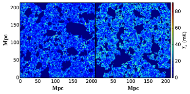
Figure 8: This shows two dimensional sections through H i 21-cm brightness temperature maps simulated using our method (left panel) and 21cmFAST (right panel).

\psfrag{cov}[c][c][1][0]{\small$\textbf{{c}}_{ii}$}\psfrag{pk}[c][c][1][0]{\small${\Delta^{2}_{\rm b}}\,\,({\rm mK})^{2}$}\psfrag{k}[c][c][1][0]{\small$k\,({\rm Mpc}^{-1})$}\includegraphics[width=203.80193pt]{figs/com_pk_cov_SE.eps}

Figure 9: This shows the dimensionless 21-cm brightness temperature fluctuations $\Delta_{\rm b}^{2}(k)$ (left panel) and the dimensionless variance $\textbf{{c}}_{ii}$ as a function of $k$ (right panel). The predictions of our simulation (solid) are compared with those from 21cmFAST (dashed).

We have used $50$ realizations of the 21cmFAST simulations to estimate the mean power spectrum and the error-covariance matrix. The left panel of Figure 9 shows a comparison of $\Delta_{\rm b}^{2}(k)$ calculated using the two different methods. We observe that the power spectrum is in good agreement at large length scales ($k\leq 0.2\,{\rm Mpc}^{-1}$), the results from 21cmFAST are however in excess of our predictions at smaller length scales. The right panel of Figure 9 shows a comparison of the dimensionless error-variance $\textbf{{c}}_{ii}$. Here also we find that the two methods are consistent at large length scales ($k\leq 0.2\,{\rm Mpc}^{-1}$) whereas the results from 21cmFAST are however in excess of our predictions at smaller length scales.

\psfrag{k}[c][c][1][0]{\small$k\,\,({\rm Mpc}^{-1})$}\psfrag{cov}[c][c][1][0]{\small$r_{ij}$}\includegraphics[width=203.80193pt]{figs/com_cov.eps}

Figure 10: This shows the correlation coefficient $r_{ij}$ estimated using our simulations (left panel) and 21cmFAST (right panel).

Figure 10 shows a comparison of the correlation coefficient $r_{ij}$ estimated from the two different methods. We observe that the errors in the largest $k$ bins are strongly correlated for both models. However, the extent of this correlated region is larger for 21cmFAST ($k\geq 0.3\,{\rm Mpc}^{-1}$) as compared to our predictions ($k\geq 1.0\,{\rm Mpc}^{-1}$). We further observe that the errors in the four smallest $k$ bins ($k\leq 0.2\,{\rm Mpc}^{-1}$) are strongly anti-correlated with those at small scales ($k\geq 0.3\,{\rm Mpc}^{-1}$) for 21cmFAST. This feature is not seen in our predictions where the corresponding errors are found to be weakly correlated.

In conclusion of this comparison we note that the error predictions presented here do depend on the method and the parameters of the simulation.

References

- Ali et al. (2008) Ali S. S., Bharadwaj S., Chengalur J. N., 2008, MNRAS, 385, 2166
- Ali et al. (2015) Ali Z. S., et al., 2015, ApJ, 809, 61
- Barkana (2009) Barkana R., 2009, MNRAS, 397, 1454
- Beardsley et al. (2013) Beardsley A. P., et al., 2013, MNRAS, 429, L5
- Becker et al. (2001) Becker R. H., et al., 2001, AJ, 122, 2850
- Becker et al. (2015) Becker G. D., Bolton J. S., Madau P., Pettini M., Ryan-Weber E. V., Venemans B. P., 2015, MNRAS, 447, 3402
- Bernardi et al. (2009) Bernardi G., et al., 2009, A&A, 500, 965
- Bharadwaj (1996a) Bharadwaj S., 1996a, ApJ, 460, 28
- Bharadwaj (1996b) Bharadwaj S., 1996b, ApJ, 472, 1
- Bharadwaj & Pandey (2005) Bharadwaj S., Pandey S. K., 2005, MNRAS, 358, 968
- Bowman et al. (2013) Bowman J. D., et al., 2013, Publ. Astron. Soc. Australia, 30, 31
- Carron et al. (2015) Carron J., Wolk M., Szapudi I., 2015, MNRAS, 453, 450
- Choudhury et al. (2009) Choudhury T. R., Haehnelt M. G., Regan J., 2009, MNRAS, 394, 960
- Davis et al. (1985) Davis M., Efstathiou G., Frenk C. S., White S. D. M., 1985, ApJ, 292, 371
- Dillon et al. (2014) Dillon J. S., et al., 2014, Phys. Rev. D, 89, 023002
- Dixon et al. (2016) Dixon K. L., Iliev I. T., Mellema G., Ahn K., Shapiro P. R., 2016, MNRAS, 456, 3011
- Ewall-Wice et al. (2016) Ewall-Wice A., Hewitt J., Mesinger A., Dillon J. S., Liu A., Pober J., 2016, MNRAS, 458, 2710
- Fan et al. (2003) Fan X., et al., 2003, AJ, 125, 1649
- Furlanetto et al. (2004) Furlanetto S. R., Zaldarriaga M., Hernquist L., 2004, ApJ, 613, 1
- Furlanetto et al. (2009) Furlanetto S. R., et al., 2009, in astro2010: The Astronomy and Astrophysics Decadal Survey. Cosmology from the highly-redshifted 21 cm line, Science White Papers. p. no. 82 (arXiv:0902.3259)
- Ghara et al. (2015) Ghara R., Choudhury T. R., Datta K. K., 2015, MNRAS, 447, 1806
- Ghosh et al. (2012) Ghosh A., Prasad J., Bharadwaj S., Ali S. S., Chengalur J. N., 2012, MNRAS, 426, 3295
- Gnedin et al. (2016) Gnedin N. Y., Becker G. D., Fan X., 2016, preprint, (arXiv:1605.03183)
- Goto et al. (2011) Goto T., Utsumi Y., Hattori T., Miyazaki S., Yamauchi C., 2011, MNRAS, 415, L1
- Greig & Mesinger (2015) Greig B., Mesinger A., 2015, MNRAS, 449, 4246
- Hamilton et al. (2006) Hamilton A. J. S., Rimes C. D., Scoccimarro R., 2006, MNRAS, 371, 1188
- Harnois-Déraps & Pen (2013) Harnois-Déraps J., Pen U.-L., 2013, MNRAS, 431, 3349
- Iliev et al. (2014) Iliev I. T., Mellema G., Ahn K., Shapiro P. R., Mao Y., Pen U.-L., 2014, MNRAS, 439, 725
- Jacobs et al. (2015) Jacobs D. C., et al., 2015, ApJ, 801, 51
- Jensen et al. (2013) Jensen H., et al., 2013, MNRAS, 435, 460
- Komatsu et al. (2011) Komatsu E., et al., 2011, ApJS, 192, 18
- Koopmans et al. (2015) Koopmans L., et al., 2015, Advancing Astrophysics with the Square Kilometre Array (AASKA14), p. 1
- Lidz et al. (2008) Lidz A., Zahn O., McQuinn M., Zaldarriaga M., Hernquist L., 2008, ApJ, 680, 962
- Liu et al. (2014a) Liu A., Parsons A. R., Trott C. M., 2014a, Phys. Rev. D, 90, 023018
- Liu et al. (2014b) Liu A., Parsons A. R., Trott C. M., 2014b, Phys. Rev. D, 90, 023019
- Majumdar et al. (2013) Majumdar S., Bharadwaj S., Choudhury T. R., 2013, MNRAS, 434, 1978
- Majumdar et al. (2014) Majumdar S., Mellema G., Datta K. K., Jensen H., Choudhury T. R., Bharadwaj S., Friedrich M. M., 2014, MNRAS, 443, 2843
- Majumdar et al. (2016) Majumdar S., et al., 2016, MNRAS, 456, 2080
- McQuinn et al. (2006) McQuinn M., Zahn O., Zaldarriaga M., Hernquist L., Furlanetto S. R., 2006, ApJ, 653, 815
- McQuinn et al. (2007) McQuinn M., Lidz A., Zahn O., Dutta S., Hernquist L., Zaldarriaga M., 2007, MNRAS, 377, 1043
- Mellema et al. (2013) Mellema G., et al., 2013, Experimental Astronomy, 36, 235
- Mesinger et al. (2011) Mesinger A., Furlanetto S., Cen R., 2011, MNRAS, 411, 955
- Mesinger et al. (2016) Mesinger A., Greig B., Sobacchi E., 2016, MNRAS, 459, 2342
- Mitra et al. (2011) Mitra S., Choudhury T. R., Ferrara A., 2011, MNRAS, 413, 1569
- Mitra et al. (2013) Mitra S., Ferrara A., Choudhury T. R., 2013, MNRAS, 428, L1
- Mitra et al. (2015) Mitra S., Choudhury T. R., Ferrara A., 2015, MNRAS, 454, L76
- Mohammed & Seljak (2014) Mohammed I., Seljak U., 2014, MNRAS, 445, 3382
- Mondal et al. (2015) Mondal R., Bharadwaj S., Majumdar S., Bera A., Acharyya A., 2015, MNRAS, 449, L41
- Mondal et al. (2016) Mondal R., Bharadwaj S., Majumdar S., 2016, MNRAS, 456, 1936
- Moore et al. (2015) Moore D., et al., 2015, preprint, (arXiv:1502.05072)
- Morales (2005) Morales M. F., 2005, ApJ, 619, 678
- Neyrinck (2011) Neyrinck M. C., 2011, ApJ, 736, 8
- Neyrinck & Szapudi (2008) Neyrinck M. C., Szapudi I., 2008, MNRAS, 384, 1221
- Paciga et al. (2013) Paciga G., et al., 2013, MNRAS, 433, 639
- Parsons et al. (2014) Parsons A. R., et al., 2014, ApJ, 788, 106
- Planck Collaboration et al. (2014) Planck Collaboration et al., 2014, A&A, 571, A16
- Planck Collaboration et al. (2015) Planck Collaboration et al., 2015, preprint, (arXiv:1502.01589)
- Planck Collaboration et al. (2016b) Planck Collaboration et al., 2016b, preprint, (arXiv:1605.02985)
- Planck Collaboration et al. (2016a) Planck Collaboration et al., 2016a, A&A,
- Pober et al. (2013) Pober J. C., et al., 2013, ApJ, 768, L36
- Pober et al. (2014) Pober J. C., et al., 2014, ApJ, 782, 66
- Robertson et al. (2013) Robertson B. E., et al., 2013, ApJ, 768, 71
- Robertson et al. (2015) Robertson B. E., Ellis R. S., Furlanetto S. R., Dunlop J. S., 2015, ApJ, 802, L19
- Songaila & Cowie (2010) Songaila A., Cowie L. L., 2010, ApJ, 721, 1448
- Thomas et al. (2009) Thomas R. M., et al., 2009, MNRAS, 393, 32
- Tingay et al. (2013) Tingay S. J., et al., 2013, Publ. Astron. Soc. Australia, 30, 7
- White et al. (2003) White R. L., Becker R. H., Fan X., Strauss M. A., 2003, AJ, 126, 1
- Yatawatta et al. (2013) Yatawatta S., et al., 2013, A&A, 550, A136
- van Haarlem et al. (2013) van Haarlem M. P., et al., 2013, A&A, 556, A2