Robust Probabilistic Modeling with Bayesian Data Reweighting

Abstract

Probabilistic models analyze data by relying on a set of assumptions. Data that exhibit deviations from these assumptions can undermine inference and prediction quality. Robust models offer protection against mismatch between a model’s assumptions and reality. We propose a way to systematically detect and mitigate mismatch of a large class of probabilistic models. The idea is to raise the likelihood of each observation to a weight and then to infer both the latent variables and the weights from data. Inferring the weights allows a model to identify observations that match its assumptions and down-weight others. This enables robust inference and improves predictive accuracy. We study four different forms of mismatch with reality, ranging from missing latent groups to structure misspecification. A Poisson factorization analysis of the Movielens 1M dataset shows the benefits of this approach in a practical scenario.

1 Introduction

Probabilistic modeling is a powerful approach to discovering hidden patterns in data. We begin by expressing assumptions about the class of patterns we expect to discover; this is how we design a probability model. We follow by inferring the posterior of the model; this is how we discover the specific patterns manifest in an observed data set. Advances in automated inference (hoffman2014nuts; mansinghka2014venture; kucukelbir2016automatic) enable easy development of new models for machine learning and artificial intelligence (ghahramani2015probabilistic).

In this paper, we present a recipe to robustify probabilistic models. What do we mean by “robustify”? Departure from a model’s assumptions can undermine its inference and prediction performance. This can arise due to corrupted observations, or in general, measurements that do not belong to the process we are modeling. Robust models should perform well in spite of such mismatch with reality.

Consider a movie recommendation system. We gather data of people watching movies via the account they use to log in. Imagine a situation where a few observations are corrupted For example, a child logs in to her account and regularly watches popular animated films. One day, her parents use the same account to watch a horror movie. Recommendation models, like Poisson factorization (pf), struggle with this kind of corrupted data (see Section 4): it begins to recommend horror movies.

What can be done to detect and mitigate this effect? One strategy is to design new models that are less sensitive to corrupted data, such as by replacing a Gaussian likelihood with a heavier-tailed $t$ distribution (huber2011robust; insua2012robust). Most probabilistic models we use have more sophisticated structures; these template solutions for specific distributions are not readily applicable. Other classical robust techniques act mostly on distances between observations (huber1973robust); these approaches struggle with high-dimensional data. How can we still make use of our favorite probabilistic models while making them less sensitive to the messy nature of reality?

Main idea. We propose reweighted probabilistic models (rpm). The idea is simple. First, posit a probabilistic model. Then adjust the contribution of each observation by raising each likelihood term to its own (latent) weight. Finally, infer these weights along with the latent variables of the original probability model. The posterior of this adjusted model identifies observations that match its assumptions; it downweights observations that disagree with its assumptions.

Figure 1: Fitting a unimodal distribution to a dataset with corrupted measurements. The rpm downweights the corrupted observations.

Figure 1 depicts this tradeoff. The dataset includes corrupted measurements that undermine the original model; Bayesian data reweighting automatically trades off the low likelihood of the corrupted data near 1.5 to focus on the uncorrupted data near zero. The rpm (green curve) detects this mismatch and mitigates its effect compared to the poor fit of the original model (red curve).

Formally, consider a dataset of $N$ independent observations $y=(y_{1},\ldots,y_{N})$. The likelihood factorizes as a product $\prod_{n=1}^{N}\ell(y_{n}\leavevmode\nobreak\ |\leavevmode\nobreak\ \beta)$, where $\beta$ is a set of latent variables. Posit a prior distribution $p_{\beta}(\beta)$.

Bayesian data reweighting follows three steps:

1. Define a probabilistic model $p_{\beta}(\beta)\prod_{n=1}^{N}\ell(y_{n}\leavevmode\nobreak\ |\leavevmode\nobreak\ \beta)$.

2. Raise each likelihood to a positive latent weight $w_{n}$. Then choose a prior on the weights $p_{w}(w)$, where $w=(w_{1},\ldots,w_{N})$. This gives a reweighted probabilistic model (rpm)

   $$p(y,\beta,w) =\frac{1}{Z}p_{\beta}(\beta)p_{w}(w)\prod_{n=1}^{N}\ell(y_{n}\leavevmode\nobreak\ |\leavevmode\nobreak\ \beta)^{w_{n}},$$

   where $Z$ is the normalizing factor.

3. Infer the posterior of both the latent variables $\beta$ and the weights $w$, $p(\beta,w\leavevmode\nobreak\ |\leavevmode\nobreak\ y)$.

The latent weights $w$ allow an rpm to automatically explore which observations match its assumptions and which do not. Writing out the logarithm of the rpm gives some intuition; it is equal (up to an additive constant) to

$$\log p_{\beta}(\beta)+\log p_{w}(w)+\sum_{n}w_{n}\log\ell(y_{n}\leavevmode\nobreak\ |\leavevmode\nobreak\ \beta).$$ (1)

Posterior inference, loosely speaking, seeks to maximize the above with respect to $\beta$ and $w$. The prior on the weights $p_{w}(w)$ plays a critical role: it trades off extremely low likelihood terms, caused by corrupted measurements, while encouraging the weights to be close to one. We study three options for this prior in Section 2.

How does Bayesian data reweighting induce robustness? First, consider how the weights $w$ affect Equation 1. The logarithm of our priors are dominated by the $\log w_{n}$ term: this is the price of moving $w_{n}$ from one towards zero. By shrinking $w_{n}$, we gain an increase in $w_{n}\log\ell(y_{n}\leavevmode\nobreak\ |\leavevmode\nobreak\ \beta)$ while paying a price in $a\log w_{n}$. The gain outweighs the price we pay if $\log\ell(y_{n}\leavevmode\nobreak\ |\leavevmode\nobreak\ \beta)$ is very negative. Our priors are set to prefer $w_{n}$ to stay close to one; an rpm only shrinks $w_{n}$ for very unlikely (e.g., corrupted) measurements.

Now consider how the latent variables $\beta$ affect Equation 1. As the weights of unlikely measurements shrink, the likelihood term can afford to assign low mass to those corrupted measurements and focus on the rest of the dataset. Jointly, the weights and latent variables work together to automatically identify unlikely measurements and focus on observations that match the original model’s assumptions.

Section 2 presents these intuitions in full detail, along with theoretical corroboration. In Section 3, we study four models under various forms of mismatch with reality, including missing modeling assumptions, misspecified nonlinearities, and skewed data. rpm s provide better parameter inference and improved predictive accuracy across these models. Section 4 presents a recommendation system example, where we improve on predictive performance and identify atypical film enthusiasts in the Movielens 1M dataset.

Related work. Jerzy Neyman elegantly motivates the main idea behind robust probabilistic modeling, a field that has attracted much research attention in the past century.

Every attempt to use mathematics to study some real phenomena must begin with building a mathematical model of these phenomena. Of necessity, the model simplifies matters to a greater or lesser extent and a number of details are ignored. […] The solution of the mathematical problem may be correct and yet it may be in violent conflict with realities simply because the original assumptions of the mathematical model diverge essentially from the conditions of the practical problem considered. (neyman1949problem, p.22).

Our work draws on three themes around robust modeling.

The first is a body of work on robust statistics and machine learning (provost2001robust; song2002robust; NIPS2012_4558; NIPS2014_5428; NIPS2014_5515; NIPS2015_5745). These developments focus on making specific models more robust to imprecise measurements.

One strategy is popular: localization. To localize a probabilistic model, allow each likelihood to depend on its own “copy” of the latent variable $\beta_{n}$. This transforms the model into

$$p(y,\beta,\alpha) =p_{\alpha}(\alpha)\prod_{n=1}^{N}\ell(y_{n}\leavevmode\nobreak\ |\leavevmode\nobreak\ \beta_{n})p_{\beta}(\beta_{n}\leavevmode\nobreak\ |\leavevmode\nobreak\ \alpha),$$ (2)

where a top-level latent variable $\alpha$ ties together all the $\beta_{n}$ variables (deFinetti1961bayesian; wang2015general). Localization decreases the effect of imprecise measurements. rpm s present a broader approach to mitigating mismatch, with improved performance over localization (Sections 3 and 4).

The second theme is robust Bayesian analysis, which studies sensitivity with respect to the prior (berger1994overview). Recent advances directly focus on sensitivity of the posterior (minsker2014robust; miller2015robust) or the posterior predictive distribution (kucukelbir2015population). We draw connections to these ideas throughout this paper.

The third theme is data reweighting. This involves designing individual reweighting schemes for specific tasks and models. Consider robust methods that toss away “outliers.” This strategy involves manually assigning binary weights to datapoints (huber2011robust). Another example is covariate shift adaptation/importance sampling where reweighting transforms data to match another target distribution (veach1995optimally; sugiyama2007covariate; shimodaira2000improving; wen2014robust). A final example is maximum L$q$-likelihood estimation (ferrari2010maximum; qin2013maximum; qin2016robust). Its solutions can be interpreted as a solution to a weighted likelihood, whose weights are proportional to a power transformation of the density. In contrast, rpm s treat weights as latent variables. The weights are automatically inferred; no custom design is required. rpm s also closely connect to ideas around boosting (schapire2012boosting) and variational tempering (mandt2016variational), which also places an exponential weight on the likelihood term. However, they serve different purposes. Boosting reweights to build an ensemble of predictors for supervised learning; variational tempering reweights to escape poor local minima; rpm s reweight to mitigate model mismatch in Bayesian modeling.

2 Reweighted Probabilistic Models

Reweighted probabilistic models (rpm) offer a new approach to robust modeling. The idea is to automatically identify observations that match the assumptions of the model and to base posterior inference on these observations.

2.1 Definitions

An rpm scaffolds over a probabilistic model, $p_{\beta}(\beta)\prod_{n=1}^{N}\ell(y_{n}\leavevmode\nobreak\ |\leavevmode\nobreak\ \beta)$. Raise each likelihood to a latent weight and posit a prior on the weights. This gives the reweighted joint density

$$p(y,\beta,w) =\frac{1}{Z}p_{\beta}(\beta)p_{w}(w)\prod_{n=1}^{N}\ell(y_{n}\leavevmode\nobreak\ |\leavevmode\nobreak\ \beta)^{w_{n}},$$ (3)

where $Z=\int p_{\beta}(\beta)p_{w}(w)\prod_{n=1}^{N}\ell(y_{n}\leavevmode\nobreak\ |\leavevmode\nobreak\ \beta)^{w_{n}}\mathop{}\!\mathrm{d}y\mathop{}\!\mathrm{d}\beta\mathop{}\!\mathrm{d}w$ is the normalizing factor.

The reweighted density integrates to one when the normalizing factor $Z$ is finite. This is always true when the likelihood $\ell(\cdot\leavevmode\nobreak\ |\leavevmode\nobreak\ \beta)$ is an exponential family distribution with Lesbegue base measure (bernardo2009bayesian); this is the class of models we study in this paper.

rpm s apply to likelihoods that factorize over the observations. (We discuss non-exchangeable models in Section 5.) Figure 2 depicts an rpm as a graphical model. Specific models may have additional structure, such as a separation of local and global latent variables (hoffman2013stochastic), or fixed parameters; we omit these in this figure.

(a) Original probabilistic model

(b) Reweighted probabilistic model (rpm)

(c) Localized probabilistic model

Figure 2: rpm s begin with a probabilistic model (a) and introduce a set of weights $w$ as latent variables. This gives a model (b) that explores which data observations match its assumptions. Localization (c), instead, builds a hierarchical model. (Appendix A shows when a localized model is also an rpm.)

The reweighted model introduces a set of weights; these are latent variables, each with support $w_{n}\in\mathbb{R}_{>0}$. To gain intuition, consider how these weights affect the posterior, which is proportional to the product of the likelihood of every measurement. A weight $w_{n}$ that is close to zero flattens out its corresponding likelihood $\ell(y_{n}\leavevmode\nobreak\ |\leavevmode\nobreak\ \beta)^{w_{n}}$; a weight that is larger than one makes its likelihood more peaked. This, in turn, enables the posterior to focus on some measurements more than others. The prior $p_{w}(w)$ ensures that not too many likelihood terms get flattened; in this sense, it plays an important regularization role.

We study three options for this prior on weights: a bank of Beta distributions, a scaled Dirichlet distribution, and a bank of Gamma distributions.

Bank of Beta priors. This option constrains each weight as $w_{n}\in(0,1)$. We posit an independent prior for each weight

$$p_{w}(w) =\prod_{n=1}^{N}\text{Beta}(w_{n}\>;\>a,b)$$ (4)

and use the same parameters $a$ and $b$ for all weights. This is the most conservative option for the rpm; it ensures that none of the likelihoods ever becomes more peaked than it was in the original model.

The parameters $a$, $b$ offer an expressive language to describe different attitudes towards the weights. For example, setting both parameters less than one makes the Beta act like a “two spikes and a slab” prior, encouraging weights to be close to zero or one, but not in between. As another example, setting $a$ greater than $b$ encourages weights to lean towards one.

Scaled Dirichlet prior. This option ensures the sum of the weights equals $N$. We posit a symmetric Dirichlet prior on all the weights

$$\begin{split}w&=Nv\\ p_{v}(v)&=\text{Dirichlet}(a\mathbf{\boldsymbol{1}})\end{split}$$ (5)

where $a$ is a scalar parameter and $\mathbf{\boldsymbol{1}}$ is a $(N\times 1)$ vector of ones. In the original model, where all the weights are one, then the sum of the weights is $N$. The Dirichlet option maintains this balance; while certain likelihoods may become more peaked, others will flatten to compensate.

The concentration parameter $a$ gives an intuitive way to configure the Dirichlet. Small values for $a$ allow the model to easily up- or down-weight many data observations; larger values for $a$ prefer a smoother distribution of weights. The Dirichlet option connects to the bootstrap approaches in rubin1981bayesian; kucukelbir2015population, which also preserves the sum of weights as $N$.

Bank of Gamma priors. Here we posit an independent Gamma prior for each weight

$$p_{w}(w) =\prod_{n=1}^{N}\text{Gamma}(w_{n}\>;\>a,b)$$ (6)

and use the same parameters $a$ and $b$ for all weights. We do not recommend this option, because observations can be arbitrarily up- or down-weighted. In this paper, we only consider Equation 6 for our theoretical analysis in Section 2.2.

The bank of Beta and Dirichlet options perform similarly. We prefer the Beta option as it is more conservative, yet find the Dirichlet to be less sensitive to its parameters. We explore these options in the empirical study (Section 3).

2.2 Theory and intuition

How can theory justify Bayesian data reweighting? Here we investigate its robustness properties. These analyses intend to confirm our intuition from Section 1. Appendices B and C present proofs in full technical detail.

Intuition. Recall the logarithm of the rpm joint density from Equation 1. Now compute the maximum-a-posterior (map) estimate of the weights $w$. The partial derivative is

$$\frac{\partial\log p(y,\beta,w)}{\partial w_{n}} =\frac{\mathop{}\!\mathrm{d}\log p_{w}(w_{n})}{\mathop{}\!\mathrm{d}w_{n}}+\log\ell(y_{n}\leavevmode\nobreak\ |\leavevmode\nobreak\ \beta)$$ (7)

for all $n=1,\ldots,N$. Plug the Gamma prior from Equation 6 into the partial derivative in Equation 7 and set it equal to zero. This gives the map estimate of $w_{n}$,

$$\widehat{w}_{n}=\frac{a-1}{b-\log\ell(y_{n}\leavevmode\nobreak\ |\leavevmode\nobreak\ \beta)}.$$ (8)

The map estimate $\widehat{w}_{n}$ is an increasing function of the log likelihood of $y_{n}$ when $a>1$.This reveals that $\widehat{w}_{n}$ shrinks the contribution of observations that are unlikely under the log likelihood; in turn, this encourages the map estimate for $\widehat{\beta}$ to describe the majority of the observations. This is how an rpm makes a probabilistic model more robust.

A similar argument holds for other exponential family priors on $w$ with $\log w_{n}$ as a sufficient statistic. We formalize this intuition and generalize it in the following theorem, which establishes sufficient conditions where a rpm improves the inference of its latent variables $\beta$.

Theorem 1

Denote the true value of $\beta$ as $\beta^{*}$. Let the posterior mean of $\beta$ under the weighted and unweighted model be $\bar{\beta}_{w}$ and $\bar{\beta}_{u}$ respectively. Assume mild conditions on $p_{w}$, $\ell$ and the corruption level, and that $|\ell(y_{n}\leavevmode\nobreak\ |\leavevmode\nobreak\ \bar{\beta}_{w})-\ell(y_{n}\leavevmode\nobreak\ |\leavevmode\nobreak\ \beta^{*})|<\epsilon$ holds $\forall n$ with high probability. Then, there exists an $N^{*}$ such that for $N>N^{*}$, we have $|\bar{\beta}_{u}-\beta^{*}|\succeq_{2}|\bar{\beta}_{w}-\beta^{*}|$, where $\succeq_{2}$ denotes second order stochastic dominance. (Details in Appendix B.)

The likelihood bounding assumption is common in robust statistics theory; it is satisfied for both likely and unlikely (corrupted) measurements. How much of an improvement does it give? We can quantify this through the influence function (if) of $\bar{\beta}_{w}$.

Consider a distribution $G$ and a statistic $T(G)$ to be a function of data that comes iid from $G$. Take a fixed distribution, e.g., the population distribution, $F$. Then, if $(z;T,F)$ measures how much an additional observation at $z$ affects the statistic $T(F)$. Define

$$\textsc{if}(z;T,F) =\lim_{t\rightarrow 0^{+}}\frac{T(t\delta_{z}+(1-t)F)-T(F)}{t}$$

for $z$ where this limit exists. Roughly, the if measures the asymptotic bias on $T(F)$ caused by a specific observation $z$ that does not come from $F$. We consider a statistic $T$ to be robust if its if is a bounded function of $z$, i.e., if outliers can only exert a limited influence (huber2011robust).

Here, we study the if of the posterior mean $T=\bar{\beta}_{w}$ under the true data generating distribution $F=\ell(\cdot\leavevmode\nobreak\ |\leavevmode\nobreak\ \beta^{*})$. Say a value $z$ has likelihood $\ell(z\leavevmode\nobreak\ |\leavevmode\nobreak\ \beta^{*})$ that is nearly zero; we think of this $z$ as corrupted. Now consider the weight function induced by the prior $p_{w}(w)$. Rewrite it as a function of the log likelihood, like $w(\log\ell(\cdot\leavevmode\nobreak\ |\leavevmode\nobreak\ \beta^{*}))$ as in Equation 8.

Theorem 2

If $\lim_{a\rightarrow-\infty}w(a)=0$ and $\lim_{a\rightarrow-\infty}a\cdot w(a)<\infty$, then $\textsc{if}(z;\bar{\beta}_{w},\ell(\cdot\leavevmode\nobreak\ |\leavevmode\nobreak\ \beta^{*}))\rightarrow 0\text{ as }\ell(z\leavevmode\nobreak\ |\leavevmode\nobreak\ \beta^{*})\rightarrow 0.$

This result shows that an rpm is robust in that its if goes to zero for unlikely measurements. This is true for all three priors. (Details in Appendix C.)

2.3 Inference and computation

We now turn to inferring the posterior of an rpm, $p(\beta,w\leavevmode\nobreak\ |\leavevmode\nobreak\ y)$. The posterior lacks an analytic closed-form expression for all but the simplest of models; even if the original model admits such a posterior for $\beta$, the reweighted posterior may take a different form.

To approximate the posterior, we appeal to probabilistic programming. A probabilistic programming system enables a user to write a probability model as a computer program and then compile that program into an inference executable. Automated inference is the backbone of such systems: it takes in a probability model, expressed as a program, and outputs an efficient algorithm for inference. We use automated inference in Stan, a probabilistic programming system (carpenter2015stan).

In the empirical study that follows, we highlight how rpm s detect and mitigate various forms of model mismatch. As a common metric, we compare the predictive accuracy on held out data for the original, localized, and reweighted model.

The posterior predictive likelihood of a new datapoint $y_{\dagger}$ is $p_{\text{original}}(y_{\dagger}\leavevmode\nobreak\ |\leavevmode\nobreak\ y)=\int\ell(y_{\dagger}\leavevmode\nobreak\ |\leavevmode\nobreak\ \beta)p(\beta\leavevmode\nobreak\ |\leavevmode\nobreak\ y)\mathop{}\!\mathrm{d}\beta.$ Localization couples each observation with its own copy of the latent variable; this gives $p_{\text{localized}}(y_{\dagger}\leavevmode\nobreak\ |\leavevmode\nobreak\ y)=\iint\!\ell(y_{\dagger}\leavevmode\nobreak\ |\leavevmode\nobreak\ \beta_{\dagger})p(\beta_{\dagger}\leavevmode\nobreak\ |\leavevmode\nobreak\ \alpha)p(\alpha\leavevmode\nobreak\ |\leavevmode\nobreak\ y)\mathop{}\!\mathrm{d}\alpha\mathop{}\!\mathrm{d}\beta_{\dagger}$ where $\beta_{\dagger}$ is the localized latent variable for the new datapoint. The prior $p(\beta_{\dagger}\leavevmode\nobreak\ |\leavevmode\nobreak\ \alpha)$ has the same form as $p_{\beta}$ in Equation 2.

Bayesian data reweighting gives the following posterior predictive likelihood

$$p_{\textsc{rpm}}(y_{\dagger}\leavevmode\nobreak\ |\leavevmode\nobreak\ y) =\iint\!p(y_{\dagger}\leavevmode\nobreak\ |\leavevmode\nobreak\ \beta,w_{\dagger})p_{\textsc{rpm}}(\beta\leavevmode\nobreak\ |\leavevmode\nobreak\ y)p(w_{\dagger})\>\mathop{}\!\mathrm{d}w_{\dagger}\mathop{}\!\mathrm{d}\beta,$$

where $p_{\textsc{rpm}}(\beta\leavevmode\nobreak\ |\leavevmode\nobreak\ y)$ is the marginal posterior, integrating out the inferred weights of the training dataset, and the prior $p(w_{\dagger})$ has the same form as $p_{w}$ in Equation 3.

3 Empirical Study

We study rpm s under four types of mismatch with reality. This section involves simulations of realistic scenarios; the next section presents a recommendation system example using real data. We default to No-U-Turn sampler (nuts) (hoffman2014nuts) for inference in all experiments, except for Sections 3.5 and 4 where we leverage variational inference (kucukelbir2016automatic). The additional computational cost of inferring the weights is unnoticeable relative to inference in the original model.

3.1 Outliers: a network wait-time example

A router receives packets over a network and measures the time it waits for each packet. Suppose we typically observe wait-times that follow a Poisson distribution with rate $\beta=5$. We model each measurement using a Poisson likelihood $\ell(y_{n}\leavevmode\nobreak\ |\leavevmode\nobreak\ \beta)=\text{Poisson}(\beta)$ and posit a Gamma prior on the rate $p_{\beta}(\beta)=\textrm{Gam}(a=2,b=0.5)$.

Imagine that $F$% percent of the time, the network fails. During these failures, the wait-times come from a Poisson with much higher rate $\beta=50$. Thus, the data actually contains a mixture of two Poisson distributions; yet, our model only assumes one. (Details in Section D.1.)

(a) Posteriors for $F=25\%$ failure rate.

(b) Posterior 95% credible intervals.

Figure 3: Outliers simulation study. We compare $\text{Beta}(0.1,0.01)$ and $\text{Dir}(\mathbf{\boldsymbol{1}})$ as priors for the reweighted probabilistic model. (a) Posterior distributions on $\beta$ show a marked difference in detecting the correct wait-time rate of $\beta=5$. (b) Posterior 95% confidence intervals across failure rates $F$ show consistent behavior for both Beta and Dirichlet priors. ($N=100$ with 50 replications.)

How do we expect an rpm to behave in this situation? Suppose the network failed 25% of the time. Figure 3(a) shows the posterior distribution on the rate $\beta$. The original posterior is centered at 18; this is troubling, not only because the rate is wrong but also because of how confident the posterior fit is. Localization introduces greater uncertainty, yet still estimates a rate around 15. The rpm correctly identifies that the majority of the observations come from $\beta=5$. Observations from when the network failed are down-weighted. It gives a confident posterior centered at five.

Figure 3(b) shows posterior 95% credible intervals of $\beta$ under failure rates up to $F=45\%$. The rpm is robust to corrupted measurements; instead it focuses on data that it can explain within its assumptions. When there is no corruption, the rpm performs just as well as the original model.

Visualizing the weights elucidates this point. Figure 4 shows the posterior mean estimates of $w$ for $F=25\%$. The weights are sorted into two groups, for ease of viewing. The weights of the corrupted observations are essentially zero; this downweighting is what allows the rpm to shift its posterior on $\beta$ towards five.

Figure 4: Posterior means of the weights $w$ under the Dirichlet prior. For visualization purposes, we sorted the data into two groups: the first 75 contain observations from the normal network; the remaining 25 are the observations when the network fails.

Despite this downweighting, the rpm posteriors on $\beta$ are not overdispersed, as in the localized case. This is due to the interplay we described in the introduction. Downweighting observations should lead to a smaller effective sample size, which would increase posterior uncertainty. But the downweighted datapoints are corrupted observations; including them also increases posterior uncertainty.

The rpm is insensitive to the prior on the weights; both Beta and Dirichlet options perform similarly. From here on, we focus on the Beta option. We let the shape parameter $a$ scale with the data size $N$ such that $N/a\approx 10^{3}$; this encodes a mild attitude towards unit weights. We now move on to other forms of mismatch with reality.

3.2 Missing latent groups: predicting color blindness

Color blindness is unevenly hereditary: it is much higher for men than for women (boron2012medical). Suppose we are not aware of this fact. We have a dataset of both genders with each individual’s color blindness status and his/her relevant family history. No gender information is available. Consider analyzing this data using logistic regression. It can only capture one hereditary group. Thus, logistic regression misrepresents both groups, even though men exhibit strong heredity. In contrast, an rpm can detect and mitigate the missing group effect by focusing on the dominant hereditary trait. Here we consider men as the dominant group.

We simulate this scenario by drawing binary indicators of color blindness $y_{n}\sim\text{Bernoulli}(1/1+\exp(-p_{n}))$ where the $p_{n}$’s come from two latent groups: men exhibit a stronger dependency on family history ($p_{n}=0.5x_{n}$) than women ($p_{n}=0.01x_{n}$). We simulate family history as $x_{n}\sim\text{Unif}(-10,10)$. Consider a Bayesian logistic regression model without intercept. Posit a prior on the slope as $p_{\beta}(\beta)=\mathcal{N}(0,10)$ and assume a $\text{Beta}(0.1,0.01)$ prior on the weights. (Details in Section D.2.)

Figure 5: Missing latent groups study. Posterior 95% credible intervals for the rpm always include the dominant $\beta_{\text{men}}=0.5$, as we vary the percentage of females in the data. Dataset size $N=100$ with $50$ replications.

Figure 5 shows the posterior 95% credible intervals of $\beta$ as we vary the percentage of females from $F=0\%$ to 40%. A horizontal line indicates the correct slope for the dominant group, $\beta_{\text{men}}=0.5$. As the size of the missing latent group (women) increases, the original model quickly shifts its credible interval away from $0.5$. The reweighted and localized posteriors both contain $\beta_{\text{men}}=0.5$ for all percentages, but the localized model exhibits much higher variance in its estimates.

True structure	Model structure	Original	rpm	Localization
		mean(std)	mean(std)	mean(std)
$\beta_{0}+\beta_{1}x_{1}+\beta_{2}x_{2}+\beta_{3}x_{1}x_{2}$	$\beta_{0}+\beta_{1}x_{1}+\beta_{2}x_{2}$	3.16(1.37)	2.20(1.25)	2.63(1.85)
$\beta_{0}+\beta_{1}x_{1}+\beta_{2}x_{2}+\beta_{3}x_{2}^{2}$	$\beta_{0}+\beta_{1}x_{1}+\beta_{2}x_{2}$	30.79(2.60)	16.32(1.96)	21.08(5.20)
$\beta_{0}+\beta_{1}x_{1}+\beta_{2}x_{2}$	$\beta_{0}+\beta_{1}x_{1}$	0.58(0.38)	0.60(0.40)	0.98(0.54)

Table 1: rpm s improve absolute deviations of posterior mean $\beta_{1}$ estimates. (50 replications.)

This analysis shows how rpm s can mitigate the effect of missing latent groups. While the original logistic regression model would perform equally poorly on both groups, an rpm is able to automatically focus on the dominant group.

Figure 6: Kernel density estimate of the distribution of weights across all measurements in the missing latent groups study. The percentage of females is denoted by $F$. A hypothetical clean dataset receives weights that concentrate around one; the actual corrupted dataset exhibits a two-hump distribution of weights.

An rpm also functions as a diagnostic tool to detect mismatch with reality. The distribution of the inferred weights indicates the presence of datapoints that defy the assumptions of the original model. Figure 6 shows a kernel density estimate of the inferred posterior weights. A hypothetical dataset with no corrupted measurements receives weights close to one. In contrast, the actual dataset with measurements from a missing latent group exhibit a bimodal distribution of weights. Testing for bimodality of the inferred weights is one way in which an rpm can be used to diagnose mismatch with reality.

3.3 Covariate dependence misspecification: a lung cancer risk study

Consider a study of lung cancer risk. While tobacco usage exhibits a clear connection, other factors may also contribute. For instance, obesity and tobacco usage appear to interact, with evidence towards a quadratic dependence on obesity (odegaard2010bmi).

Denote tobacco usage as $x_{1}$ and obesity as $x_{2}$. We study three models of lung cancer risk dependency on these covariates. We are primarily interested in understanding the effect of tobacco usage; thus we focus on $\beta_{1}$, the regression coefficient for tobacco. In each model, some form of covariance misspecification discriminates the true structure from the assumed structure.

For each model, we simulate a dataset of size $N=100$ with random covariates $x_{1}\sim\mathcal{N}(10,5^{2})$ and $x_{2}\sim\mathcal{N}(0,10^{2})$ and regression coefficients $\beta_{0,1,2,3}\sim\text{Unif}(-10,10)$. Consider a Bayesian linear regression model with prior $p_{\beta}(\beta)=\mathcal{N}(0,10)$. (Details in Section D.3.)

Table 1 summarizes the misspecification and shows absolute differences on the estimated ${\beta}_{1}$ regression coefficient. The rpm yields better estimates of $\beta_{1}$ in the first two models. These highlight how the rpm leverages datapoints useful for estimating $\beta_{1}$. The third model is particularly challenging because obesity is ignored in the misspecified model. Here, the rpm gives similar results to the original model; this highlights that rpm s can only use available information. Since the original model lacks dependence on $x_{2}$, the rpm cannot compensate for this.

	Outliers		Missing latent groups		Misspecified structure
	Clean	Corrupted	Clean	Corrupted	Clean	Corrupted
Original model	$-744.2$	$-1244.5$	$-108.6$	$-103.9$	$-136.3$	$-161.7$
Localized model	$-730.8$	$-1258.4$	$-53.6$	$-112.7$	$-192.5$	$-193.1$
rpm	$-328.5$	$-1146.9$	$-43.9$	$-90.5$	$-124.1$	$-144.1$

Table 2: Posterior predictive likelihoods of clean and corrupted test data. Outliers and missing latent groups have $F=25\%$. The misspecified structure is missing the interaction term. Results are similar for other levels and types of mismatch with reality.

3.4 Predictive likelihood results

Table 2 shows how rpm s also improve predictive accuracy. In all the above examples, we simulate test data with and without their respective types of corruption. rpm s improve prediction for both clean and corrupted data, as they focus on data that match the assumptions of the original model.

3.5 Skewed data: cluster selection in a mixture model

Finally, we show how rpm s handle skewed data. The Dirichlet process mixture model (dpmm) is a versatile model for density estimation and clustering (bishop2006pattern; murphy2012machine). While real data may indeed come from a finite mixture of clusters, there is no reason to assume each cluster is distributed as a Gaussian. Inspired by the experiments in miller2015robust, we show how a reweighted dpmm reliably recovers the correct number of components in a mixture of skewnormals dataset.

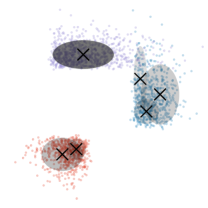
(a) Original model

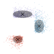
(b) rpm

Figure 7: A finite approximation dpmm to skewnormal distributed data that come from three groups. The shade of each cluster indicates the inferred mixture proportions ($N=2000$).

A standard Gaussian mixture model (gmm) with large $K$ and a sparse Dirichlet prior on the mixture proportions is an approximation to a dpmm (ishwaran2012approximate). We simulate three clusters from two-dimensional skewnormal distributions and fit a gmm with maximum $K=30$. Here we use automatic differentiation variational inference (advi), as nuts struggles with inference of mixture models (kucukelbir2016automatic). (Details in Section D.4.)

Figure 7 shows posterior mean estimates from the original gmm; it incorrectly finds six clusters. In contrast, the rpm identifies the correct three clusters. Datapoints in the tails of each cluster get down-weighted; these are datapoints that do not match the Gaussianity assumption of the model.

4 Case Study: Poisson factorization for recommendation

We now turn to a study of real data: a recommendation system. Consider a video streaming service; data comes as a binary matrix of users and the movies they choose to watch. How can we identify patterns from such data? Poisson factorization (pf) offers a flexible solution (cemgil2009bayesian; gopalan2015scalable). The idea is to infer a $K$-dimensional latent space of user preferences $\mathbf{\boldsymbol{\theta}}$ and movie attributes $\mathbf{\boldsymbol{\beta}}$. The inner product $\mathbf{\boldsymbol{\theta}}^{\top}\mathbf{\boldsymbol{\beta}}$ determines the rate of a Poisson likelihood for each binary measurement; Gamma priors on $\mathbf{\boldsymbol{\theta}}$ and $\mathbf{\boldsymbol{\beta}}$ promote sparse patterns. As a result, pf finds interpretable groupings of movies, often clustered according to popularity or genre. (Full model in Appendix E.)

How does classical pf compare to its reweighted counterpart? As input, we use the MovieLens 1M dataset, which contains one million movie ratings from $6\,000$ users on $4\,000$ movies. We place iid $\text{Gamma}(1,0.001)$ priors on the preferences and attributes. Here, we have the option of reweighting users or items. We focus on users and place a $\text{Beta}(100,1)$ prior on their weights. For this model, we use map estimation. (Localization is computationally challenging for pf; it requires a separate “copy” of $\mathbf{\boldsymbol{\theta}}$ for each movie, along with a separate $\mathbf{\boldsymbol{\beta}}$ for each user. This dramatically increases computational cost.)

(a) Original dataset

(b) Corrupted users

Figure 8: Inferred weights for clean and corrupted data. (a) Most users receive weights very close to one. (b) Corrupted users receive weights much smaller than one. Larger ratios of corruption $R$ imply lower weights.

Average log likelihood	Corrupted users
	0%	1%	2%
Original model	$-1.68$	$-1.73$	$-1.74$
rpm	$\mathbf{\boldsymbol{-1.53}}$	$\mathbf{\boldsymbol{-1.53}}$	$\mathbf{\boldsymbol{-1.52}}$

Table 3: Held-out predictive accuracy under varying amounts of corruption. Held-out users chosen randomly ($20\%$ of total users).

We begin by analyzing the original (clean) dataset. Reweighting improves the average held-out log likelihood from $-1.68$ of the original model to $-1.53$ of the corresponding rpm. The boxplot in Figure 8(a) shows the inferred weights. The majority of users receive weight one, but a few users are down-weighted. These are film enthusiasts who appear to indiscriminately watch many movies from many genres. (Appendix F shows an example.) These users do not contribute towards identifying movies that go together; this explains why the rpm down-weights them.

Recall the example from our introduction. A child typically watches popular animated films, but her parents occasionally use her account to watch horror films. We simulate this by corrupting a small percentage of users. We replace a ratio $R=(0.1,0.5,1)$ of these users’ movies with randomly selected movies.

The boxplot in Figure 8(b) shows the weights we infer for these corrupted users, based on how many of their movies we randomly replace. The weights decrease as we corrupt more movies. Table 3 shows how this leads to higher held-out predictive accuracy; down-weighting these corrupted users leads to better prediction.

5 Discussion

Reweighted probabilistic models (rpm) offer a systematic approach to mitigating various forms of mismatch with reality. The idea is to raise each data likelihood to a weight and to infer the weights along with the hidden patterns. We demonstrate how this strategy introduces robustness and improves prediction accuracy across four types of mismatch.

rpm s also offer a way to detect mismatch with reality. The distribution of the inferred weights sheds light onto datapoints that fail to match the original model’s assumptions. rpm s can thus lead to new model development and deeper insights about our data.

rpm s can also work with non-exchangeable data, such as time series. Some time series models admit exchangeable likelihood approximations (guinness2013transformation). For other models, a non-overlapping windowing approach would also work. The idea of reweighting could also extend to structured likelihoods, such as Hawkes process models.

Appendix A Localized generalized linear model as an rpm

Localization in generalized linear models (glms) is equivalent to reweighting, with constraints on the weight function $w(\cdot)$ induced by $p_{w}$. We prelude the theorem with a simple illustration in linear regression.

Consider $N$ iid observations $\{(x_{n},y_{n})\}^{N}_{1}$. We regress $y$ against $x$:

$$y_{n}=\beta_{1}(x_{n}-\bar{x})+\beta_{0}+\epsilon_{n},\epsilon_{n}\stackrel{{\scriptstyle iid}}{{\sim}}N(0,\sigma^{2}),$$

where $\bar{x}=\sum^{N}_{n=1}x_{n}$. The maximum likelihood estimate of $(\beta_{0},\beta_{1})$ is

$$(\widehat{\beta}_{0},\widehat{\beta}_{1})=\text{argmin}_{\beta_{0},\beta_{1}}\sum^{N}_{n=1}(y_{n}-\beta_{1}(x_{n}-\bar{x})-\beta_{0})^{2}.$$

The localized model is

$$y_{n}=\beta_{1n}\times(x_{n}-\bar{x})+\beta_{0}+\epsilon_{n},\beta_{1n}\stackrel{{\scriptstyle iid}}{{\sim}}N(\beta_{1},\lambda^{2}),\epsilon_{n}\stackrel{{\scriptstyle iid}}{{\sim}}N(0,\sigma^{2}),$$

where $\{\beta_{1n}\}^{N}_{n=1}\mathchoice{\mathrel{\hbox to0.0pt{$\displaystyle\perp$\hss}\mkern 2.0mu{\displaystyle\perp}}}{\mathrel{\hbox to0.0pt{$\textstyle\perp$\hss}\mkern 2.0mu{\textstyle\perp}}}{\mathrel{\hbox to0.0pt{$\scriptstyle\perp$\hss}\mkern 2.0mu{\scriptstyle\perp}}}{\mathrel{\hbox to0.0pt{$\scriptscriptstyle\perp$\hss}\mkern 2.0mu{\scriptscriptstyle\perp}}}\{\epsilon_{n}\}^{N}_{n=1}$. Marginalizing out $\beta_{1n}$’s gives

$$y_{n}=\beta_{1}\times(x_{n}-\bar{x})+\beta_{0}+\gamma_{n},\gamma_{n}\stackrel{{\scriptstyle iid}}{{\sim}}N(0,(x_{n}-\bar{x})^{2}\cdot\lambda^{2}+\sigma^{2}).$$

The maximum likelihood estimate of $(\beta_{0},\beta_{1})$ in the localized model thus becomes

$$(\widehat{\beta}_{0},\widehat{\beta}_{1})=\text{argmin}_{\beta_{0},\beta_{1}}\sum^{N}_{n=1}\frac{(y_{n}-\beta_{1}(x_{n}-\bar{x})-\beta_{0})^{2}}{(x_{n}-\bar{x})^{2}\cdot\lambda^{2}+\sigma^{2}}.$$

This is equivalent to the reweighting approach with

$$w_{n}=\frac{1}{(x_{n}-\bar{x})^{2}\cdot\lambda^{2}+\sigma^{2}}.$$

We generalize this argument into generalized linear models.

Theorem 3

Localization in a glm with identity link infers $\beta_{1}$ from

$$y_{n}\leavevmode\nobreak\ |\leavevmode\nobreak\ x_{n},\beta_{1n},\beta_{0} \sim\exp\left(\frac{y_{n}\cdot\eta_{n}-b_{1}(\eta_{n})}{a_{1}(\phi)}+c_{1}(y_{n},\phi)\right),$$

$$\eta_{n} =\beta_{0}+\beta_{1n}\cdot(x_{n}-\bar{x}),$$

$$\beta_{1n}\leavevmode\nobreak\ |\leavevmode\nobreak\ \beta_{1} \sim\exp\left(\frac{\beta_{1n}\cdot\beta_{1}-b_{2}(\beta_{1})}{a_{2}(\nu)}+c_{2}(\beta_{1n},\nu)\right),$$

where $a_{1}(\cdot),a_{2}(\cdot)$ denote dispersion constants, $b_{1}(\cdot),b_{2}(\cdot)$ denote normalizing constants, and $c_{1}(\cdot),c_{2}(\cdot)$ denote carrier densities of exponential family distributions.

Inferring $\beta_{1}$ from this localized glm is equivalent to inferring $\beta_{1}$ from the reweighted model with weights

$$w_{n} =\mathbb{E}_{p(\beta_{1n}|\beta_{1})}\left[\exp\left(\frac{(y_{n}-E(y_{n}\leavevmode\nobreak\ |\leavevmode\nobreak\ \beta_{0}+\tilde{\beta}_{1n}(x_{n}-\bar{x})))(\beta_{1n}-\beta_{1})(x_{n}-\bar{x})}{a_{1}(\phi)}\right)\right]$$

for some $\{\tilde{\beta}_{1n}\}^{N}_{1}$.

Proof A classical glm with an identity link is

$$y_{n}\sim\exp\left(\frac{y_{n}\cdot\eta_{n}-b_{1}(\eta_{n})}{a_{1}(\phi)}+c_{1}(y_{n},\phi)\right),$$

$$\eta_{n}=\beta_{0}+\beta_{1}\cdot(x_{n}-\bar{x}),$$

whose maximum likelihood estimate calculates

$$(\widehat{\beta}_{0},\widehat{\beta}_{1})=\text{argmax}_{\beta_{0},\beta_{1}}\prod^{N}_{n=1}L_{c,n},$$

where

$$L_{c,n}=\exp\left(\frac{y_{n}\cdot(\beta_{0}+\beta_{1}(x_{n}-\bar{x}))-b_{1}(\beta_{0}+\beta_{1}(x_{n}-\bar{x}))}{a_{1}(\phi)}+c_{1}(y_{n},\phi)\right).$$

On the other hand, the maximum likelihood estimate of the localized model calculates

$$(\widehat{\beta}_{0},\widehat{\beta}_{1})=\text{argmax}_{\beta_{0},\beta_{1}}\prod^{N}_{n=1}L_{l,n},$$

where

$$L_{l,n}=\int\exp\left(\frac{y_{n}\cdot(\beta_{0}+\beta_{1n}(x_{n}-\bar{x}))-b_{1}(\beta_{0}+\beta_{1n}(x_{n}-\bar{x}))}{a_{1}(\phi)}+c_{1}(y_{n},\phi)\right.$$

$$\left.+\frac{\beta_{1n}\beta_{1}-b_{2}(\beta_{1})}{a_{2}(\nu)}+c_{2}(\beta_{1n},\nu)\right)d\beta_{1n}.$$

A localized glm is thus reweighting the likelihood term of each observation by

$$\frac{L_{l,n}}{L_{c,n}}= \int\exp\left(\frac{y_{n}(\beta_{1n}-\beta_{1})(x_{n}-\bar{x})-b_{1}(\beta_{0}+\beta_{1n}(x_{n}-\bar{x}))+b_{1}(\beta_{0}+\beta_{1}(x_{n}-\bar{x}))}{a_{1}(\phi)}\right.$$

$$\left.+\frac{\beta_{1n}\beta_{1}-b_{2}(\beta_{1})}{a_{2}(\nu)}+c_{2}(\beta_{1n},\nu)\right)d\beta_{1n}$$

$$= \int\exp\left(\frac{y_{n}(\beta_{1n}-\beta_{1})(x_{n}-\bar{x})-b_{1}^{\prime}(\beta_{0}+\tilde{\beta}_{1n}(x_{n}-\bar{x}))(\beta_{1n}-\beta_{1})(x_{n}-\bar{x})}{a_{1}(\phi)}\right.$$

$$\left.+\frac{\beta_{1n}\beta_{1}-b_{2}(\beta_{1})}{a_{2}(\nu)}+c_{2}(\beta_{1n},\nu)\right)d\beta_{1n}$$

$$= \int\exp\left(\frac{(y_{n}-b_{1}^{\prime}(\beta_{0}+\tilde{\beta}_{1n}(x_{n}-\bar{x})))(\beta_{1n}-\beta_{1})(x_{n}-\bar{x})}{a_{1}(\phi)}+\frac{\beta_{1n}\beta_{1}-b_{2}(\beta_{1})}{a_{2}(\nu)}\right.$$

$$\left.+c_{2}(\beta_{1n},\nu)\right)d\beta_{1n}$$

$$= E_{p(\beta_{1n}|\beta_{1})}\exp\left(\frac{(y_{n}-E(y_{n}\leavevmode\nobreak\ |\leavevmode\nobreak\ \beta_{0}+\tilde{\beta}_{1n}(x_{n}-\bar{x})))(\beta_{1n}-\beta_{1})(x_{n}-\bar{x})}{a_{1}(\phi)}\right)$$

where $\tilde{\beta}_{1n}$ is some value between $\beta_{1}$ and $\beta_{1n}$ and the second equality is due to mean value theorem. The last equality is due to $y_{n}$ residing in the exponential family.

$\blacksquare$

Appendix B Proof sketch of theorem 1

Denote as $\ell(y\leavevmode\nobreak\ |\leavevmode\nobreak\ \beta:\beta\in\Theta)$ the statistical model we fit to the data set $y_{1},...,y_{N}\stackrel{{\scriptstyle iid}}{{\sim}}\bar{P}_{N}$. $\ell(\cdot|\beta)$ is a density function with respect to some carrier measure $\nu(dy),$ and $\Theta$ is the parameter space of $\beta$.

Denote the desired true value of $\beta$ as $\beta_{0}$. Let $p_{0}(d\beta)$ be the prior measure absolute continuous in a neighborhood of $\beta_{0}$ with a continuous density at $\beta_{0}$. Let $p_{w}(dw)$ be the prior measure on weights $(w_{n})^{N}_{n=1}$. Finally, let the posterior mean of $\beta$ under the weighted and unweighted model be $\bar{\beta}_{w}$ and $\bar{\beta}_{u}$ and the corresponding maximum likelihood estimate (mle) be $\widehat{\beta}_{w}$ and $\widehat{\beta}_{u}$ respectively.

Let us start with some assumptions.

Assumption 1

$\ell(\cdot|\beta)$ is twice-differentiable and log-concave.

Assumption 2

There exist an increasing function $w(\cdot):\mathbb{R}\rightarrow\mathbb{R}^{+}$ such that $w_{n}=w(\log\ell(y_{n}|\beta))$ solves

$$\frac{\partial}{\partial w_{n}}p_{w}((w_{n})^{N}_{n=1})+\log\ell(y_{n}|\beta)=0,n=1,...,N.$$

We can immediately see that the bank of $\text{Beta}(\alpha,\beta)$ priors with $\alpha>1$ and the bank of $\text{Gamma}(k,\theta)$ priors with $k>1$ satisfy this condition.

Assumption 3

$P(|\log\ell(y_{n}\leavevmode\nobreak\ |\leavevmode\nobreak\ \widehat{\beta}_{w})-\log\ell(y_{n}\leavevmode\nobreak\ |\leavevmode\nobreak\ \beta_{0})|<\epsilon)>1-\delta_{1}$ holds $\forall n$ for some $\epsilon,\delta_{1}>0$.

This assumption includes the following two cases: (1) $\widehat{\beta}_{w}$ is close to the true parameter $\beta_{0}$, i.e. the corruption is not at all influential in parameter estimation, and (2) deviant points in $y_{1},...,y_{N}$ are far enough from typical observations coming from $\ell(y\leavevmode\nobreak\ |\leavevmode\nobreak\ \beta_{0})$ that $\log\ell(y_{n}\leavevmode\nobreak\ |\leavevmode\nobreak\ \widehat{\beta}_{w})$ and $\log\ell(y_{n}\leavevmode\nobreak\ |\leavevmode\nobreak\ \beta_{0})$ almost coincide. This assumption precisely explains why the rpm performs well in Section 3.

Assumption 4

$|\widehat{\beta}_{u}-\beta_{0}|\geq M$ for some $M$.

Assumption 5

There exist a permutation $\pi(i):\{1,...,N\}\rightarrow\{1,...,N\}$ s.t.

$$P(\sum^{k}_{n=1}\frac{\log\ell(y_{\pi(i)}|\beta_{0})^{\prime}}{\sum^{N}_{n=1}\log\ell(y_{\pi(i)}|\beta_{0})^{\prime}}\leq(1-\frac{4\epsilon}{M})\sum^{k}_{n=1}\frac{\log\ell(y_{\pi(i)}|\tilde{\beta}_{n})^{\prime\prime}}{\sum^{N}_{n=1}\log\ell(y_{\pi(i)}|\check{\beta}_{n})^{\prime\prime}},k=1,...,n-1)\geq 1-\delta_{2},$$

for $\tilde{\beta}_{n}$ and $\check{\beta}_{n}$ between $\widehat{\beta}_{u}$ and $\beta_{0}$ and for some $\delta_{2}>0$.

By noticing that $\sum^{N}_{n=1}\frac{\log\ell(y_{n}|\beta_{0})^{\prime}}{\sum^{N}_{n=1}\log\ell(y_{n}|\beta_{0})^{\prime}}=1$, $\sum^{N}_{n=1}\frac{\log\ell(y_{n}|\tilde{\beta}_{n})^{\prime\prime}}{\sum^{N}_{n=1}\log\ell(y_{n}|\check{\beta}_{n})^{\prime\prime}}(1-\frac{4\epsilon}{M})\approx 1$, and $\text{Var}(\log\ell(y_{n}|\beta)^{\prime})>>\text{Var}(\log\ell(y_{n}|\beta)^{\prime\prime})$ in general,

this assumption is not particularly restrictive. For instance, a normal likelihood has $\text{Var}(\log\ell(y_{n}|\beta)^{\prime\prime})=0$.

Theorem Assume 1-5. There exists an $N^{*}$ such that for $N>N^{*}$, we have $|\bar{\beta}_{u}-\beta_{0}|\succeq_{2}|\bar{\beta}_{w}-\beta_{0}|$, where $\succeq_{2}$ denotes second order stochastic dominance.

Proof Sketch. We resort to map estimates of $\{w_{n}\}_{1}^{N}$ and $\delta_{1}=\delta_{2}=0$ for simplicity of the sketch.

By Bernstein-von Mises theorem, there exists $N^{*}$ s.t. $N>N^{*}$ implies the posterior means $\bar{\beta}_{w}$ and $\bar{\beta}_{u}$ are close to their corresponding mles $\widehat{\beta}_{w}$ and $\widehat{\beta}_{u}$. Thus it is sufficient to show instead that $|\widehat{\beta}_{u}-\beta_{0}|(1-\frac{4\epsilon}{M})\succeq_{2}(|\widehat{\beta}_{w}-\beta_{0}|)$.

By mean value theorem, we have

$$|\hat{\beta}_{w}-\beta_{0}|=\frac{-\sum^{N}_{n=1}w(\log\ell(y_{n}|\beta_{0}))(\log\ell(y_{n}|\beta_{0})^{\prime})}{\sum^{N}_{n=1}w(\log\ell(y_{n}|\beta_{0}))(\log\ell(y_{n}|\tilde{\beta}_{n})^{\prime\prime})}$$

and

$$|\hat{\beta}_{u}-\beta_{0}|=\frac{-\sum^{N}_{n=1}\log\ell(y_{n}|\beta_{0})^{\prime}}{\sum^{N}_{n=1}\log\ell(y_{n}|\check{\beta}_{n})^{\prime\prime}},$$

where $\tilde{\beta}_{n}$ and $\check{\beta}_{n}$ are between $\hat{\beta}_{u}$ and $\beta_{0}$.

It is thus sufficient to show

$$|\sum^{N}_{n=1}w(\log\ell(y_{n}|\beta_{0}))\frac{\log\ell(y_{n}|\tilde{\beta}_{n})^{\prime\prime}}{\sum^{N}_{n=1}\log\ell(y_{n}|\check{\beta}_{n})^{\prime\prime}}(1-\frac{4\epsilon}{M})|\succeq_{2}|\sum^{N}_{n=1}w(\log\ell(y_{n}|\beta_{0}))\frac{\log\ell(y_{n}|\beta_{0})^{\prime}}{\sum^{N}_{n=1}\log\ell(y_{n}|\beta_{0})^{\prime}}|$$

This is true by 5 and a version of stochastic majorization inequality (e.g. Theorem 7 of egozcue2010gains). $\blacksquare$

The whole proof of Theorem 1 is to formalize the intuitive argument that if we downweight an observation whenever it deviates from the truth of $\beta_{0}$, our posterior estimate will be closer to $\beta_{0}$ than without downweighting, given the presence of these disruptive observations.

Appendix C Proof sketch of theorem 2

We again resort to map estimates of weights for simplicity. Denote a probability distribution with a $t$-mass at $z$ as $P_{t}=t\delta_{z}+(1-t)P_{\beta_{0}}$. By differentiating the estimating equation

$$\int\{w(\log\ell(z\leavevmode\nobreak\ |\leavevmode\nobreak\ \beta))\log\ell^{\prime}(z\leavevmode\nobreak\ |\leavevmode\nobreak\ \beta)\}P_{t}(z)dz=0$$

with respect to $t$, we obtain that

$$\lx@glossaries@gls@link{acronym}{IF}{\leavevmode\textsc{if}}(z;\widehat{\beta}_{w},\ell(\cdot|\beta_{0}))=J_{w}(\beta_{0})^{-1}\{w(\log\ell(z\leavevmode\nobreak\ |\leavevmode\nobreak\ \beta_{0}))\log\ell^{\prime}(z|\beta_{0})\},$$

where

$$J_{w}(\beta_{0})=\mathbb{E}_{\ell(z|\beta_{0})}\left[w(\log\ell(z\leavevmode\nobreak\ |\leavevmode\nobreak\ \beta_{0}))\log\ell^{\prime}(z|\beta_{0})\log\ell^{\prime}(z|\beta_{0})^{\top}\right].$$

It is natural to consider $z$ with $\log\ell(z\leavevmode\nobreak\ |\leavevmode\nobreak\ \beta_{0})$ negatively large as an outlier. By investigating the behavior of $w(a)$ as $a$ goes to $-\infty$, we can easily see that

$$\textsc{if}(z;\widehat{\beta}_{w},\ell(\cdot\leavevmode\nobreak\ |\leavevmode\nobreak\ \beta_{0}))\rightarrow 0,\text{ as }\ell(z\leavevmode\nobreak\ |\leavevmode\nobreak\ \beta_{0})\rightarrow 0,$$

if

$$\lim_{a\rightarrow-\infty}w(a)=0\text{ and }\lim_{a\rightarrow-\infty}a\cdot w(a)<\infty.$$

Appendix D Empirical study details

We present details of the four models in Section 3.

D.1 Corrupted observations

We generate a data set $\{y_{n}\}_{1}^{N}$ of size $N=100$, $(1-F)\cdot N$ of them from Poisson(5) and $F\cdot N$ of them from Poisson(50). The corruption rate $F$ takes values from 0, 0.05, 0.10, …, 0.45.

The localized Poisson model is

$$\{y_{n}\}_{1}^{N}\leavevmode\nobreak\ |\leavevmode\nobreak\ \{\theta_{n}\}^{N}_{1}\sim\prod^{N}_{n=1}\text{Poisson}(y_{n}\leavevmode\nobreak\ |\leavevmode\nobreak\ \theta_{n}),$$

$$\theta_{n}\leavevmode\nobreak\ |\leavevmode\nobreak\ \theta\stackrel{{\scriptstyle iid}}{{\sim}}\mathcal{N}(\theta,\sigma^{2}),$$

with priors

$$\theta\sim\text{Gamma}(\gamma_{a},\gamma_{b}),$$

$$\sigma^{2}\sim\text{lognormal}(0,\nu^{2}).$$

The rpm is

$$p(\{y_{n}\}_{1}^{N}\leavevmode\nobreak\ |\leavevmode\nobreak\ \theta,\{w_{n}\}_{1}^{N})=\left[\prod^{N}_{n=1}\text{Poisson}(y_{n};\theta)^{w_{n}}\right]\text{Gamma}(\theta|2,0.5)\left[\prod^{N}_{n=1}\text{Beta}(w_{n};0.1,0.01)\right].$$

D.2 Missing latent groups

We generate a data set $\{(y_{n},x_{n}\}_{1}^{N}$ of size $N=100$; $x_{n}\sim\text{Unif}(-10,10)$; $y_{n}\sim\text{Bernoulli}(1/1+\exp(-p_{n}))$ where $(1-F)\cdot N$ of them from $p_{n}=0.5x_{n}$ and $F\cdot N$ of them from $p_{n}=0.01x_{n}$. The missing latent group size $F$ takes values from 0, 0.05, 0.10, …, 0.45.

The localized model is

$$y\leavevmode\nobreak\ |\leavevmode\nobreak\ x\sim\prod^{N}_{n=1}\text{Bernoulli}(y_{n}\leavevmode\nobreak\ |\leavevmode\nobreak\ \text{logit}(\beta_{1n}x_{n})),$$

$$\beta_{1n}\sim\mathcal{N}(\beta_{1},\sigma^{2}),$$

with priors

$$\beta_{1}\sim\mathcal{N}(0,\tau^{2}),$$

$$\sigma^{2}\sim\text{Gamma}(\gamma_{a},\gamma_{b}).$$

The rpm is

$$p(\{y_{n}\}_{1}^{N},\beta,\{w_{n}\}_{1}^{N}\leavevmode\nobreak\ |\leavevmode\nobreak\ \{x_{n}\}_{1}^{N})= \left[\prod^{N}_{n=1}\text{Bernoulli}(y_{n};1/1+\exp(-\beta x_{n}))^{w_{n}}\right]\mathcal{N}(\beta;0,10)$$

$$\times \left[\prod^{N}_{n=1}\text{Beta}(w_{n};0.1,0.01)\right].$$

D.3 Covariate dependence misspecification

We generate a data set $\{(y_{n},x_{1n},x_{2n})\}_{1}^{N}$ of size $N=100$; $x_{1n}\stackrel{{\scriptstyle iid}}{{\sim}}\mathcal{N}(10,5^{2})$, $x_{2n}\stackrel{{\scriptstyle iid}}{{\sim}}\mathcal{N}(0,10^{2})$, $\beta_{0,1,2,3}\stackrel{{\scriptstyle iid}}{{\sim}}\text{Unif}(-10,10)$, $\epsilon_{n}\stackrel{{\scriptstyle iid}}{{\sim}}\mathcal{N}(0,1).$

1. Missing an interaction term

   Data generated from $y_{n}=\beta_{0}+\beta_{1}x_{1}+\beta_{2}x_{2}+\beta_{3}x_{1}x_{2}+\epsilon_{n}$.

   The localized model is

   $$y\leavevmode\nobreak\ |\leavevmode\nobreak\ (x_{1},x_{2})\sim\prod^{N}_{n=1}\mathcal{N}(y_{n}\leavevmode\nobreak\ |\leavevmode\nobreak\ \beta_{0n}+\beta_{1n}x_{1n}+\beta_{2n}x_{2n},\sigma^{2}),$$

   $$\beta_{jn}\leavevmode\nobreak\ |\leavevmode\nobreak\ \beta_{j}\stackrel{{\scriptstyle iid}}{{\sim}}\mathcal{N}(\beta_{j},\sigma_{j}^{2}),$$

   with priors

   $$\beta_{j}\stackrel{{\scriptstyle iid}}{{\sim}}\mathcal{N}(0,\tau^{2}),j=0,1,2,$$

   $$\sigma_{j}^{2}\stackrel{{\scriptstyle iid}}{{\sim}}\text{lognormal}(0,\nu^{2}),j=0,1,2,$$

   $$\sigma^{2}\sim\text{Gamma}(\gamma_{a},\gamma_{b}).$$

   The rpm is

   $$p\left(\{y_{n}\}_{1}^{N},\beta_{0,1,2},\{w_{n}\}_{1}^{N}\leavevmode\nobreak\ |\leavevmode\nobreak\ \{x_{1n},x_{2n}\}_{1}^{N})\right) =\left[\prod^{N}_{n=1}\mathcal{N}(y_{n};\beta_{0}+\beta_{1}x_{1}+\beta_{2}x_{2},\sigma^{2})^{w_{n}}\right]$$

   $$\quad\times\text{Gamma}(\sigma^{2};1,1)$$

   $$\quad\times\prod^{2}_{j=0}\mathcal{N}(\beta_{j};0,10)\left[\prod^{N}_{n=1}\text{Beta}(w_{n};0.1,0.01)\right].$$

2. Missing a quadratic term

   Data generated from $y_{n}=\beta_{0}+\beta_{1}x_{1}+\beta_{2}x_{2}+\beta_{3}x_{2}^{2}+\epsilon_{n}$.

   The localized model is

   $$y\leavevmode\nobreak\ |\leavevmode\nobreak\ (x_{1},x_{2})\sim\prod^{N}_{n=1}\mathcal{N}(y_{n}\leavevmode\nobreak\ |\leavevmode\nobreak\ \beta_{0n}+\beta_{1n}x_{1n}+\beta_{2n}x_{2n},\sigma^{2}),$$

   $$\beta_{jn}\leavevmode\nobreak\ |\leavevmode\nobreak\ \beta_{j}\stackrel{{\scriptstyle iid}}{{\sim}}\mathcal{N}(\beta_{j},\sigma_{j}^{2}),$$

   with priors

   $$\beta_{j}\stackrel{{\scriptstyle iid}}{{\sim}}\mathcal{N}(0,\tau^{2}),j=0,1,2,$$

   $$\sigma_{j}^{2}\stackrel{{\scriptstyle iid}}{{\sim}}\text{lognormal}(0,\nu^{2}),j=0,1,2,$$

   $$\sigma^{2}\sim\text{Gamma}(\gamma_{a},\gamma_{b}).$$

   The rpm is

   $$p\left(\{y_{n}\}_{1}^{N},\beta_{0,1,2},\{w_{n}\}_{1}^{N}\leavevmode\nobreak\ |\leavevmode\nobreak\ \{x_{1n},x_{2n}\}_{1}^{N})\right) =\left[\prod^{N}_{n=1}\mathcal{N}(y_{n};\beta_{0}+\beta_{1}x_{1}+\beta_{2}x_{2},\sigma^{2})^{w_{n}}\right]$$

   $$\quad\times\text{Gamma}(\sigma^{2};1,1)$$

   $$\quad\times\prod^{2}_{j=0}\mathcal{N}(\beta_{j};0,10)\left[\prod^{N}_{n=1}\text{Beta}(w_{n};0.1,0.01)\right].$$

3. Missing a covariate

   Data generated from $y_{n}=\beta_{0}+\beta_{1}x_{1}+\beta_{2}x_{2}+\epsilon_{n}$.

   The localized model is

   $$y\leavevmode\nobreak\ |\leavevmode\nobreak\ (x_{1})\sim\prod^{N}_{n=1}\mathcal{N}(y_{n}\leavevmode\nobreak\ |\leavevmode\nobreak\ \beta_{0n}+\beta_{1n}x_{1n},\sigma^{2}),$$

   $$\beta_{jn}\leavevmode\nobreak\ |\leavevmode\nobreak\ \beta_{j}\stackrel{{\scriptstyle iid}}{{\sim}}\mathcal{N}(\beta_{j},\sigma_{j}^{2}),$$

   with priors

   $$\beta_{j}\stackrel{{\scriptstyle iid}}{{\sim}}\mathcal{N}(0,\tau^{2}),j=0,1,$$

   $$\sigma_{j}^{2}\stackrel{{\scriptstyle iid}}{{\sim}}\text{lognormal}(0,\nu^{2}),j=0,1,$$

   $$\sigma^{2}\sim\text{Gamma}(\gamma_{a},\gamma_{b}).$$

   The rpm is

   $$p\left(\{y_{n}\}_{1}^{N},\beta_{0,1},\{w_{n}\}_{1}^{N}\leavevmode\nobreak\ |\leavevmode\nobreak\ \{x_{1n}\}_{1}^{N})\right) =\left[\prod^{N}_{n=1}\mathcal{N}(y_{n};\beta_{0}+\beta_{1}x_{1},\sigma^{2})^{w_{n}}\right]$$

   $$\quad\times\text{Gamma}(\sigma^{2};1,1)$$

   $$\quad\times\prod^{1}_{j=0}\mathcal{N}(\beta_{j};0,10)\left[\prod^{N}_{n=1}\text{Beta}(w_{n};0.1,0.01)\right].$$

D.4 Skewed distributions

We generate a data set $\{(x_{1n},x_{2n})\}_{1}^{N}$ of size $N=2000$ from a mixture of three skewed normal distributions, with location parameters (-2, -2), (3, 0), (-5, 7), scale parameters (2, 2), (2, 4), (4, 2), shape parameters -5, 10, 15, and mixture proportions 0.3, 0.3, 0.4. So the true number of components in this data set is 3.

The rpm is

$$p(\{(x_{1n},x_{2n})\}_{1}^{N},\{\mu_{k}\}_{1}^{30},\{\Sigma_{k}\}_{1}^{30},\{\pi_{k}\}_{1}^{30},\{w_{n}\}_{1}^{N})$$

$$= \left[\prod^{N}_{n=1}[\sum_{k=1}^{30}\pi_{k}\mathcal{N}((x_{1n},x_{2n};\mu_{k},\Sigma_{k})]^{w_{n}}\right]\left[\prod^{30}_{k=1}\mathcal{N}(\mu_{k,1};0,10)\mathcal{N}(\mu_{k,2};0,10)\right]$$

$$\times\left[\prod^{30}_{k=1}\text{lognormal}(\sigma_{k,1};0,10)\text{lognormal}(\sigma_{k,2};0,10)\right]$$

$$\times\text{Dirichlet}((\pi_{k})_{1}^{30};\mathbf{1})\left[\prod^{N}_{n=1}\text{Beta}(w_{n};1,0.05)\right],$$

where $\mu_{k}=(\mu_{k,1},\mu_{k,2})$ and $\Sigma_{k}=\left(\begin{array}[]{cc}\sigma^{2}_{k,1}&0\\ 0&\sigma^{2}_{k,2}\\ \end{array}\right)$.

Appendix E Poisson factorization model

Poisson factorization models a matrix of count data as a low-dimensional inner product (cemgil2009bayesian; gopalan2015scalable).

Consider a data set of a matrix sized $U\times I$ with non-negative integer elements $x_{ui}$. In the recommendation example, we have $U$ users and $I$ items and each $x_{ui}$ entry being the rating of user $u$ on item $i$.

The user-reweighted rpm is

$$p(\{x_{ui}\}_{U\times I},\{\theta_{u}\}_{1}^{U},\{\beta_{i}\}_{1}^{I})= \left[\prod_{u=1}^{U}[\prod_{i=1}^{I}\text{Poisson}(x_{ui};\theta_{u}\top\beta_{i})]^{w_{u}}\right]$$

$$\times\left[\prod_{u=1}^{U}\prod_{k=1}^{K}\text{Gamma}(\theta_{u,k};1,0.001)\right]\left[\prod_{i=1}^{I}\prod_{k=1}^{K}\text{Gamma}(\beta_{i,k};1,0.001)\right]$$

$$\times\prod^{U}_{u=1}\text{Beta}(w_{u};100,1),$$

where $K$ is the number of latent dimensions.

Dataset . We use the Movielens-1M data set: user-movie ratings collected from a movie recommendation service.

Appendix F Profile of a downweighted user

Here we show a donweighted user in the rpm analysis of the Movielens 1M dataset. This user watched $325$ movies; we rank her movies according to their popularity in the dataset.

Title	Genres	$\%$
Usual Suspects, The (1995)	Crime$|$Thriller	45.0489
2001: A Space Odyssey (1968)	Drama$|$Mystery$|$Sci-Fi$|$Thriller	41.6259
Ghost (1990)	Comedy$|$Romance$|$Thriller	32.0293
Lion King, The (1994)	Animation$|$Children’s$|$Musical	30.7457
Leaving Las Vegas (1995)	Drama$|$Romance	27.3533
Star Trek: Generations (1994)	Action$|$Adventure$|$Sci-Fi	27.0171
African Queen, The (1951)	Action$|$Adventure$|$Romance$|$War	26.1614
GoldenEye (1995)	Action$|$Adventure$|$Thriller	25.1222
Birdcage, The (1996)	Comedy	19.7433
Much Ado About Nothing (1993)	Comedy$|$Romance	18.6125
Hudsucker Proxy, The (1994)	Comedy$|$Romance	17.1760
My Fair Lady (1964)	Musical$|$Romance	17.1760
Philadelphia Story, The (1940)	Comedy$|$Romance	15.5562
James and the Giant Peach (1996)	Animation$|$Children’s$|$Musical	13.8142
Crumb (1994)	Documentary	13.1724
Remains of the Day, The (1993)	Drama	12.9279
Adventures of Priscilla, Queen of the Desert, The (1994)	Comedy$|$Drama	12.8362
Reality Bites (1994)	Comedy$|$Drama	12.4389
Notorious (1946)	Film-Noir$|$Romance$|$Thriller	12.0416
Brady Bunch Movie, The (1995)	Comedy	11.9499
Roman Holiday (1953)	Comedy$|$Romance	11.8888
Apartment, The (1960)	Comedy$|$Drama	11.6748
Rising Sun (1993)	Action$|$Drama$|$Mystery	11.1858
Bringing Up Baby (1938)	Comedy	11.1553
Bridges of Madison County, The (1995)	Drama$|$Romance	10.9413
Pocahontas (1995)	Animation$|$Children’s$|$Musical	10.8802
Hunchback of Notre Dame, The (1996)	Animation$|$Children’s$|$Musical	10.8191
Mr. Smith Goes to Washington (1939)	Drama	10.6663
His Girl Friday (1940)	Comedy	10.5134
Tank Girl (1995)	Action$|$Comedy$|$Musical$|$Sci-Fi	10.4218
Adventures of Robin Hood, The (1938)	Action$|$Adventure	10.0856
Eat Drink Man Woman (1994)	Comedy$|$Drama	9.9939
American in Paris, An (1951)	Musical$|$Romance	9.7188
Secret Garden, The (1993)	Children’s$|$Drama	9.3215
Short Cuts (1993)	Drama	9.0465
Six Degrees of Separation (1993)	Drama	8.8325
First Wives Club, The (1996)	Comedy	8.6797
Age of Innocence, The (1993)	Drama	8.3435
Father of the Bride (1950)	Comedy	8.2213
My Favorite Year (1982)	Comedy	8.1601
Shadowlands (1993)	Drama$|$Romance	8.1601
Some Folks Call It a Sling Blade (1993)	Drama$|$Thriller	8.0990
Little Women (1994)	Drama	8.0379
Kids in the Hall: Brain Candy (1996)	Comedy	7.9768
Cat on a Hot Tin Roof (1958)	Drama	7.7017
Corrina, Corrina (1994)	Comedy$|$Drama$|$Romance	7.3961
Muppet Treasure Island (1996)	Adventure$|$Comedy$|$Musical	7.3655
39 Steps, The (1935)	Thriller	7.2127
Farewell My Concubine (1993)	Drama$|$Romance	7.2127
Renaissance Man (1994)	Comedy$|$Drama$|$War	7.1210
With Honors (1994)	Comedy$|$Drama	6.7543
Virtuosity (1995)	Sci-Fi$|$Thriller	6.7543
Cold Comfort Farm (1995)	Comedy	6.4792
Man Without a Face, The (1993)	Drama	6.4181
East of Eden (1955)	Drama	6.2958
Three Colors: White (1994)	Drama	5.9597
Shadow, The (1994)	Action	5.9291
Boomerang (1992)	Comedy$|$Romance	5.6846
Hellraiser: Bloodline (1996)	Action$|$Horror$|$Sci-Fi	5.6540
Basketball Diaries, The (1995)	Drama	5.5318
My Man Godfrey (1936)	Comedy	5.3790
Very Brady Sequel, A (1996)	Comedy	5.3484
Screamers (1995)	Sci-Fi$|$Thriller	5.2567
Richie Rich (1994)	Children’s$|$Comedy	5.1956
Beautiful Girls (1996)	Drama	5.1650
Meet Me in St. Louis (1944)	Musical	5.1650
Ghost and Mrs. Muir, The (1947)	Drama$|$Romance	4.9817
Waiting to Exhale (1995)	Comedy$|$Drama	4.9817
Boxing Helena (1993)	Mystery$|$Romance$|$Thriller	4.7983
Belle de jour (1967)	Drama	4.7983
Goofy Movie, A (1995)	Animation$|$Children’s$|$Comedy	4.6760
Spitfire Grill, The (1996)	Drama	4.6760
Village of the Damned (1995)	Horror$|$Sci-Fi	4.6149
Dracula: Dead and Loving It (1995)	Comedy$|$Horror	4.5232
Twelfth Night (1996)	Comedy$|$Drama$|$Romance	4.5232
Dead Man (1995)	Western	4.4927
Miracle on 34th Street (1994)	Drama	4.4621
Halloween: The Curse of Michael Myers (1995)	Horror$|$Thriller	4.4315
Once Were Warriors (1994)	Crime$|$Drama	4.3704
Kid in King Arthur’s Court, A (1995)	Adventure$|$Comedy$|$Fantasy	4.3399
Road to Wellville, The (1994)	Comedy	4.3399
Restoration (1995)	Drama	4.2176
Oliver & Company (1988)	Animation$|$Children’s	4.0648
Basquiat (1996)	Drama	3.9731
Pagemaster, The (1994)	Adventure$|$Animation$|$Fantasy	3.8814
Giant (1956)	Drama	3.8509
Surviving the Game (1994)	Action$|$Adventure$|$Thriller	3.8509
City Hall (1996)	Drama$|$Thriller	3.8509
Herbie Rides Again (1974)	Adventure$|$Children’s$|$Comedy	3.7897
Backbeat (1993)	Drama$|$Musical	3.6675
Umbrellas of Cherbourg, The (1964)	Drama$|$Musical	3.5758
Ruby in Paradise (1993)	Drama	3.5452
Mrs. Winterbourne (1996)	Comedy$|$Romance	3.4841
Bed of Roses (1996)	Drama$|$Romance	3.4841
Chungking Express (1994)	Drama$|$Mystery$|$Romance	3.3619
Free Willy 2: The Adventure Home (1995)	Adventure$|$Children’s$|$Drama	3.3313
Party Girl (1995)	Comedy	3.2702
Solo (1996)	Action$|$Sci-Fi$|$Thriller	3.1785
Stealing Beauty (1996)	Drama	3.1479
Burnt By the Sun (Utomlyonnye solntsem) (1994)	Drama	3.1479
Naked (1993)	Drama	2.9034
Kicking and Screaming (1995)	Comedy$|$Drama	2.9034
Jeffrey (1995)	Comedy	2.8729
Made in America (1993)	Comedy	2.8423
Lawnmower Man 2: Beyond Cyberspace (1996)	Sci-Fi$|$Thriller	2.8117
Davy Crockett, King of the Wild Frontier (1955)	Western	2.7812
Vampire in Brooklyn (1995)	Comedy$|$Romance	2.7506
NeverEnding Story III, The (1994)	Adventure$|$Children’s$|$Fantasy	2.6895
Candyman: Farewell to the Flesh (1995)	Horror	2.6284
Air Up There, The (1994)	Comedy	2.6284
High School High (1996)	Comedy	2.5978
Young Poisoner’s Handbook, The (1995)	Crime	2.5367
Jane Eyre (1996)	Drama$|$Romance	2.5367
Jury Duty (1995)	Comedy	2.4756
Girl 6 (1996)	Comedy	2.4450
Farinelli: il castrato (1994)	Drama$|$Musical	2.3227
Chamber, The (1996)	Drama	2.2616
Blue in the Face (1995)	Comedy	2.2005
Little Buddha (1993)	Drama	2.2005
King of the Hill (1993)	Drama	2.1699
Shanghai Triad (Yao a yao yao dao waipo qiao) (1995)	Drama	2.1699
Scarlet Letter, The (1995)	Drama	2.1699
Blue Chips (1994)	Drama	2.1394
House of the Spirits, The (1993)	Drama$|$Romance	2.1394
Tom and Huck (1995)	Adventure$|$Children’s	2.0477
Life with Mikey (1993)	Comedy	2.0477
For Love or Money (1993)	Comedy	2.0171
Princess Caraboo (1994)	Drama	1.9560
Addiction, The (1995)	Horror	1.9560
Mrs. Parker and the Vicious Circle (1994)	Drama	1.9254
Cops and Robbersons (1994)	Comedy	1.9254
Wonderful, Horrible Life of Leni Riefenstahl, The (1993)	Documentary	1.8949
Strawberry and Chocolate (Fresa y chocolate) (1993)	Drama	1.8949
Bread and Chocolate (Pane e cioccolata) (1973)	Drama	1.8643
Of Human Bondage (1934)	Drama	1.8643
To Live (Huozhe) (1994)	Drama	1.8337
Now and Then (1995)	Drama	1.8337
Flipper (1996)	Adventure$|$Children’s	1.8032
Mr. Wrong (1996)	Comedy	1.8032
Before and After (1996)	Drama$|$Mystery	1.7115
Maya Lin: A Strong Clear Vision (1994)	Documentary	1.6504
Horseman on the Roof, The (Hussard sur le toit, Le) (1995)	Drama	1.6504
Moonlight and Valentino (1995)	Drama$|$Romance	1.6504
Andre (1994)	Adventure$|$Children’s	1.6504
House Arrest (1996)	Comedy	1.6198
Celtic Pride (1996)	Comedy	1.6198
Amateur (1994)	Crime$|$Drama$|$Thriller	1.6198
White Man’s Burden (1995)	Drama	1.5892
Heidi Fleiss: Hollywood Madam (1995)	Documentary	1.5892
Adventures of Pinocchio, The (1996)	Adventure$|$Children’s	1.5892
National Lampoon’s Senior Trip (1995)	Comedy	1.5587
Angel and the Badman (1947)	Western	1.5587
Poison Ivy II (1995)	Thriller	1.5281
Bitter Moon (1992)	Drama	1.4976
Perez Family, The (1995)	Comedy$|$Romance	1.4670
Georgia (1995)	Drama	1.4364
Love in the Afternoon (1957)	Comedy$|$Romance	1.4059
Inkwell, The (1994)	Comedy$|$Drama	1.4059
Bloodsport 2 (1995)	Action	1.4059
Bad Company (1995)	Action	1.3753
Underneath, The (1995)	Mystery$|$Thriller	1.3753
Widows’ Peak (1994)	Drama	1.3447
Alaska (1996)	Adventure$|$Children’s	1.2836
Jefferson in Paris (1995)	Drama	1.2531
Penny Serenade (1941)	Drama$|$Romance	1.2531
Big Green, The (1995)	Children’s$|$Comedy	1.2531
What Happened Was… (1994)	Comedy$|$Drama$|$Romance	1.2531
Great Day in Harlem, A (1994)	Documentary	1.1919
Underground (1995)	War	1.1919
House Party 3 (1994)	Comedy	1.1614
Roommates (1995)	Comedy$|$Drama	1.1614
Getting Even with Dad (1994)	Comedy	1.1308
Cry, the Beloved Country (1995)	Drama	1.1308
Stalingrad (1993)	War	1.1308
Endless Summer 2, The (1994)	Documentary	1.1308
Browning Version, The (1994)	Drama	1.1308
Fluke (1995)	Children’s$|$Drama	1.1002
Scarlet Letter, The (1926)	Drama	1.1002
Pyromaniac’s Love Story, A (1995)	Comedy$|$Romance	1.0697
Castle Freak (1995)	Horror	1.0697
Double Happiness (1994)	Drama	1.0697
Month by the Lake, A (1995)	Comedy$|$Drama	1.0391
Once Upon a Time… When We Were Colored (1995)	Drama	1.0391
Favor, The (1994)	Comedy$|$Romance	1.0086
Manny & Lo (1996)	Drama	1.0086
Visitors, The (Les Visiteurs) (1993)	Comedy$|$Sci-Fi	1.0086
Carpool (1996)	Comedy$|$Crime	0.9780
Total Eclipse (1995)	Drama$|$Romance	0.9780
Panther (1995)	Drama	0.9474
Lassie (1994)	Adventure$|$Children’s	0.9474
It’s My Party (1995)	Drama	0.9169
Kaspar Hauser (1993)	Drama	0.9169
It Takes Two (1995)	Comedy	0.9169
Purple Noon (1960)	Crime$|$Thriller	0.8863
Nadja (1994)	Drama	0.8557
Haunted World of Edward D. Wood Jr., The (1995)	Documentary	0.8557
Dear Diary (Caro Diario) (1994)	Comedy$|$Drama	0.8252
Faces (1968)	Drama	0.8252
Love & Human Remains (1993)	Comedy	0.7946
Man of the House (1995)	Comedy	0.7946
Curdled (1996)	Crime	0.7641
Jack and Sarah (1995)	Romance	0.7641
Denise Calls Up (1995)	Comedy	0.7641
Aparajito (1956)	Drama	0.7641
Hunted, The (1995)	Action	0.7641
Colonel Chabert, Le (1994)	Drama$|$Romance$|$War	0.7335
Thin Line Between Love and Hate, A (1996)	Comedy	0.7335
Nina Takes a Lover (1994)	Comedy$|$Romance	0.7335
Ciao, Professore! (Io speriamo che me la cavo ) (1993)	Drama	0.7029
In the Bleak Midwinter (1995)	Comedy	0.7029
Naked in New York (1994)	Comedy$|$Romance	0.7029
Maybe, Maybe Not (Bewegte Mann, Der) (1994)	Comedy	0.6724
Police Story 4: Project S (Chao ji ji hua) (1993)	Action	0.6418
Algiers (1938)	Drama$|$Romance	0.6418
Tom & Viv (1994)	Drama	0.6418
Cold Fever (A koldum klaka) (1994)	Comedy$|$Drama	0.6112
Amazing Panda Adventure, The (1995)	Adventure$|$Children’s	0.6112
Marlene Dietrich: Shadow and Light (1996)	Documentary	0.6112
Jupiter’s Wife (1994)	Documentary	0.6112
Stars Fell on Henrietta, The (1995)	Drama	0.6112
Careful (1992)	Comedy	0.5807
Kika (1993)	Drama	0.5807
Loaded (1994)	Drama$|$Thriller	0.5501
Killer (Bulletproof Heart) (1994)	Thriller	0.5501
Clean Slate (Coup de Torchon) (1981)	Crime	0.5501
Killer: A Journal of Murder (1995)	Crime$|$Drama	0.5501
301, 302 (1995)	Mystery	0.5196
New Jersey Drive (1995)	Crime$|$Drama	0.5196
Gold Diggers: The Secret of Bear Mountain (1995)	Adventure$|$Children’s	0.4890
Spirits of the Dead (Tre Passi nel Delirio) (1968)	Horror	0.4890
Fear, The (1995)	Horror	0.4890
From the Journals of Jean Seberg (1995)	Documentary	0.4890
Celestial Clockwork (1994)	Comedy	0.4584
They Made Me a Criminal (1939)	Crime$|$Drama	0.4584
Man of the Year (1995)	Documentary	0.4584
New Age, The (1994)	Drama	0.4279
Reluctant Debutante, The (1958)	Comedy$|$Drama	0.4279
Savage Nights (Nuits fauves, Les) (1992)	Drama	0.4279
Faithful (1996)	Comedy	0.4279
Land and Freedom (Tierra y libertad) (1995)	War	0.4279
Boys (1996)	Drama	0.3973
Big Squeeze, The (1996)	Comedy$|$Drama	0.3973
Gumby: The Movie (1995)	Animation$|$Children’s	0.3973
All Things Fair (1996)	Drama	0.3973
Kim (1950)	Children’s$|$Drama	0.3667
Infinity (1996)	Drama	0.3667
Peanuts - Die Bank zahlt alles (1996)	Comedy	0.3667
Ed’s Next Move (1996)	Comedy	0.3667
Hour of the Pig, The (1993)	Drama$|$Mystery	0.3667
Walk in the Sun, A (1945)	Drama	0.3667
Death in the Garden (Mort en ce jardin, La) (1956)	Drama	0.3362
Collectionneuse, La (1967)	Drama	0.3362
They Bite (1996)	Drama	0.3362
Original Gangstas (1996)	Crime	0.3362
Gordy (1995)	Comedy	0.3362
Last Klezmer, The (1995)	Documentary	0.3056
Butterfly Kiss (1995)	Thriller	0.3056
Talk of Angels (1998)	Drama	0.3056
In the Line of Duty 2 (1987)	Action	0.3056
Tarantella (1995)	Drama	0.3056
Under the Domin Tree (Etz Hadomim Tafus) (1994)	Drama	0.2751
Dingo (1992)	Drama	0.2751
Billy’s Holiday (1995)	Drama	0.2751
Venice/Venice (1992)	Drama	0.2751
Low Life, The (1994)	Drama	0.2751
Phat Beach (1996)	Comedy	0.2751
Catwalk (1995)	Documentary	0.2751
Fall Time (1995)	Drama	0.2445
Scream of Stone (Schrei aus Stein) (1991)	Drama	0.2445
Frank and Ollie (1995)	Documentary	0.2445
Bye-Bye (1995)	Drama	0.2445
Tigrero: A Film That Was Never Made (1994)	Documentary$|$Drama	0.2445
Wend Kuuni (God’s Gift) (1982)	Drama	0.2445
Sonic Outlaws (1995)	Documentary	0.2445
Getting Away With Murder (1996)	Comedy	0.2445
Fausto (1993)	Comedy	0.2445
Brothers in Trouble (1995)	Drama	0.2445
Foreign Student (1994)	Drama	0.2445
Tough and Deadly (1995)	Action$|$Drama$|$Thriller	0.2445
Moonlight Murder (1936)	Mystery	0.2445
Schlafes Bruder (Brother of Sleep) (1995)	Drama	0.2139
Metisse (Cafe au Lait) (1993)	Comedy	0.2139
Promise, The (Versprechen, Das) (1994)	Romance	0.2139
Und keiner weint mir nach (1996)	Drama$|$Romance	0.2139
Hungarian Fairy Tale, A (1987)	Fantasy	0.2139
Liebelei (1933)	Romance	0.2139
Paris, France (1993)	Comedy	0.2139
Girl in the Cadillac (1995)	Drama	0.2139
Hostile Intentions (1994)	Action$|$Drama$|$Thriller	0.2139
Two Bits (1995)	Drama	0.2139
Rent-a-Kid (1995)	Comedy	0.2139
Beyond Bedlam (1993)	Drama$|$Horror	0.2139
Touki Bouki (Journey of the Hyena) (1973)	Drama	0.2139
Convent, The (Convento, O) (1995)	Drama	0.2139
Open Season (1996)	Comedy	0.2139
Lotto Land (1995)	Drama	0.1834
Frisk (1995)	Drama	0.1834
Shadow of Angels (Schatten der Engel) (1976)	Drama	0.1834
Yankee Zulu (1994)	Comedy$|$Drama	0.1834
Last of the High Kings, The (1996)	Drama	0.1834
Sunset Park (1996)	Drama	0.1834
Happy Weekend (1996)	Comedy	0.1834
Criminals (1996)	Documentary	0.1834
Happiness Is in the Field (1995)	Comedy	0.1528
Associate, The (L’Associe)(1982)	Comedy	0.1528
Target (1995)	Action$|$Drama	0.1528
Relative Fear (1994)	Horror$|$Thriller	0.1528
Honigmond (1996)	Comedy	0.1528
Eye of Vichy, The (Oeil de Vichy, L’) (1993)	Documentary	0.1528
Sweet Nothing (1995)	Drama	0.1528
Harlem (1993)	Drama	0.1528
Condition Red (1995)	Action$|$Drama$|$Thriller	0.1528
Homage (1995)	Drama	0.1528
Superweib, Das (1996)	Comedy	0.1222
Halfmoon (Paul Bowles - Halbmond) (1995)	Drama	0.1222
Silence of the Palace, The (Saimt el Qusur) (1994)	Drama	0.1222
Headless Body in Topless Bar (1995)	Comedy	0.1222
Rude (1995)	Drama	0.1222
Garcu, Le (1995)	Drama	0.1222
Guardian Angel (1994)	Action$|$Drama$|$Thriller	0.1222
Roula (1995)	Drama	0.0917
Jar, The (Khomreh) (1992)	Drama	0.0917
Small Faces (1995)	Drama	0.0917
New York Cop (1996)	Action$|$Crime	0.0917
Century (1993)	Drama	0.0917