Efficient Learning with a Family of Nonconvex Regularizers by Redistributing Nonconvexity

Abstract

The use of convex regularizers allows for easy optimization, though they often produce biased estimation and inferior prediction performance. Recently, nonconvex regularizers have attracted a lot of attention and outperformed convex ones. However, the resultant optimization problem is much harder. In this paper, for a large class of nonconvex regularizers, we propose to move the nonconvexity from the regularizer to the loss. The nonconvex regularizer is then transformed to a familiar convex regularizer, while the resultant loss function can still be guaranteed to be smooth. Learning with the convexified regularizer can be performed by existing efficient algorithms originally designed for convex regularizers (such as the proximal algorithm, Frank-Wolfe algorithm, alternating direction method of multipliers and stochastic gradient descent). Extensions are made when the convexified regularizer does not have closed-form proximal step, and when the loss function is nonconvex, nonsmooth. Extensive experiments on a variety of machine learning application scenarios show that optimizing the transformed problem is much faster than running the state-of-the-art on the original problem.

Keywords: Nonconvex optimization, Nonconvex regularization, Proximal algorithm, Frank-Wolfe algorithm, Matrix completion

1 Introduction

Risk minimization is fundamental to machine learning. It admits a tradeoff between the empirical loss and regularization as:

$$\min_{x}F(x)\equiv f(x)+g(x),$$ (1)

where $x$ is the model parameter, $f$ is the loss and $g$ is the regularizer. The choice of regularizers is important and application-specific, and is often the crux to obtain good prediction performance. Popular examples include the sparsity-inducing regularizers, which have been commonly used in image processing (Beck and Teboulle, 2009; Mairal et al., 2009; Jenatton et al., 2011) and high-dimensional feature selection (Tibshirani et al., 2005; Jacob et al., 2009; Liu and Ye, 2010); and the low-rank regularizer in matrix and tensor learning, with good empirical performance on tasks such as recommender systems (Candès and Recht, 2009; Mazumder et al., 2010) and visual data analysis (Liu et al., 2013; Lu et al., 2014).

Most of these regularizers are convex. Well-known examples include the $\ell_{1}$-regularizer for sparse coding (Donoho, 2006), and the nuclear norm regularizer in low-rank matrix learning (Candès and Recht, 2009). Besides having nice theoretical guarantees, convex regularizers also allow easy optimization. Popular optimization algorithms in machine learning include the proximal algorithm (Parikh and Boyd, 2013), Frank-Wolfe (FW) algorithm (Jaggi, 2013), the alternating direction method of multipliers (ADMM) (Boyd et al., 2011), stochastic gradient descent and its variants (Bottou, 1998; Xiao and Zhang, 2014). Many of these are efficient, scalable, and have sound convergence properties.

Table 1: Example nonconvex regularizers. Here, $\beta>0$ and $\theta>0$.

	$\kappa(\alpha)$	$\kappa^{\prime}(\alpha)$	$\kappa_{0}$	$\rho$
GP (Geman and Yang, 1995)	$\frac{\beta\alpha}{\theta+\alpha}$	$\frac{\beta\theta}{(\theta+\alpha)^{2}}$	$\frac{\beta}{\theta}$	$\frac{2\beta}{\theta^{2}}$
LSP (Candès et al., 2008)	$\beta\log(1+\frac{\alpha}{\theta})$	$\frac{\beta}{\theta+\alpha}$	$\frac{\beta}{\theta}$	$\frac{\beta}{\theta^{2}}$
MCP (Zhang, 2010a)	$\begin{cases}\beta\alpha-\frac{\alpha^{2}}{2\theta}&\alpha\leq\beta\theta\\ \frac{1}{2}\theta\beta^{2}&\alpha>\beta\theta\end{cases}$	$\begin{cases}\beta-\frac{\alpha}{\theta}&\alpha\leq\beta\theta\\ 0&\alpha>\beta\theta\end{cases}$	$\beta$	$\frac{1}{\theta}$
Laplace (Trzasko and Manduca, 2009)	$\beta(1-\exp(-\frac{\alpha}{\theta}))$	$\frac{\beta}{\theta}\exp\left(-\frac{\alpha}{\theta}\right)$	$\frac{\beta}{\theta}$	$\frac{\beta}{\theta^{2}}$
SCAD (Fan and Li, 2001)	$\begin{cases}\beta\alpha&\alpha\leq\beta\\ \frac{-\alpha^{2}+2\theta\beta\alpha-\beta^{2}}{2(\theta-1)}&\beta<\alpha\leq\theta\beta\\ \frac{\beta^{2}(1+\theta)}{2}&\alpha>\theta\beta\end{cases}$	$\begin{cases}\beta&\alpha\leq\beta\\ \frac{-\alpha+\theta\beta}{\theta-1}&\beta<\alpha\leq\theta\beta\\ 0&\alpha>\theta\beta\end{cases}$	$\beta$	$\frac{1}{\theta-1}$

However, convex regularizers often lead to biased estimation. For example, in sparse coding, the solution obtained by the $\ell_{1}$-regularizer is often not as sparse and accurate (Zhang, 2010b). In low-rank matrix learning, the estimated rank obtained with the nuclear norm regularizer is often much higher (Mazumder et al., 2010). To alleviate this problem, a number of nonconvex regularizers have been recently proposed (Geman and Yang, 1995; Fan and Li, 2001; Candès et al., 2008; Zhang, 2010a; Trzasko and Manduca, 2009). As can be seen from Table 1, they are all (i) nonsmooth at zero, which encourage a sparse solution; and (ii) concave, which place a smaller penalty than the $\ell_{1}$-regularizer on features with large magnitudes. Empirically, these nonconvex regularizers usually outperform convex regularizers.

Even with a convex loss, the resulting nonconvex problem is much harder to optimize. One can use general-purpose nonconvex optimization solvers such as the concave-convex procedure (Yuille and Rangarajan, 2002). However, the subproblem in each iteration can be as expensive as the original problem, and the concave-convex procedure is thus often slow in practice (Gong et al., 2013; Zhong and Kwok, 2014).

Recently, the proximal algorithm has also been extended for nonconvex problems. Examples include the NIPS (Sra, 2012), IPiano (Ochs et al., 2014), UAG (Ghadimi and Lan, 2016), GIST (Gong et al., 2013), IFB (Bot et al., 2016), and nmAPG (Li and Lin, 2015). Specifically, NIPS, IPiano and UAG allow $f$ in (1) to be Lipschitz smooth (possibly nonconvex) but $g$ has to be convex; while GIST, IFB and nmAPG further allow $g$ to be nonconvex. The current state-of-the-art is nmAPG. However, efficient computation of the underlying proximal operator is only possible for simple nonconvex regularizers. When the regularizer is complicated, such as the nonconvex versions of the fused lasso and overlapping group lasso regularizers (Zhong and Kwok, 2014), the corresponding proximal step has to be solved numerically and is again expensive. Another approach is by using the proximal average (Zhong and Kwok, 2014), which computes and averages the proximal step of each underlying regularizer. However, because the proximal step is only approximate, convergence is usually slower than typical applications of the proximal algorithm (Li and Lin, 2015).

When $f$ is smooth, there are endeavors to extend other algorithms from convex to nonconvex optimization. For the global consensus problem, standard ADMM converges only when $g$ is convex (Hong et al., 2016). When $g$ is nonconvex, convergence of ADMM is only established for problems of the form $\min_{x,y}f(x)+g(y):y=Ax$, where matrix $A$ has full row rank (Li and Pong, 2015). The convergence of ADMM in more general cases is an open issue. More recently, the stochastic variance reduced gradient (SVRG) algorithm (Johnson and Zhang, 2013), which is a variant of the popular stochastic gradient descent with reduced variance in the gradient estimates, has also been extended for problems with nonconvex $f$. However, the regularizer $g$ is still required to be convex (Reddi et al., 2016a; Zhu and Hazan, 2016).

Sometimes, it is desirable to have a nonsmooth loss $f$. For example, the absolute loss is more robust to outliers than the square loss, and has been popularly used in applications such as image denoising (Yan, 2013), robust dictionary learning (Zhao et al., 2011) and robust PCA (Candès et al., 2011). The resulting optimization problem becomes more challenging. When both $f$ and $g$ are convex, ADMM is often the main optimization tool for problem (1) (He and Yuan, 2012). However, when either $f$ or $g$ is nonconvex, ADMM no longer guarantees convergence. Besides a nonconvex $g$, we may also want to use a nonconvex loss $f$, such as $\ell_{0}$-norm (Yan, 2013) and capped-$\ell_{1}$ norm (Sun et al., 2013), as they are more robust to outliers and can obtain better performance. However, when $f$ is nonsmooth and nonconvex, none of the above-mentioned algorithms (i.e., proximal algorithms, FW algorithms, ADMM, and SVRG) can be used. As a last resort, one can use more general nonconvex optimization approaches such as convex concave programming (CCCP) (Yuille and Rangarajan, 2002). However, they are slow in general.

In this paper, we first consider the case where the loss function $f$ is smooth (possibly nonconvex) and the regularizer $g$ is nonconvex. We propose to handle nonconvex regularizers by reusing the abundant repository of efficient convex algorithms originally designed for convex regularizers. The key is to shift the nonconvexity associated with the nonconvex regularizer to the loss function, and transform the nonconvex regularizer to a familiar convex regularizer. To illustrate the practical usefulness of this convexification scheme, we show how it can be used with popular optimization algorithms in machine learning. For example, for the proximal algorithm, the resultant proximal step can be much easier after transformation. Specifically, for the nonconvex tree-structured lasso and nonconvex sparse group lasso, we show that the corresponding proximal steps have closed-form solutions on the transformed problems, but not on the original ones. For the nonconvex total variation problem, though there is no closed-form solution for the proximal step before and after the transformation, we show that the proximal step is still cheaper and easier for optimization after the transformation. To allow further speedup, we propose a proximal algorithm variant that allows the use of inexact proximal steps with convex $g$ when it has no closed-form proximal step solution. For the FW algorithm, we consider its application to nonconvex low-rank matrix learning problems, and propose a variant with guaranteed convergence to a critical point of the nonconvex problem. For SVRG in stochastic optimization and ADMM in consensus optimization, we show that these algorithms have convergence guarantees on the transformed problems but not on the original ones.

We further consider the case where $f$ is also nonconvex and nonsmooth (and $g$ is nonconvex). We demonstrate that problem (1) can be transformed to an equivalent problem with a smooth loss and convex regularizer using our proposed idea. However, as the proximal step with the transformed regularizer has to be solved numerically and exact proximal step is required, usage with the proximal algorithm may not be efficient. We show that this problem can be addressed by the proposed inexact proximal algorithm. Finally, in the experiments, we demonstrate the above-mentioned advantages of optimizing the transformed problems instead of the original ones on various tasks, and show that running algorithms on the transformed problems can be much faster than the state-of-art on the original ones.

The rest of the paper is organized as follows. Section 2 provides a review on the related works. The main idea for problem transformation is presented in Section 3, and its usage with various algorithms are discussed in Section 4. Experimental results are shown in Section 5, and the last section gives some concluding remarks. All the proofs are in Appendix A. Note that this paper extends a shorter version published in the proceedings of the International Conference of Machine Learning (Yao and Kwok, 2016).

Notation

We denote vectors and matrices by lowercase and uppercase boldface letters, respectively. For a vector $x\in\mathbb{R}^{d}$, $\|x\|_{2}=(\sum_{i=1}^{d}|x_{i}|^{2})^{1/2}$ is its $\ell_{2}$-norm, $\text{Diag}(x)$ returns a diagonal matrix $X\in\mathbb{R}^{d\times d}$ with $X_{ii}=x_{i}$. For a matrix $X\in\mathbb{R}^{m\times n}$ (where $m\leq n$ without loss of generality), its nuclear norm is $\|X\|_{*}=\sum_{i=1}^{m}\sigma_{i}(X)$, where $\sigma_{i}(X)$’s are the singular values of $X$, and its Frobenius norm is $\|X\|_{F}=\sqrt{\sum_{i=1}^{m}\sum_{j=1}^{n}X_{ij}^{2}}$, and $\|X\|_{\infty}=\max_{i,j}|X_{ij}|$. For a square matrix $X$, $X\in\mathcal{S}_{+}$ indicates it is a positive semidefinite. For two matrices $X$ and $Y$, $\langle X,Y\rangle=\sum_{i,j}X_{ij}Y_{ij}$. For a smooth function $f$, $\nabla f(x)$ is its gradient at $x$. For a convex but nonsmooth $f$, $\partial f(x)=\{u:f(y)\geq f(x)+\langle u,y-x\rangle\}$ is its subdifferential at $x$, and $g\in\partial f(x)$ is a subgradient.

2 Related Works

In this section, we review some popular algorithms for solving (1). Here, $f$ is assumed to be Lipschitz smooth.

2.1 Convex-Concave Procedure (CCCP)

The convex-concave procedure (CCCP) (Yuille and Rangarajan, 2002; Lu, 2012) is a popular and general solver for (1). It assumes that $F$ can be decomposed as a difference of convex (DC) functions (Hiriart-Urruty, 1985), i.e., $F(x)=\tilde{F}(x)+\hat{F}(x)$ where $\tilde{F}$ is convex and $\hat{F}$ is concave. In each CCCP iteration, $\hat{F}$ is linearized at $x_{t}$, and $x_{t+1}$ is generated as

$$x_{t+1}=\arg\min_{x}\tilde{F}(x)+\hat{F}(x_{t})-(x-x_{t})^{\top}s_{t},$$ (2)

where $s_{t}\in\partial[-\hat{F}(x_{t})]$ is a subgradient. Note that as the last two terms are linear, (2) is a convex problem and can be easier than the original problem $F$.

However, CCCP is expensive as (2) needs to be exactly solved. Sequential convex programming (SCP) (Lu, 2012) improves its efficiency when $F$ is in form of (1). It assumes that $f$ is $L$-Lipschitz smooth (possibly nonconvex); while $g$ can be nonconvex, but admits a DC decomposition as $g(x)=\tilde{\varsigma}(x)+\hat{\varsigma}(x)$. It then generates $x_{t+1}$ as

$$x_{t+1} =\arg\min_{x}f(x_{t})+(x-x_{t})^{\top}\nabla f(x_{t})+\frac{L}{2}\|x-x_{t}\|_{2}^{2}+\tilde{\varsigma}(x)+\hat{\varsigma}(x_{t})-(x-x_{t})^{\top}s_{t}$$

$$=\arg\min_{x}\frac{1}{2}\|x-x_{t}-s_{t}+\frac{1}{L}\nabla f(x_{t})\|_{2}^{2}+\tilde{\varsigma}(x),$$ (3)

where $s_{t}\in\partial\left(-\hat{\varsigma}(x_{t})\right)$. When $\tilde{\varsigma}$ is simple, (3) has a closed-form solution, and SCP can be faster than CCCP. However, its convergence is still slow in general (Gong et al., 2013; Zhong and Kwok, 2014; Li and Lin, 2015).

2.2 Proximal Algorithm

The proximal algorithm (Parikh and Boyd, 2013) has been popularly used for optimization problems of the form in (1). Let $f$ be convex and $L$-Lipschitz smooth, and $g$ is convex. The proximal algorithm generates iterates $\{x_{t}\}$ as

$$x_{t+1} =\arg\min_{x}f(x_{t})+(x-x_{t})^{\top}\nabla f(x_{t})+\frac{L}{2}\|x-x_{t}\|_{2}^{2}+g(x)$$

$$=\text{prox}_{\frac{1}{L}g}\left(x_{t}-\frac{1}{L}\nabla f(x_{t})\right),$$

where $\text{prox}_{g}(z)\equiv\arg\min_{x}\frac{1}{2}\|x-z\|_{2}^{2}+g(x)$ is the proximal step, The proximal algorithm converges at a rate of $O(1/T)$. This can be further accelerated to $O(1/T^{2})$ by modifying the generation of $\{x_{t}\}$ as (Beck, 2009; Nesterov, 2013):

$$y_{t} =x_{t}+\frac{\alpha_{t-1}-1}{\alpha_{t}}(x_{t}-x_{t-1}),$$

$$x_{t+1} =\text{prox}_{\frac{1}{L}g}\left(y_{t}-\frac{1}{L}\nabla f(y_{t})\right),$$

where $\alpha_{0}=\alpha_{1}=1$ and $\alpha_{t+1}=\frac{1}{2}(\sqrt{4\alpha_{t}^{2}+1}+1)$.

Recently, the proximal algorithm has been extended to nonconvex optimization. In particular, NIPS (Sra, 2012), IPiano (Ochs et al., 2014) and UAG (Ghadimi and Lan, 2016) allow $f$ to be nonconvex, while $g$ is still required to be convex. GIST (Gong et al., 2013), IFB (Bot et al., 2016) and nmAPG (Li and Lin, 2015) further remove this restriction and allow $g$ to be nonconvex. It is desirable that the proximal step has a closed-form solution. This is true for many convex regularizers such as the lasso regularier (Tibshirani, 1996), tree-structured lasso regularizer (Liu and Ye, 2010; Jenatton et al., 2011) and sparse group lasso regularizer (Jacob et al., 2009). However, when $g$ is nonconvex, such solution only exists for some simple $g$, e.g., nonconvex lasso regularizer (Gong et al., 2013), and usually do not exist for more general cases, e.g., nonconvex tree-structured lasso regularizer (Zhong and Kwok, 2014).

On the other hand, Zhong and Kwok (2014) used proximal average (Bauschke et al., 2008) to handle complicate $g$ which is in the form $g(x)=\sum_{i=1}^{K}\mu_{i}g_{i}(x)$, where each $g_{i}$ has a simple proximal step. The iterates are generated as

$$x_{t+1}=\sum_{i=1}^{K}\mu_{i}\cdot\text{prox}_{\frac{\mu_{i}}{L}g_{i}}\left(x_{t}-\frac{1}{L}\nabla f(x_{t})\right)/\sum_{i=1}^{K}\mu_{i}.$$

Each of the constituent proximal steps $\text{prox}_{\frac{\mu_{i}}{L}g_{i}}(\cdot)$ can be computed inexpensively, and thus the per-iteration complexity is low. It only converges to an approximate solution to $\text{prox}_{g}(z)$, but an approximation guarantee is provided. However, empirically, the convergence can be slow.

2.3 Frank-Wolfe (FW) Algorithm

The FW algorithm (Frank and Wolfe, 1956) is used for solving optimization problems of the form

$$\min_{x}f(x)\;:\;x\in\mathcal{C},$$ (4)

where $f$ is Lipschitz-smooth and convex, and $\mathcal{C}$ is a compact convex set. Recently, it has been popularly used in machine learning (Jaggi, 2013). In each iteration, the FW algorithm generates the next iterate $x_{t+1}$ as

$$s_{t} = \arg\min_{s\in\mathcal{C}}\;s^{\top}\nabla f(x_{t}),$$ (5)

$$\gamma_{t} = \arg\min_{\gamma\in[0,1]}f((1-\gamma)x_{t}+\gamma s_{t}),$$ (6)

$$x_{t+1} = (1-\gamma_{t})x_{t}+\gamma_{t}s_{t}.$$ (7)

Here, (5) is a linear subproblem which can often be easily solved; (6) performs line search, and the next iterate $x_{t+1}$ is generated from a convex combination of $x_{t}$ and $s_{t}$ in (7). The FW algorithm has a convergence rate of $O(1/T)$ (Jaggi, 2013).

In this paper, we will focus on using the FW algorithm to learn a low-rank matrix $X\in\mathbb{R}^{m\times n}$. Without loss of generality, we assume that $m\leq n$. Let $\sigma_{i}(X)$’s be the singular values of $X$. The nuclear norm of $X$, $\|X\|_{*}=\sum_{i=1}^{m}\sigma_{i}(X)$, is the tightest convex envelope of $\text{rank}(X)$, and is often used as a low-rank regularizer (Candès and Recht, 2009). The low-rank matrix learning problem can be written as

$$\min_{X}f(X)+\mu\|X\|_{*},$$ (8)

where $f$ is the loss. For example, in matrix completion (Candès and Recht, 2009),

$$f(X)=\frac{1}{2}\|\mathcal{P}_{\Omega}(X-O)\|_{F}^{2},$$ (9)

where $O$ is the observed incomplete matrix, $\Omega\in\{0,1\}^{m\times n}$ contains indices to the observed entries in $O$, and $[P_{\Omega}(A)]_{ij}=A_{ij}$ if $\Omega_{ij}=1$, and 0 otherwise.

The FW algorithm for this nuclear norm regularized problem is shown in Algorithm 1 (Zhang et al., 2012). Let the iterate at the $t$th iteration be $X_{t}$. As in (5), the following linear subproblem has to be solved (Jaggi, 2013):

$$\min_{S:\|S\|_{*}\leq 1}\langle S,\nabla f(X_{t})\rangle.$$ (10)

This can be obtained from the rank-one SVD of $\nabla f(X_{t})$ (step 3). Similar to (6), line search is performed at step 4. As a rank-one matrix is added into $X_{t}$ in each iteration, it is convenient to write $X_{t}$ as

$$\sum_{i=1}^{t}u_{i}v_{i}^{\top}=U_{t}V_{t}^{\top},$$ (11)

where $U_{t}=[u_{1},\dots,u_{t}]$ and $V_{t}=[v_{1},\dots,v_{t}]$. The FW algorithm has a convergence rate of $O(1/T)$ (Jaggi, 2013). To make it empirically faster, Algorithm 1 also performs optimization at step 6 (Laue, 2012; Zhang et al., 2012). Substituting $\|X\|_{*}=\min_{X=UV^{\top}}\frac{1}{2}\left(\|U\|_{F}^{2}+\|V\|_{F}^{2}\right)$ (Srebro et al., 2004) into (8), we have the following local optimization problem:

$$\min_{U,V}f(UV^{\top})+\frac{\mu}{2}(\|U\|_{F}^{2}+\|V\|_{F}^{2}).$$ (12)

This can be solved by standard solvers such as L-BFGS (Nocedal and Wright, 2006).

Algorithm 1 Frank-Wolfe algorithm for problem (8) with $f$ convex (Zhang et al., 2012).

1:  $U_{1}=[\;]$ and $V_{1}=[\;]$;

2:  for $t=1\dots T$ do

3:     $[u_{t},s_{t},v_{t}]=\text{rank1SVD}(\nabla f(X_{t}))$;

4:     $[\alpha_{t},\beta_{t}]=\arg\min_{\alpha\geq 0,\beta\geq 0}f(\alpha X_{t}+\beta u_{t}v_{t}^{\top})+\mu(\alpha\|X_{t}\|_{*}+\beta)$;

5:     $\bar{U}_{t}=\left[\sqrt{\alpha_{t}}U_{t};\sqrt{\beta_{t}}u_{t}\right]$ and $\bar{V}_{t}=\left[\sqrt{\alpha_{t}}V_{t};\sqrt{\beta_{t}}v_{t}\right]$;

6:     obtain $[U_{t+1},V_{t+1}]$ from (12), using $\bar{U}_{t}$ and $\bar{V}_{t}$ for warm-start; // $X_{t+1}=U_{t+1}V_{t+1}^{\top}$

7:  end for

8:  return  $U_{T+1}$ and $V_{T+1}$.

2.4 Alternating Direction Method of Multipliers (ADMM)

ADMM is a simple but powerful algorithm first introduced in the 1970s (Glowinski and Marroco, 1975). Recently, it has been popularly used in diverse fields such as machine learning, data mining and image processing (Boyd et al., 2011). It can be used to solve optimization problems of the form

$$\min_{x,y}\;f(x)+g(y)\;:\;Ax+By=c,$$ (13)

where $f,g$ are convex functions, and $A,B$ (resp. $c$) are constant matrices (resp. vector) of appropriate sizes. Consider the augmented Lagrangian $L(x,y,u)=f(x)+g(y)+u^{\top}(Ax+By-c)+\frac{\tau}{2}\|Ax+By-c\|_{2}^{2}$, where $u$ is the vector of Lagrangian multipliers, and $\tau>0$ is a penalty parameter. At the $t$th iteration of ADMM, the values of $x,y$ and $u$ are updated as

$$x_{t+1} = \arg\min_{x}L(x,y_{t},u_{t}),$$ (14)

$$y_{t+1} = \arg\min_{y}L(x_{t+1},y,u_{t}),$$ (15)

$$u_{t+1} = u_{t}+\tau(Ax_{t+1}+By_{t+1}-c).$$

By minimizing $L(x,y,u_{k})$ w.r.t. $x$ and $y$ in an alternating manner ((14) and (15)), ADMM can more easily decompose the optimization problem when $f,g$ are separable.

In this paper, we will focus a special case of (13), namely, the consensus optimization problem:

$$\min_{y,x^{1},\dots,x^{M}}\sum_{i=1}^{M}f_{i}(x^{i})+g(y)\;\;:\;\;x^{1}=\dots=x^{M}=y,$$ (16)

Here, each $f_{i}$ is Lipschitz-smooth, $x^{i}$ is the variable in the local objective $f_{i}$, and $y$ is the global consensus variable. This type of problems is often encountered in machine learning, signal processing and wireless communication (Bertsekas and Tsitsiklis, 1989; Boyd et al., 2011). For example, in regularized risk minimization, $y$ is the model parameter, $f_{i}$ is the regularized risk functional defined on data subset $i$, and $g$ is the regularizer. When $f_{i}$ is smooth and $g$ is convex, ADMM converges to a critical point of (16) (Hong et al., 2016). However, when $g$ is nonconvex, its convergence is still an open issue.

3 Shifting Nonconvexity from Regularizer to Loss

In recent years, a number of nonconvex regularizers have been proposed. Examples include the Geman penalty (GP) (Geman and Yang, 1995), log-sum penalty (LSP) (Candès et al., 2008) and Laplace penalty (Trzasko and Manduca, 2009). In general, learning with nonconvex regularizers is much more difficult than learning with convex regularizers. In this section, we show how to move the nonconvex component from the nonconvex regularizers to the loss function. Existing algorithms can then be reused to learn with the convexified regularizers.

First, we make the following standard assumptions on (1).

• $F$ is bounded from below and $\lim_{\|x\|_{2}\rightarrow\infty}F(x)=\infty$;

• $f$ is $L$-Lipschitz smooth (i.e., $\|\nabla f(x)-\nabla f(y)\|_{2}\leq L\|x-y\|_{2}$), but possibly nonconvex.

Let $\kappa$ be a function that is concave, non-decreasing, $\rho$-Lipschitz smooth with $\kappa^{\prime}$ non-differentiable at finite points, and $\kappa(0)=0$. With the exception of the capped-$\ell_{1}$ norm penalty (Zhang, 2010a) and $\ell_{0}$-norm regularizer, all regularizers in Table 1 satisfy requirements on $\kappa$. We consider $g$ of the following forms.

1. $g(x)=\sum_{i=1}^{K}\mu_{i}g_{i}(x)$, where $\mu_{i}\geq 0$,

   $$g_{i}(x)=\kappa(\|A_{i}x\|_{2}),$$ (17)

   and $A_{i}$ is a matrix. When $\kappa$ is the identity function, $g(x)$ reduces to the convex regularizer $\sum_{i=1}^{K}\mu_{i}\|A_{i}x\|_{2}$. By using different $A_{i}$’s, $g$ becomes various structured sparsity regularizers such as the group lasso (Jacob et al., 2009), fused lasso (Tibshirani et al., 2005), and graphical lasso (Jacob et al., 2009).

2. $g(X)=\mu\sum_{i=1}^{m}\kappa(\sigma_{i}(X))$, where $X$ is a matrix and $\mu\geq 0$. When $\kappa$ is the identity function, $g$ reduces to the nuclear norm.

First, consider $g$ in C1. Rewrite each nonconvex $g_{i}$ in (17) as

$$g_{i}(x)=\bar{g}_{i}(x)+\kappa_{0}\|A_{i}x\|_{2},$$ (18)

where $\kappa_{0}=\kappa^{\prime}(0)$, and $\bar{g}_{i}(x)=\kappa(\|A_{i}x\|_{2})-\kappa_{0}\|A_{i}x\|_{2}$. Obviously, $\kappa_{0}\|A_{i}x\|_{2}$ is convex but nonsmooth. The following shows that $\bar{g}_{i}$, though nonconvex, is concave and Lipschitz smooth. In the sequel, a function with a bar on top (e.g., $\bar{f}$) denotes that it is smooth; whereas a function with breve (e.g., $\breve{g}$) denotes that it may be nonsmooth.

Proposition 1

$\kappa(\|z\|_{2})-\kappa_{0}\|z\|_{2}$ is concave and $2\rho$-Lipschitz smooth.

Corollary 2

$\bar{g}_{i}$ is concave and Lipschitz smooth with modulus $\bar{L}_{i}=2\rho\|A_{i}\|_{F}$.

Corollary 3

$g(x)$ can be decomposed as $\bar{g}(x)+\breve{g}(x)$, where $\bar{g}(x)\equiv\sum_{i=1}^{K}\mu_{i}\bar{g}_{i}(x)$ is concave and Lipschitz-smooth, while $\breve{g}(x)\equiv\kappa_{0}\sum_{i=1}^{K}\mu_{i}\|A_{i}x\|_{2}$ is convex but nonsmooth.

Remark 4

When $A_{i}=\text{Diag}(e_{i})$, where $e_{i}$ is the unit vector for dimension $i$, $\|A_{i}x\|_{2}=|x_{i}|$ and

$$g(x)=\sum_{i=1}^{d}\mu_{i}\kappa(\|A_{i}x\|_{2})=\sum_{i=1}^{d}\mu_{i}\kappa(|x_{i}|).$$ (19)

Using Corollary 3, $g$ can be decomposed as $\bar{g}(x)+\breve{g}(x)$, where $\bar{g}(x)\equiv\sum_{i=1}^{d}\mu_{i}(\kappa(|x_{i}|)-\kappa_{0}|x_{i}|)$ is concave and $2\rho$-Lipschitz smooth, while $\breve{g}(x)\equiv\kappa_{0}\sum_{i=1}^{d}\mu_{i}|x_{i}|$ is convex and nonsmooth. When $d=1$ and $\mu_{1}=1$, an illustration of $g(x)=\kappa(|x|)$, $\bar{g}(x)=\kappa(|x|)-\kappa_{0}|x|$ and $\breve{g}(x)=\kappa_{0}|x|$ for the various nonconvex regularizers is shown in Figure 1. When $\kappa$ is the identity function and $\mu_{1}=\dots=\mu_{m}=\mu$, $g$ in (19) reduces to the lasso regularizer $\mu\|x\|_{1}$.

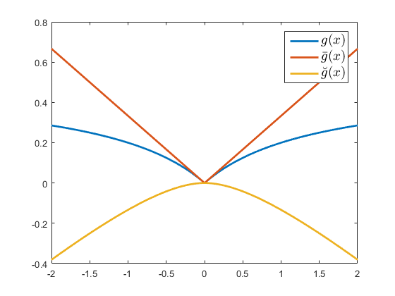
(a) GP.

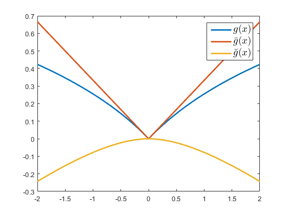
(b) LSP.

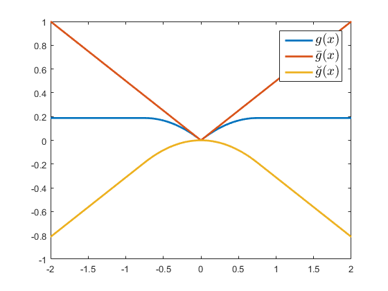
(c) MCP.

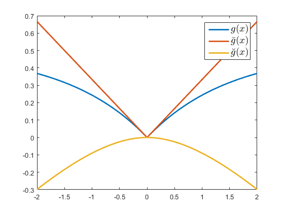
(d) Laplace.

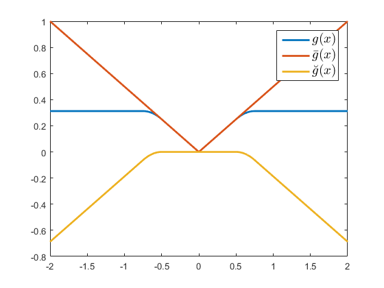
(e) SCAD.

Figure 1: Decompositions of the regularizers in Table 1 for one-dimensional $z$ ($\beta=0.5$, $\theta=1.5$).

Using Corollary 3, problem (1) can then be rewritten as

$$\min_{x}\bar{f}(x)+\breve{g}(x),$$ (20)

where $\bar{f}(x)\equiv f(x)+\bar{g}(x)$. Note that $\bar{f}$ (which can be viewed as an augmented loss) is Lipschitz smooth while $\breve{g}$ (viewed as a convexified regularizer) is convex but possibly nonsmooth. In other words, nonconvexity is shifted from the regularizer $g$ to the loss $f$, while ensuring that the augmented loss is smooth.

When $X$ is a matrix, similar to Corollary 3, the following Proposition 5 holds for $g$ in C2.

Proposition 5

Any $g$ in C2 can be decomposed as $\bar{g}(X)+\breve{g}(X)$, where

$$\bar{g}(X)\equiv\mu\sum_{i=1}^{m}\kappa(\sigma_{i}(X))-\mu\kappa_{0}\|X\|_{*}$$ (21)

is concave and $2\rho$-Lipschitz smooth, while $\breve{g}(X)\equiv\kappa_{0}\|X\|_{*}$ is convex and nonsmooth.

Since $\bar{g}$ is concave and $\breve{g}$ is convex, the nonconvex regularizer $g=\breve{g}-(-\bar{g})$ can be viewed as a difference of convex functions (DC) (Hiriart-Urruty, 1985). Lu (2012); Gong et al. (2013); Zhong and Kwok (2014) also relied on DC decompositions of the nonconvex regularizer. However, they do not utilize this in the computational procedures, while we use the DC decomposition to simplify the regularizers. As will be seen, though the DC decomposition of a nonconvex function is not unique in general, the particular one proposed here is crucial for efficient optimization.

4 Example Use Cases

In this section, we provide concrete examples to show how the proposed convexification scheme can be used with various optimization algorithms. An overview is summarized in Table 2.

Table 2: Using the proposed convexification scheme with various algorithms.

	section	advantages
proximal algorithm	4.1, 4.6	cheaper proximal step
FW algorithm	4.2	cheaper linear subproblem
(consensus) ADMM	4.3	cheaper proximal step; provide convergence guarantee
SVRG	4.4	cheaper proximal step; provide convergence guarantee
mOWL-QN	4.5	simpler analysis; capture curvature information

4.1 Proximal Algorithms

In this section, we provide example applications on using the proximal algorithm for nonconvex structured sparse learning. The proximal algorithm has been commonly used for learning with convex regularizers (Parikh and Boyd, 2013). With a nonconvex regularizer, the underlying proximal step becomes much more challenging. Gong et al. (2013); Li and Lin (2015) and Bot et al. (2016) extended proximal algorithm to simple nonconvex $g$, but cannot handle more complicated nonconvex regularizers such as the tree-structured lasso regularizer (Liu and Ye, 2010; Schmidt et al., 2011), sparse group lasso regularizer (Jacob et al., 2009) and total variation regularizer (Nikolova, 2004). Using the proximal average (Bauschke et al., 2008), Zhong and Kwok (2014) can handle nonconvex regularizers of the form $g=\sum_{i=1}^{K}\mu_{i}g_{i}$, where each $g_{i}$ is simple. However, the solutions obtained are only approximate. General nonconvex optimization techniques such as the concave-convex procedure (CCCP) (Yuille and Rangarajan, 2002) or its variant sequential convex programming (SCP) (Lu, 2012) can also be used, though they are slow in general (Gong et al., 2013; Zhong and Kwok, 2014).

Using the proposed transformation, one only needs to solve the proximal step of a standard convex regularizer instead of that of a nonconvex regularizer. This allows reuse of existing solutions for the proximal step and is much less expensive. As proximal algorithms have the same convergence guarantee for convex and nonconvex $f$ (Gong et al., 2013; Li and Lin, 2015), solving the transformed problem can be much faster. The following gives some specific examples.

4.1.1 Nonconvex Sparse Group Lasso

In sparse group lasso, the feature vector $x$ is divided into groups. Assume that group $\mathcal{G}_{j}$ contains dimensions in $x$ that group $j$ contains. Let $\left[x_{\mathcal{G}_{j}}\right]_{i}=x_{i}$ if $i\in\mathcal{G}_{j}$, and 0 otherwise. Given training samples $\{(a_{1},y_{1}),\dots,(a_{N},y_{N})\}$, (convex) sparse group lasso is formulated as (Jacob et al., 2009):

$$\min_{x}\sum_{i=1}^{N}\ell(y_{i},a_{i}^{\top}x)+\lambda\|x\|_{1}+\sum_{j=1}^{K}\mu_{j}\|x_{\mathcal{G}_{j}}\|_{2},$$ (22)

where $\ell$ is a smooth loss, and $K$ is the number of (non-overlapping) groups.

For the nonconvex extension, the regularizer becomes

$$g(x)=\lambda\sum_{i=1}^{d}\kappa(|x_{i}|)+\sum_{j=1}^{K}\mu_{j}\kappa(\|x_{\mathcal{G}_{j}}\|_{2}).$$ (23)

Using Corollary 3 and Remark 4, the convexified regularizer is $\breve{g}(x)=\kappa_{0}(\lambda\|x\|_{1}+\sum_{j=1}^{K}\mu_{j}\|x_{\mathcal{G}_{j}}\|_{2})$. Its proximal step can be easily computed by the algorithm in (Yuan et al., 2011). Specifically, the proximal operator of $\breve{g}$ can be obtained by computing $\text{prox}_{\mu_{j}\|\cdot\|_{2}}(\text{prox}_{\lambda\|\cdot\|_{1}}(x_{\mathcal{G}_{j}}))$ for each group separately. This can then be used with any proximal algorithm that can handle nonconvex objectives (as $\bar{f}$ is nonconvex). In particular, we will adopt the state-of-the-art nonmontonic APG (nmAPG) algorithm (Li and Lin, 2015) (shown in Algorithm 2). Note that nmAPG cannot be directly used with the nonconvex regularizer $g$ in (23), as the corresponding proximal step has no inexpensive closed-form solution.

Algorithm 2 Nonmonotonic APG (nmAPG) (Li and Lin, 2015).

1:  Initialize $z_{1}=x_{1}=x_{0}$, $\alpha_{0}=0$, $\alpha_{1}=1$, $\eta\in[0,1)$, $c_{1}=F(x_{1})$, $q_{1}=1$, and stepsize $\tau>\bar{L}$, $\delta\in(0,\tau-\bar{L})$;

2:  for $t=1,\dots,T$ do

3:     $y_{t}=x_{t}+\frac{\alpha_{t-1}}{\alpha_{t}}(z_{t}-x_{t})+\frac{\alpha_{t-1}-1}{\alpha_{t}}(x_{t}-x_{t-1})$;

4:     $z_{t+1}=\text{prox}_{\frac{1}{\tau}\breve{g}}(y_{t}-\frac{1}{\tau}\nabla\bar{f}(y_{t}))$;

5:     if $F(z_{t+1})\leq c_{t}-\frac{\delta}{2}\|z_{t+1}-y_{t}\|_{2}^{2}$ then

6:        $x_{t+1}=z_{t+1}$;

7:     else

8:        $v_{t+1}=\text{prox}_{\frac{1}{\tau}\breve{g}}(x_{t}-\frac{1}{\tau}\nabla\bar{f}(x_{t}))$;

9:        $x_{t+1}=\begin{cases}z_{t+1}&F(z_{t+1})\leq F(v_{t+1})\\ v_{t+1}&\text{otherwise}\end{cases}$;

10:     end if

11:     $\alpha_{t+1}=\frac{1}{2}(\sqrt{4\alpha_{t}^{2}+1}+1)$;

12:     $q_{t+1}=\eta q_{t}+1$;

13:     $c_{t+1}=\frac{\eta q_{t}c_{t}+F(x_{t+1})}{q_{t+1}}$;

14:  end for

15:  return  $x_{T+1}$;

As mentioned in Section 3, the proposed decomposition of the nonconvex regularizer $g$ can be regarded as a DC decomposition, which is not unique in general. For example, we might try to add a quadratic term to convexify the nonconvex regularizer. Specifically, we can decompose $g(x)$ in (23) as $\tilde{\varsigma}(x)+\hat{\varsigma}(x)$, where

$$\tilde{\varsigma}(x)=\lambda\sum_{i=1}^{d}\left(\kappa(|x_{i}|)+\frac{\rho}{2}x_{i}^{2}\right)+\sum_{j=1}^{K}\mu_{j}\left(\kappa(\|x_{\mathcal{G}_{j}}\|_{2})+\frac{\rho}{2}\|x_{\mathcal{G}_{j}}\|_{2}^{2}\right),$$ (24)

and $\hat{\varsigma}(x)=-\frac{\rho}{2}\sum_{j=1}^{K}(\mu_{j}+\lambda)\|x_{\mathcal{G}_{j}}\|_{2}^{2}$. It can be easily shown that $\hat{\varsigma}$ is concave, and Proposition 6 shows that $\tilde{\varsigma}$ is convex. Thus, $F$ can be transformed as $F(x)=\bar{f}(x)+\tilde{\varsigma}(x)$, where $\bar{f}(x)=f(x)+\hat{\varsigma}(x)$ is Lipschitz-smooth, and $\tilde{\varsigma}$ is convex but nonsmooth. However, the proximal step associated with $\tilde{\varsigma}$ has no simple closed-form solution.

Proposition 6

$\kappa(\|\cdot\|_{2})+\frac{\rho}{2}\|\cdot\|_{2}^{2}$ is convex.

4.1.2 Nonconvex Tree-Structured Group Lasso

In (convex) tree-structured group lasso (Liu and Ye, 2010; Jenatton et al., 2011), the dimensions in $x$ are organized as nodes in a tree, and each group corresponds to a subtree. The regularizer is of the form $\sum_{j=1}^{K}\lambda_{j}\|x_{\mathcal{G}_{j}}\|_{2}$. Interested readers are referred to (Liu and Ye, 2010) for details.

For the nonconvex extension, $g(x)$ becomes $\sum_{j=1}^{K}\lambda_{j}\kappa(\|x_{\mathcal{G}_{j}}\|_{2})$. Again, there is no closed-form solution of its proximal step. On the other hand, the convexified regularizer is $\breve{g}(x)\equiv\kappa_{0}\sum_{j=1}^{K}\lambda_{j}\|x_{\mathcal{G}_{j}}\|_{2}$. As shown in (Liu and Ye, 2010), its proximal step can be computed efficiently by processing all the groups once in some appropriate order.

4.1.3 Nonconvex Total Variation (TV) Regularizer

In an image, nearby pixels are usually strongly correlated. The TV regularizer captures such behavior by assuming that changes between nearby pixels are small. Given an image $X\in\mathbb{R}^{m\times n}$, the TV regularizer is defined as $\text{TV}(X)=\|D_{v}X\|_{1}+\|XD_{h}\|_{1}$ (Nikolova, 2004), $D_{v}=\begin{bmatrix}-1&1&&\\ &\ddots&\ddots&\\ &&-1&1\end{bmatrix}\in\mathbb{R}^{(m-1)\times m}$ and $D_{h}=\begin{bmatrix}-1&&\\ 1&\ddots&\\ &\ddots&-1\\ &&1\end{bmatrix}\in\mathbb{R}^{n\times(n-1)}$ are the horizontal and vertical partial derivative operators, respectively. Thus, it is popular on image processing problems, such as image denoising and deconvolution (Nikolova, 2004; Beck and Teboulle, 2009).

As in previous sections, the nonconvex extension of TV regularizer can be defined as

$$\sum_{i=1}^{m-1}\sum_{j=1}^{m}\kappa\left(\left|\left[D_{v}X\right]_{ij}\right|\right)+\sum_{i=1}^{n}\sum_{j=1}^{n-1}\kappa\left(\left|\left[XD_{h}\right]_{ij}\right|\right).$$ (25)

Again, it is not clear how its proximal step can be efficiently computed. However, with the proposed transformation, the transformed problem is

$$\min_{X}\bar{f}(X)+\mu\kappa_{0}\text{TV}(X),$$

where $\mu$ is the regularization parameter, $\bar{f}(X)=f(X)+\mu\sum_{i=1}^{m-1}\sum_{j=1}^{m}(\kappa(|[D_{v}X]_{ij}|)-\kappa_{0}|[D_{v}X]_{ij}|)+\mu\sum_{i=1}^{n}\sum_{j=1}^{n-1}(\kappa(|[XD_{h}]_{ij}|)-\kappa_{0}|[XD_{h}]_{ij}|)$ is concave and Lipschitz smooth. One then only needs to compute the proximal step of the standard TV regularizer.

However, unlike the proximal steps in Sections 4.1.1 and 4.1.2, the proximal step of the TV regularizer has no closed-form solution and needs to be solved iteratively. In this case, Schmidt et al. (2011) showed that using inexact proximal steps can make proximal algorithms faster. However, they only considered the situation where both $f$ and $g$ are convex. In the following, we extend nmAPG (Algorithm 2), which can be used with nonconvex objectives, to allow for inexact proximal steps (steps 5 and 9 of Algorithm 3). However, Lemma 2 of (Li and Lin, 2015), which is key to the convergence of nmAPG, no longer holds dues to inexact proximal step. To fix this problem, in step 6 of Algorithm 3, we use $F(X_{t})$ instead of $c_{t}$ in Algorithm 2. Besides, we also drop the comparison of $F(Z_{t+1})$ and $F(V_{t+1})$ (originally in step 9 of Algorithm 2).

Algorithm 3 Inexact nmAPG.

1:  Initialize $\tilde{Z}_{1}=X_{1}=X_{0}$, $\alpha_{0}=0$, $\alpha_{1}=1$ and stepsize $\tau>\bar{L}$, $\delta\in(0,\tau-\bar{L})$;

2:  for $t=1,\dots,T$ do

3:     choose tolerance $\epsilon_{t}$;

4:     $Y_{t}=X_{t}+\frac{\alpha_{t-1}}{\alpha_{t}}(Z_{t}-X_{t})+\frac{\alpha_{t-1}-1}{\alpha_{t}}(X_{t}-X_{t-1})$;

5:     $\tilde{Z}_{t+1}$ = approximate $\text{prox}_{\frac{1}{\tau}\breve{g}}(Y_{t}-\frac{1}{\tau}\nabla\bar{f}(Y_{t}))$, with inexactness $\vartheta_{t+1}\leq\epsilon_{t}$;

6:     if $F(\tilde{Z}_{t+1})\leq F(X_{t})-\frac{\delta}{2}\|\tilde{Z}_{t+1}-Y_{t}\|_{F}^{2}$ then

7:        $X_{t+1}=\tilde{Z}_{t+1}$;

8:     else

9:        $X_{t+1}$ = approximate $\text{prox}_{\frac{1}{\tau}\breve{g}}(X_{t}-\frac{1}{\tau}\nabla\bar{f}(X_{t}))$, with inexactness $\vartheta_{t+1}\leq\epsilon_{t}$;

10:     end if

11:     $\alpha_{t+1}=\frac{1}{2}(\sqrt{4\alpha_{t}^{2}+1}+1)$;

12:  end for

13:  return  $X_{T+1}$;

Inexactness of the proximal step can be controlled as follows. Let $P=X-\frac{1}{\tau}\nabla\bar{f}(X)$, and $h(X)\equiv\frac{1}{2}\|X-P\|_{F}^{2}+\frac{1}{\tau}\breve{g}(X)$ be the objective in $\text{prox}_{\frac{1}{\tau}\breve{g}}(P)$. As $\breve{g}(X)=\kappa_{0}\text{TV}(X)$ is convex, $h$ is also convex. Let $\tilde{X}$ be an inexact solution of this proximal step. The inexactness $h(\tilde{X})-h(\text{prox}_{\frac{1}{\tau}\breve{g}}(P))$ is upper-bounded by the duality gap $\vartheta\equiv h(\tilde{X})-\mathcal{D}(\tilde{W})$, where $\mathcal{D}$ is the dual of $h$, and $\tilde{W}$ is the corresponding dual variable. In step 5 (resp. step 9) of Algorithm 3, we solve the proximal step until its duality gap $\vartheta_{t+1}$ is smaller than a given threshold $\epsilon_{t}$. The following Theorem shows convergence of Algorithm 3.

Theorem 7

Let $\sum_{t=1}^{\infty}\epsilon_{t}<\infty$. The sequence $\{X_{t}\}$ generated from Algorithm 3 has at least one limit point, and every limit point is also a critical point of (1).

If the proximal step is exact, $\|V_{t}-\text{prox}_{\frac{1}{\tau}\breve{g}}(V_{t}-\frac{1}{\tau}\nabla\bar{f}(V_{t}))\|_{F}^{2}$ can be used to measure how far $V_{t}$ is from a critical point (Gong et al., 2013; Ghadimi and Lan, 2016). In Algorithm 3, the proximal step is inexact, and $X_{t+1}$ is an inexact solution to $\text{prox}_{\frac{1}{\tau}\breve{g}}(V_{t}-\frac{1}{\tau}\nabla\bar{f}(V_{t}))$, where $V_{t}=Y_{t}$ if step 7 is executed, and $V_{t}=X_{t}$ if step 9 is executed. As $X_{t+1}$ converges to a critical point of (1), we propose using $d_{t}\equiv\|X_{t+1}-V_{t}\|_{F}^{2}$ to measure how far $X_{t+1}$ is from a critical point. The following Proposition shows a $O(1/T)$ convergence rate on $\min_{t=1,\dots,T}d_{t}$.

Proposition 8

(i) $\lim_{t\rightarrow\infty}d_{t}=0$; and (ii) $\min_{t=1,\dots,T}d_{t}$ converges to zero at a rate of $O(1/T)$.

Note that the (exact) nmAPG in Algorithm 2 cannot handle the nonconvex $g$ in (25) efficiently, as the corresponding proximal step has no closed-form solutions but has to be solved exactly. Even the proposed inexact nmAPG (Algorithm 3) cannot be directly used with nonconvex $g$. As the dual of the nonconvex proximal step is difficult to derive and the optimal duality gap is nonzero in general, the proximal step’s inexactness cannot be easily controlled.

4.2 Frank-Wolfe Algorithm

In this section, we use the Frank-Wolfe algorithm to learn a low-rank matrix $X\in\mathbb{R}^{m\times n}$ for matrix completion as reviewed in Section 2.3. The nuclear norm regularizer in (8) may over-penalize top singular values. Recently, there is growing interest to replace this with nonconvex regularizers (Lu et al., 2014, 2015; Yao et al., 2015; Gui et al., 2016). Hence, instead of (8), we consider

$$\min_{X}f(X)+\mu\sum_{i=1}^{m}\kappa(\sigma_{i}(X)).$$ (26)

When $\kappa$ is the identity function, (26) reduces to (8). Note that the FW algorithm cannot be directly used on (8), as its linear subproblem in (10) then becomes $\min_{S:\sum_{i=1}^{m}\kappa(\sigma_{i}(S))\leq 1}\langle S,\nabla f(X_{t})\rangle$, which is difficult to osolve.

Using Proposition 5, problem (26) is transformed into

$$\min_{X}\bar{f}(X)+\bar{\mu}\|X\|_{*},$$ (27)

where

$$\bar{f}(X)=f(X)+\bar{g}(X),\;\;\bar{g}(X)=\mu\sum_{i=1}^{m}(\kappa(\sigma_{i}(X))-\kappa_{0}\sigma_{i}(X)),$$ (28)

and $\bar{\mu}=\mu\kappa_{0}$. This only involves the standard nuclear norm regularizer. However, Algorithm 1 still cannot be used as $\bar{f}$ in (28) is no longer convex. A FW variant allowing nonconvex $\bar{f}$ is proposed in (Bredies et al., 2009). However, condition 1 in (Bredies et al., 2009) requires $g$ to satisfy $\lim_{\|X\|_{F}\rightarrow\infty}\frac{g(X)}{\|X\|_{F}}=\infty$. Such condition does not hold with $g(X)=\|X\|_{*}$ in (27) as

$$\frac{\|X\|_{*}}{\|X\|_{F}}=\sqrt{\frac{(\sum_{i=1}^{m}\sigma_{i})^{2}}{\sum_{i=1}^{m}\sigma_{i}^{2}}}\leq\sqrt{\frac{m\sum_{i=1}^{m}\sigma_{i}^{2}}{\sum_{i=1}^{m}\sigma_{i}^{2}}}=\sqrt{m}<\infty.$$

In the following, we propose a nonconvex FW variant (Algorithm 4) for the transformed problem (27). It is similar to Algorithm 1, but with three important modifications. First, $\bar{g}(X)$ in (28) depends on the singular values of $X$, which cannot be directly obtained from the $UV^{\top}$ factorization in (11). Instead, we use the low-rank factorization

$$X=UBV^{\top},$$ (29)

where $U\in\mathbb{R}^{m\times k}$, $V\in\mathbb{R}^{n\times k}$ are orthogonal and $B\in\mathcal{S}_{+}^{k\times k}$ is positive semidefinite.

Algorithm 4 Frank-Wolfe algorithm for solving the nonconvex problem (27).

1:  $U_{1}=[\;]$, $B_{1}=[\;]$ and $V_{1}=[\;]$;

2:  for $t=1\dots T$ do

3:     $[u_{t},s_{t},v_{t}]=\text{rank1SVD}(\nabla\bar{f}(X_{t}))$;

4:     obtain $\alpha_{t}$ and $\beta_{t}$ from (32);

5:     $[\bar{U}_{t},\bar{B}_{t},\bar{V}_{t}]=\text{warmstart}(U_{t},u_{t},V_{t},v_{t},B_{t},\alpha_{t},\beta_{t})$;

6:     obtain $[U_{t+1},B_{t+1},V_{t+1}]$ from (33), using $\bar{U}_{t}$, $\bar{B}_{t}$ and $\bar{V}_{t}$ for warm-start; // $X_{t+1}=U_{t+1}B_{t+1}V_{t+1}^{\top}$

7:  end for

8:  return  $U_{T+1}$, $B_{T+1}$ and $V_{T+1}$.

The second problem is that line search in Algorithm 1 is inefficient in general when operated on a nonconvex $\bar{f}$. Specifically, step 4 in Algorithm 1 then becomes

$$[\alpha_{t},\beta_{t}]=\arg\min_{\alpha\geq 0,\beta\geq 0}\bar{f}(\alpha X_{t}+\beta u_{t}v_{t}^{\top})+\bar{\mu}(\alpha\|X_{t}\|_{*}+\beta).$$ (30)

To solve (30), we have to compute $\frac{\partial\bar{f}(S)}{\partial\alpha}$ and $\frac{\partial\bar{f}(S)}{\partial\beta}$, where $S=\alpha X_{t}+\beta u_{t}v_{t}^{\top}$. As shown in Proposition 9, this requires the SVD of $S$ and can be expensive.

Proposition 9

Let the SVD of $S$ be $U_{S}\text{Diag}([\sigma_{1}(S),\dots,\sigma_{m}(S)])V_{S}^{\top}$. Then

$$\frac{\partial\bar{f}(S)}{\partial\alpha}=\alpha\langle X_{t},\nabla\bar{f}(S)\rangle,\quad\text{and}\quad\frac{\partial\bar{f}(S)}{\partial\beta}=\beta u_{t}^{\top}\nabla\bar{f}(S)v_{t},$$

where $\nabla\bar{f}(S)=\nabla f(S)+\mu U_{S}\text{Diag}(w)V_{S}^{\top}$, and $w=[\kappa^{\prime}(\sigma_{i}(S))-\kappa_{0}]\in\mathbb{R}^{m}$.

Corollary 10

For $X$ in (29), let the SVD of $B$ be $U_{B}\text{Diag}([\sigma_{1}(B),\dots,\sigma_{k}(B)])V_{B}^{\top}$. Then, $\nabla\bar{f}(X)=\nabla f(X)+\bar{\mu}(UU_{B})\text{Diag}(w)(VV_{B})^{\top}$, where $w=[\kappa^{\prime}(\sigma_{i}(B))-\kappa_{0}]\in\mathbb{R}^{k}$.

Alternatively, as $S$ is a rank one updates of $X_{t}$, one can perform incremental update on SVD, which takes $O((m+n)t^{2})$ time (Golub and Van Loan, 2012). However, every time $\alpha,\beta$ are changed, this incremental SVD has to be recomputed, and is thus inefficient.

To alleviate this problem, we approximate $\bar{f}(S)$ by the upper bound as

$$\bar{f}(S) = \bar{f}(X_{t}+(\alpha-1)X_{t}+\beta u_{t}v_{t}^{\top})$$ (31)

$$\leq \bar{f}(X_{t})+\langle(\alpha-1)X_{t}+\beta u_{t}v_{t}^{\top},\nabla\bar{f}(X_{t})\rangle+\frac{\bar{L}}{2}\|(\alpha-1)X_{t}+\beta u_{t}v_{t}^{\top}\|_{F}^{2}.$$

As $(u_{t},v_{t})$ is obtained from the rank-$1$ SVD of $\nabla\bar{f}(X_{t})$, we have $\|u_{t}v_{t}^{\top}\|_{F}=1$ and $u_{t}^{\top}\nabla\bar{f}(X_{t})v_{t}=s_{t}$. Moreover, $X_{t}=U_{t}B_{t}V_{t}^{\top}$, and so $\|X_{t}\|_{F}=\|B_{t}\|_{F}$ and $\|X_{t}\|_{*}=\text{\,Tr}\left(B_{t}\right)$. Substituting these and the upper bound (31) into (30), we obtain a simple quadratic program:

$$\min_{\alpha\geq 0,\beta\geq 0} \frac{(\alpha-1)^{2}\bar{L}}{2}\|B_{t}\|_{F}^{2}+(\alpha-1)\beta\bar{L}(u_{t}^{\top}U_{t})B_{t}(V_{t}^{\top}v_{t})+\frac{\beta^{2}\bar{L}}{2}+\beta s_{t}$$ (32)

$$+\alpha\langle B_{t},U_{t}^{\top}\nabla\bar{f}(X_{t})V_{t}\rangle+\bar{\mu}(\alpha\|B_{t}\|_{*}+\beta).$$

Note that the objective in (32) is convex, as the RHS in (31) is convex and the last term from (30) is affine. Moreover, using Corollary 10, $\langle B_{t},U_{t}^{\top}\nabla\bar{f}(X_{t})V_{t}\rangle$ in (32) can be obtained as

$$\langle B_{t},U_{t}^{\top}\nabla\bar{f}(X_{t})V_{t}\rangle=\langle B_{t},U_{t}^{\top}\nabla f(X_{t})V_{t}\rangle+\bar{\mu}\sum_{i=1}^{t}\sigma_{i}(B_{t})(\kappa^{\prime}(\sigma_{i}(B_{t}))-\kappa_{0}).$$

Instead of requiring SVD on $X_{t}$, it only requires SVD on $B_{t}$ (which is of size $t\times t$ at the $t$th iteration of Algorithm 4). As the target matrix is supposed to be low-rank, $t\ll m$. Hence, all the coefficients in (32) can be obtained in $O((m+n)t^{2}+\|\Omega\|_{1}t)$ time. Besides, (32) is a quadratic program with only two variables, and thus can be very efficiently solved.

The third modification is that with $\bar{f}$ instead of $f$, (12) can no longer be used for local optimization, as $\bar{g}(X)$ in (28) depends on the singular values of $X$. On the other hand, with the decomposition of $X$ in (29) and Proposition 11 below, (27) can be rewritten as

$$\min_{U,B,V} f(UBV^{\top})+\bar{g}(B)+\bar{\mu}\text{\,Tr}\left(B\right)$$ (33)

s.t. $$U^{\top}U=I,V^{\top}V=I,B\in\mathcal{S}_{+}.$$ (34)

This can be efficiently solved using matrix optimization techniques on the Grassmann manifold (Ngo and Saad, 2012).

Proposition 11

For orthogonal matrices $U$ and $V$, $\bar{g}(UBV^{\top})=\bar{g}(B)$.

In Algorithm 4, step 5 is used to warm-start (33), and the procedure is shown in Algorithm 5. It expresses $X_{t}=\alpha_{t}U_{t-1}B_{t-1}V_{t-1}^{\top}+\beta_{t}u_{t}v_{t}^{\top}$ obtained in step 4 to the form $U_{t}B_{t}V_{t}^{\top}$ so that the orthogonal constraints on $U_{t},V_{t}$ in (34) are satisfied.

Algorithm 5 $\text{warmstart}(U_{t},u_{t},V_{t},v_{t},B_{t},\alpha_{t},\beta_{t})$.

1:  $[\bar{U}_{t},R_{\bar{U}_{t}}]=\text{QR}([U_{t},u_{t}])$; // QR denotes the QR factorization

2:  $[\bar{V}_{t}\,,R_{\bar{V}_{t}}]=\text{QR}([V_{t},\,v_{t}])$;

3:  $\bar{B}_{t}=R_{\bar{U}_{t}}\begin{bmatrix}\alpha_{t}B_{t}&0\\ 0&\beta_{t}\end{bmatrix}R_{\bar{V}_{t}}^{\top}$;

4:  return  $\bar{U}_{t}$, $\bar{B}_{t}$ and $\bar{V}_{t}$;

Existing analysis for the FW algorithm cannot be used on this nonconvex problem. The following Theorem shows convergence of Algorithm 4 to a critical point of (8).

Theorem 12

If (8) has a rank-$r$ critical point, then Algorithm 4 converges to a critical point of (8) after $r$ iterations.

4.3 Alternating Direction Method of Multipliers (ADMM)

In this section, we consider using ADMM on the consensus optimization problem (16). When all the $f_{i}$’s and $g$ are convex, ADMM has a convergence rate of $O(1/T)$ (He and Yuan, 2012). Recently, ADMM has been extended to problems where $g$ is convex but $f_{i}$’s are nonconvex (Hong et al., 2016). However, when $g$ is nonconvex, such as when a nonconvex regularizer is used in regularized risk minimization, the convergence of ADMM is still an open reseach problem.

Using the proposed transformation, we can decompose a nonconvex $g$ as $\bar{g}+\breve{g}$, where $\bar{g}$ is concave and Lipschitz-smooth, while $\breve{g}$ is convex but possibly nonsmooth. Problem (16) can then be rewritten as

$$\min_{y,x^{1},\dots,x^{M}}\sum_{i=1}^{M}\bar{f}_{i}(x^{i})+\breve{g}(y)\;\;:\;\;x^{1}=\dots=x^{M}=y,$$ (35)

where $\bar{f}_{i}(x)=f_{i}(x)+\frac{1}{M}\bar{g}(x)$. Let $p^{i}$ be the dual variable for the constraint $x^{i}=y$. The augmented Lagrangian for (35) is

$$\mathcal{L}\left(y,x^{1},\dots,x^{M},p^{1},\dots,p^{M}\right)=\breve{g}(y)+\sum_{i=1}^{M}\bar{f}_{i}(x^{i})+(p^{i})^{\top}(x^{i}-y)+\frac{\tau}{2}\|x^{i}-y\|_{2}^{2}.$$ (36)

Using (14) and (15), we have the following update equations at iteration $t$:

$$x^{i}_{t+1} = \arg\min_{x^{i}}\bar{f}_{i}(x^{i})+(p^{i}_{t})^{\top}(x^{i}-y_{t})+\frac{\tau}{2}\|x^{i}-y_{t}\|_{2}^{2},$$

$$y_{t+1} = \arg\min_{y}\frac{1}{2}\left\|y-\sum_{i=1}^{M}\left(x^{i}_{t}+\frac{1}{\tau}p^{i}_{t}\right)\right\|_{2}^{2}+\frac{1}{\tau}\breve{g}(y)=\text{prox}_{\frac{1}{\tau}\breve{g}}\left(\sum_{i=1}^{M}x^{i}_{t}+\frac{1}{\tau}p^{i}_{t}\right).$$ (37)

As in previous sections, the proximal step in (37), which is associated with the convex $\breve{g}$, is usually easier to compute than the proximal step associated with the original nonconvex $g$. Moreover, since $\breve{g}$ is convex, convergence results in Theorem 2.4 of (Hong et al., 2016) can now be applied. Specifically, the sequence $\{y_{t},\{x^{i}_{t}\}\}$ generated by the ADMM procedure converges to a critical point of (35).

4.4 Stochastic Variance Reduced Gradient

Variance reduction methods have been commonly used to speed up the often slow convergence of stochastic gradient descent (SGD). Examples are stochastic variance reduced gradient (SVRG) (Johnson and Zhang, 2013) and its proximal extension Prox-SVRG (Xiao and Zhang, 2014). They can be used for the following optimization problem

$$\min_{x}\sum_{i=1}^{N}\ell(y_{i},a_{i}^{\top}x)+g(x),$$ (38)

where $\{(a_{1},y_{1}),\dots,(a_{N},y_{N})\}$ are the training samples, $\ell$ is a smooth convex loss function, and $g$ is a convex regularizer. Recently, Prox-SVRG is also extended for nonconvex objectives. Reddi et al. (2016a) and Zhu and Hazan (2016) considered smooth nonconvex $\ell$ but without $g$. This is further extended to the case of smooth $\ell$ and convex nonsmooth $g$ in (Reddi et al., 2016b). However, convergence is still unknown for the more general case where the regularizer $g$ is also nonconvex.

Using the proposed transformation, (38) can be rewritten as

$$\min_{x}\sum_{i=1}^{N}\left(\ell(y_{i},a_{i}^{\top}x)+\frac{1}{N}\bar{g}(x)\right)+\breve{g}(x),$$

where $\ell+\frac{1}{N}\bar{g}$ is smooth and $\breve{g}$ is convex. As a result, convergence results in (Reddi et al., 2016b) can now be applied.

4.5 With OWL-QN

In this section, we consider OWL-QN (Andrew and Gao, 2007) and its variant mOWL-QN (Gong and Ye, 2015b), which are efficient algorithms for the $\ell_{1}$-regularization problem

$$\min_{x}f(x)+\mu\|x\|_{1}.$$ (39)

Recently, Gong and Ye (2015a) proposed a nonconvex generalization for (39), in which the standard $\ell_{1}$ regularizer is replaced by the nonconvex $g(x)=\mu\sum_{i=1}^{d}\kappa(|x_{i}|)$:

$$\min_{x}f(x)+\mu\sum_{i=1}^{d}\kappa(|x_{i}|).$$ (40)

Gong and Ye (2015a) proposed a sophisticated algorithm (HONOR) which involves a combination of quasi-Newton and gradient descent steps. Though the algorithm is similar to OWL-QN and mOWL-QN, the convergence analysis in (Gong and Ye, 2015b) cannot be directly applied as the regularizer is nonconvex. Instead, a non-trivial extension was developed in (Gong and Ye, 2015a).

Here, by convexifying the nonconvex regularizer, (40) can be rewritten as

$$\min_{x}\bar{f}(x)+\mu\kappa_{0}\|x\|_{1},$$ (41)

where $\bar{f}(x)=f(x)+\bar{g}(x)$, and $\bar{g}(x)=\mu\sum_{i=1}^{d}(\kappa(|x_{i}|)-\kappa_{0}|x_{i}|)$. It is easy to see that the analysis in (Gong and Ye, 2015b) can be extended to handle smooth but nonconvex $\bar{f}$. Thus, mOWL-QN is still guaranteed to converge to a critical point.

As demonstrated in previous sections, other DC decompositions of $g$ are not as useful. For example, with the one in Proposition 6, we obtain the convex regularizer $\breve{\varsigma}(x)=\frac{\rho\mu}{2}\|x\|_{2}^{2}+\mu\sum_{i=1}^{d}\kappa(|x_{i}|)$. However, mOWL-QN can no longer be applied, as it works only with the $\ell_{1}$-regularizer.

Problem (40) can be solved by either (i) directly using HONOR, or (ii) using mOWL-QN on the transformed problem (41). We believe that the latter approach is computationally more efficient. In (40), the Hessian depends on both terms in the objective, as the second-order derivative of $\kappa$ is not zero in general. However, HONOR constructs the approximate Hessian using only information from $f$, and thus ignores the curvature information due to $\sum_{i=1}^{d}\kappa(|x_{i}|)$. On the other hand, the Hessian in (41) depends only on $\bar{f}$, as the Hessian due to $\|x\|_{1}$ is zero (Andrew and Gao, 2007), and mOWL-QN now extracts Hessian from $\bar{f}$. Hence, optimizing (41) with mOWL-QN is potentially faster, as all the second-order information is utilized. This will be verified empirically in Section 5.4.

4.6 Nonsmooth and Nonconvex Loss

In many applications, besides having nonconvex regularizers, the loss function may also be nonconvex and nonsmooth. Thus, neither $f$ nor $g$ in (1) is convex, smooth. The optimization problem becomes even harder, and many existing algorithms cannot be used. In particular, the proximal algorithm requires $f$ in (1) to be smooth (possibly nonconvex) (Gong et al., 2013; Li and Lin, 2015; Bot et al., 2016). The FW algorithm requires $f$ in (4) to be smooth and convex (Jaggi, 2013). For the ADMM, it allows $f$ in the consensus problem to be smooth, but $g$ has to be convex (Hong et al., 2016). For problems of the form $\min_{x,z}f(y)+g(y):y=Ax$, ADMM requires $A$ to have full row-rank (Li and Pong, 2015). As will be seen, it is not satisfied for problems considered in this section. CCCP (Yuille and Rangarajan, 2002) and smoothing (Chen, 2012) are more general and can still be used, but are usually very slow.

In this section, we consider two application examples, and show how they can be efficiently solved with the proposed transformation.

4.6.1 Total Variation Image Denoising

Using the $\ell_{1}$ loss and TV regularizer introduced in Section 4.1.3, consider the following optimization problem:

$$\min_{X}\|Y-X\|_{1}+\mu\text{TV}(X),$$ (42)

where $Y\in\mathbb{R}^{m\times n}$ is a given corrupted image, and $X$ is the target image to be recovered. The use of nonconvex loss and regularizer often produce better performance (Yan, 2013). Thus, we consider the following nonconvex extension:

$$\min_{X}\sum_{i=1}^{m}\sum_{j=1}^{n}\kappa\left(\left|\left[Y-X\right]_{ij}\right|\right)+\mu\sum_{i=1}^{m-1}\sum_{j=1}^{m}\kappa\left(\left|\left[D_{v}X\right]_{ij}\right|\right)+\mu\sum_{i=1}^{n}\sum_{j=1}^{n-1}\kappa\left(\left|\left[XD_{h}\right]_{ij}\right|\right),$$ (43)

where both the loss and regularizer are nonconvex and nonsmooth. As discussed above, this can be solved by CCCP and smoothing. However, as will be experimentally demonstrated in Section 5.5, their convergence is slow.

Using the proposed transformation on both the loss and regularizer, problem (43) can be transformed to the following problem:

$$\min_{X}\bar{f}(X)+\kappa_{0}\|X-Y\|_{1}+\kappa_{0}\mu\text{TV}(X),$$ (44)

where

$$\bar{f}(X)= \sum_{i=1}^{m}\sum_{j=1}^{n}\kappa\left(\left|\left[Y-X\right]_{ij}\right|\right)-\kappa_{0}\|Y-X\|_{1}$$

$$+\mu\left[\sum_{i=1}^{m-1}\sum_{j=1}^{m}\kappa\left(\left|\left[D_{v}X\right]_{ij}\right|\right)-\kappa_{0}\|D_{v}X\|_{1}+\sum_{i=1}^{n}\sum_{j=1}^{n-1}\kappa\left(\left|\left[XD_{h}\right]_{ij}\right|\right)-\kappa_{0}\|XD_{h}\|_{1}\right]$$

is smooth and nonconvex. As (44) is not a consensus problem, the method in (Hong et al., 2016) cannot be used. To use the ADMM algorithm in (Li and Pong, 2015), extra variables and constraints $Z_{v}=D_{v}X$ and $Z_{h}=XD_{h}$ have to be imposed. However, the full row-rank condition in (Li and Pong, 2015) does not hold.

In this section, we consider the proximal algorithm. Given some $Z$, the proximal step in (44) is

$$\arg\min_{X}\frac{1}{2}\|X-Z\|_{F}^{2}+\frac{1}{\tau}\left(\|X-Y\|_{1}+\mu\text{TV}(X)\right),$$ (45)

where $\tau$ is the stepsize. Though this has no closed-form solution, $\|X-Y\|_{1}+\mu\text{TV}(X)$ in (45) is convex and one can thus monitor inexactness of the proximal step via the duality gap. Thus, we can use the proposed inexact nmAPG algorithm in Algorithm 3 for (44). It can be shown that the dual of (45) is

$$\min_{W,P,Q} \frac{1}{2\tau}\|W+\mu D_{v}^{\top}P+\mu QD_{h}^{\top}\|_{F}^{2}-\langle Z,W\rangle-\mu\langle D_{v}Z,P\rangle-\mu\langle ZD_{h},Q\rangle+\langle Y,W\rangle$$ (46)

 s.t. $$\|W\|_{\infty}\leq 1,\|P\|_{\infty}\leq 1\;\text{and}\;\|Q\|_{\infty}\leq 1,$$

and the primal variable can be recovered as $X=Z-\frac{1}{\tau}(W+\mu D_{v}^{\top}P+\mu QD_{h}^{\top})$. By substituting the obtained $X$ into (45) and $\{W,P,Q\}$ into (46), the duality gap can be computed in $O(mn)$ time. As (46) is a smooth and convex problem, both accelerated gradient descent (Nesterov, 2013) and L-BFGS (Nocedal and Wright, 2006) can be applied. Algorithm 3 is then guaranteed to converge to a critical point of (43) (Theorem 7 and Proposition 8).

Note that it is more advantageous to transform both the loss and regularizer in (44). If only the regularizer in (43) is transformed, we obtain

$$\bar{f}_{\text{TV}}(X)+\sum_{i=1}^{m}\sum_{j=1}^{n}\kappa\left(\left|\left[Y-X\right]_{ij}\right|\right)+\kappa_{0}\mu\text{TV}(X),$$ (47)

where

$$\bar{f}_{\text{TV}}(X)=\mu\left[\sum_{i=1}^{m-1}\sum_{j=1}^{m}\kappa\left(\left|\left[D_{v}X\right]_{ij}\right|\right)-\kappa_{0}\|D_{v}X\|_{1}+\sum_{i=1}^{n}\sum_{j=1}^{n-1}\kappa\left(\left|\left[XD_{h}\right]_{ij}\right|\right)-\kappa_{0}\|XD_{h}\|_{1}\right]$$

is nonconvex. The corresponding proximal step for (47) is

$$\arg\min_{X}\frac{1}{2}\|X-Z\|_{F}^{2}+\frac{1}{\tau}\left(\sum_{i=1}^{m}\sum_{j=1}^{n}\kappa\left(\left|\left[Y-X\right]_{ij}\right|\right)+\kappa_{0}\mu\text{TV}(X)\right).$$ (48)

While the proximal steps in both (45) and (48) have no closed-form solution, working with (45) is more efficient. As (45) is convex, its dual can be efficiently solved with methods such as accelerated gradient descent and L-BFGS. In contrast, (48) is nonconvex, its duality gap is nonzero, and so can only be solved in the primal with slower methods like CCCP and smoothing. Besides, one can only use the more expensive nmAPG (Algorithm 2) but not the proposed inexact proximal algorithm.

4.6.2 Robust Sparse Coding

The second application is robust sparse coding, which has been popularly used in face recognition (Yang et al., 2011), image analysis (Lu et al., 2013) and background modeling (Zhao et al., 2011). Given an observed signal $y\in\mathbb{R}^{m}$, the goal is to seek a robust sparse representation $x\in\mathbb{R}^{d}$ of $y$ based on the dictionary $D\in\mathbb{R}^{m\times d}$ (which is assumed to be fixed here). Mathematically, it is formulated as the following optimization problem:

$$\min_{x}\|y-Dx\|_{1}+\mu\|x\|_{1}.$$

Its nonconvex extension is:

$$\min_{x}\sum_{j=1}^{m}\kappa(|[y-Dx]_{j}|)+\mu\sum_{i=1}^{d}\kappa(|x_{i}|).$$ (49)

Using the proposed transformation, problem (49) becomes

$$\min_{x}\bar{f}(x)+\kappa_{0}\|y-Dx\|_{1}+\mu\kappa_{0}\|x\|_{1},$$ (50)

where

$$\bar{f}(x)=\mu\sum_{j=1}^{d}\kappa(|x_{j}|)-\kappa_{0}\mu\|x\|_{1}+\sum_{j=1}^{m}\kappa(|[y-Dx]_{j}|)-\kappa_{0}\|y-Dx\|_{1}$$

is smooth and nonconvex. Again, we use the inexact nmAPG algorithm in Algorithm 3. The proximal step for (50) is

$$\arg\min_{x}\frac{1}{2}\|x-z\|_{2}^{2}+\frac{1}{\tau}(\|y-Dx\|_{1}+\mu\|x\|_{1}),$$ (51)

where $\tau$ is the stepsize and $z$ is given. As in Section 4.6.1, $\|y-Dx\|_{1}+\mu\|x\|_{1}$ in (51) is convex, and one can monitor inexactness of the proximal step by the duality gap. The dual of (51) is

$$\min_{p,q}\frac{1}{2\tau}\|D^{\top}p+\mu q\|_{2}^{2}-p^{\top}Dz-\mu q^{\top}z\;:\;\|p\|_{\infty}\leq 1,\|q\|_{\infty}\leq 1.$$ (52)

As in (46), this can be solved with L-BFGS or accelerated gradient descent. The primal variable can be recovered as $x=z-\frac{1}{\tau}(D^{\top}p+\mu q)$, and the duality gap can be checked in $O(md)$ time.

If only the regularizer is transformed, we obtain

$$\min_{x}\sum_{j=1}^{m}\kappa(|[y-Dx]_{j}|)+\bar{f}_{\text{RSC}}(x)+\kappa_{0}\mu\|x\|_{1},$$ (53)

where $\bar{f}_{\text{RSC}}(x)=\mu\sum_{j=1}^{d}\kappa(|x_{j}|)-\kappa_{0}\mu\|x\|_{1}$. The corresponding proximal step is

$$\arg\min_{x}\frac{1}{2}\|x-z\|_{2}^{2}+\sum_{j=1}^{m}\kappa(|[y-Dx]_{j}|)+\kappa_{0}\mu\|x\|_{1},$$ (54)

which still involve the nonconvex function $\kappa$. As in Section 4.6.1, (52) is easier to solve than (54).

5 Experiments

In this section, we perform experiments on using the proposed procedure with (i) proximal algorithms (Sections 5.1 and 5.2); (ii) Frank-Wolfe algorithm (Section 5.3); (iii) comparision with HONOR (Section 5.4) and (vi) image denoising (Section 5.5). Experiments are performed on a PC with Intel i7 CPU and 32GB memory. All algorithms are implemented in Matlab.

5.1 Nonconvex Sparse Group Lasso

In this section, we perform experiments on the nonconvex sparse group lasso model in Section 4.1.1. For simplicity, assume that $\mu_{1}=\dots=\mu_{K}=\mu$. Using the square loss, (22) becomes

$$\min_{x}\frac{1}{2}\|y-A^{\top}x\|_{2}^{2}\!+\!\lambda\sum_{i=1}^{d}\kappa(|x_{i}|)\!+\!\mu\sum_{j=1}^{K}\kappa(\|x_{\mathcal{G}_{j}}\|_{2}),$$ (55)

where $A=[a_{1},\dots,a_{N}]$. In this experiment, we use the LSP regularizer in Table 1 (with $\theta=0.5$) as $\kappa(\cdot)$. The synthetic data set is generated as follows. Let $d=10000$. The ground-truth parameter $\bar{x}\in\mathbb{R}^{10000}$ is divided into $100$ non-overlapping groups: $\{1,\dots,100\}$, $\{101,\dots,200\}$, $\dots$, $\{9901,\dots,10000\}$ (Figure 2). We randomly set $75\%$ of the groups to zero. In each nonzero group, we randomly set $25\%$ of its features to zero, and generate the nonzero features from the standard normal distribution $\mathcal{N}(0,1)$. The whole data set has $20,000$ samples, and entries of the input matrix $A\in\mathbb{R}^{10000\times 20000}$ are generated from $\mathcal{N}(0,1)$. The ground-truth output is $\bar{y}=A^{\top}\bar{x}$. This is then corrupted by random Gaussian noise $\epsilon$ in $\mathcal{N}(0,0.05)$ to produce $y=\bar{y}+\epsilon$.

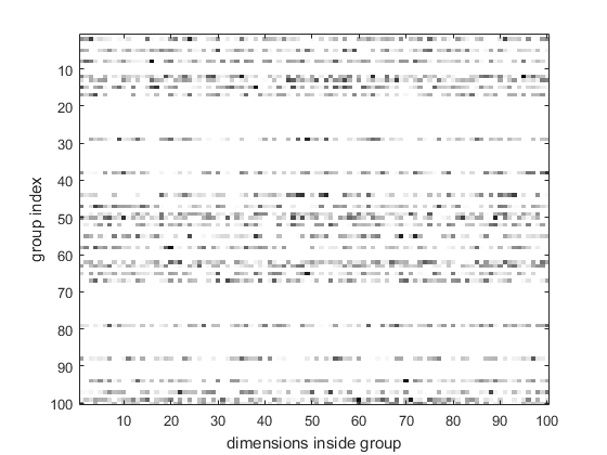
Figure 2: An example ground-truth parameter $\bar{x}\in\mathbb{R}^{10000}$. It is reshaped as a $100\times 100$ matrix, with each row representing a group.

The proposed algorithm will be called N2C (Nonconvex-to-Convex). The proximal step of the convexified regularizer $\breve{g}(x)=\kappa_{0}(\lambda\|x\|_{1}+\sum_{j=1}^{K}\mu_{j}\|x_{\mathcal{G}_{j}}\|_{2})$ is obtained using the algorithm in (Yuan et al., 2011). The nmAPG algorithm (Algorithm 2) in (Li and Lin, 2015) is used for optimization. This will be compared with the following state-of-the-art algorithms:

1. SCP: Sequential convex programming (Lu, 2012), in which the LSP regularizer is decomposed following (24).

2. GIST (Gong et al., 2013): Since the nonconvex regularizer is not separable, the associated proximal operator has no closed-form solution. Instead, we use SCP (with warm-start) to solve it numerically.

3. GD-PAN (Zhong and Kwok, 2014): It performs gradient descent with proximal average (Bauschke et al., 2008) of the nonconvex regularizers. Closed-form solutions for the proximal operator of each regularizer are obtained separately, and then averaged.

4. nmAPG with the original nonconvex regularizer: As in GIST, the proximal step is solved numerically by SCP.

5. As a baseline, we also compare with the FISTA (Beck, 2009) algorithm, which solves the convex sparse group lasso model (with $\kappa$ removed from (55)).

We do not compare with the concave-convex procedure (Yuille and Rangarajan, 2002), which has been shown to be slow (Gong et al., 2013; Zhong and Kwok, 2014).

We use $50\%$ of the data for training, another $25\%$ as validation set to tune $\lambda,\mu$ in (55), and the rest for testing. The stepsize is fixed at $\tau=\sigma_{1}(A^{\top}A)$. For performance evaluation, we use the (i) testing root-mean-squared error (RMSE) on the predictions; (ii) absolute error between the obtained parameter $\hat{x}$ with ground-truth $\bar{x}$: $\text{ABS}=\|\hat{x}-\bar{x}\|_{1}/d$; and (iii) CPU time. To reduce statistical variability, the experimental results are averaged over 5 repetitions.

Results are shown in Table 3. As can be seen, all the nonconvex models obtain better errors (RMSE and ABS) than the convex FISTA. As for the training speed, N2C is the fastest. SCP, GIST, nmAPG and N2C targets the original problem (1), and they have the same recovery performance. GD-PAN solves an approximate problem in each of its iterations, and its error is slightly worse than the other nonconvex algorithms on this data set.

Table 3: Results on nonconvex sparse group lasso. RMSE and ABS are scaled by $10^{-3}$, and the CPU time is in seconds. The best and comparable results (according to the pairwise t-test with 95% confidence) are highlighted.

	non-accelerated			accelerated		convex
	SCP	GIST	GD-PAN	nmAPG	N2C	FISTA
RMSE	50.6$\pm$2.0	50.6$\pm$2.0	52.3$\pm$2.0	50.6$\pm$2.0	50.6$\pm$2.0	53.8$\pm$1.7
ABS	5.7$\pm$0.2	5.7$\pm$0.2	7.1$\pm$0.4	5.7$\pm$0.2	5.7$\pm$0.2	10.6$\pm$0.3
CPU time(sec)	0.84$\pm$0.14	0.92$\pm$0.12	0.94$\pm$0.22	0.65$\pm$0.06	0.48$\pm$0.05	0.79$\pm$0.14

Figure 3 shows convergence of the objective with time and iterations for a typical run. SCP, GIST, nmAPG and N2C all converge towards the same objective value. GD-PAN can only approximate the original problem. Thus, it converges to an objective value which is larger than others. nmAPG and N2C are based on the state-of-the-art proximal algorithm (Algorithm 2. Both require nearly the same number of iterations for convergence (Figure 3(a)). However, as N2C has cheap closed-form solution for its proximal step, it is much faster when measured in terms of time (Figure 3(b)). Overall, N2C, which uses acceleration and inexpensive proximal step, is the fastest.

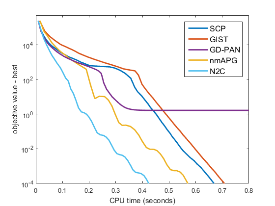
(a) objective vs CPU time.

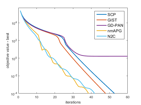
(b) objective vs iterations.

Figure 3: Convergence of algorithms on nonconvex sparse group lasso. FISTA is not shown as its (convex) objective is different from the others.

5.2 Nonconvex Tree-Structured Group Lasso

In this section, we perform experiments on the nonconvex tree-structured group lasso model in Section 4.1.2. We use the face data set JAFFE, which contains $213$ images with seven facial expressions: anger, disgust, fear, happy, neutral, sadness and surprise. Following (Liu and Ye, 2010), we resize each image from $256\times 256$ to $64\times 64$. Their tree structure, which is based on pixel neighborhoods, is also used here. The total number of groups $K$ is $85$.

Since our goal is only to demonstrate usefulness of the proposed convexification scheme, we focus on the binary classification problem “anger vs not-anger” (with 30 anger images and 183 non-anger images). The logistic loss is used, which is more appropriate for classification. Given training samples $\{(a_{1},y_{1}),\dots,(a_{N},y_{N})\}$, the optimization problem is then

$$\min_{x}\sum_{i=1}^{N}\!w_{i}\log(1+\exp(-y_{i}\cdot a_{i}^{\top}x))+\mu\sum_{i=1}^{K}\lambda_{i}\kappa(\|x_{\mathcal{G}_{i}}\|_{2}),$$

where $\kappa(\cdot)$ is the LSP regularizer (with $\theta=0.5$),, $w_{i}$’s are weights (set to be the reciprocal of the size of sample $i$’s class) used to alleviate class imbalance, and $\lambda_{i}=1/\sqrt{\|\mathcal{G}_{i}\|_{1}}$ as in (Liu and Ye, 2010). We use $60\%$ of the data for training, $20\%$ for validation and the rest for testing. For the proposed N2C algorithm, the proximal step of the convexified regularizer is obtained as in (Liu and Ye, 2010).

As in Section 5.1, it is compared with SCP, GIST, GD-PAN, nmAPG, and FISTA. The stepsize $\eta$ is obtained by line search. For performance evaluation, we use (i) the testing accuracy; (ii) solution sparsity (i.e., percentage of nonzero elements); and (iii) CPU time. To reduce statistical variability, the experimental results are averaged over 5 repetitions.

Results are shown in Table 4. As can be seen, all nonconvex models have similar testing accuracies, and they again outperform the convex model. Moreover, solutions from the nonconvex models are sparser. Overall, N2C is the fastest and has the sparsest solution.

Table 4: Results on tree-structured group lasso. The best and comparable results (according to the pairwise t-test with 95% confidence) are highlighted.

	non-accelerated			accelerated		convex
	SCP	GIST	GD-PAN	nmAPG	N2C	FISTA
testing accuracy (%)	99.6$\pm$0.9	99.6$\pm$0.9	99.6$\pm$0.9	99.6$\pm$0.9	99.6$\pm$0.9	97.2$\pm$1.8
sparsity (%)	5.5$\pm$0.4	5.7$\pm$0.4	6.9$\pm$0.4	5.4$\pm$0.3	5.1$\pm$0.2	9.2$\pm$0.2
CPU time(sec)	7.1$\pm$1.6	50.0$\pm$8.1	14.2$\pm$2.6	3.8$\pm$0.4	1.9$\pm$0.3	1.0$\pm$0.4

Figure 4 shows convergence of the algorithms versus CPU time and number of iterations. As can be seen, N2C is the fastest. GIST is the slowest, as it does not utilize acceleration and its proximal step is solved numerically which is expensive. GD-PAN converges to a less optimal solution due to its use of approximation. Moreover, as in Section 5.1, nmAPG and N2C show similar convergence behavior w.r.t. the number of iterations (Figure 4(b)), but N2C is much faster w.r.t. time (Figure 4(a)).

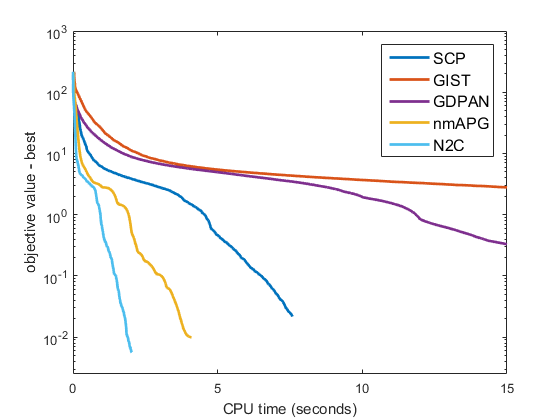
(a) objective vs CPU time (seconds).

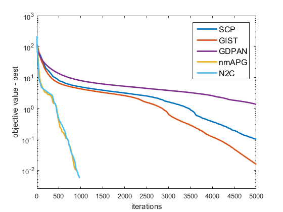
(b) the objective vs iterations.

Figure 4: Convergence of algorithms on nonconvex tree-structured group lasso.

5.3 Nonconvex Low-Rank Matrix Completion

In this section, we perform experiments on nonconvex low-rank matrix completion (Section 4.2), with square loss in (26). The LSP regularizer is used, with $\theta=\sqrt{\mu}$ as in (Yao et al., 2015). We use the MovieLens data sets (Table 5), which have been commonly used for evaluating matrix completion (Hsieh and Olsen, 2014; Yao et al., 2015). They contain ratings $\{1,2,\dots,5\}$ assigned by various users on movies.

Table 5: MovieLens data sets used in the experiment.

	#users	#items	#ratings
100K	943	1,682	100,000
1M	6,040	3,449	999,714
10M	69,878	10,677	10,000,054

The proposed Frank-Wolfe procedure (Algorithm 4), denoted N2C-FW, is compared with the following algorithms:

1. FaNCL (Yao et al., 2015): This is a recent nonconvex matrix regularization algorithm. It is based on the proximal algorithm using efficient approximate SVD and automatic thresholding of singular values.

2. LMaFit (Wen et al., 2012): It factorizes $X$ as a product of low-rank matrices $U\in\mathbb{R}^{m\times k}$ and $V\in\mathbb{R}^{n\times k}$. The nonconvex objective $\frac{1}{2}\|P_{\Omega}(UV^{\top}-O)\|_{F}^{2}$ is then minimized by alternating minimization on $U$ and $V$ using gradient descent.

3. Active subspace selection (denoted “active”) (Hsieh and Olsen, 2014): This solves the (convex) nuclear norm regularized problem (with $\kappa$ being the identity function in (8)) by using the active row/column subspaces to reduce the optimization problem size.

We do not compare with IRNN (Lu et al., 2014) and GPG (Lu et al., 2015), which have been shown to be much slower than FaNCL (Yao et al., 2015).

Following (Yao et al., 2015), we use $50\%$ of the ratings for training, $25\%$ for validation and the rest for testing. For performance evaluation, we use (i) the testing RMSE; and (ii) the recovered rank. To reduce statistical variability, the experimental results are averaged over 5 repetitions.

Results are shown in Table 6. As can be seen, the nonconvex models (N2C-FW, FaNCL and LMaFit) achieve lower RMSEs than the convex model (active), with N2C-FW having the smallest RMSE. Moreover, the convex model needs a much higher rank than the nonconvex models, which agrees with the previous observations in (Mazumder et al., 2010; Yao et al., 2015). Thus, its running time is also much longer than the others. Figure 5 shows the convergence of the objective with CPU time. As the recovered matrixs rank for the nonconvex models are very low (2 to 9 in Table 6), N2C-FW is much faster than the others as it starts from a rank-one matrix and only increases its rank by one in each iteration. Though FaNCL uses singular value thresholding to truncate the SVD, it does not control the rank as directly as N2C-FW and so is still slower.

Table 6: Results on the MovieLens data sets. The best RMSE’s (according to the pairwise t-test with 95% confidence) are highlighted.

		RMSE	rank	CPU time(sec)
100K	N2C-FW	0.855$\pm$0.004	2	0.2$\pm$0.1
	FaNCL	0.857$\pm$0.003	2	0.4$\pm$0.1
	LMaFit	0.867$\pm$0.004	2	0.3$\pm$0.1
	(convex) active	0.875$\pm$0.002	52	1.8$\pm$0.1
1M	N2C-FW	0.785$\pm$0.001	5	9.3$\pm$0.1
	FaNCL	0.786$\pm$0.001	5	16.6$\pm$0.6
	LMaFit	0.812$\pm$0.002	5	14.7$\pm$0.7
	(convex) active	0.811$\pm$0.001	106	46.3$\pm$1.1
10M	N2C-FW	0.778$\pm$0.001	9	313.0$\pm$6.6
	FaNCL	0.779$\pm$0.001	9	615.7$\pm$13.2
	LMaFit	0.797$\pm$0.001	9	491.9$\pm$36.3
	(convex) active	0.808$\pm$0.001	137	1049.8$\pm$43.2

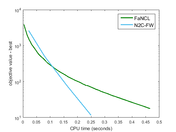
(a) MovieLens-100K.

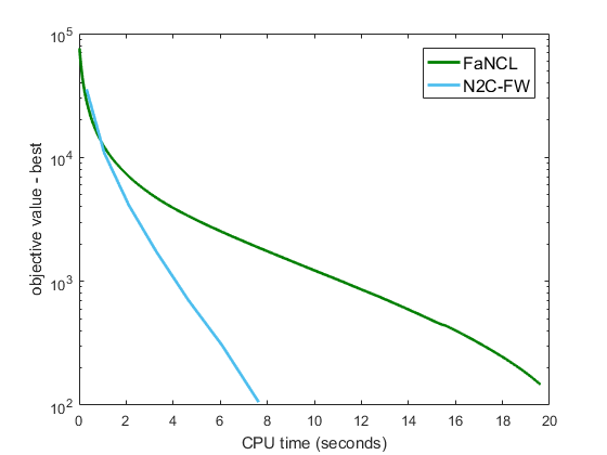
(b) MovieLens-1M.

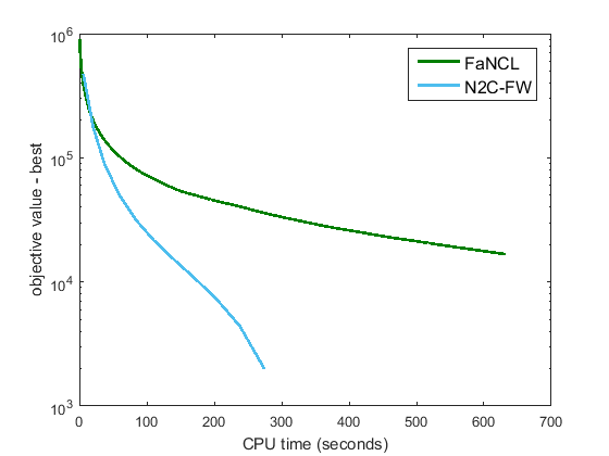
(c) MovieLens-10M.

Figure 5: Convergence of the objective vs CPU time on nonconvex low-rank matrix completion. The objectives of LMaFit and active subspace selection are different from N2C-FW, and thus are not shown.

5.4 Comparison with HONOR

In this section, we experimentally compare the proposed method with HONOR (Section 4.5) on the model in (40), using the logistic loss and LSP regularizer. Following (Gong and Ye, 2015a), we fix $\mu=1$ in (40), and $\theta$ in the LSP regularizer to $0.01\mu$. Experiments are performed on three large data sets, kdd2010a, kdd2010b and url (Table 7). Both kdd2010a and kdd2010b are educational data sets, and the task is to predict students’ successful attempts to answer concepts related to algebra. The url data set contains a collection of websites, and the task is to predict whether a particular website is malicious. We compare

1. running HONOR (Gong and Ye, 2015a) directly on (40). The threshold of the hybrid step in HONOR is set to $10^{-10}$, which yields the best empirical performance in (Gong and Ye, 2015a);

2. running mOWL-QN (Gong and Ye, 2015b)) on the transformed problem (41).

To reduce statistical variability, the experimental results are averaged over 5 repetitions.

Table 7: Data sets used in the comparison with HONOR.

	kdd2010a	kdd2010b	url
number of samples	510,302	748,401	2,396,130
number of features	20,216,830	29,890,095	3,231,961

As (40) and (41) have the same optimization objective, Figure 6 shows the convergence of the objective with CPU time. As can be seen, mOWL-QN converges faster than HONOR. This validates our claim that the curvature information of the nonconvex regularizer helps.

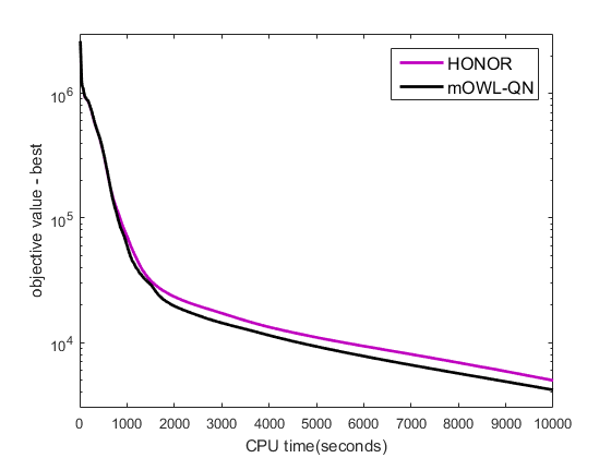
(a) kdd2010a.

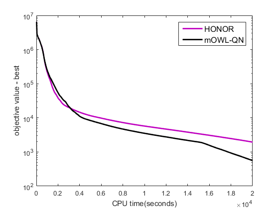
(b) kdd2010b.

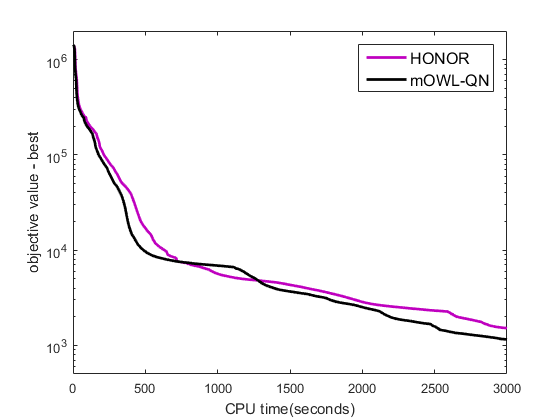
(c) url.

Figure 6: Convergence of the objective vs CPU time for HONOR and mOWL-QN.

5.5 Image Denoising

In this section, we perform experiments on total variation image denoising with nonconvex loss and nonconvex regularizer (as introduced in Section 4.6.1). The LSP function (with $\theta=1$) is used as $\kappa$ in (43) on both the loss and regularizer. Eight popular images from (Dabov et al., 2007) are used (Figure 7). They are then corrupted by pepper-and-salt noise, with $10\%$ of the pixels randomly set to $0$ or $255$ with equal probabilities.

For performance evaluation, we use the $\text{RMSE}=\sqrt{\frac{1}{mn}\sum_{i=1}^{m}\sum_{j=1}^{n}(X_{ij}-\bar{X}_{ij})^{2}}$, where $\bar{X}\in\mathbb{R}^{m\times n}$ is the clean image, and $X\in\mathbb{R}^{m\times n}$ is the recovered image. To tune $\mu$, we pick the value that leads to the smallest RMSE on the first four images (boat, couple, fprint, hill). Denoising performance is then reported on the remaining images (house, lena, man, peppers).

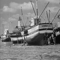
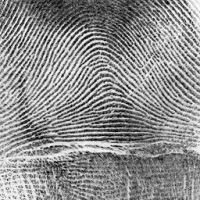
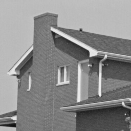
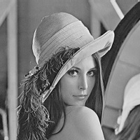
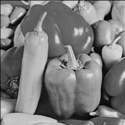
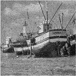
(a) boat.

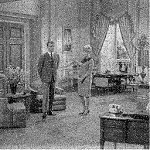
(b) couple.

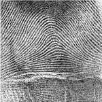
(c) fprint.

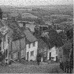
(d) hill.

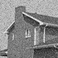
(e) house.

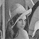
(f) lena.

(g) man.

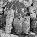
(h) peppers.

Figure 7: Samples images used in the denoising experiment. Top: Clean images; Bottom: Noisy images.

The following algorithms will be compared:

1. CCCP (Yuille and Rangarajan, 2002): Proposition 6 is used to construct DC decomposition for $\kappa$ (Details are at Appendix B.1);

2. Smoothing (Chen, 2012): The nonsmooth $\kappa$ is smoothed, and then gradient descent is used (Details are at Appendix B.2);

3. nmAPG (Li and Lin, 2015): This optimizes (47) with Algorithm 2, and the exact proximal step is solved numerically using CCCP;

4. inexact-nmAPG: This optimizes (44) with Algorithm 3 (with $\epsilon_{t}=0.95^{t}$), and the inexact proximal step is solved numerically using L-BFGS.

5. As a baseline, we also compare with ADMM (Boyd et al., 2011) with the convex formulation.

To reduce statistical variability, the experimental results are averaged over 5 repetitions. The RMSE results are shown in Table 8. As can be seen, the (convex) ADMM formulation leads to the highest RMSE, while CCCP, smoothing, nmAPG and inexact-nmAPG have the same RMSE which is lower than that of ADMM. This agrees with previous observations that nonconvex formulations can yield better performance than the convex ones. Timing results are shown in Table 9 and Figure 8. As can be seen, smoothing has low iteration complexity but suffers from slow convergence. CCCP and nmAPG both need to exactly solve a subproblem, and thus are also slow. The inexact-nmAPG algorithm does not guarantee the objective value to be monotonically decreasing as iteration proceeds. As the inexactness is initially large, there is an initial spike in the objective. However, inexact-nmAPG then quickly converges, and is much faster than all the baselines.

Table 8: RMSE for image denoising. The best RMSE’s (according to the pairwise t-test with 95% confidence) are highlighted.

	house	lena	man	peppers
CCCP	0.0205$\pm$0.0010	0.0174$\pm$0.0005	0.0223$\pm$0.0002	0.0207$\pm$0.0009
smoothing	0.0205$\pm$0.0011	0.0174$\pm$0.0005	0.0223$\pm$0.0002	0.0207$\pm$0.0009
nmAPG	0.0205$\pm$0.0010	0.0174$\pm$0.0005	0.0223$\pm$0.0002	0.0207$\pm$0.0009
inexact-nmAPG	0.0205$\pm$0.0010	0.0174$\pm$0.0005	0.0223$\pm$0.0002	0.0207$\pm$0.0009
(convex) ADMM	0.0223$\pm$0.0011	0.0193$\pm$0.0005	0.0242$\pm$0.0002	0.0229$\pm$0.0008

Table 9: CPU time (seconds) for image denoising. The shortest CPU time (according to the pairwise t-test with 95% confidence) are highlighted.

	house	lena	man	peppers
CCCP	21.0$\pm$2.3	270.0$\pm$13.0	325.3$\pm$17.4	14.5$\pm$1.2
smoothing	75.5$\pm$2.0	433.1$\pm$4.8	437.7$\pm$6.8	61.9$\pm$1.7
nmAPG	19.4$\pm$2.3	91.4$\pm$7.3	104.4$\pm$2.7	16.1$\pm$1.8
inexact-nmAPG	10.3$\pm$1.1	37.9$\pm$5.0	43.0$\pm$7.6	8.1$\pm$0.2
(convex) ADMM	3.0$\pm$0.1	42.8$\pm$1.1	46.9$\pm$1.0	2.2$\pm$0.1

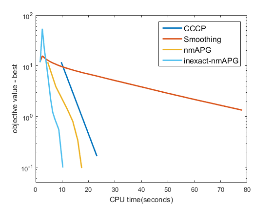
(a) house.

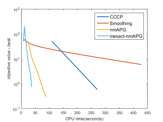
(b) lena.

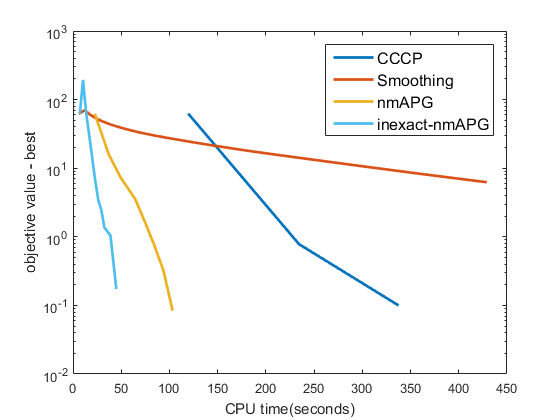
(c) man.

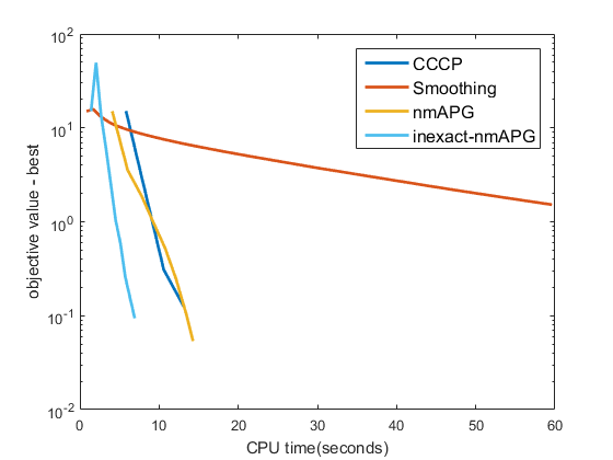
(d) peppers.

Figure 8: CPU time (seconds) vs objective value on different images.

6 Conclusion

In this paper, we proposed a novel approach to learning with nonconvex regularizers. By moving the nonconvexity associated with the nonconvex regularizer to the loss, the nonconvex regularizer is convexified to become a familiar convex regularizer while the augmented loss is still Lipschitz smooth. This allows one to reuse efficient algorithms originally designed for convex regularizers on the transformed problem. To illustrate usages with the proposed transformation, we plug it into many popular optimization algorithms. First, we consider the proximal algorithm, and showed that while the proximal step is expensive on the original problem, it becomes much easier on the transformed problem. We further propose an inexact proximal algorithm, which allows inexact update of proximal step when it does not have a closed-form solution. Second, we combine the proposed convexification scheme with the Frank-Wolfe algorithm on learning low-rank matrices, and showed that its crucial linear programming step becomes cheaper and more easily solvable. As no convergence results exist on this nonconvex problem, we designed a novel Frank-Wolfe algorithm based on the proposed transformation and with convergence guarantee. Third, when using with ADMM and SVRG, we showed that the existing convergence results can be applied on the transformed problem but not on the original one. We further extend the proposed transformation to handle nonconvex and nonsmooth loss functions, and illustrate its benefits on the total variation model and robust sparse coding. Finally, we demonstrate the empirical advantages of working with the transformed problems on various tasks with both synthetic and real-world data sets. Experimental results show that better performance can be obtained with nonconvex regularizers, and algorithms on the transformed problems run much faster than the state-of-the-art on the original problems.

A Proofs

A.1 Proposition 1

Proof  First, we introduce a few Lemmas.

Lemma 13

(Golub and Van Loan, 2012) For $x\neq 0$, the gradient of the $\ell_{2}$-norm is $\nabla_{x_{i}}\|x\|_{2}=x_{i}/\|x\|_{2}$.

Let $h(z)=\kappa(\|z\|_{2})-\kappa_{0}\|z\|_{2}$.

Lemma 14

$$\nabla_{z_{i}}h(z)=\left\{\begin{array}[]{ll}\frac{\kappa^{\prime}(\|z\|_{2})-\kappa_{0}}{\|z\|_{2}}z_{i}&\text{if}\;z\neq 0\\ 0&\text{otherwise}\end{array}\right..$$ (56)

Proof  For $z\neq 0$, $\|z\|_{2}$ is differentiable (Lemma 13), and we obtain the first part of (56). For $z=0$, let $\bar{h}_{i}(z)=\frac{\kappa^{\prime}(\|z\|_{2})-\kappa_{0}}{\|z\|_{2}}z_{i}$. Consider any $\Delta$ with $\|\Delta\|_{2}=1$.

$$\lim_{\alpha\rightarrow 0^{+}}{\bar{h}_{i}(0+\alpha\Delta)} =\lim_{\alpha\rightarrow 0^{+}}\frac{\kappa^{\prime}(\|\alpha\Delta\|_{2})-\kappa_{0}}{\|\alpha\Delta\|_{2}}\alpha\Delta_{i},$$

$$=\lim_{\alpha\rightarrow 0^{+}}(\kappa^{\prime}(\alpha)-\kappa_{0})\Delta_{i}=0,$$

as $\lim_{\alpha\rightarrow 0^{+}}\kappa^{\prime}(\alpha)-\kappa_{0}=0$. Thus, $h(z)$ is smooth at $z=0$, and we obtain the second part of (56).  

Lemma 15

(Eriksson et al., 2004) Let $f:\mathbb{R}\rightarrow\mathbb{R}$ be a differentiable function. (i) If its derivative $f^{\prime}$ is bounded, then $f$ is Lipschitz-continuous with constant equal to the maximum value of $|f^{\prime}|$.

Lemma 16

(Eriksson et al., 2004) If a continuous function $f:\mathbb{R}\rightarrow\mathbb{R}$ is $L_{1}$-Lipschitz continuous in $[a,b]$ and $L_{2}$-Lipschitz continuous in $[b,c]$ (where $-\infty\leq a<b<c\leq\infty$), then it is $\max(L_{1},L_{2})$-Lipschitz continuous in $[a,c]$.

Lemma 17

Let $z$ be an arbitrary vector, and $e_{i}$ be the unit vector with only its $i$th dimension equal to $1$. Define $\hat{h}_{i}(\gamma)=\frac{\kappa^{\prime}(\|z+e_{i}\gamma\|_{2})-\kappa_{0}}{\|z+e_{i}\gamma\|_{2}}(z_{i}+\gamma)$. Then, $\hat{h}$ is $2\rho$-Lipschitz continuous.

Proof  Since $\kappa^{\prime}$ is non-differentiable only at finite points, and let them be $\{\hat{\alpha}_{1},\dots,\hat{\alpha}_{k}\}$ where $\hat{\alpha}_{1}<\dots<\hat{\alpha}_{k}$. We partition $(-\infty,\infty)$ into intervals $(-\infty,\hat{\alpha}_{1}]\cup[\hat{\alpha}_{1},\hat{\alpha}_{2}]\cup\cdots\cup[\hat{\alpha}_{k},\infty)$, such that $\kappa^{\prime\prime}$ exists in each interval. Let $w=z+e_{i}\gamma$. For any interval,

$$\hat{h}_{i}^{\prime}(\gamma)=\frac{\kappa^{\prime\prime}(\|w\|_{2})}{\|w\|_{2}}(z_{i}+\gamma)^{2}+\left(1-\frac{(z_{i}+\gamma)^{2}}{\|w\|_{2}^{2}}\right)\frac{\kappa^{\prime}(\|w\|_{2})-\kappa_{0}}{\|w\|_{2}}.$$ (57)

Let $\phi(\alpha)=\kappa^{\prime}(\alpha)-\kappa_{0}$, where $\alpha\geq 0$. Note that $\phi(0)=0$. Moreover, $\phi(\alpha)$ is $\rho$-Lipschitz continuous as $\kappa$ is $\rho$-Lipschitz smooth. Thus,

$$|\phi(\alpha)-\phi(0)|=|\kappa^{\prime}(\alpha)-\kappa_{0}|\leq\rho\alpha,$$

and so

$$\left|\kappa^{\prime}(\|w\|_{2})-\kappa_{0}\right|\leq\rho\|w\|_{2}.$$ (58)

Note that $(z_{i}+\gamma)^{2}\leq\|w\|_{2}^{2}$, (57) can be written as

$$\left|\hat{h}_{i}^{\prime}(\gamma)\right| \leq\left|\frac{\kappa^{\prime\prime}(\|w\|_{2})}{\|w\|_{2}}(z_{i}+\gamma)^{2}\right|+\left|\left(1-\frac{(z_{i}+\gamma)^{2}}{\|w\|_{2}^{2}}\right)\frac{\kappa^{\prime}(\|w\|_{2})-\kappa_{0}}{\|w\|_{2}}\right|$$

$$\leq\left|\kappa^{\prime\prime}(\|w\|_{2})\right|+\left|\frac{\kappa^{\prime}(\|w\|_{2})-\kappa_{0}}{\|w\|_{2}}\right|\leq 2\rho,$$

where the last inequality is due to that $\kappa$ is $\rho$-Lipschitz smooth and (58). Thus, $|\hat{h}_{i}^{\prime}(\gamma)|\leq 2\rho$, and by Lemma 15, we have $\hat{h}_{i}(\gamma)$ is $2\rho$-Lipschitz continuous on any interval. Obviously $\hat{h}_{i}$ is continuous, and we conclude that $\hat{h}_{i}$ is also $2\rho$-Lipschitz continuous by Lemma 16.  

From Lemma 17, $\hat{h}_{i}$ is $2\rho$-Lipschitz continuous. Thus, $\nabla h$ is $2\rho$-Lipschitz continuous in each of its dimensions. For any $x,y\in\mathbb{R}^{d}$,

$$\|\nabla h(x)-\nabla h(y)\|_{2}^{2} = \sum_{i=1}^{d}\left[\nabla_{x_{i}}h(x)-\nabla_{y_{i}}h(y)\right]^{2}$$

$$\leq 4\rho^{2}\sum_{i=1}^{d}(x_{i}-y_{i})^{2}=4\rho^{2}\|x-y\|_{2}^{2},$$

and hence $h$ is $2\rho$-Lipschitz smooth.

Finally, we will show that $h(z)$ is also concave.

Lemma 18

(Boyd and Vandenberghe, 2004) $\phi(x)=\pi(q(x))$ is concave if $\pi$ is concave, non-increasing and $q$ is convex.

Let $\pi(\alpha)=\kappa(\alpha)-\kappa_{0}\alpha$, where $\alpha\geq 0$. Note that $\pi$ is concave. Moreover, $\pi(0)=0$ and $\pi^{\prime}(\alpha)\leq 0$. Thus, $\pi(\alpha)$ is non-increasing on $\alpha\geq 0$. Next, let $q(z)=\|z\|_{2}$. Then, $h(z)\equiv\kappa(\|z\|_{2})-\kappa_{0}\|z\|_{2}=\pi(q(z))$. As $q$ is convex, $h(z)$ is concave from Lemma 18.  

A.2 Corollary 2

Proof  From Proposition 1 and definition of $\bar{g}_{i}$, we can see it is concave. Then, for any $x,y$,

$$\|\nabla h(A_{i}x)-\nabla h(A_{i}y)\|_{2}^{2}\leq 4\rho^{2}\|A_{i}x-A_{i}y\|_{2}^{2}\leq 4\rho^{2}\|A_{i}\|_{F}^{2}\|x-y\|_{2}^{2}.$$

Thus, $\bar{g}_{i}$ is $2\rho\|A_{i}\|_{F}$-Lipschitz smooth.  

A.3 Corollary 3

Proof  It is easy to see that $\breve{g}(x)=\kappa_{0}\sum_{i=1}^{K}\mu_{i}\|A_{i}x\|_{2}$ is convex but not smooth. Using Corollary 2, as each $\bar{g}_{i}$ is concave and Lipschitz-smooth, $\bar{g}$ is also concave and Lipschitz-smooth.  

A.4 Proposition 5

Proof  First, we introduce a few lemmas.

Definition 19

(Bertsekas, 1999) A function $f:\mathbb{R}^{m}\rightarrow\mathbb{R}$ is absolute symmetric if $f\left(\left[x_{1};\dots;x_{m}\right]\right)=f\left(\left[|x_{\pi(1)}|;\dots;|x_{\pi(m)}|\right]\right)$ for any permutation $\pi$.

Lemma 20

(Lewis and Sendov, 2005) Let $\sigma(X)=[\sigma_{1}(X);\dots;\sigma_{m}(X)]$ be the vector containing singular values of $X$. For an absolute symmetric function $f:\mathbb{R}^{m}\rightarrow\mathbb{R}$, $\phi(X)\equiv f(\sigma(X))$ is concave on $X$ if and only if $f$ is concave.

From the definition of $\bar{g}$ in (21),

$$\bar{g}(X)=\bar{\mu}\sum_{i=1}^{m}(\kappa(\sigma_{i}(X))-\kappa_{0}\|X\|_{*})=\bar{\mu}\sum_{i=1}^{m}\left(\kappa(\sigma_{i}(X))-\kappa_{0}\sigma_{i}(X)\right).$$

Let

$$h(x)=\bar{\mu}\sum_{i=1}^{m}(\kappa(|x_{i}|)-\kappa_{0}|x_{i}|).$$ (59)

Obviously, $h$ is absolute symmetric. From Remark 4, $h$ is concave. Thus, $\bar{g}$ is also concave by Lemma 20.

Lemma 21

(Lewis and Sendov, 2005) Let the SVD of $X$ be $U\text{Diag}(\sigma(X))V^{\top}$, where $\sigma(X)=\left[\sigma_{1}(X);\dots;\sigma_{m}(X)\right]$, $f:\mathbb{R}^{m}\rightarrow\mathbb{R}$ be smooth and absolute symmetric, and $\phi(X)\equiv f(\sigma(X))$. We have

1. $\nabla\phi(X)=U\text{Diag}(\nabla f(\sigma(X)))V^{\top}$; and

2. If $f$ is $L$-Lipschitz smooth, then $\phi$ is also $L$-Lipschitz smooth.

From Remark 4, $h$ in (59) is $2\rho$-Lipschitz smooth. Hence, from Lemma 21, $\bar{g}(X)$ is also $2\rho$-Lipschitz smooth and $\nabla\bar{g}(X)=U\text{Diag}(\nabla h(\sigma(X)))V^{\top}$.  

A.5 Proposition 6

Proof  First, we introduce the following lemma.

Lemma 22

(Boyd and Vandenberghe, 2004) $\phi(x)=\pi(q(x))$ is convex if $\pi$ is convex, non-decreasing and $q$ is convex.

Let $q(x)=\|x\|_{2}$, and $\pi(\alpha)=\kappa(\alpha)+\frac{\rho}{2}\alpha^{2}$ where $\alpha\geq 0$. Thus, $\phi(x)=\pi(q(x))=\kappa(\|x\|_{2})+\frac{\rho}{2}\|x\|_{2}^{2}$. Obviously, $q$ is convex. For $\alpha\geq\beta\geq 0$, $0\leq\kappa^{\prime}(\alpha)\leq\kappa^{\prime}(\beta)$. As $\kappa$ is $\rho$-Lipschitz smooth, $\kappa^{\prime}(\beta)-\kappa^{\prime}(\alpha)\leq\rho(\alpha-\beta)$. Thus, $\pi^{\prime}(\alpha)-\pi^{\prime}(\beta)=\kappa^{\prime}(\alpha)+\rho\alpha-\kappa^{\prime}(\beta)-\rho\beta\geq 0$, i.e., $\pi$ is convex. Besides, $\pi^{\prime}(0)=\kappa^{\prime}(0)\geq 0$. Thus, $\pi^{\prime}(\alpha)\geq 0$ and $\pi$ is also non-decreasing. By Lemma 22, $\phi$ is also convex.  

A.6 Theorem 7

Proof  First, we introduce a few lemmas.

Lemma 23

Let $\tilde{X}$ be an inexact solution of the proximal step $\min_{Z}h(Z)$, where $h(Z)=\frac{1}{2}\|Z-(X-\frac{1}{\tau}\nabla\bar{f}(X))\|_{F}^{2}+\frac{1}{\tau}\breve{g}(Z)$. Let $\hat{X}=\arg\min_{Z}h(Z)$. If $h(\tilde{X})-h(\hat{X})\leq\epsilon$, then

$$F(\tilde{X})\leq F(X)-\frac{\tau-\bar{L}}{2}\|\tilde{X}-X\|_{F}^{2}+\tau\epsilon.$$

Proof  Let $\phi(Z)=\left\langle Z-X,\nabla f(X)\right\rangle+\frac{\tau}{2}\|Z-X\|_{F}^{2}+\breve{g}(Z)$. We have

$$\hat{X} = \arg\min_{Z}h(Z)=\arg\min_{Z}\phi(Z),$$ (60)

$$\phi(Z) = \tau h(Z)-\frac{1}{\tau}\|\nabla\bar{f}(X)\|_{F}^{2}.$$ (61)

From (60), we have

$$\phi(\hat{X})=\langle\hat{X}-X,\nabla f(X)\rangle+\frac{\tau}{2}\|\hat{X}-X\|_{F}^{2}+\breve{g}(\hat{X})\leq\breve{g}(X).$$ (62)

As $h(\tilde{X})-h(\hat{X})\leq\epsilon$, from (61) (note that $\|\nabla\bar{f}(X)\|_{F}^{2}$ is a constant), we have

$$\phi(\tilde{X})-\phi(\hat{X})=\tau(h(\tilde{X})-h(\hat{X}))\leq\tau\epsilon$$

Then with (62), we have $\phi(\tilde{X})\leq\tau\epsilon+\phi(\hat{X})\leq\breve{g}(X)+\tau\epsilon$, i.e.,

$$\langle\tilde{X}-X,\nabla f(X)\rangle+\frac{\tau}{2}\|\tilde{X}-X\|_{F}^{2}+\breve{g}(\tilde{X})\leq\breve{g}(X)+\tau\epsilon.$$ (63)

As $\bar{f}$ is $\bar{L}$-Lipschitz smooth,

$$\bar{f}(\tilde{X})\leq\bar{f}(X)+\langle\tilde{X}-X,\nabla f(X)\rangle+\frac{\bar{L}}{2}\|\tilde{X}-X\|_{F}^{2}.$$

Combining with (63), we obtain

$$\bar{f}(\tilde{X})+\frac{\tau}{2}\|\tilde{X}-X\|_{2}^{2}+\breve{g}(\tilde{X})\leq\bar{f}(X)+\frac{\bar{L}}{2}\|\tilde{X}-X\|_{F}^{2}+\breve{g}(X)+\tau\epsilon.$$

Thus, $F(\tilde{X})\leq F(X)-\frac{\tau-\bar{L}}{2}\|\tilde{X}-X\|_{F}^{2}+\tau\epsilon$.  

If step 6 in Algorithm 3 is satisfied, $X_{t+1}=\tilde{Z}_{t+1}$, and

$$F(X_{t+1})\leq F(X_{t})-\frac{\delta}{2}\|X_{t+1}-Y_{t}\|_{F}^{2}.$$ (64)

Otherwise, step 9 is executed, and from Lemma 23, we have

$$F(X_{t+1})\leq F(X_{t})-\frac{\tau-\bar{L}}{2}\|X_{t+1}-X_{t}\|_{F}^{2}+\tau\epsilon_{t}.$$ (65)

Partition $\Omega(T)=\{1,2,\dots,T\}$ into $\Omega_{1}(T)$ and $\Omega_{2}(T)$, such that step 7 is performed if $t\in\Omega_{1}(T)$; and execute step 9 otherwise. Combining (64) and (65), we have

$$F(X_{1}) -F(X_{T+1})$$

$$\geq\frac{\delta}{2}\sum_{t\in\Omega_{1}(T)}\|X_{t+1}-Y_{t}\|_{F}^{2}+\frac{\tau-\bar{L}}{2}\sum_{t\in\Omega_{2}(T)}\left(\|X_{t+1}-X_{t}\|_{F}^{2}-\tau\epsilon_{t}\right),$$

$$\geq\frac{\delta}{2}\sum_{t\in\Omega_{1}(T)}\|X_{t+1}-Y_{t}\|_{F}^{2}+\frac{\tau-\bar{L}}{2}\sum_{t\in\Omega_{2}(T)}\|X_{t+1}-X_{t}\|_{F}^{2}-\frac{(\tau-\bar{L})\tau}{2}\sum_{t\in\Omega_{2}(T)}\epsilon_{t}$$

$$\geq\frac{\delta}{2}\sum_{t\in\Omega_{1}(T)}\|X_{t+1}-Y_{t}\|_{F}^{2}+\frac{\tau-\bar{L}}{2}\sum_{t\in\Omega_{2}(T)}\|X_{t+1}-X_{t}\|_{F}^{2}-\frac{(\tau-\bar{L})\tau}{2}\sum_{t=1}^{\infty}\epsilon_{t}$$

$$\geq\frac{\delta}{2}\sum_{t\in\Omega_{1}(T)}\|X_{t+1}-Y_{t}\|_{F}^{2}-c_{1}+\frac{\tau-\bar{L}}{2}\sum_{t\in\Omega_{2}(T)}\|X_{t+1}-X_{t}\|_{F}^{2},$$ (66)

where $c_{1}=\frac{(\tau-\bar{L})\tau}{2}\sum_{t=1}^{\infty}\epsilon_{t}<\infty$ and $c_{1}\geq 0$. From (66), we have

$$F(X_{1})-\inf_{X}F(X) +c_{1}\geq F(X_{1})-\lim_{T\rightarrow\infty}F(X_{T+1})+c_{1}$$

$$\geq \lim_{T\rightarrow\infty}\frac{\delta}{2}\!\!\!\sum_{t\in\Omega_{1}(T)}\|X_{t+1}-Y_{t}\|_{F}^{2}+\frac{\tau-\bar{L}}{2}\!\!\!\sum_{t\in\Omega_{2}(T)}\|X_{t+1}-X_{t}\|_{F}^{2}\equiv c_{2}.$$ (67)

From Assumption A1, $c_{2}\leq F(X_{1})-\inf_{X}F(X)+c_{1}<\infty$, thus $c_{2}\geq 0$ is a finite constant. Let $\Omega^{\infty}_{1}=\lim_{T\rightarrow\infty}\Omega_{1}(T)$, and $\Omega^{\infty}_{2}=\lim_{T\rightarrow\infty}\Omega_{2}(T)$. Consider the three cases:

1. $|\Omega^{\infty}_{1}|$ is finite, and $|\Omega^{\infty}_{2}|$ is infinite. As $|\Omega^{\infty}_{2}|=\infty$ and $\lim_{\|X\|_{F}\rightarrow\infty}F(X)=\infty$ from Assumption A1 and (67), we must have

   $$\lim_{t\in\Omega^{\infty}_{2},t\rightarrow\infty}\|X_{t+1}-X_{t}\|_{F}^{2}=0.$$

   Thus, there exists a limit point such that $X_{*}=\lim_{t_{j}\in\Omega^{\infty}_{2},t_{j}\rightarrow\infty}X_{t_{j}}$ for a subsequence $\{X_{t_{j}}\}$ of $\{X_{t}\}$. Since $\lim_{t_{j}\rightarrow\infty}\epsilon_{t_{j}}=0$, then

   $$\lim_{t_{j}\in\Omega^{\infty}_{2},t_{j}\rightarrow\infty}X_{t_{j}+1}=\lim_{t_{j}\in\Omega^{\infty}_{2},t_{j}\rightarrow\infty}\text{prox}_{\frac{1}{\tau}\breve{g}}(X_{t_{j}}-\frac{1}{\tau}\nabla\bar{f}(X_{t_{j}})).$$

   As a result,

   $$0\in\lim_{t_{j}\in\Omega^{\infty}_{2},t_{j}\rightarrow\infty}\frac{1}{\tau}\nabla\bar{f}(X_{t_{j}})+(X_{t_{j}+1}-X_{t_{j}})+\frac{1}{\tau}\partial\breve{g}(X_{t_{j}+1}).$$

   Since both $\lim_{t_{j}\in\Omega^{\infty}_{2},t_{j}\rightarrow\infty}X_{t_{j}}=\lim_{t_{j}\in\Omega^{\infty}_{2},t_{j}\rightarrow\infty}X_{t_{j}+1}=X_{*}$, we then have $\nabla\bar{f}(X_{*})+\partial\breve{g}(X_{*})\ni 0$, and $X_{*}$ is a critical point of (1).

2. $|\Omega^{\infty}_{1}|$ is infinite, and $|\Omega^{\infty}_{2}|$ is finite. As $\Omega^{\infty}_{1}$ is infinite and $\lim_{\|X\|_{F}\rightarrow\infty}F(X)=\infty$ from Assumption A1 and (67), we must have

   $$\lim_{t_{j}\in\Omega^{\infty}_{1},t_{j}\rightarrow\infty}\|X_{t_{j}+1}-Y_{t_{j}}\|_{F}^{2}=0.$$

   for a subsequence $\{X_{t_{j}}\}$ of $\{X_{t}\}$. Thus, there must exist a limit point such that

   $$X_{*}=\lim_{t_{j}\in\Omega^{\infty}_{1},t_{j}\rightarrow\infty}X_{t_{j}+1}=\lim_{t_{j}\in\Omega^{\infty}_{1},t_{j}\rightarrow\infty}Y_{t_{j}}.$$ (68)

   As $\lim_{t_{j}\rightarrow\infty}\epsilon_{t_{j}}=0$, we have

   $$0\in\lim_{t_{j}\in\Omega^{\infty}_{1},t_{j}\rightarrow\infty}\frac{1}{\tau}\nabla\bar{f}(Y_{t_{j}})+(X_{t_{j}+1}-Y_{t_{j}})+\frac{1}{\tau}\partial\breve{g}(X_{t_{j}+1}).$$

   From (68), thus we have $\nabla\bar{f}(X_{*})+\partial\breve{g}(X_{*})\ni 0$ and $X_{*}$ is a critical point of (1).

3. Both $\Omega^{\infty}_{1}$ and $\Omega^{\infty}_{2}$ are infinite. From above two cases, we can see $\{X_{t}\}$ is bounded and, the limit points of $\{X_{t}\}$ are also critical points either $|\Omega^{\infty}_{1}|$ or $|\Omega^{\infty}_{2}|$ is infinite. In the third case, both of them are infinite, thus any limit points of $\{X_{t}\}$ are also critical points of (1).

As a result, $\{X_{t}\}$ are bounded and its limits points are all critical points of (1).  

A.7 Proposition 8

Proof  From (67), we have

$$\frac{\delta}{2}\sum_{t_{1}\in\Omega_{1}(T)}\|X_{t_{1}+1}-Y_{t_{1}}\|_{F}^{2}+\frac{\tau-\bar{L}}{2}\sum_{t_{2}\in\Omega_{2}(T)}\|X_{t_{2}+1}-X_{t_{2}}\|_{F}^{2}<c_{2},$$ (69)

where $c_{2}\in(0,\infty)$ is a positive constant. Let $c_{3}=\min(\frac{\delta}{2},\frac{\tau-\bar{L}}{2})$ and using the definition of $V_{t}$, (69) can be written as

$$c_{3}\sum_{t=1}^{T}\|X_{t+1}-V_{t}\|_{F}^{2}\leq\frac{\delta}{2}\sum_{t_{1}\in\Omega_{1}(T)}\|X_{t_{1}+1}-Y_{t_{1}}\|_{F}^{2}+\frac{\tau-\bar{L}}{2}\sum_{t_{2}\in\Omega_{2}(T)}\|X_{t_{2}+1}-X_{t_{2}}\|_{F}^{2}\leq c_{2}.$$

Since $c_{2}$ is finite, thus $\lim_{t\rightarrow\infty}d_{t}\equiv\|X_{t+1}-V_{t}\|_{F}^{2}=0$. Besides, we have

$$\min_{t=1,\dots,T}\sum_{t=1}^{T}\|X_{t+1}-V_{t}\|_{F}^{2}\leq\frac{1}{T}\sum_{t=1}^{T}\|X_{t+1}-V_{t}\|_{F}^{2}\leq\frac{c_{2}}{c_{3}T}.$$

 

A.8 Proposition 9

Proof  Note from (28) that $\nabla\bar{f}(S)=\nabla f(S)+\nabla\bar{g}(S)$. Using the matrix chain rule, since $S=\alpha X_{t}+\beta u_{t}v_{t}^{\top}$ and $\frac{\partial S}{\partial\alpha}=X_{t}$, then

$$\frac{\partial\bar{f}(S)}{\partial\alpha}=\left\langle\nabla\bar{f}(S),\frac{\partial S}{\partial\alpha}\right\rangle=\alpha\langle X_{t},\nabla\bar{f}(S)\rangle.$$

Similarly, since $\frac{\partial S}{\partial\beta}=u_{t}v_{t}^{\top}$

$$\frac{\partial\bar{f}(S)}{\partial\beta}=\left\langle\nabla\bar{f}(S),\frac{\partial S}{\partial\beta}\right\rangle=\beta\left\langle u_{t}v_{t}^{\top},\nabla\bar{f}(S)\right\rangle=\beta\left(u_{t}^{\top}\nabla\bar{f}(S)v_{t}\right).$$

As $\bar{g}(S)=\mu\sum_{i=1}^{m}\kappa(\sigma_{i}(S))-\mu\kappa_{0}\sigma_{i}(S)$, using Lemma 21, $\nabla\bar{f}(X)=\nabla f(S)+\mu U_{S}\text{Diag}(w)V_{S}^{\top}$ and $w_{i}=\kappa^{\prime}(\sigma_{i}(S))-\kappa_{0}$.  

A.9 Corollary 10

Proof  Note that the SVD of $X$ is $(UU_{B})\text{Diag}([\sigma_{1}(B),\dots,\sigma_{k}(B)])(VV_{B})^{\top}$. Using Lemma 21,

$$\nabla\bar{f}(X)=\nabla f(X)+\nabla\bar{g}(X)=\nabla f(X)+\mu(UU_{B})\text{Diag}(w)(VV_{B})^{\top}.$$

where $w\in\mathbb{R}^{k}$ with $w_{i}=\kappa^{\prime}(\sigma_{i}(B))-\kappa_{0}$.  

A.10 Proposition 11

Proof  As $\bar{g}(X)$ is defined on singular values of the input matrix $X$, we only need to show $UBV^{\top}$ and $B$ have exactly the same singular values. Let SVD of $B=U_{B}\text{Diag}(\sigma(B))V_{B}^{\top}$ where $\sigma(B)=[\sigma_{1}(B),\dots,\sigma_{m}(B)]$. As $U$ and $V$ are orthogonal, it is easy to see $\left(UU_{B}\right)\text{Diag}(\sigma(B))\left(V_{B}V\right)^{\top}$ is the SVD of $X$. Thus, the Proposition holds.  

A.11 Theorem 12

Proof  We first introduce two propositions.

Proposition 24

(Mishra et al., 2013) For a square matrix $X$, let $\text{\,sym}(X)=\frac{1}{2}(X+X^{\top})$. The first-order optimality conditions for (33) are

$$\nabla\bar{f}(X)VB-U\text{\,sym}(U^{\top}\nabla\bar{f}(X)VB) =0,$$

$$(\nabla\bar{f}(X))^{\top}UB-V\text{\,sym}(V^{\top}\nabla\bar{f}(X)UB) =0,$$

$$\text{\,sym}(U^{\top}\nabla\bar{f}(X)V)+\bar{\mu}I =0.$$

Proposition 25

If (27) has a critical point with rank-$r$, choose matrix size of $U\in\mathbb{R}^{m\times r}$, $V\in\mathbb{R}^{n\times r}$ and $B\in\mathcal{S}_{+}^{r\times r}$, then any critical points of (33) is also a critical point of (27).

Proof  Subdifferential of the nuclear norm can be obtained as (Watson, 1992)

$$\partial\|X\|_{*}=\{UV^{\top}+W:U^{\top}W=0,WV=0,\|W\|_{\infty}\leq 1\},$$ (70)

where $X=UBV^{\top}$. Let $\hat{X}=\hat{U}\hat{B}\hat{V}^{\top}$ be a critical point of (33), we have $\text{\,sym}(\hat{U}^{\top}\nabla\bar{f}(\hat{X})\hat{V})+\bar{\mu}I=0$ dues to Proposition 24. From property of matrix norm, we have

$$\lambda=\|\text{\,sym}(\hat{U}^{\top}\nabla\bar{f}(\hat{X})\hat{V})\|_{\infty}\leq\|\hat{U}^{\top}\nabla\bar{f}(\hat{X})\hat{V}\|_{\infty}\leq\|\nabla\bar{f}(\hat{X})\|_{\infty}.$$

The equality holds only when $\nabla\bar{f}(\hat{X})=-\bar{\mu}\hat{U}\hat{V}^{\top}-\bar{\mu}\hat{U}_{\bot}\hat{\Sigma}_{\bot}\hat{V}^{\top}_{\bot}$ where $\hat{U}_{\bot}$ and $\hat{V}_{\bot}$ are orthogonal matrix with $\hat{U}^{\top}\hat{U}_{\bot}=0$ and $\hat{V}^{\top}\hat{V}_{\bot}=0$, and $\hat{\Sigma}_{\bot}$ is a diagonal matrix with positive elements $[\Sigma_{\bot}]_{ii}\leq 1$. Combining this fact with (70), we can see

$$\nabla\bar{f}(\hat{X})\in-\bar{\mu}\partial\|\hat{X}\|_{*}.$$ (71)

Then, for (27), if $X_{*}$ is a critical point then we have

$$\nabla\bar{f}(X_{*})\in-\bar{\mu}\partial\|X_{*}\|_{*}.$$ (72)

Comparing (71) and (72), the difference is on rank of $\hat{X}$ and $X_{*}$. As (27) has a critical point with rank-$r$ a critical point of (33), $\hat{X}$ is also a critical point of (27).  

In Algorithm 4, the size of $U$, $V$ and $B$ are picked up as $m\times t$, $n\times t$ and $t\times t$. If (27) has a critical point with rank-$r$, then as iteration goes and $t=r$, from Proposition 25, Algorithm 4 will return a critical point of (27).  

B Details in Section 5.5

B.1 CCCP

Using Proposition 6, we can decompose $\kappa(|x|)=\hat{\varsigma}(x)+\tilde{\varsigma}(x)$ where $\hat{\varsigma}(x)=-\frac{\rho}{2}x^{2}$ is convex and $\tilde{\varsigma}(x)=\kappa(|x|)+\frac{\rho}{2}x^{2}$ is concave. We can apply above decomposition on $\kappa$ into (43) and get a DC decomposition as

$$\tilde{F}(X)=\sum_{i=1}^{m}\sum_{j=1}^{n}\tilde{\varsigma}\left(\left[Y-X\right]_{ij}\right)+\mu\sum_{i=1}^{m-1}\sum_{j=1}^{m}\tilde{\varsigma}\left(\left[D_{v}X\right]_{ij}\right)+\mu\sum_{i=1}^{n}\sum_{j=1}^{n-1}\tilde{\varsigma}\left(\left[XD_{h}\right]_{ij}\right),$$

$$\hat{F}(X)=\sum_{i=1}^{m}\sum_{j=1}^{n}\hat{\varsigma}\left(\left[Y-X\right]_{ij}\right)+\mu\sum_{i=1}^{m-1}\sum_{j=1}^{m}\hat{\varsigma}\left(\left[D_{v}X\right]_{ij}\right)+\mu\sum_{i=1}^{n}\sum_{j=1}^{n-1}\hat{\varsigma}\left(\left[XD_{h}\right]_{ij}\right).$$

Then, CCCP procedures at Section 2.1 can be applied.

B.2 Smoothing

As LSP function is used as $\kappa$, a smoothed version of it can be obtained as $\tilde{\kappa}_{\lambda}(x)=\beta\log\left(1+\frac{h_{\lambda}(x)}{\theta}\right)$ where $h_{\lambda}(x)=\begin{cases}|x|&\text{if}\;|x|\geq\lambda\\ \frac{x^{2}}{2\lambda}+\frac{\lambda}{2}&\text{otherwise}\end{cases}$. Thus, (43) is smoothed as

$$\tilde{F}_{\lambda}(X)=\sum_{i=1}^{m}\sum_{j=1}^{n}\tilde{\kappa}_{\lambda}\left(\left[Y-X\right]_{ij}\right)+\mu\sum_{i=1}^{m-1}\sum_{j=1}^{m}\tilde{\kappa}_{\lambda}\left(\left[D_{v}X\right]_{ij}\right)+\mu\sum_{i=1}^{n}\sum_{j=1}^{n-1}\tilde{\kappa}_{\lambda}\left(\left[XD_{h}\right]_{ij}\right).$$

Then, gradient descent is used for optimization (Chen, 2012). Specifically, we need to minimize a sequence of subproblems $\{\tilde{F}_{\lambda_{1}}(X),\tilde{F}_{\lambda_{2}}(X),\dots\}$ with $\lambda_{i}=\lambda_{0}\cdot\nu^{i}$, and using $X$ from $\tilde{F}_{\lambda_{i-1}}(X)$ to warm start $\tilde{F}_{\lambda_{i}}(X)$. In the experiment, we set $\lambda_{0}=0.1$ and $\nu=0.95$.

References

- Andrew and Gao (2007) G. Andrew and J. Gao. Scalable training of -regularized log-linear models. In Proceedings of the 24th International Conference on Machine learning, pages 33–40, 2007.
- Bauschke et al. (2008) H. Bauschke, R. Goebel, Y. Lucet, and X. Wang. The proximal average: Basic theory. SIAM Journal on Optimization, 19(2):766–785, 2008.
- Beck and Teboulle (2009) A. Beck and M. Teboulle. Fast gradient-based algorithms for constrained total variation image denoising and deblurring problems. IEEE Transactions on Image Processing, 18(11):2419–2434, 2009.
- Beck (2009) M. Beck, A.and Teboulle. A fast iterative shrinkage-thresholding algorithm for linear inverse problems. SIAM Journal on Imaging Sciences, 2(1):183–202, 2009.
- Bertsekas (1999) D.P. Bertsekas. Nonlinear Programming. Athena Scientific, 1999.
- Bertsekas and Tsitsiklis (1989) D.P. Bertsekas and J.N. Tsitsiklis. Parallel and Distributed Computation: Numerical Methods. Prentice-Hall, 1989.
- Bot et al. (2016) R.I. Bot, E. Robert Csetnek, and S.C. László. An inertial forward-backward algorithm for the minimization of the sum of two nonconvex functions. EURO Journal on Computational Optimization, 4(1):3–25, 2016.
- Bottou (1998) L. Bottou. Online learning and stochastic approximations. On-line Learning in Neural Networks, 17(9):142–174, 1998.