Evidential Label Propagation Algorithm for Graphs

Abstract

Community detection has attracted considerable attention crossing many areas as it can be used for discovering the structure and features of complex networks. With the increasing size of social networks in real world, community detection approaches should be fast and accurate. The Label Propagation Algorithm (LPA) is known to be one of the near-linear solutions and benefits of easy implementation, thus it forms a good basis for efficient community detection methods. In this paper, we extend the update rule and propagation criterion of LPA in the framework of belief functions. A new community detection approach, called Evidential Label Propagation (ELP), is proposed as an enhanced version of conventional LPA. The node influence is first defined to guide the propagation process. The plausibility is used to determine the domain label of each node. The update order of nodes is discussed to improve the robustness of the method. ELP algorithm will converge after the domain labels of all the nodes become unchanged. The mass assignments are calculated finally as memberships of nodes. The overlapping nodes and outliers can be detected simultaneously through the proposed method. The experimental results demonstrate the effectiveness of ELP.

I Introduction

With the development of computer and Internet technologies, networks are everywhere in our common life. Graph models are useful in describing and analyzing many different kinds of relationships and interdependencies. In order to have a better understanding of organizations and functions in real-world networked systems, community structure of graphs is a primary feature that should be taken into consideration. Communities, also called clusters or modules, are groups of nodes (vertices) which probably share common properties and/or play similar roles within the graph. They can extract specific structures from complex networks, and consequently community detection has attracted considerable attention crossing many areas from physics, biology, and economics to sociology, where systems are often represented as graphs.

Recently, significant progress has been achieved in this research field and several popular algorithms for community detection have been devised. One of the most popular type of classical methods partitions networks by optimizing some criteria such as the modularity measure (usually denoted by $Q$) [1]. But recent researches have found that the modularity based algorithms could not detect communities smaller than a certain size. This problem is famously known as the resolution limit [2]. Another family of approaches considers hierarchical clustering techniques. It merges or splits clusters according to a topological measure of similarity between the nodes and tries to build a hierarchical tree of partitions [3]. Some other popular community detection approaches using spectral clustering [4] or partitional clustering methods [5] can be found.

As the size of analyzed networks grows rapidly, the complexity of community detection algorithms needs to be kept close to linear. The Label Propagation Algorithm (LPA), which was first investigated in [6], has the benefits of nearly-linear running time and easy implementation, thus it forms a good basis for efficient community detection methods. It only uses the network structure and requires neither optimization of a predefined objective function nor prior information about the communities. In this model every node is initialized with a unique label. Afterwards each node adopts the label that most of its neighbors currently have at every step. In this iterative process densely connected groups of nodes form a consensus on a unique label to form communities.

The behavior of LPA is not stable because of the randomness. Different communities may be detected in different runs over the same network. Moreover, by assuming that a node always adopts the label of the majority of its neighbors, LPA ignores any other structural information existing in the neighborhood of this node. Another drawback for LPA is that it can only handle disjoint and non-overlapping communities. However, in real cases, one member in a network might span multiple communities. For instance, one may naturally belong to several social groups like friends, families, and schoolmates.

Although most of the nodes in a graph follow a common community distribution pattern, some certain objects may deviate significantly from the pattern. It is of great value to detect such outliers in networks for de-noising data thereby improving the quality of the detected community structure and also for further analysis. Finding community outliers is an important problem but has not received enough attention in the field of social network analysis.

The theory of belief functions, also called Dempster–Shafer Theory (DST), offers a mathematical framework for modeling uncertainty and imprecise information [7]. It has been widely employed in various fields, such as data classification [8, 9], data clustering [10, 11, 12], social network analysis [13, 14, 15] and statistical estimation [16, 17]. Belief functions are defined on the power set of the frame which greatly enriches the expression power. The compound sets of the frame can be used to describe the uncertain information and our ignorance.

In this paper, we enhance the original LPA by introducing new update and propagation strategies. A novel Evidential Label Propagation (ELP) algorithm is presented to detect communities. The main contribution of this work can be summarized as:

• The influence of each node to a target is defined considering both the similarities and local densities. The larger the influence of one node to the target node is, the easier its label can be propagated to the target.

• Based on the node influence, a new label propagation algorithm, named ELP, is proposed for graphs. The method for determining the update order of nodes is devised to improve the robustness of ELP.

• The Basic Belief Assignments (bbas) of nodes are defined for each detected communities in the framework of belief functions. The overlapping nodes and outliers can be detected simultaneously through the obtained bbas.

The remainder of this paper is organized as follows. In Section II, some basic knowledge is briefly introduced. The ELP algorithm is presented in detail in Section III. In order to show the effectiveness of the proposed community detection approach, in Section IV we test the ELP algorithm on different graph data sets and make comparisons with related methods. Conclusions are drawn in the final section.

II Background

In this section some related preliminary knowledge will be presented. Some basis of belief function theory will be recalled first, then two existing algorithms related to the proposed method will be briefly described.

II-A Theory of belief functions

Let $\Omega=\{\omega_{1},\omega_{2},\ldots,\omega_{c}\}$ be the finite domain of $X$, called the discernment frame. The belief functions are defined on the power set $2^{\Omega}=\{A:A\subseteq\Omega\}$.

The function $m:2^{\Omega}\rightarrow[0,1]$ is said to be the Basic Belief Assignment (bba) on $2^{\Omega}$, if it satisfies:

$$\sum_{A\subseteq\Omega}m(A)=1.$$ (1)

Every $A\in 2^{\Omega}$ such that $m(A)>0$ is called a focal element. The credibility and plausibility functions are defined in Eqs.$~{}\eqref{bel}$ and $\eqref{pl}$ respectively:

$$Bel\text{(}A\text{)}=\sum_{B\subseteq A,B\neq\emptyset}m\text{(}B\text{)}~{}~{}\forall A\subseteq\Omega,$$ (2)

$$Pl\text{(}A\text{)}=\sum_{B\cap A\neq\emptyset}m\text{(}B\text{)},~{}~{}\forall A\subseteq\Omega.$$ (3)

Each quantity $Bel(A)$ measures the total support given to $A$, while $Pl(A)$ represents potential amount of support to $A$. The two functions are linked by the following relation:

$$Pl(A)=1-Bel(\overline{A}),~{}~{}\forall A\subseteq\Omega,$$ (4)

where $\overline{A}$ denotes the complementary set of $A$ in $\Omega$. The function $pl:\Omega\rightarrow[0,1]$ that maps each element $\omega_{i}$ in $\Omega$ to its plausibility $pl(\omega_{i})=Pl(\{\omega_{i}\})$ is called the contour function associated to $m$.

A belief function on the credal level can be transformed into a probability function by Smets method [18], where the mass $m(A)$ is equally distributed among the elements of $A$. This leads to the concept of pignistic probability, $BetP$, defined by

$$BetP(\omega_{i})=\sum_{\omega_{i}\in A\subseteq\Omega}\frac{m(A)}{|A|(1-m(\emptyset))},$$ (5)

where $|A|$ is the number of elements of $\Omega$ in $A$.

How to combine efficiently several bbas coming from distinct sources is a major information fusion problem in the belief function framework. Many rules have been proposed for such a task. When the information sources are reliable, several distinct bodies of evidence characterized by different bbas can be combined using Dempster-Shafer (DS) rule [7]. If bbas $m_{j},j=1,2,\cdots,S$ describing $S$ distinct items of evidence on $\Omega$, the DS rule of combination of $S$ bbas can be mathematically defined as

$$(m_{1}\oplus m_{2} \oplus\cdots\oplus m_{S})(X)=$$

$$\begin{cases}0&\text{if}~{}X=\emptyset,\\ \frac{\sum\limits_{Y_{1}\cap\cdots\cap Y_{S}=X}\prod_{j=1}^{S}m_{j}(Y_{j})}{1-\sum\limits_{Y_{1}\cap\cdots\cap Y_{S}=X}\prod_{j=1}^{S}m_{j}(Y_{j})}&\text{otherwise}.\end{cases}$$ (6)

II-B E$K$-NNclus clustering

Recently, a new decision-directed clustering algorithm for relational data sets is put forward based on the evidential $K$ nearest-neighbor (E$K$-NN) rule [19]. Starting from an initial partition, the algorithm, called E$K$-NNclus, iteratively reassigns objects to clusters using the E$K$-NN rule [8], until a stable partition is obtained. After convergence, the cluster membership of each object is described by a Dempster–-Shafer mass function assigning a mass to each specific cluster and to the whole set of clusters.

II-C Label propagation

Let $G(V,E)$ be an undirected network, $V$ is the set of $N$ nodes, $E$ is the set of edges. Each node $v(v\in V)$ has a label $c_{v}$. Denote by $N_{v}$ the set of neighbors of node $v$. The Label Propagation Algorithm (LPA) uses the network structure alone to guide its process. It starts from an initial configuration where every node has a unique label. Then at every step one node (in asynchronous version) or each node (in a synchronous version) updates its current label to the label shared by the maximum number of its neighbors. For node $v$, its new label can be updated to $\omega_{j}$ with

$$j=\arg\max_{l}\{|u:c_{u}=l,u\in N_{v}|\},$$ (7)

where $|X|$ is the cardinality of set $X$, and $N_{v}$ is the set of node $v$’s neighbors. When there are multiple maximal labels among the neighbors’ labels, the new label is picked randomly from them. By this iterative process densely connected groups of nodes form consensus on one label to form communities, and each node has more neighbors in its own community than in any of other community. Communities are identified as a group of nodes sharing the same label.

III Approach

Inspired from LPA and E$K$-NNclus, we propose here the ELP algorithm for community detection. After an introduction of the concept of node influence, the whole ELP algorithm will be presented in detail. Consider the network $G(V,E)$. Let the degree of node $i$ be $d_{i}$, and $\bm{A}=(a_{ij})_{N\times N}$ denote the adjacency matrix, where $a_{ij}=1$ indicates that there is a direct edge between nodes $i$ and $j$.

III-A The influence of nodes

Definition 1. The local density of node $i$ in graph $G$ can be defined as

$$\rho_{i}=\frac{d_{i}}{N-1},i=1,2,\cdots,N,$$ (8)

where $N=|V|$ is the number of nodes in the graph.

The value of $\rho_{i}$ describes the importance of node $i$ to some extent. The nodes that are playing central roles in the network have relatively large local densities.

Definition 2. Denote the influence of the node $v$ to its neighbor node $u$ by $\delta_{uv}$.

$$\delta_{uv}=sim(u,v)\left(\frac{\rho_{v}}{\rho_{u}}\right)^{\eta},$$ (9)

where $sim(u,v)$ denotes the similarity between nodes $u$ and $v$. Parameter $\eta$ is adjustable and it can be set to 1 by default. Many similarity measures can be adopted here. In this paper, the simple Jaccard Index is adopted:

$$sim(u,v)=\frac{|N_{u}\cap N_{v}|}{|N_{u}\cup N_{v}|},$$ (10)

where $N_{x}=\{w\in V\setminus x:a(w,x)=1\}$ denotes the set of vertices that are adjacent to node $x$.

It should be noticed that the value of $\delta_{uv}$ is not equal to $\delta_{vu}$. In fact, we want to model the label propagation process according to $\delta_{uv}$. The larger the influence of node $v$ to node $u$ is, the larger possibility that node $u$ will adopt the label of node $v$. It is similar to the information propagation on social networks, where we are more likely to believe an authority who is usually a center or an important member in the community.

III-B Evidential label propagation

In the original LPA, when updating the label of node $i$, the number of neighbors belonging to each class is counted, and the label with maximal frequency is adopted. In this case, the importance of each node in the neighborhood is considered equal in the updating process. In our view, the propagation of labels is similar to information spreading. The more similar the two nodes are, the larger possibility that they share the same opinion (label). In addition, the information is much easier to be propagated from experts to common people, and not vice versa. That is to say, the label of an important node which may play a central role in the network should be more likely to be retained in the updating process. Here we assume that community centers are surrounded by neighbors with lower local densities and they have a relatively low similarity with centers of other communities. Then the node influence can be used to guide the propagation.

If the influence of node $j$ to $i$, $\delta_{ij}$, is large, the mass given to the position that “node $i$ adopts the labels of node $j$” should be large. Suppose the set of neighbors of node $i$ is $N_{i}$, we then compute

$$\alpha_{ij}=\begin{cases}\varphi(\delta_{ij})&\text{if}~{}j\in N_{i},\\ 0&\text{otherwise},\end{cases}$$ (11)

where $\varphi$ is a non-decreasing mapping from $[0,1]$ to $[0,1]$. We suggest to choose $\varphi$ as

$$\varphi(\delta_{ij})=\alpha_{0}\exp\bigg{(}-\gamma\frac{1-\delta_{ij}}{\delta_{ij}}\bigg{)},$$ (12)

where $\alpha_{0}$ and $\gamma$ are constants. Parameter $\alpha_{0}$ is a weight factor, and it can be set 1 by default. Coefficient $\gamma$ can be fixed as follows [19]:

$$\gamma=1/\text{median}\left(\left\{\left(\frac{1-\delta_{ij}}{\delta_{ij}}\right)^{2},i=1,2,\cdots,n,~{}j\in N_{i}\right\}\right).$$ (13)

If node $j$ is a member of community $\omega_{j}$, then node $j$’s influence to node $i$ is a piece of evidence that can be represented by the following mass function on $\Omega$:

$$m_{j}(\{\omega_{j}\})=\alpha_{ij},~{}~{}m_{j}(\Omega)=1-\alpha_{ij}.$$ (14)

Let the number of elements in $N_{i}$ be $q_{i}$, and assume the influence from the $q_{i}$ nodes in the graph as independent pieces of evidence, the $q_{i}$ mass function $m_{j}$ can be then combined using the DS rule:

$$m=m_{1}\oplus m_{2}\oplus\cdots\oplus m_{q_{i}}.$$ (15)

The fused mass $m$ is a credal membership of node $i$. The difference between this kind of membership and fuzzy membership is that there is a mass assigned to the ignorant set $\Omega$ in bba $m$. It is used to describe the probability that the node is an outlier of the graph. The domain label of node $i$ can be defined as

$$Dl_{i}=\arg\max_{\omega_{j}}\{m(\{\omega_{j}\}),\omega_{j}\in\Omega\}.$$ (16)

Since the focal elements of the bbas here are the singletons and set $\Omega$, Eq. (16) is equal to

$$Dl_{i}=\arg\max_{\omega_{j}}\{pl(\omega_{j}),\omega_{j}\in\Omega\},$$ (17)

where $pl$ is the contour function associative with $m$.

As explained in [19], to obtain the domain label of each node, it is not necessary to compute the combined mass function $m$ explicitly. For each node $i$, we first compute the logarithms of the plausibilities that node $i$ belongs to cluster $\omega_{k}\in\Omega$ (up to an additive constant) as

$$u_{ik}=\sum_{j\in N_{i}}v_{ij}s_{jk},~{}i=1,2,\cdots,N,j=1,2,\cdots,c$$ (18)

where

$$v_{ij}=-\log(1-\alpha_{ij}),$$ (19)

and $s_{ik}$ is a logical variable indicating whether the domain label of node $i$ is $\omega_{k}$. Especially, if a node has more than one dominant label, we randomly choose a label from them as its dominant label. The domain label of node $i$ can be set to $\omega_{k^{*}}$ with

$$k^{*}=\arg\max_{y}\{u_{iy}\}.$$ (20)

Then the variables $s_{ik}$ can be updated as

$$s_{ik}=\begin{cases}1&\text{if}~{}k=k^{*},\\ 0&\text{otherwise}.\end{cases}$$ (21)

The labels of each node are updated iteratively in ELP until the maximum iteration number is reached or all labels are stable. Finally, the overlapping and non-overlapping communities are returned. The ELP algorithm can be summarized in Algorithm 1.

Algorithm 1 :    ELP algorithm

  Input: Graph $G(V,E)$.

  Parameters:  $\eta$: the parameter to adjust the node influence in Eq. (9) $T$: the maximum number of iteration steps$\alpha_{0},\gamma$: the parameters in Eq. (12) to define mass functions

  Initialization:(1). Calculate the influence of node $j$ to node $i$, $\delta_{ij}$. (2). Initialize a unique label of each node in the network. The matrix $\bm{S}=\{s_{ij}\}$ is initially set to be an identity matrix.

  repeat

      (1). Arrange the nodes in the network in a random order and save them in set $\sigma$ orderly. (2). Update the label of node $i$ one by one according to the order in $\sigma$. One can then assign node $i$ to the community $\omega_{k}$ with the highest plausibility and update the matrix $\bm{S}$ using Eqs. (20) and (21).

  until the maximum iteration number is reached or all domain labels become stable.

   Output: For each node, calculate the bba $m_{i}$ according to the labels of each node $i$, and output the bba matrix $\bm{M}=\{m_{i}\}$.

III-C Update order

In ELP, the labels of nodes are updated in a random order $\sigma$. Therefore, we may detect different communities with different arrangements of nodes (i.e., different $\sigma$s), which leads to a stability concern. Like LPA, ELP updates nodes’ labels asynchronously. Benefiting from the asynchronous strategy, nodes which update labels earlier with stable labels will have a positive impact on the ones updated later [20].

In order to find a good update order, we first introduce the concept of influence variance as

$$V_{i}=\frac{\sum\limits_{j\in N_{i}}abs\left(\delta_{ij}^{*}-\frac{1}{|N_{i}|}\sum\limits_{t\in N_{i}}\delta^{*}_{it}\right)}{|N_{i}|},$$ (22)

where $abs(x)$ is the absolute value of $x$, $|N_{i}|$ is the number of elements in set $N_{i}$, and

$$\delta_{ij}^{*}=\frac{\delta_{ij}}{\sum\limits_{t\in N_{i}}\delta_{it}}.$$ (23)

We call $\delta_{ij}^{*}$ the normalized influence.

From the definition of influence variance, it can be seen that $V_{i}$ is small if the influence values of node $i$’s neighbors do not spread out very much from the average. Hence, we can conclude that if node $i$’s influence variance $V_{i}$ is large, there must be some neighbors with very large values of normalized influence. According to the label propagation strategy, the label of node $i$ is more likely to updated to the same one as the most influential neighbor. Therefore, the larger the influence variance of a node is, the easier the node updates its label.

In the label propagation strategy of ELP, the labels of central nodes will be easily adopted by border nodes. Thus if we set the labels of the border nodes as the same one with the nearest centers first and the central nodes are updated later, the result of label propagation will be the same as the natural community of the network. The central nodes generally have large local densities. That is to day, the nodes with small local density should be updated first.

Based on the above analysis, in order to identify the correct community structure, the nodes can be ordered based on $\beta$ index which can be defined as

$$\beta_{i}=\frac{v_{i}}{\sum_{i}v_{i}}+\frac{\frac{1}{\rho_{i}}}{\sum_{i}\frac{1}{\rho_{i}}}.$$ (24)

We arrange nodes in a descending order of value $\beta$, and denote this order by $\sigma^{*}$.

IV Experiments

In this section, several experiments will be conducted on graphs. The results will be compared with LPA and E$K$-NNclus. It should be noted that E$K$-NNclus is for relational data sets with given dissimilarities. To apply E$K$-NNclus on graph data sets, the following distance measure associative with the similarity in Eq. (9) is considered:

$$d_{ij}=\frac{\delta_{ij}}{1-\delta_{ij}}.$$ (25)

We adopt the Normalized Mutual Information (NMI) [21] to evaluate the quality of detected communities. The NMI of two partitions $A$ and $B$ of the graph, $\mathrm{NMI}(A,B)$, can be calculated by

$$\mathrm{NMI}(A,B)=\frac{-2\sum_{i=1}^{C_{A}}\sum_{j=1}^{C_{B}}N_{ij}\log(\frac{N_{ij}n}{N_{i\cdot}N_{\cdot j}})}{\sum_{i=1}^{C_{A}}N_{i\cdot}\log(\frac{N_{i\cdot}}{n})+\sum_{j=1}^{C_{B}}N_{\cdot j}\log(\frac{N_{\cdot j}}{n})},$$ (26)

where $C_{A}$ and $C_{B}$ denote the numbers of communities in partitions $A$ and $B$ respectively. The notation $N_{ij}$ denotes the element of matrix $(\bm{N})_{C_{A}\times C_{B}}$, representing the number of nodes in the $i_{th}$ community of $A$ that appear in the $j_{th}$ community of $B$. The sum over row $i$ of matrix $\bm{N}$ is denoted by $N_{i\cdot}$ and that over column $j$ by $N_{\cdot j}$. If $A$ and $B$ are the same partitions, the NMI value is equal to one, i.e.,

$$\mathrm{NMI}(A,B)=1.$$

Example 1. The network displayed in Fig. 1–a contains ten nodes belonging to two communities. Node 1 serves as a bridge between the nodes of two groups.

Let $\eta=1$. We run ELP 50 times with different update order $\sigma$s. By partitioning each node to the community with maximal plausibility value, the hard partition of all the nodes in the network can be got. Nodes 2, 3, 4, 5 and nodes 6, 7, 8, 9 are correctly divided into two groups all the time. But the community labels for nodes 1 and 10 are different using different update order. It indicates that it is difficult to determine the specific labels of nodes 1 and 10 based on the simple topological graph structure.

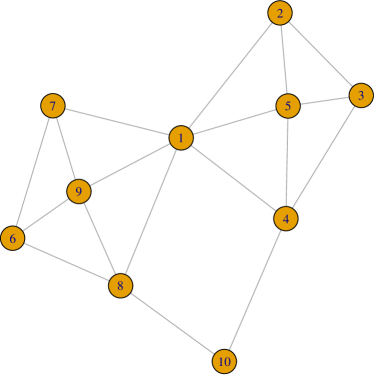
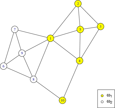
a. Original network

b. Detected communities by ELP with $\sigma^{*}$

Figure 1: A network with an outlier and a bridge.

The optimal update order of nodes by Eq. (24) is

$$\sigma^{*}=\{4,8,3,6,2,7,1,5,9,10\}.$$

The iterative update process of ELP with $\sigma^{*}$ is illustrated in Table I. Initially, each node is assigned with a unique label which is the same as its ID. And then the nodes update their own labels orderly. The $i^{\text{th}}$ column of the table shows the label of each node after the $i^{\text{th}}$ update step. The bold element of each column in the table indicates the node whose label is updated in this step. As can be seen, the nodes located in the border are updated first. Based on the definition of node influence and the label propagation strategy, the labels of central nodes are more easily adopted by the border nodes. If the update order is set to be $\sigma^{*}$, the obtained hard partition is as that shown in Fig. 1–b. The corresponding basic belief assignments for each node are shown in Fig. 2–a. As can be seen from the figure, the masses of node 1 assigned to the two communities are equal, indicating that node 1 serves as a bridge in the network. For node 10, the maximum mass is given to the ignorant set $\Omega$. Here $\Omega$ is the set for outliers which are very different from their neighbors. From the original graph, we can see that node 10 has two neighbors, nodes 4 and 8. But neither of them shares a common neighbor with node 10. Therefore, node 10 can be regarded as an outlier of the graph. From the mass assignments, it is easy to see that the plausibilities of nodes 1 and 10 for two communities are equal. Consequently it is difficult to determine their specific domain labels.

TABLE I: The iterative update process of ELP.

	0	1	2	3	4	5	6	7	8	9	10
1	1	1	1	1	1	1	1	5	5	5	5
2	2	2	2	2	2	5	5	5	5	5	5
3	3	3	3	5	5	5	5	5	5	5	5
4	4	5	5	5	5	5	5	5	5	5	5
5	5	5	5	5	5	5	5	5	5	5	5
6	6	6	6	6	9	9	9	9	9	9	9
7	7	7	7	7	7	7	9	9	9	9	9
8	8	8	9	9	9	9	9	9	9	9	9
9	9	9	9	9	9	9	9	9	9	9	9
10	10	10	10	10	10	10	10	10	10	10	5

In ELP, pignistic probabilities can also be obtained as a by-product, which can be regarded as fuzzy memberships of nodes. From Fig. 2–b we can see that both node 1 and node 10 have similar memberships for the two communities. But the positions of the two nodes in the graph are different. Node 1 is in the central part while node 10 is in the border. This is the deficiency brought by the restriction that the probabilities over the frame should be sum to 1. Consequently, it could not distinguish outliers from overlapping nodes. Although the mass values assigned to the two communities are also equal, but those to set $\Omega$ are different. The mass given to $\Omega$ for node 1 is almost 0 while for node 10 it is approaching to 1. It illustrates one of the advantages of ELP that the overlapping nodes and outliers can be detected simultaneously with the help of bbas. For one node, if the maximal mass is given to the ignorant set $\Omega$, it is likely to be an outlier. On the contrary, when a node has large equal mass assignments for more than one community, it probably locates in the overlap.

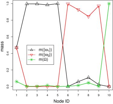
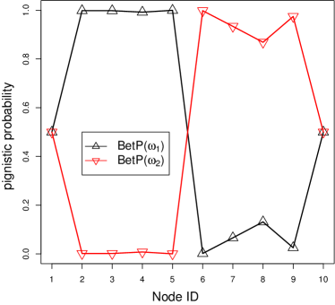
a. Mass assignments

b. Pignistic probabilities

Figure 2: The bba and pignistic probabilities of each node by ELP.

We evoke LPA many times on this simple graph. Nodes 1 and 10 are divided into different communities in different runs. LPA could detect neither the overlapping nodes nor the outliers. Before applying E$K$-NNclus algorithm, the number of nearest neighbors, $K$, should be fixed. The results by E$K$-NNclus with $K=3$ and $K=4$ are shown in Tables II and III respectively. It can be seen that five communities are detected by E$K$-NNclus. Nodes 10 and 6 are specially partitioned into two special small groups respectively. Node 1 is regarded as an outlier when $K=3$, while no outlier is detected when $K=4$. In graphs, different nodes have different number of neighbors, thus it is not reasonable to use the same $K$ for all the nodes. This may be the reason that the performance of E$K$-NNclus is not as good as that of ELP. The NMI values are not listed in this experiment as there is no ground-truth for this illustrative graph.

TABLE II: The Mass Assignment by E$K$-NNclus with $K=3$.

	1	2	3	4	5	6	7	8	9	10
$m(\{\omega_{1}\})$	0.2600	0.0000	1.0000	0.0000	0.2588	0.0000	0.0000	0.1689	0.3261	0.0000
$m(\{\omega_{2}\})$	0.1098	1.0000	0.0000	0.8159	0.5767	0.0000	0.0000	0.1689	0.0000	0.0000
$m(\{\omega_{3}\})$	0.2600	0.0000	0.0000	0.0000	0.0000	1.0000	0.0000	0.0000	0.2091	0.0000
$m(\{\omega_{4}\})$	0.0000	0.0000	0.0000	0.1021	0.0000	0.0000	1.0000	0.5265	0.2576	0.0000
$m(\{\omega_{5}\})$	0.0000	0.0000	0.0000	0.0000	0.0000	0.0000	0.0000	0.0000	0.0000	1.0000
$m(\Omega)$	0.3702	0.0000	0.0000	0.0821	0.1644	0.0000	0.0000	0.1358	0.2072	0.0000

TABLE III: The Mass Assignment by E$K$-NNclus with $K=4$.

	1	2	3	4	5	6	7	8	9	10
$m(\{\omega_{1}\})$	0.4190	0.0000	1.0000	0.2624	0.4951	0.0000	0.0000	0.0246	0.2162	0.0000
$m(\{\omega_{2}\})$	0.0000	1.0000	0.0000	0.4772	0.4171	0.0000	0.0000	0.0944	0.0000	0.0000
$m(\{\omega_{3}\})$	0.2265	0.0000	0.0000	0.0000	0.0000	1.0000	0.0000	0.0000	0.1411	0.0000
$m(\{\omega_{4}\})$	0.1016	0.0000	0.0000	0.1579	0.0000	0.0000	1.0000	0.8197	0.5309	0.0000
$m(\{\omega_{5}\})$	0.0000	0.0000	0.0000	0.0000	0.0000	0.0000	0.0000	0.0000	0.0000	1.0000
$m(\Omega)$	0.2530	0.0000	0.0000	0.1024	0.0878	0.0000	0.0000	0.0613	0.1118	0.0000

Example 2. Here we test on a widely used benchmark in detecting community structures, “Karate Club”, studied by Wayne Zachary [22]. The network consists of 34 nodes and 78 edges representing the friendship among the members of the club (see Fig. 3). During the development, a dispute arose between the club’s administrator and instructor, which eventually resulted in the club split into two smaller clubs (one marked with pink squares, and the other marked with yellow circles), centered around the administrator and the instructor respectively.

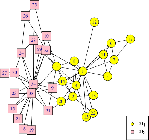
Figure 3: Karate Club network.

Let $\eta=1$, and evoke ELP many times with different update order $\sigma$s. We find that we can get two different results. Most of the time, ELP could detect two communities and find two outliers. The bbas of nodes in the two groups are illustrated in Figs. 5–a and 5–b respectively. It is showed in the figures that this network has strong class structures, since for each node the mass values assigned to different classes are significantly different. Nodes 10 and 12 are two outliers in their own communities. From the original graph, node 12 only connects with node 1. For node 10, it has two neighbors, nodes 3 and 34, but it has no connection with the neighbors of the two nodes. Neither node 10 nor node 12 has close relationship with other nodes in the network. Therefore, it is very intuitive that they are detected as outliers. It is noted here that with update order $\sigma^{*}$, we can get the above clustering result with two communities and two outliers.

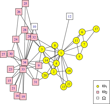
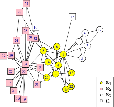
a. Two detected communities

b. Three detected communities

Figure 4: The detected communities of Karate Club network by ELP.

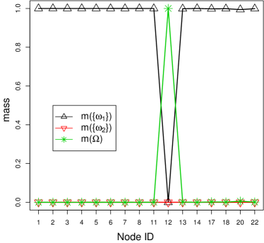
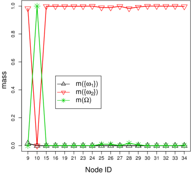
a. Community $\omega_{1}$

b. Community $\omega_{2}$

Figure 5: The bba of each node for Karate Club network by ELP.

With some $\sigma$s, a special small community can been found by ELP. As shown in Fig. 4–b, a group containing nodes 5, 6, 7, 11, 17 has been separated from community $\omega_{1}$. This seems reasonable as these nodes have no connections with other nodes in class $\omega_{1}$ except the central node (node 1). The bbas of these five nodes are illustrated in Fig. 6. It can be seen that nodes 5 and 11 have large mass values for community $\omega_{1}$ and $\omega_{3}$, which can be regarded as bridges of the two communities. Nodes 10 and 12 are still regarded as outliers in this case.

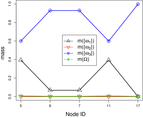
Figure 6: The bbas of the nodes in small communities Karate Club network.

To compare the accuracy and robustness of different methods, each algorithm (ELP, LPA and E$K$-NNclus with $K$ = 3, 4, 5, 6) is repeated 50 times with a random update order each time. The minimum, maximum, average and the standard deviation of NMI values are listed in Table IV. To get NMI values of the detected results of ELP, we should get the domain label of each node by assigning each node to the community with maximum plausibility. It should be noted that node 10 has a equal plausibility for community $\omega_{1}$ and $\omega_{2}$, that is,

$$pl(\omega_{1})=pl(\omega_{2}).$$

We randomly set a label as its dominant label. From the table we can find that ELP has good robustness as well as accuracy. E$K$-NNclus is stable when $K$ is relatively large, but the accuracy is not as good as that in ELP. The performance of LPA is worst in terms of stability and average accuracy.

TABLE IV: The NMI values for the detected results by different methods on Karate Club network.

			E$K$-NNclus
	ELP	LPA	$K=3$	$K=4$	$K=5$	$K=6$
Max	1.0000	1.0000	0.4648	0.4832	0.5248	0.5248
Min	0.8255	0.0000	0.4149	0.4149	0.5248	0.5248
Average	0.9314	0.6679	0.4498	0.4711	0.5248	0.5248
Deviation	0.0815	0.1945	0.0231	0.0262	0.0000	0.0000

Example 3. The network we investigate in this experiment is the world of American college football games between Division IA colleges during regular season Fall 2000. The vertices in the network represent 115 teams, while the links denote 613 regular-season games between the two teams they connect. The teams are divided into 12 conferences containing around 8-12 teams each and generally games are more frequent between members from the same conference than between those from different conferences. The original network is displayed in Fig. 7–a.

Each of the algorithms ELP, LPA, and E$K$-NNclus is repeated 50 times with different update order $\sigma$s, the statistical properties of the corresponding NMI values are listed in Table V. As can be seen, the maximal value of NMI is almost the same by LPA and ELP. However, the minimum and average by ELP are significantly larger than those by LPA. These results further demonstrate the robustness of ELP.

TABLE V: The NMI values for the detected results by different methods on Football network.

			E$K$-NNclus
	ELP	LPA	$K=3$	$K=4$	$K=5$	$K=6$
Max	0.9269	0.9269	0.8376	0.8730	0.9030	0.9030
Min	0.8892	0.8343	0.8024	0.8103	0.8404	0.8688
Average	0.9061	0.8887	0.8166	0.8384	0.8700	0.8860
Deviation	0.0080	0.0232	0.0104	0.0141	0.0139	0.0092

Now we fix the update order and let $\sigma=\sigma^{*}$. The NMI value of the detected communities is 0.9102. It is very close to the maximum 0.9269. The clustering result of ELP with $\sigma^{*}$ is presented in Fig. 7–b. As shown in the figure, six conferences are exactly identified.

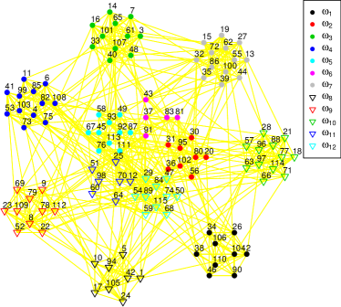
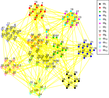
a. Original network

b. The detected communities

Figure 7: American football network.

Example 4. In this experiment, we will test on three other real-world graphs: Dolphins network, Lesmis network and Political books network [22]. For one data set, each algorithm is evoked 50 times with a random $\sigma$ each time. The statistical characteristics of the evaluation results in terms of NMI on the three data sets are illustrated in Tables VI – VIII respectively. As shown in the tables, ELP is much more stable than other approaches as the standard deviation is quite small. The average performance of ELP is best among all the methods.

TABLE VI: The NMI values for the detected results by different methods on Dolphin network.

			E$K$-NNclus
	ELP	LPA	$K=3$	$K=4$	$K=5$	$K=6$
Max	0.8230	1.0000	0.4975	0.5400	0.6729	0.6089
Min	0.5815	0.4689	0.4835	0.4786	0.5371	0.4774
Average	0.6346	0.6450	0.4964	0.5034	0.5834	0.5268
Deviation	0.0504	0.1113	0.0038	0.0205	0.0549	0.0541

TABLE VII: The NMI values for the detected results by different methods on Lesmis network.

			E$K$-NNclus
	ELP	LPA	$K=3$	$K=4$	$K=5$	$K=6$
Max	0.8645	0.8441	0.1475	0.1475	0.5357	0.5357
Min	0.8645	0.5114	0.1055	0.1055	0.4153	0.4254
Average	0.8645	0.6907	0.1190	0.1374	0.4963	0.5122
Deviation	0.0000	0.0705	0.0198	0.0181	0.0429	0.0306

TABLE VIII: The NMI values for the detected results by different methods on Books network.

			E$K$-NNclus
	ELP	LPA	$K=3$	$K=4$	$K=5$	$K=6$
Max	0.5751	0.5979	0.4348	0.4111	0.4421	0.4563
Min	0.4979	0.4607	0.4348	0.4111	0.4421	0.4563
Average	0.5496	0.5535	0.4348	0.4111	0.4421	0.4563
Deviation	0.0129	0.0333	0.0000	0.0000	0.0000	0.0000

V Conclusion

In this paper, a new community detection approach, named ELP, is presented. The proposed approach is inspired from the conventional LPA and E$K$-NNclus clustering algorithm. By the introduction of node influence, a new evidential label propagation strategy is devised. After the propagation process, the domain label of each node is determined according to its plausibilities. The experimental results illustrate the advantages of ELP. It can be used to detect the overlapping nodes and outliers at the same time. To define the influence of each node, different similarity measures can be adopted. Specially, if there are some attributes describing the features of nodes, a similarity index considering both the topological graph structure and the attribute information is a better choice. Therefore, we intend to discuss the effects of different similarity measures on ELP and the application of ELP on graphs with attribute information in our future research work.

References

- [1] M. E. Newman and M. Girvan, “Finding and evaluating community structure in networks,” Physical review E, vol. 69, no. 2, p. 026113, 2004.
- [2] S. Fortunato and M. Barthelemy, “Resolution limit in community detection,” Proceedings of the National Academy of Sciences, vol. 104, no. 1, pp. 36–41, 2007.
- [3] P. Kim and S. Kim, “Detecting overlapping and hierarchical communities in complex network using interaction-based edge clustering,” Physica A: Statistical Mechanics and its Applications, vol. 417, pp. 46–56, 2015.
- [4] M. E. Newman, “Spectral methods for community detection and graph partitioning,” Physical Review E, vol. 88, no. 4, p. 042822, 2013.
- [5] K. Zhou, A. Martin, and Q. Pan, “A similarity-based community detection method with multiple prototype representation,” Physica A: Statistical Mechanics and its Applications, vol. 438, pp. 519–531, 2015.
- [6] U. N. Raghavan, R. Albert, and S. Kumara, “Near linear time algorithm to detect community structures in large-scale networks,” Physical Review E, vol. 76, no. 3, p. 036106, 2007.
- [7] G. Shafer, A mathematical theory of evidence. Princeton University Press, 1976.
- [8] T. Denœux, “A -nearest neighbor classification rule based on dempster-shafer theory,” Systems, Man and Cybernetics, IEEE Transactions on, vol. 25, no. 5, pp. 804–813, 1995.
- [9] Z.-g. Liu, Q. Pan, G. Mercier, and J. Dezert, “A new incomplete pattern classification method based on evidential reasoning,” Cybernetics, IEEE Transactions on, vol. 45, no. 4, pp. 635–646, 2015.
- [10] M.-H. Masson and T. Denœux, “ECM: An evidential version of the fuzzy -means algorithm,” Pattern Recognition, vol. 41, no. 4, pp. 1384–1397, 2008.
- [11] K. Zhou, A. Martin, Q. Pan, and Z.-G. Liu, “Evidential relational clustering using medoids,” in Information Fusion (Fusion), 2015 18th International Conference on. IEEE, 2015, pp. 413–420.
- [12] K. Zhou, A. Martin, Q. Pan, and Z.-g. Liu, “ECMdd: Evidential -medoids clustering with multiple prototypes,” Pattern Recognition, doi: 10.1016/j.patcog.2016.05.005, 2016.
- [13] D. Wei, X. Deng, X. Zhang, Y. Deng, and S. Mahadevan, “Identifying influential nodes in weighted networks based on evidence theory,” Physica A: Statistical Mechanics and its Applications, vol. 392, no. 10, pp. 2564–2575, 2013.
- [14] K. Zhou, A. Martin, and Q. Pan, “Evidential communities for complex networks,” in Information Processing and Management of Uncertainty in Knowledge-Based Systems. Springer, 2014, pp. 557–566.
- [15] K. Zhou, A. Martin, Q. Pan, and Z.-g. Liu, “Median evidential -means algorithm and its application to community detection,” Knowledge-Based Systems, vol. 74, pp. 69–88, 2015.
- [16] T. Denœux, “Maximum likelihood estimation from uncertain data in the belief function framework,” Knowledge and Data Engineering, IEEE Transactions on, vol. 25, no. 1, pp. 119–130, 2013.
- [17] K. Zhou, A. Martin, and Q. Pan, “Evidential-EM algorithm applied to progressively censored observations,” in Information Processing and Management of Uncertainty in Knowledge-Based Systems. Springer, 2014, pp. 180–189.
- [18] P. Smets, “Decision making in the TBM: the necessity of the pignistic transformation,” International Journal of Approximate Reasoning, vol. 38, no. 2, pp. 133–147, 2005.
- [19] T. Denœux, O. Kanjanatarakul, and S. Sriboonchitta, “EK-NNclus: A clustering procedure based on the evidential -nearest neighbor rule,” Knowledge-Based Systems, vol. 88, pp. 57–69, 2015.
- [20] K. Liu, J. Huang, H. Sun, M. Wan, Y. Qi, and H. Li, “Label propagation based evolutionary clustering for detecting overlapping and non-overlapping communities in dynamic networks,” Knowledge-Based Systems, vol. 89, pp. 487–496, 2015.
- [21] L. Danon, A. Diaz-Guilera, J. Duch, and A. Arenas, “Comparing community structure identification,” Journal of Statistical Mechanics: Theory and Experiment, vol. 2005, no. 09, p. P09008, 2005.
- [22] “The UCI network data repository,” http://networkdata.ics.uci.edu/index.php.