Open-Set Support Vector Machines

Abstract

Often, when dealing with real-world recognition problems, we do not need, and often cannot have, knowledge of the entire set of possible classes that might appear during operational testing. In such cases, we need to think of robust classification methods able to deal with the “unknown” and properly reject samples belonging to classes never seen during training. Notwithstanding, existing classifiers to date were mostly developed for the closed-set scenario, i.e., the classification setup in which it is assumed that all test samples belong to one of the classes with which the classifier was trained. In the open-set scenario, however, a test sample can belong to none of the known classes and the classifier must properly reject it by classifying it as unknown. In this work, we extend upon the well-known Support Vector Machines (SVM) classifier and introduce the Open-Set Support Vector Machines (OSSVM), which is suitable for recognition in open-set setups. OSSVM balances the empirical risk and the risk of the unknown and ensures that the region of the feature space in which a test sample would be classified as known (one of the known classes) is always bounded, ensuring a finite risk of the unknown. In this work, we also highlight the properties of the SVM classifier related to the open-set scenario, and provide necessary and sufficient conditions for an RBF SVM to have bounded open-space risk.

I Introduction

Machine learning literature is rich with works proposing classifiers for closed-set pattern recognition, with well-known examples including $k$-Nearest Neighbors [$k$NN; 1], Random Forests [2], SVM, and deep neural networks [DNNs; 4]. These classifiers were inherently designed to work in closed-set scenarios, i.e., scenarios in which all test samples must belong to a class used in training. What happens when the test sample belongs to a class not seen at training time? Consider a digital forensic scenario—e.g., source-camera attribution [5], printer identification [6]—in which law officials want to verify that a particular artifact (e.g., a digital photo or a printed page) did originate from one of a few suspect devices. The suspected devices are the classes of interest, and a classifier can be trained on many examples of artifacts from these devices and from other non-suspected devices. When assigning the source for the particular artifact in question, the classifier must be aware that if the artifact is from an unknown region of the feature space—possibly far away from the training data—it cannot be assigned to one of the suspected devices, even if examples of those devices are the closest to the artifact. The classifier must be allowed to declare that the example does not belong to any of the classes it was trained on.

One possible way to address recognition in an open-set scenario is to use a closed-set classifier, obtain a similarity score—or simply the distance in the feature space—to the most likely class, apply a threshold on that similarity score aiming at classifying as unknown any test sample whose similarity score is below a specified threshold [7, 8, 9]. Mendes Júnior et al. [10] showed that when applying thresholds to the ratio of distances instead of distance themselves results in better performance in open-set scenarios. Furthermore, recent works have shown theoretical and experimental inconsistencies on employing thresholded softmax probability scores of neural networks for open-set rejection in face recognition problems [11, 12].

Instead of using similarity-based algorithms, another alternative is to exploit kernel-based algorithms such as Support Vector Data Description [SVDD; 13, 14] and one-class classifiers [15]—applied to the entire training set as a rejection function [16]. This approach is sometimes called classification with abstention. The idea is to have an initial rejection phase that predicts if the input belongs to one of the training classes or not (known or unknown). In the former case, a second phase is performed with any sort of multiclass classifier aiming at choosing the correct class.

Another alternative method relies on having a binary rejection function for each of the known classes such that a test sample is classified as unknown when decisions are negative for every function. This is the case for any multiclass-from-binary classifier based on the one-vs-all approach [17]. Some recent works have explored this idea [18, 5, 19, 20] making efforts at minimizing the positively labeled open space (PLOS) for every classifier that composes the multiclass-from-binary one. In binary classification, PLOS refers to the open space that receives positive classification. Open space is the region of the feature space outside the support of the training samples [21]. In the multiclass level, a similar concept applies: known labeled open space (KLOS), i.e., the region of the feature space outside the support of the training samples in which a test sample would be classified as one of the known classes [10]. In this class of methods, the potential of binary methods can be highly explored to multiclass open-set scenarios. Furthermore, methods in this class can be adapted for multiple class recognition in open-set scenarios, as accomplished by Heflin et al. [22].

In this work, we propose the Open-Set Support Vector Machines (OSSVM), that falls into the last class of methods and receives its name due to its ability to bound the PLOS for every classification in the binary level, consequently, bounding KLOS as well—when one-vs-all is applied. OSSVM relies on the optimization of the bias term with Radial Basis Function (RBF) kernel taking advantage of the following property we demonstrate in this work: SVM with RBF kernel bounds the PLOS if and only if the bias term is negative.

Along with this work, we have evaluated multiple implementations of open-set methods for different datasets. For all those methods we have employed the open-set grid search, as it was showed by Mendes Júnior et al. [23] that it works better over the traditional form of grid search in open-set scenarios.

The remaining of this work is organized as follows. In Section II, we discuss some of the most important previous work in open-set recognition. In Section III, we introduce the OSSVM while, in Section IV, we present the experiments that validate the proposed method. Finally, in Section V, we present the conclusions and future work.

II Related Work

In this section, we review recent works that explicitly deal with open-set recognition in the literature, including some base works for them. We note that other insights presented in many existing works can be somehow extended to be employed for the open-set scenario. Most of those works, however, did not perform the experiments with appropriate open-set recognition setup.

Heflin et al. [22] and Pritsos and Stamatatos [18] presented a multiclass SVM classifier based on the OCSVM. For each of the training classes, they fit an OCSVM. In the prediction phase, all $n$ OCSVMs classify the test sample, in which $n$ is the number of available classes for training. The test sample is classified as the class in which its OCSVM classified as positive. When no OCSVM classifies the test sample as positive, it is classified as unknown. Heflin et al. [22] extends the idea to multiple class classification, by allowing more than one OCSVMs to classify the example as positive; in this case, the example receives as labels all classes whose corresponding OCSVMs classify it as positive. Differently, Pritsos and Stamatatos [18] choose the more confident classifier among the ones that classify as positive. In those works, OCSVM is used with the RBF kernel, which allows bounding the KLOS.

Support Vector Data Description [SVDD; 13, 14] was proposed for data domain description, which means it is targeted to classify the input as belonging to the dataset or not (known or unknown). In general, any one-class or binary classifier can be applied in such cascade approach to reject or accept the test sample as belonging to one of the known classes and further defining which class it is. It is similar to the framework proposed by Cortes et al. [16] in which a rejection function is trained along with a classifier, however, in open-set scenario the classifier should be multiclass. For the case in which the rejection function accepts a sample, any multiclass classifier can be applied to choose the correct class. In case of rejection, samples are classified as unknown.

Costa et al. [24, 5] proposed the Decision Boundary Carving (DBC), an extension of the SVM classifier aiming at a more restrictive specialization on the positive class of the binary classifier. For this purpose, they move the hyperplane a value $\epsilon$ towards the positive class (in rare cases backwards). The value $\epsilon$ is obtained by minimizing the training data error. For multiclass classification, the one-vs-all approach can be employed and DBC uses the RBF kernel. Despite the specialized approach towards the positive class, DBC cannot ensure a bounded PLOS.

Scheirer et al. [21] formalized the open-set recognition problem and proposed an extension upon the SVM classifier called 1-vs-Set Machine (1VS). Similar to the works of Costa et al. [24, 5], they move the main hyperplane either direction depending on the open-space risk. In addition, a second hyperplane, parallel to the main one, is created such that the positive class is between the two hyperplanes. This second hyperplane allows the samples “behind” the positive class to be classified as negative. Then a refinement step is performed on both hyperplanes to balance open-space risk and empirical risk. According to the authors, the method works better with the linear kernel, as the second plane does not provide much benefit for an RBF kernel which has a naturally occurring upper bound. A one-vs-all approach is used to combine the binary classifiers for open-set multiclass classification.

Scheirer et al. [19] proposed the Weibull-calibrated Support Vector Machines (WSVM). The authors proposed the Compact Abating Probability (CAP) model which decreases the probability of a test sample to be considered as belonging to one of the known classes when it is far away from the training samples. They use two stages for classification: a CAP model based on a one-class classifier followed by a binary classifier with normalization based on Extreme Value Theory (EVT). The binary classifier seeks to improve discrimination and its normalization has two steps. The first aims at obtaining the probability of a test sample to belong to a positive/known class and the second step estimates the probability of it not being from the negative classes. Product of both probabilities is the final probability of the test sample to belong to a positive/known class. WSVM uses the RBF kernel and also the one-vs-all approach and ensures a bounded KLOS due to its one-class model.

Jain et al. [20] proposed the Support Vector Machines with Probability of Inclusion (PISVM), also based on the EVT. It is an algorithm for estimating the unnormalized posterior probability of class inclusion. For each known class, a Weibull distribution [25] is estimated based on the smallest decision values of the positive training samples. The binary classifier for each class is an SVM with RBF kernel trained using the one-vs-all approach, i.e., the samples of all remaining classes are considered as negative samples. They introduce the idea of cross-class validation which is similar to the open-set grid search formalized by Mendes Júnior et al. [23]. For a test sample, PISVM chooses the class for which the decision value produces the maximum probability of inclusion. If that maximum is below a given threshold, the input is marked as unknown. PISVM is not able to ensure a bounded PLOS and, consequently, nor the KLOS.

Also applying EVT, Rudd et al. [26] proposed a method purely based on Weibull extreme value distributions, named the Extreme Value Machine (EVM). Their method generates a distribution for each of the known instances aiming at a separation from instances of other classes. In a later step, those distributions are summarized aiming at a tight probabilistic representation for each of the known classes. Test phase comprises the verification of pertinence to each of those distributions and examples are rejected when they are outliers for every distribution. As EVM creates CAP models, it is able to bound the KLOS.

Applying EVT in open-set recognition has been a recent research focus. Scheirer [27] presents an overview of how EVT have been recently applied to visual recognition, mainly on the context of open-set recognition. Notice that some of the previous EVT-based works are not capable of ensuring a bounded KLOS by solely relying on EVT models. In the case of Scheirer et al. [19], they ensure bounded KLOS based on one-class models but not on EVT models. For PISVM [20], the authors did not prove their method is able to bound KLOS. In fact, PISVM can leave an unbounded KLOS when the value of the bias term of the SVM model is in the range of scores used to fit the Weibull model. As EVT for open-set recognition is a growing research area, we highlight that one advantage of our proposed method, compared to EVT-based ones, relies on its simplicity. The proposed method is defined purely as a convex optimization problem, as it is for SVM. EVT-based methods require post-processing after an SVM model is trained, or—as it is the case of EVM—it requires an expensive model calculated per training instance. At testing phase, our proposed method requires just the prediction from the obtained SVM model, while SVM- and EVT-based methods require extra predictions from EVT models for each binary classifier that composes the multiclass one.

Mendes Júnior et al. [10] have shown that thresholding ratio of distances in the feature space for a nearest neighbor classifier is more accurate at predicting unknown samples in an open-set problem. The effectiveness of working with ratio of decision scores is confirmed by Vareto et al. [28], in which one of the best rejection threshold estimated for a face-recognition problem is established based on the ratio of the two highest scores obtained by a voting from a set of binary classifiers.

It is worth noticing that well-known machine learning areas have been investigated from the point of view of the open-set scenario, e.g., domain adaptation [29, 30, 31, 32], genetic programming [33], object detection [34], incremental learning [35], etc., taking into account particularities from open-set recognition. Beyond those methods specifically proposed for open-set setups, many other solutions in literature can be investigated to be extended for open-set scenarios. In general, any binary classification method that aims at decreasing false positive rate [36] would potentially recognize unknown samples when composing such classifiers with one-vs-all approach.

In general, recent solutions for open-set recognition problems have focused on methods that use samples of all known classes for training models for individual classes. That is different from generative approaches that checks if the test sample is in the distribution of each of the known classes, as it tries to use data from all classes for generating the model for each class. It differs from reject option [37, 38] in the sense that we do not want just to postpone decision making. Moreover, open-set recognition differs from domain adaptation and from transfer learning in the sense that transferring knowledge from one domain to another does not ensure the ability of identifying samples belonging to unknown classes.

Also, multiple researches have been recently accomplished considering open-set recognition for multiple applications, e.g., audio recognition [39], user identity verification [40], camera model identification [23], human activity recognition [41], etc. Geng et al. [42] present a survey of the literature on open-set recognition; we refer the reader to their work for a more complete review of the literature.

III Open-Set Support Vector Machines

One cannot ensure that the positive class of the traditional SVM has a bounded PLOS, even when the RBF kernel is used. The main characteristic of the proposed OSSVM is that a high enough regularization parameter ensures a bounded PLOS for every known class of interest, consequently, a bounded KLOS in one-vs-all multiclass level. The regularization parameter is a weight for optimizing the risk of the unknown in relation to the empirical risk measured on training data. In Section III-B, we present how to ensure a bounded PLOS using RBF kernel. In Section III-C, we present the formulation of the optimization problem of the OSSVM. To begin with, in Section III-A, we present some basic aspects of the SVM classifier.

III-A Basic aspects of Support Vector Machines

SVM is a binary classifier that, given a set $X$ of training samples $\mathbf{x}_{i}\in\mathbb{R}^{d}$ and the corresponding labels $y_{i}\in\{-1,1\}$, $i=1,\dots,m$, it finds a maximum-margin hyperplane that separates $\mathbf{x}_{i}$ for which $y_{i}=-1$ from $\mathbf{x}_{j}$ for which $y_{j}=1$ [3]. We consider the soft margin case with parameter $C$.

The primal optimization problem is usually defined as

$$\min_{\mathbf{w},b,\xi}\frac{1}{2}\|\mathbf{w}\|^{2}+C\sum_{i=1}^{m}\xi_{i},$$

s.t. $$y_{i}(\mathbf{w}^{T}\mathbf{x}_{i}+b)\geq 1-\xi_{i},\ \forall i,$$ (1)

$$\xi_{i}\geq 0,\ \forall i.$$ (2)

To solve this optimization problem, we use the Lagrangian method to create the dual optimization problem. In this case, the final Lagrangian is defined as

$$\mathcal{L}(\alpha)=\sum_{i=1}^{m}\alpha_{i}-\frac{1}{2}\|\mathbf{w}\|^{2},$$ (3)

in which $\mathbf{w}=\sum_{i=1}^{m}\alpha_{i}y_{i}\mathbf{x}_{i}$ and $\alpha_{i}\in\mathbb{R}$, $i=1,\dots,m$, are the Lagrangian multipliers. Then, the optimization problem now is defined as

$$\min_{\alpha}\ \mathcal{W}(\alpha)=-\mathcal{L}(\alpha)=\frac{1}{2}\|\mathbf{w}\|^{2}-\sum_{i=1}^{m}\alpha_{i},$$ (4)

s.t. $$0\leq\alpha_{i}\leq C,\ \forall i,$$ (5)

$$\sum_{i=1}^{m}\alpha_{i}y_{i}=0.$$ (6)

The decision function of a test sample $\mathbf{x}$ comes from the constraint in Equation (1) and is defined as

$$f(\mathbf{x})=\operatorname{sign}(\mathbf{w}^{T}\mathbf{x}+b)=\operatorname{sign}\left(\sum_{i=1}^{m}y_{i}\alpha_{i}\mathbf{x}_{i}^{T}\mathbf{x}+b\right).$$ (7)

Boser et al. [43] proposed a modification in SVM for the cases in which the training data are not linearly separated in the feature space. Instead of linearly separating the samples in the original space $\mathcal{X}$ of the training samples in $X$, the samples are projected onto a higher dimensional space $\mathcal{Z}$ in which they are linearly separated. This projection is accomplished using the kernel trick [44]. One advantage of this method is that in addition to separating non-linear data, the optimization problem of the SVM remains almost the same: instead of calculating the inner product $\mathbf{x}^{T}\mathbf{x}^{\prime}$, it uses a kernel $K(\mathbf{x},\mathbf{x}^{\prime})$ that is equivalent to the inner product $\phi(\mathbf{x})^{T}\phi(\mathbf{x}^{\prime})$ in a higher dimensional space $\mathcal{Z}$, in which $\phi:\mathcal{X}\mapsto\mathcal{Z}$ is a projection function. When using the kernel trick, we do not need to know the $\mathcal{Z}$ space explicitly.

Using kernels, the decision function of a test sample $\mathbf{x}$ becomes

$$f(\mathbf{x})=\operatorname{sign}\left(\sum_{i=1}^{m}y_{i}\alpha_{i}K(\mathbf{x}_{i},\mathbf{x})+b\right).$$ (8)

The most used kernel for SVM is the RBF kernel [45], defined as follows.

$$K(\mathbf{x},\mathbf{x}^{\prime})=e^{-\gamma\|\mathbf{x}-\mathbf{x}^{\prime}\|^{2}}.$$ (9)

It is proved that using this kernel, the projection space $\mathcal{Z}$ is an $\infty$-dimensional space [45].

III-B Ensuring a bounded PLOS

By simply employing the RBF kernel, we cannot ensure the PLOS is bounded.

Theorem 1.

SVM with RBF kernel has a bounded positively labeled open space (PLOS) if and only if the bias term $b$ is negative.

Proof.

We know that

$$\lim_{d\rightarrow\infty}K(\mathbf{x},\mathbf{x}^{\prime})=0,$$ (10)

in which $K(\mathbf{x},\mathbf{x}^{\prime})$ is the RBF kernel and $d=\|\mathbf{x}-\mathbf{x}^{\prime}\|$. For the cases in which a test sample $\mathbf{x}$ is far away from every support vector $\mathbf{x}_{i}$, we have that

$$\sum_{i=1}^{m}y_{i}\alpha_{i}K(\mathbf{x}_{i},\mathbf{x})$$

also tends to 0. From Equation (8) it follows that

$$f(\mathbf{x})=\operatorname{sign}\left(b\right)$$

when $\mathbf{x}$ is far away from the support vectors. Therefore, for negative values of $b$, $f(\mathbf{x})$ is always negative for far away $\mathbf{x}$ samples. That is, samples in a bounded region of the feature space will be classified as positive. For the only if direction, let $b$ be positive. Then, for far away $\mathbf{x}$ examples we have $f(\mathbf{x})=\operatorname{sign}(b)>0$, i.e., positively classified samples will be in an unbounded region of the feature space when $b$ is positive. ∎

Theorem 1 can be applied not only to the RBF kernel of Equation (9) but to any radial basis function [47] kernel satisfying Equation (10), e.g., Generalized T-Student kernel, Rational Quadratic kernel, and Inverse Multiquadric kernel [48], however, for the remaining part of this work, we focus on the RBF kernel of Equation (9).

Figure 4 depicts the rationale behind Theorem 1 on a 2-dimensional synthetic dataset. The $z$ axis represents the decision values for which possible 2-dimensional test samples $(x,y)$ would have for different regions of the feature space. Training samples are normalized between 0 and 1. Note in the subfigures that for possible test samples far away from the training ones, e.g., $(2,2)$, the decision value approaches the bias term $b$. Note in Figure LABEL:fig:figPlottingkernel3d__boat_forboundaries__cls03__01__gammaexp+04 that an unbounded region of the feature space would have samples classified as positive. Consequently, all those samples would be classified as class 3 by the final multiclass-from-binary classifier. In general SVM usage, both positive and negatives biases occur as $b$ depends on the training data.

In case of SVM s without explicit bias term [49, 50], $b=0$ is implicit. Consequently, the decision function is defined as

$$f(\mathbf{x})=\operatorname{sign}\left(\sum_{i=1}^{m}y_{i}\alpha_{i}K(\mathbf{x}_{i},\mathbf{x})\right).$$

For test samples far away from the support vectors, we have that $\sum_{i=1}^{m}y_{i}\alpha_{i}K(\mathbf{x}_{i},\mathbf{x})$ converges to 0 from the bottom or from the above, depending on the training samples. Consequently, a bounded PLOS cannot be ensured in all cases.

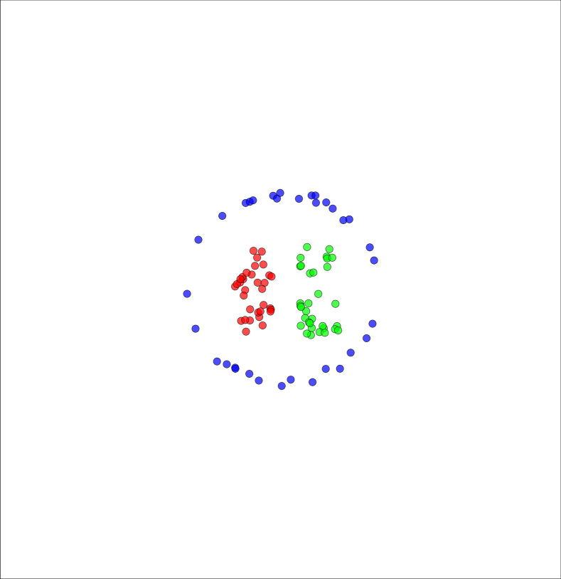
Boat dataset with 3 classes: red (the central class to the left), green (the central class to the right), and blue (the class with the ring shape).

Figure 1: Class 1 (red). $b=-0.832$.

Figure 2: Class 2 (green). $b=-0.86$.

Figure 3: Class 3 (blue). $b=+0.594$.

Figure 4: Behavior of the Support Vector Machines (SVM) with a Radial Basis Function (RBF) kernel on a 2-dimensional synthetic dataset. Image on the top-left depicts the Boat dataset [51]. Figures (LABEL:fig:figPlottingkernel3d__boat_forboundaries__cls01__01__gammaexp+04)–(LABEL:fig:figPlottingkernel3d__boat_forboundaries__cls03__01__gammaexp+04) correspond to the red, green and blue classes of the Boat dataset, respectively. $x$, $y$ axes in Figures (LABEL:fig:figPlottingkernel3d__boat_forboundaries__cls01__01__gammaexp+04)–(LABEL:fig:figPlottingkernel3d__boat_forboundaries__cls03__01__gammaexp+04) represent the two features of the dataset (the dataset is normalized between 0 and 1). $z$ axis shows the value of the decision function $\sum_{i=1}^{m}y_{i}\alpha_{i}K(\mathbf{x}_{i},\mathbf{x})+b$ (Equation 8 without $\operatorname{sign}$ function) and the colored lines in the walls depict the point 0, that separates the positive class from the negative one (equivalent to the $\operatorname{sign}$ function of Equation 8). Note in Figure (LABEL:fig:figPlottingkernel3d__boat_forboundaries__cls03__01__gammaexp+04) that an unbounded region of the feature space remains in the positive side, as $b>0$ and $f(x,y)\approx b$ for ($x$, $y$) points far away from support vectors.

//in /figPlottingkernel3d__boat_forboundaries__cls01__01__gammaexp+04/, /figPlottingkernel3d__boat_forboundaries__cls02__01__gammaexp+04/, /figPlottingkernel3d__boat_forboundaries__cls03__01__gammaexp+04/

Theorem 1 also provides a solution to the problem of unbounded PLOS. We can ensure a bounded PLOS by simply employing an RBF kernel and ensuring a negative $b$. In Section III-C, we present a new SVM optimization objective that optimizes the margin while ensuring the bias term $b$ is negative.

III-C Optimization to ensure negative bias term $b$

As we discussed in Section III-B, we must ensure a negative $b$ to obtain a bounded PLOS. For this, we define the OSSVM optimization problem as

$$\min_{\mathbf{w},b,\xi}\frac{1}{2}\|\mathbf{w}\|^{2}+C\sum_{i=1}^{m}\xi_{i}+\lambda b,$$ (11)

subject to the same constraints defined in Equations (1) and (2), in which $\lambda$ is a regularization parameter that trades off between the empirical risk and the risk of the unknown.

From Equation (11), the dual formulation has the same Lagrangian defined in Equation (3). Consequently, we have to optimize the same function as defined in Equation (4) with the constraint in Equation (5). However, the constraint in Equation (6) is replaced by the constraint

$$\sum_{i=1}^{m}\alpha_{i}y_{i}=\lambda.$$ (12)

The same Sequential Minimal Optimization (SMO) algorithm proposed by Platt [52], with the Working Set Selection (WSS) proposed by Fan et al. [53], for optimizing ensuring the constraint in Equation (6) can be applied to this optimization containing the constraint of the Equation (12). As the main idea of the SMO algorithm is to ensure that $\sum\alpha_{i}y_{i}$ remains the same from one iteration to the other, before the optimization starts, we initialize $\alpha_{i}$ such that $\sum\alpha_{i}y_{i}=\lambda$. For this, we let $\alpha_{i}=\lambda/m_{p}$, $\forall i$ such that $y_{i}=1$, in which $m_{p}$ is the number of positive training samples.

Proposition 1.

For the SVM with soft margin, the maximum valid value for $\lambda$ is $Cm_{p}$.

Proof.

From Equation (5), $0\leq\alpha_{i}\leq C$. The maximum value $\lambda=\sum\alpha_{i}y_{i}$ is thus obtained by setting $\alpha_{i}=C$ for $i$ such that $y_{i}=1$ and setting $\alpha_{i}=0$ for $i$ such that $y_{i}=-1$. This yields $\lambda\leq Cm_{p}$ ∎

During optimization, we must ensure $\lambda\leq Cm_{p}$ given that if $\lambda>Cm_{p}$, the constraint in Equation (5) would be broken for some $\alpha_{i}$.

Despite Proposition 1 saying that it is allowed $\lambda=Cm_{p}$, when it happens, we have that $\alpha_{i}=C$ for $y_{i}=1$ and $\alpha_{i}=0$ for $y_{i}=-1$, and there will be no optimization. In this case, despite satisfying the constraints, there is no flexibility for changing values of $\alpha_{i}$ because, for each pair $\alpha_{i},\alpha_{j}$ selected by the WSS algorithm, we must update $\alpha_{i}=\alpha_{i}+\nabla_{\alpha}$, $\alpha_{j}=\alpha_{j}+\nabla_{\alpha}$ when $y_{i}\neq y_{j}$ and $\alpha_{i}=\alpha_{i}-\nabla_{\alpha}$, $\alpha_{j}=\alpha_{j}+\nabla_{\alpha}$ when $y_{i}=y_{j}$. For any $\nabla_{\alpha}\neq 0$, the constraint $0<\alpha_{i}<C$ would break for either $\alpha_{i}$ or $\alpha_{j}$, for any selected pair. Then, in practice, we grid search $\lambda$ in the interval $0\leq\lambda<Cm_{p}$.

Proposition 1 holds true for any kernel, however, the formulation in Equation (11) only has the open-set properties previously discussed with an RBF kernel, as we have observed through Theorem 1.

Proposition 2.

There exists some $\lambda$ such that we can obtain a bias term $b<0$ for the OSSVM with an RBF kernel $K$ such that $0<K(\mathbf{x},\mathbf{x}^{\prime})\leq 1$ when $C\geq 1$.

Proof.

From the Karush-Kuhn-Tucker [KKT; 1] conditions, the bias term is defined as

$$b =y_{i}-\sum_{j=1}^{m}\alpha_{j}y_{j}K\left(\mathbf{x}_{i},\mathbf{x}_{j}\right)$$

$$=y_{i}-\sum_{\begin{subarray}{c}j=1:\\ y_{j}=1\end{subarray}}^{m}\alpha_{j}K\left(\mathbf{x}_{i},\mathbf{x}_{j}\right)+\sum_{\begin{subarray}{c}j=1:\\ y_{j}=-1\end{subarray}}^{m}\alpha_{j}K\left(\mathbf{x}_{i},\mathbf{x}_{j}\right),$$

for any $i$ such that $0<\alpha_{i}<C$. Now, let us consider two possible cases: (1) $y_{i}=1$ and (2) $y_{i}=-1$. For Case (1), we have

$$b=1-\alpha_{i}-\sum_{\begin{subarray}{c}j=1:\\ y_{j}=1,\\ j\neq i\end{subarray}}^{m}\alpha_{j}K\left(\mathbf{x}_{i},\mathbf{x}_{j}\right)+\sum_{\begin{subarray}{c}j=1:\\ y_{j}=-1\end{subarray}}^{m}\alpha_{j}K\left(\mathbf{x}_{i},\mathbf{x}_{j}\right),$$

as $K\left(\mathbf{x}_{i},\mathbf{x}_{i}\right)=1$. Note that $0<K(\mathbf{x},\mathbf{x}^{\prime})\leq 1$. To show that there exists some $\lambda$ such that $b<0$, we analyze the worst case, i.e., when the kernel in the second summation—for negative training samples—is $1$. Then, we have

$$b=1-\alpha_{i}-\sum_{\begin{subarray}{c}j=1:\\ y_{j}=1,\\ j\neq i\end{subarray}}^{m}\alpha_{j}K\left(\mathbf{x}_{i},\mathbf{x}_{j}\right)+\sum_{\begin{subarray}{c}j=1:\\ y_{j}=-1\end{subarray}}^{m}\alpha_{j}.$$

From Equation (12), we have

$$\sum_{\begin{subarray}{c}j=1:\\ y_{j}=-1\end{subarray}}^{m}\alpha_{j}=\sum_{\begin{subarray}{c}j=1:\\ y_{j}=1\end{subarray}}^{m}\alpha_{j}-\lambda,$$ (13)

then

$$b=1-\sum_{\begin{subarray}{c}j=1:\\ y_{j}=1,\\ j\neq i\end{subarray}}^{m}\alpha_{j}K\left(\mathbf{x}_{i},\mathbf{x}_{j}\right)+\sum_{\begin{subarray}{c}j=1:\\ y_{j}=1\\ j\neq i\end{subarray}}^{m}\alpha_{j}-\lambda$$

Analyzing the worst case again, considering $\alpha_{j}=C$ for positive training samples, with $j\neq i$, we have

$$b =1-C\sum_{\begin{subarray}{c}j=1:\\ y_{j}=1,\\ j\neq i\end{subarray}}^{m}K\left(\mathbf{x}_{i},\mathbf{x}_{j}\right)+C\left(m_{p}-1\right)-\lambda$$

$$=1+Cm_{p}-C-C\sum_{\begin{subarray}{c}j=1:\\ y_{j}=1,\\ j\neq i\end{subarray}}^{m}K\left(\mathbf{x}_{i},\mathbf{x}_{j}\right)-\lambda.$$

To ensure $b<0$ it is sufficient to let

$$\lambda>1+Cm_{p}-C-C\sum_{\begin{subarray}{c}j=1:\\ y_{j}=1,\\ j\neq i\end{subarray}}^{m}K\left(\mathbf{x}_{i},\mathbf{x}_{j}\right).$$ (14)

From Proposition 1, we have that $\lambda\leq Cm_{p}$. This fact, along with Equation (14), leads to the constraint

$$1+Cm_{p}-C-C\sum_{\begin{subarray}{c}j=1:\\ y_{j}=1,\\ j\neq i\end{subarray}}^{m}K\left(\mathbf{x}_{i},\mathbf{x}_{j}\right)<Cm_{p},$$

which simplifies to

$$1-C-C\sum_{\begin{subarray}{c}j=1:\\ y_{j}=1,\\ j\neq i\end{subarray}}^{m}K\left(\mathbf{x}_{i},\mathbf{x}_{j}\right)<0.$$

Analyzing the worst case one more time, considering $K\left(\mathbf{x}_{i},\mathbf{x}_{j}\right)\approx 0$ for the positive training samples other than $\mathbf{x}_{i}$, and replacing the term with kernel summation to $\epsilon$, we have

$$1-C-\epsilon<0.$$

As $\epsilon>0$, it is always possible to satisfy this constraint for $C\geq 1$.

For Case (2), we have

$$b=-1-\sum_{\begin{subarray}{c}j=1:\\ y_{j}=1\end{subarray}}^{m}\alpha_{j}K\left(\mathbf{x}_{i},\mathbf{x}_{j}\right)+\sum_{\begin{subarray}{c}j=1:\\ y_{j}=-1\end{subarray}}^{m}\alpha_{j}K\left(\mathbf{x}_{i},\mathbf{x}_{j}\right).$$

Considering the worst case for the values of the kernel for negative samples and using the equality in Equation (13), we have

$$b=-1-\sum_{\begin{subarray}{c}j=1:\\ y_{j}=1\end{subarray}}^{m}\alpha_{j}K\left(\mathbf{x}_{i},\mathbf{x}_{j}\right)+\sum_{\begin{subarray}{c}j=1:\\ y_{j}=1\end{subarray}}^{m}\alpha_{j}-\lambda.$$

Considering the highest possible value for $b$, by setting $\alpha_{j}=C$ for positive samples, we have

$$b=-1-C\sum_{\begin{subarray}{c}j=1:\\ y_{j}=1\end{subarray}}^{m}K\left(\mathbf{x}_{i},\mathbf{x}_{j}\right)+Cm_{p}-\lambda.$$

In this case, to ensure $b<0$ it is sufficient to let

$$\lambda>Cm_{p}-1-C\sum_{\begin{subarray}{c}j=1:\\ y_{j}=1\end{subarray}}^{m}K\left(\mathbf{x}_{i},\mathbf{x}_{j}\right),$$

which is possible to obtain for any value of $C$ in such way that $\lambda\leq Cm_{p}$ of Proposition 1 is also satisfied. ∎

In Proposition 2, we considered a very extreme case for the proof. For example, in Case (1)—for $i$ such that $y_{i}=1$—we considered $K\left(\mathbf{x}_{i},\mathbf{x}_{j}\right)=1$ for $j$ such that $y_{j}=-1$ and $K\left(\mathbf{x}_{i},\mathbf{x}_{j}\right)\approx 0$ for $j$ such that $y_{j}=1,j\neq i$. It means that all negative samples have the same feature vector of sample $\mathbf{x}_{i}$ under consideration and all positive samples are far away from sample $\mathbf{x}_{i}$. In practice, we do not have the $\lambda$ nearly as constrained as in the proof to ensure a negative bias term. Moreover, in our experiments with the SVM , we observed that oftentimes the bias term is negative for a binary classifier trained with the one-vs-all approach, i.e., it is often the case that even with $\lambda=0$ the bias will be negative. More details about this behavior is shown in Section IV-F.

One can argue that instead of defining the new optimization problem of Equation (11), the SVM decision function of Equation (8) could be simply changed to

$$f(\mathbf{x})=\sum_{i=1}^{m}y_{i}\alpha_{i}K(\mathbf{x}_{i},\mathbf{x})+b>\epsilon$$ (15)

in order to bound the PLOS, in which $\epsilon$ is a parameter that could be defined after the optimization process. As Equation (15) is equivalent to

$$f(\mathbf{x})=\operatorname{sign}\left(\sum_{i=1}^{m}y_{i}\alpha_{i}K(\mathbf{x}_{i},\mathbf{x})+b-\epsilon\right),$$

the PLOS could be bounded if and only if $\epsilon\geq b$. However, this simplified approach has drawbacks. The value of $b$ can only be known after the SVM optimization process is completed and it depends on the training data. Notice that the introduction of $\epsilon$ is equivalent to performing a parallel translation of the optimal hyperplane. As SVM only optimizes the empirical risk, the final model would not be optimal neither according to the empirical risk itself nor the open-space risk. On the other hand, OSSVM optimizes both the empirical risk and the open-space risk and the separation hyperplane obtained by OSSVM is not necessarily parallel to the position of the hyperplane that would be obtained by the traditional SVM on the same training data.

In Appendix A, we present the complete formulation of the optimization problem for the OSSVM classifier.

Choosing the $\lambda$ parameter for the OSSVM

Proposition 2 states that we can find a $\lambda$ parameter that ensures a bounded PLOS for the optimization problem presented above. To ensure this, models with a non-negative bias term receive accuracy of $-\infty$ on the validation set, during the grid search. Nevertheless, we cannot ignore that, in special circumstances, certain $\lambda$ values allow a negative bias term during the grid search but not for training in the whole set of training samples. In this case, once the parameters are obtained by grid search, if the obtained $\lambda$ does not ensure a negative bias term for the whole training set, one would need to retrain the classifier with an increased value for $\lambda$, until a negative bias term is obtained for the final model. However, for grid search, we assume the distribution of the validation set, a subset of the training set, represents the distribution of the training set; that is one possible explanation as for why in our experiments we did not need to retrain the classifier with a value of $\lambda$ larger than the one obtained during grid search, as all values of $\lambda$ obtained during grid search were able to ensure a negative bias term for all binary classifiers.

In summary, OSSVM optimizes the bias term $b$ in order to ensure a bounded PLOS for every binary classifier. The PLOS is bounded if and only if $b<0$. The $\lambda$ parameter introduced by OSSVM is responsible for optimizing $b$, taking into account the risk of the unknown.

IV Experiments

In this section, we present the experiments and details for comparing the proposed method with the existing ones in the literature, discussed in Section II. In Section IV-A, we summarize the baselines. In Section IV-B, we describe the evaluation measures used in our experiments. In Section IV-C, we describe the datasets and features. In Section IV-D, we present initial results regarding the behavior of the methods in feature space. Finally, we present the results with statistical tests in Section IV-E, finishing this section with some remarks in Section IV-F.

IV-A Baselines

In this work, we employ the one-class–based method of Pritsos and Stamatatos [18] for comparison, hereinafter referred to as Multiclass One-Class Support Vector Machines (SVM${}^{\mbox{\scriptsize OC}}$). Although Pritsos and Stamatatos [18] use a OCSVM as the method to define a rejection function for each class, one could also use a Support Vector Data Description [SVDD; 13, 14], since it is also a form of one-class classifier. We also implemented this alternative to SVM${}^{\mbox{\scriptsize OC}}$ and refer to it as multiclass SVDD (SVDD${}^{\mbox{\scriptsize OC}}$).

Despite dealing with a multiclass problem, Costa et al. [24, 5] evaluated their method DBC in the binary fashion by obtaining the accuracy of individual binary classifiers. They did not present the multiclass version of the classifier directly. Therefore, in this work, we consider their method with the one-vs-all approach in the experiments. The test sample is classified as unknown when no binary classifier classifies it as positive. Complementarily, it is classified as the most confident class when one or more classifiers tags it as positive.

Besides those methods, we have employed SVM [46], 1VS [21], WSVM [19], PISVM [20], and EVM [26] as baselines for our experiments. Among those methods, only one-class–based methods, EVM and OSSVM are able to ensure a bounded KLOS. We summarize the methods in Table I.

Method		RBF	EVT	One-class	Bounded
		kernel	based	based	KLOS
SVM	Chang and Lin [46]	✓
SVM${}^{\mbox{\scriptsize OC}}$	Pritsos and Stamatatos [18]	✓		✓	✓
SVDD${}^{\mbox{\scriptsize OC}}$	Tax and Duin [13]	✓		✓	✓
DBC	Costa et al. [5]	✓
1VS	Scheirer et al. [21]
WSVM	Scheirer et al. [19]	✓	✓	✓	✓
PISVM	Jain et al. [20]	✓	✓
EVM	Rudd et al. [26]		✓		✓
OSSVM	(Proposed method)	✓			✓

TABLE I: General characteristics of the methods compared in the experiments.

We have employed the open-set grid search approach for the existing methods in the literature, as in previous work it has been demonstrated to better estimate the parameters for classifiers in open-set scenarios [23]. Except for EVM, all compared methods are SVM-based. Parameters of the proposed method and baselines were obtained through grid search. All SVM-based methods have fixed $C=1$. For RBF-based methods, the $\gamma$ parameter were searched in $\{2^{-15},2^{-13},\dots,2^{15}\}$. The $\nu$ parameter of SVM${}^{\mbox{\scriptsize OC}}$ were searched among 21 values linearly spaced in $[0,1]$. The $p_{A}$ and $p_{\Omega}$ parameters of the 1VS were both searched in $\{2^{-3},2^{-2},\dots,2^{2}\}$. The $\delta_{\tau}$ threshold for WSVM’s CAP model were fixed in 0.001, as specified by the authors [19], and the $\delta_{R}$ were searched in $\{2^{-7},2^{-6},\dots,2^{0}\}$. The PISVM’s threshold were searched among 20 values linearly spaced in $[0,1)$. The $\lambda$ parameter of OSSVM were searched among 20 values linearly spaced in $[0,Cm_{p})$.

IV-B Evaluation measures

Most of the proposed evaluation performance measures in the literature are focused on binary classification, e.g., traditional classification accuracy, f-measure, etc. [54]. Even the ones proposed for multiclass scenarios—e.g., average accuracy, multiclass f-measure, etc.—usually consider only the closed-set scenario. Recently, Mendes Júnior et al. [10] have proposed normalized accuracy (NA) and open-set f-measure (OSFM) for multiclass open-set recognition problems. In this work, we apply such measures and further extend the NA to HNA , based on the harmonic mean [55], as shown in Equation (16).

$$\lx@glossaries@gls@link{acronym}{hna}{\leavevmode\mbox{HNA}}=\begin{cases}0,\text{if }\lx@glossaries@gls@link{acronym}{aks}{\leavevmode\mbox{AKS}}=0\text{ or }\lx@glossaries@gls@link{acronym}{aus}{\leavevmode\mbox{AUS}}=0,\\ \displaystyle\frac{2}{\displaystyle\left(\frac{1}{\displaystyle\lx@glossaries@gls@link{acronym}{aks}{\leavevmode\mbox{AKS}}}+\frac{1}{\displaystyle\lx@glossaries@gls@link{acronym}{aus}{\leavevmode\mbox{AUS}}}\right)},\text{otherwise}.\end{cases}$$ (16)

In this case, AKS is the accuracy on known samples and AUS is the accuracy on unknown samples. AKS is the accuracy obtained on the testing instances that belong to one of the classes with which the classifier was trained. AUS is the accuracy on the testing instances whose classes have no representative instances in the training set.

One advantage of HNA over NA is that when a classifier performs poorly on AKS or AUS, HNA drops toward 0. One biased classifier that blindly classifies every example as unknown would receive NA of 0.5 while HNA would be 0. However, notice that 0.5 is not the worst possible accuracy for NA, as some methods—trying to correctly predict test labels—can have its NA smaller than 0.5. The worst case for NA—when it is 0—would be when all known samples are classified as unknown and all unknown samples classified as belonging to one of the known classes. On the other hand, the worst case for HNA would be when at least one of such cases happens.

For experiments in this work, we have considered NA, HNA , OSFM_M, and OSFM_μ. For a fair comparison with previous methods in the literature [21, 19, 20, 26]—which only showed performance figures using the traditional f-measure—we also present results regarding the traditional multiclass f-measure [54] considering both FM_M and FM_μ.

IV-C Datasets

For validating the proposed method and comparing it with existing methods, we consider nineteen datasets. In the 15-Scenes [56] dataset (with 15 classes), the images are represented by a bag-of-visual-word vector created with soft assignment [57] and max pooling [58], based on a codebook of 1000 Scale Invariant Feature Transform (SIFT) codewords [59]. Letter [60, 61] dataset (with 26 classes) represents the letters of the English alphabet (black-and-white rectangular pixel displays). The KDDCUP [62] dataset (with 32 classes) represents an intrusion detection problem on a military network environment and its feature vectors combine continuous and symbolic features. In the Auslan [63] dataset (with 95 classes), the data was acquired using two Fifth Dimension Technologies (5DT) gloves hardware and two Ascension Flock-of-Birds magnetic position trackers. In the Caltech-256 [64] dataset (with 256 classes), the feature vectors consider a bag-of-visual-words characterization approach, with features acquired with dense sampling, SIFT descriptor for the points of interest, hard assignment [57], and average pooling [58]. Finally, for the ALOI [65] dataset (with 1000 classes), the features were extracted with the Border/Interior (BIC) descriptor [66]. These datasets or other datasets could be used with different characterizations, however, in this work, we focus on the learning part of the problem rather than on the feature characterization one.

Dataset	# classes	# samples	# features	# samples/class
				mean	min	max
yeast	$9$	$1479$	$8$	$164.333,333$	$20$	$463$
mfeat-morphological	$10$	$2000$	$6$	$200.000,000$	$200$	$200$
mfeat-zernike	$10$	$2000$	$47$	$200.000,000$	$200$	$200$
mfeat-karhunen	$10$	$2000$	$64$	$200.000,000$	$200$	$200$
mfeat-fourier	$10$	$2000$	$76$	$200.000,000$	$200$	$200$
mfeat-factors	$10$	$2000$	$216$	$200.000,000$	$200$	$200$
led7	$10$	$3200$	$7$	$320.000,000$	$270$	$341$
led24	$10$	$3200$	$24$	$320.000,000$	$296$	$337$
optdigits	$10$	$5620$	$64$	$562.000,000$	$554$	$572$
pendigits	$10$	$10,992$	$16$	$1099.200,000$	$1055$	$1144$
CIFAR10	$10$	$50,000$	$192$	$5000.000,000$	$5000$	$5000$
MNIST	$10$	$55,000$	$1024$	$5500.000,000$	$4987$	$6179$
vowel	$11$	$990$	$13$	$90.000,000$	$90$	$90$
movement_libras	$15$	$360$	$90$	$24.000,000$	$24$	$24$
15-Scenes	$15$	$4485$	$1000$	$299.000,000$	$210$	$410$
KRKOPT	$18$	$28,056$	$6$	$1558.666,667$	$27$	$4553$
Letter	$26$	$20,000$	$16$	$769.230,769$	$734$	$813$
KDDCUP	$32$	$10,237$	$41$	$319.906,250$	$11$	$500$
Auslan	$95$	$146,949$	$22$	$1546.831,579$	$1390$	$1938$
Caltech-256	$256$	$29,780$	$1000$	$116.328,125$	$80$	$800$
ImageNet	$360$	$190,780$	$1024$	$529.944,444$	$520$	$530$
ALOI	$1000$	$108,000$	$128$	$108.000,000$	$108$	$108$

TABLE II: General characteristics of the datasets employed in the experiments.

For the ImageNet dataset, we performed experiments on 360 classes of ImageNet 2010 that has no overlap with the 1000 classes in ImageNet 2012 [67]. Those images were made available by Bendale and Boult [68]. The network used for feature extraction on those 360 classes was trained on ImageNet 2012. We used a different dataset for training the network aiming at avoiding considering as unknown the classes that could be known from the point view of the network, i.e., classes for which the network learns how to represent. We trained a GoogLeNet [69] network and extracted the features from its last pooling layer. We applied Principal Component Analysis [PCA; 70] to reduce from 1024 features to 100.

For CIFAR10 [71] and MNIST [72] datasets, we employed publicly available networks [73, 74, respectively] for training and extracting features. Differently than for ImageNet, we did not avoid training the networks on the classes to be used on the open-set experiments. Consequently, each network was trained on all 10 classes included on those datasets.

In Table II, we summarize the main features of the considered datasets in terms of number of classes, number of samples, dimensionality, and approximate number of samples per class. All other datasets in Table II not specified herein are obtained from Penn Machine Learning Benchmark [PMLB; 75] data repository.

IV-D Decision regions

We start presenting results on artificial 2-dimensional datasets so that decision regions of each classifier can be visualized. For these cases, we show the region of the feature space in which a possible test sample would be classified as one of the known classes or unknown. We also show how each classifier handles the open space. Figure 5 depicts the images of decision regions for the Cone-torus dataset [51]. In Figure LABEL:subfig:cone-torus__mcossvm_ova_gsic, as expected, we see that the OSSVM gracefully bounds the KLOS; any sample that would appear in the white region would be classified as unknown.

/in /Dataset, __mcsvm_ova_gsic_highGamma_fixedC/SVM , __mcocsvm_ova_gsic/SVM${}^{\mbox{\scriptsize OC}}$, __mcsvdd_ova_gsic/SVDD${}^{\mbox{\scriptsize OC}}$, __mcsvmdbc_ova_gsic/DBC, __svm1vsll_ovx_gsec/1VS, __wsvm_ovx_gsec/WSVM, __pisvm_ovx_gseo/PISVM, __mcevm_ovx_gseo/EVM, __mcossvm_ova_gsic/OSSVM

(a)

Figure 5: Decision regions for the Cone-torus dataset. Non-white regions represent the region in which a test sample would be classified as belonging to the same class of the samples with the same color. All samples in the white regions would be classified as unknown.

IV-E Results

We performed a series of experiments simulating an open-set scenario in which 3, 6, 9, and 12 classes are available for training the classifiers. Remaining classes of each dataset are unknown at training phase and only appear on testing stage. Since different datasets have a different number of known classes, the fraction of unknown classes—or the openness [21]—varies per dataset. For each dataset, method, and number $n$ of available classes, we run 10 experiments by choosing $n$ random classes for training, among the classes of the dataset. Selected sets of classes are used across each experiment with different classifiers. In addition, the same samples used for training one classifier $C_{i}$ is used when training another classifier $C_{j}$ (a similar setup is adopted for the testing and validation sets), which is referred to as a paired experiment.

Following the method of Demšar [76], we have employed Bonferroni-Dunn statistical test for comparing OSSVM with baselines considering a confidence interval of 95%. In Critical Difference (CD) diagrams in Figure 6, we define OSSVM as the control method and compare it with baselines for all the measures—NA, HNA , OSFM_M, OSFM_μ, FM_M, FM_μ. We see in those figures that OSSVM stands at first place for most of the considered measures, however, the EVT-based methods PISVM and EVM follow it closely. OSSVM, then, turns out to be a competitive alternative for recognition in open-set scenarios, with the advantage of its simplicity and guarantee of closing the KLOS.

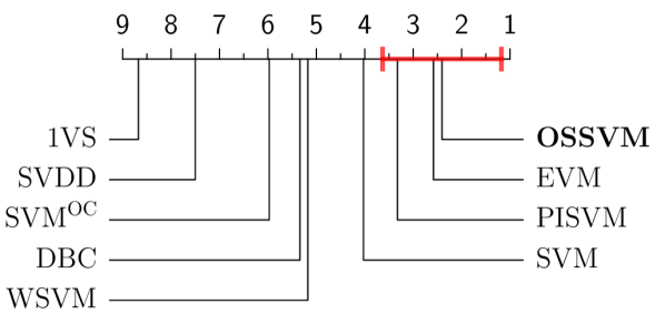
(a) Normalized accuracy.

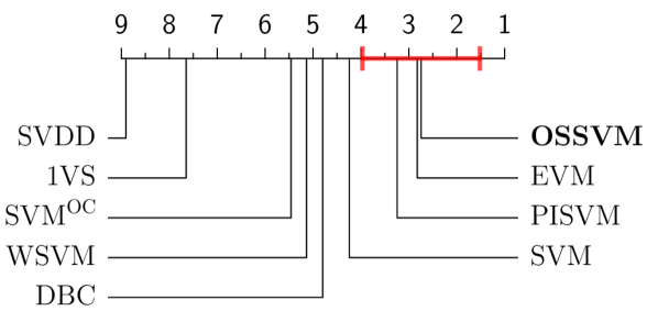
(b) Harmonic normalized accuracy.

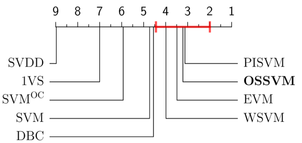
(c) Macro-averaging open-set f-measure.

(d) Micro-averaging open-set f-measure.

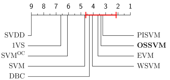
(e) Macro-averaging f-measure.

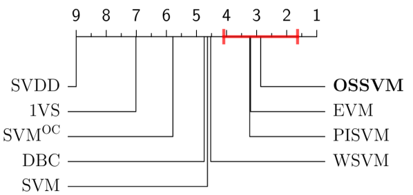
(f) Micro-averaging f-measure.

Figure 6: Critical difference diagram for comparison of OSSVM with baselines by employing Bonferroni-Dunn post-hoc test. The bold-red bar along the horizontal numeric axis in each figure covers the methods with no statistical difference from OSSVM

IV-F Remarks

It is remarkable the frequency of negative bias terms in the binary classifiers that compose the multiclass-from-binary one-vs-all SVM. Most of the binary classifiers for the one-vs-all approach already have the correct negative bias term, as shown in Table III. To better understand the reason, we also obtained the frequency of binary classifiers with negative bias term using the one-vs-one approach, also shown in Table III. In this case, only about half of the binary classifiers have negative bias term.

An informal explanation for this behavior is that in the one-vs-all approach, we have more negative than positive samples—and more than one class in the negative set. Then, it is more likely to have the negative samples “surround” the positive ones helping the SVM to create a bounded PLOS for the positive class. This intuition is confirmed by Figure 4. For both class 1 and class 2, the SVM creates a bounded PLOS (negative bias term) because class 3 (blue) is negative for those binary classifiers and it surrounds the positive class in both cases. Considering class 3 as positive, we have no negative samples surround the positive class. That is why, in this case, the PLOS is unbounded (non-negative bias term).

The high frequency of negative bias term for the one-vs-all explains why some authors in the literature have been reporting good accuracy for detection problems using SVM s with RBF kernels. For a detection problem, we have one class of interest and multiple others that we consider as negative for what we have access to train with. As the number of negative samples is usually larger, it is more likely to have a classifier with bounded PLOS for detection problems.

	SVM one-vs-all	SVM one-vs-one
yeast	93.33%	26.40%
mfeat-morphological	98.33%	39.66%
mfeat-zernike	98.33%	47.11%
mfeat-karhunen	98.89%	62.13%
mfeat-fourier	97.78%	57.70%
mfeat-factors	99.44%	41.82%
led7	100.0%	57.36%
led24	100.0%	50.00%
optdigits	99.44%	69.25%
pendigits	96.11%	64.25%
CIFAR10	100.0%	38.70%
MNIST	99.44%	43.52%
vowel	98.33%	67.10%
movement_libras	100.0%	49.96%
15-Scenes	99.00%	56.92%
KRKOPT	95.67%	40.25%
Letter	99.67%	55.75%
KDDCUP	99.33%	49.79%
Auslan	99.00%	42.50%
Caltech-256	98.00%	48.75%
ImageNet	99.33%	45.08%
ALOI	97.67%	52.50%
Mean	98.50%	50.30%

TABLE III: Percentage of binary classifiers with negative bias term per dataset for one-vs-all and one-vs-one approaches.

Despite most of the cases the SVM obtains the correct bias term for the one-vs-all approach, the optimization problem presented in Section III also optimizes the risk of the unknown. That is, it optimizes for recognition in open-set scenario.

V Conclusions and Future Work

In this work, we presented sufficient and necessary conditions for the SVM with RBF kernel to have a finite risk of the unknown. We then showed that by reformulating the RBF SVM optimization policy to simultaneously optimize margin and ensure a negative bias term, the risk of the unknown is bounded and it provides a formal open-set recognition algorithm.

The proposed OSSVM method extends upon the traditional SVM’s optimization problem. The objective function is changed in the primal problem, but the Lagrangian for the dual problem remains the same. In the dual problem for the OSSVM, only a single constraint differs from the SVM’s dual problem. Therefore, the same Sequential Minimal Optimization (SMO) algorithm [52] can be used to ensure the new constraint is satisfied between iterations. Also, the same Working Set Selection (WSS) algorithm [53] can be applied.

A limitation of the proposed method is that it can only be applied to specific kinds of kernel: the ones that tends to zero as the two given instances get far apart from each other. Among the well-known kernels, only RBF has this property, but others are available, e.g., Generalized T-Student, Rational Quadratic, and Inverse Multiquadric kernels [48]. Another limitation of this work is the lack of a proof that ensures the parameters selected during grid search phase can always generate a model, on the training phase, which has a negative bias term for bounding KLOS.

As future work, one can investigate alternative forms for ensuring a bounded PLOS for specific implementations of SVM s that do not rely on the bias term—as the ones in Vogt [49] and Kecman et al. [50]. As discussed in Section III-B, the SVM without the bias term cannot ensure a bounded PLOS, as it depends on the shape of the training data. However, a simple solution can be obtained by training the SVM without bias term and establishing an artificial negative bias term in the decision function. In this case, research can be done on how to obtain this artificial bias term. Another alternative is to consider an optimization problem with a fixed negative bias term [52].

Another future work is to investigate properties of the multiclass-from-binary SVM with the one-vs-one approach. In a binary SVM, at least one of the two classes will always have infinite PLOS—if one is bounded, the other must include all the remaining space and so it must be infinite. We observed experimentally that, according to the way the probability is calculated for each binary classifier [77, 78] and according to the way the probability estimates are combined in the multiclass-from-binary level [79], depending on the threshold established, a bounded KLOS can occur but cannot be ensured. Future work relies on investigating mechanisms to always ensure a bounded KLOS for one-vs-one approach and, consequently, a limited risk of the unknown. This is worth investigating because some works in the literature have presented better results with the one-vs-one than one-vs-all approach for closed-set problems [80]. We then hypothesize that, for one-vs-one approach, this investigation should be accomplished in the probability estimation or/and probability combination.

Finally, the guarantees we present in this work are valid for the feature space of the feature description. Ensuring a bounded mapping from the original feature space of the data to the space of feature description remains an open research problem associated to each description method.

Appendix A Complete OSSVM Formulation

The optimization problem for the OSSVM classifier is defined as

$$\min_{\mathbf{w},b,\xi}\ \frac{1}{2}\|\mathbf{w}\|^{2}+C\sum_{i=1}^{m}\xi_{i}+\lambda b,$$

s.t. $$y_{i}\left(\mathbf{w}^{T}\mathbf{x}_{i}+b\right)-1+\xi_{i}\geq 0,$$

$$\xi_{i}\geq 0.$$

Using the Lagrangian method, we have the Lagrangian defined as

$$\mathcal{L}(\mathbf{w},b,\xi,\alpha,\mathbf{r}) =\frac{1}{2}\|\mathbf{w}\|^{2}+C\sum_{i=1}^{m}\xi_{i}+\lambda b-\sum_{i=1}^{m}r_{i}\xi_{i}$$

$$-\sum_{i=1}^{m}\alpha_{i}\left[y_{i}\left(\mathbf{w}^{T}\mathbf{x}_{i}+b\right)-1+\xi_{i}\right],$$ (17)

in which $\alpha_{i}\in\mathbb{R}$ and $r_{i}\in\mathbb{R}$, $i=1,\dots,m$, are the Lagrangian multipliers.

First we want to minimize with respect to $\mathbf{w}$, $b$, and $\xi_{i}$, then we must ensure

$$\nabla_{\mathbf{w}}=\frac{\partial}{\partial b}\mathcal{L}=\frac{\partial}{\partial\xi_{i}}\mathcal{L}=0.$$

Consequently, we have

$$\mathbf{w}-\sum_{i=1}^{m}\alpha_{i}y_{i}\mathbf{x}_{i}=0\implies\mathbf{w}=\sum_{i=1}^{m}\alpha_{i}y_{i}\mathbf{x}_{i},$$ (18)

$$\lambda-\sum_{i=1}^{m}\alpha_{i}y_{i}=0\implies\sum_{i=1}^{m}\alpha_{i}y_{i}=\lambda,$$ (19)

$$C-\alpha_{i}-r_{i}=0\implies r_{i}=C-\alpha_{i}.$$ (20)

As the Lagrangian multipliers $\alpha_{i},r_{i}$ must be greater than 0, from Equation (20) we have the constraint $0\leq\alpha_{i}\leq C$ as a consequence of the soft margin formulation in the dual problem. This is the same constraint we have in the traditional formulation of the SVM classifier.

Using Equations (18)–(20) to simplify the Lagrangian in Equation (A), we have

$$\mathcal{L}(\mathbf{w},b,\xi,\alpha) =\frac{1}{2}\sum_{i=1}^{m}\sum_{j=1}^{m}\alpha_{i}\alpha_{i}y_{i}y_{j}\mathbf{x}_{i}^{T}\mathbf{x}_{j}+C\sum_{i=1}^{m}\xi_{i}$$

$$+b\sum_{i=1}^{m}\alpha_{i}y_{i}-C\sum_{i=1}^{m}\xi_{i}+\sum_{i=1}^{m}\alpha_{i}\xi_{i}$$

$$-\sum_{i=1}^{m}\sum_{j=1}^{m}\alpha_{i}\alpha_{i}y_{i}y_{j}\mathbf{x}_{i}^{T}\mathbf{x}_{j}-b\sum_{i=1}^{m}\alpha_{i}y_{i}$$

$$+\sum_{i=1}^{m}\alpha_{i}-\sum_{i=1}^{m}\alpha_{i}\xi_{i},$$

which simplifies to

$$\mathcal{L}(\alpha) =\sum_{i=1}^{m}\alpha_{i}-\frac{1}{2}\sum_{i=1}^{m}\sum_{j=1}^{m}\alpha_{i}\alpha_{i}y_{i}y_{j}\mathbf{x}_{i}^{T}\mathbf{x}_{j}$$

$$=\sum_{i=1}^{m}\alpha_{i}-\frac{1}{2}\|\mathbf{w}\|^{2}.$$ (21)

Equation (21) shows the same Lagrangian of the traditional SVM optimization problem. The optimization of the bias term $b$ relies on the constraint in Equation (19).

Therefore, the dual optimization problem is defined as

$$\min_{\alpha}\ \mathcal{W}(\alpha)=-\mathcal{L}(\alpha)=\frac{1}{2}\|\mathbf{w}\|^{2}-\sum_{i=1}^{m}\alpha_{i},$$

s.t. $$0<\alpha_{i}<C,\ \forall i,$$

$$\sum_{i=1}^{m}\alpha_{i}y_{i}=\lambda.$$

Pedro Ribeiro Mendes Júnior is a postdoctoral researcher at Institute of Computing at the University of Campinas. He received his PhD (2018) and MSc (2014) in Computer Science by the same university. He has passed part of his PhD in an internship at University of Colorado, Colorado Springs, with the supervision of Prof. Terrance Boult, period in which the OSSVM method was most formalized. He stayed for a short post-doctoral internship at Politecnico di Milano working with Prof. Stefano Tubaro and Prof. Paolo Bestagini, period in which OSSVM was applied with success for other applications. He obtained his Bachelor’s in Computer Science at the Federal University of Ouro Preto (Universidade Federal de Ouro Preto), period in which he has worked mainly on image processing and computer vision. His current research topics are open-set recognition, computer vision, neural networks, time-series forecasting, time-series anomaly detection, etc. and on living consciously.

Terrance E. Boult is a Distinguished Professor and the El Pomar Endowed Professor of Innovation and Security at U. Colorado Colorado Springs, as well as being an IEEE fellow and a serial entrepreneur and internationally acknowledged researcher in machine learning, computer vision, biometrics, and cybersecurity with 15 patents issued, 400+ papers. He received his BS in Applied Math (1983), MS in CS (1984), and Ph.D. in Computer CS (1986) from Columbia University and then spent six years as an Assistant Prof and two years as an Assoc. Prof in Columbia’s CS Department. He moved from Columbia to Lehigh (1994-2003), where he was an endowed professor and eventually founded Lehigh’s CS department. He joined UCCS in 2003 as an El Pomar Professor. Over his career, he has won multiple teaching awards, research/innovation awards, best paper awards, best reviewer awards, and IEEE service awards; He is a member of the IEEE Golden Core and has been an IEEE Distinguished Lecturer, and in 2017 was elected as an IEEE Fellow. He was a co-founder of the Computer Vision Foundation and very active in organizing/managing Computer Vision conferences. On the education side, Dr. Boult is the founder, primary architect, and co-director of the world’s first and only Bachelor of Innovation™ Family of Degrees at UCCS. This awarding family of degrees combines a core of innovation and entrepreneurship with a significant multi-year ”team emphasis” and all the rigor of bachelor degrees in their fields, serving 100s or students across 22 different majors spanning four colleges.

Jacques Wainer is a professor at the Computing Institute at the State University of Campinas. He received his PH.D in Computer Science in 1991 from the Pennsylvania State University. He has worked in areas such as collaborative computing, medical informatics, bibliometrics, social impacts of computers, and others. Currently, his main focus of research is machine learning.

Anderson Rocha is an Associate Professor at the Institute of Computing, University of Campinas (Unicamp), Brazil, since 2009. He obtained his bachelor’s degree (2003) in Computer Science at Federal University of Lavras, Brazil. He obtained his M.Sc. (2006) and Ph.D. (2009) in Computer Science at Unicamp. His research interests include Machine Learning, Reasoning for Complex Data, and Digital Forensics. He is an IEEE Senior member and the Chair of the IEEE Information Forensics and Security Technical Committee (IFS-TC) for the 2019-2020 term. He has been actively involved in the organization of several events such as ICIP, ICASSP, WIFS in the past years and has been an Associate Editor of several journals such as the IEEE Security & Privacy, IEEE Signal Processing Letters, and the IEEE Transactions on Information Forensics and Security, and a Senior Editor for the IEEE Signal Processing Letters. He is a Microsoft, Google, and Tan Chi Tuan Faculty Fellow, honorable recognitions for his research contributions.

References

- Bishop [2006] C. M. Bishop, Pattern Recognition and Machine Learning, 1st ed., ser. Information Science and Statistics. Springer-Verlag New York, 2006.
- Breiman [2001] L. Breiman, “Random Forests,” Springer Machine Learning, vol. 45, no. 1, pp. 5–32, Oct. 2001.
- Cortes and Vapnik [1995] C. Cortes and V. Vapnik, “Support-vector networks,” Springer Machine Learning, vol. 20, no. 3, pp. 273–297, Sep. 1995.
- LeCun et al. [2015] Y. LeCun, Y. Bengio, and G. Hinton, “Deep learning,” Nature, vol. 521, no. 7553, pp. 436–444, May 2015.
- Costa et al. [2014] F. d. O. Costa, E. Silva, M. Eckmann, W. J. Scheirer, and A. Rocha, “Open set source camera attribution and device linking,” Elsevier Pattern Recognition Letters, vol. 39, pp. 92–101, Apr. 2014.
- Ferreira et al. [2017] A. Ferreira, L. Bondi, L. Baroffio, P. Bestagini, J. Huang, J. A. dos Santos, S. Tubaro, and A. Rocha, “Data-driven feature characterization techniques for laser printer attribution,” IEEE Transactions on Information Forensics and Security, vol. 12, no. 8, pp. 1860–1873, Aug. 2017.
- Dubuisson and Masson [1993] B. Dubuisson and M. Masson, “A statistical decision rule with incomplete knowledge about classes,” Elsevier Pattern Recognition, vol. 26, no. 1, pp. 155–165, Jan. 1993.
- Muzzolini et al. [1998] R. Muzzolini, Y.-H. Yang, and R. Pierson, “Classifier design with incomplete knowledge,” Elsevier Pattern Recognition, vol. 31, no. 4, pp. 345–369, Apr. 1998.
- Moeini et al. [2017] A. Moeini, K. Faez, H. Moeini, and A. M. Safai, “Open-set face recognition across look-alike faces in real-world scenarios,” Elsevier Image and Vision Computing, vol. 57, pp. 1–14, Jan. 2017.
- Mendes Júnior et al. [2017] P. R. Mendes Júnior, R. M. de Souza, R. d. O. Werneck, B. V. Stein, D. V. Pazinato, W. R. de Almeida, O. A. B. Penatti, R. d. S. Torres, and A. d. R. Rocha, “Nearest neighbors distance ratio open-set classifier,” Springer Machine Learning, vol. 106, no. 3, pp. 359–386, Mar. 2017.
- Liu et al. [2017] W. Liu, Y. Wen, Z. Yu, M. Li, B. Raj, and L. Song, “SphereFace: Deep hypersphere embedding for face recognition,” in IEEE International Conference on Computer Vision and Pattern Recognition, Honolulu, HI, USA, Jul. 2017, pp. 212–220.
- Wen et al. [2019] Y. Wen, K. Zhang, Z. Li, and Y. Qiao, “A comprehensive study on center loss for deep face recognition,” Springer International Journal of Computer Vision, vol. 127, no. 6–7, pp. 668–683, Jun. 2019.
- Tax and Duin [2004] D. M. J. Tax and R. P. W. Duin, “Support vector data description,” Springer Machine Learning, vol. 54, no. 1, pp. 45–66, Jan. 2004.
- Chang et al. [2013] W.-C. Chang, C.-P. Lee, and C.-J. Lin, “A revisit to Support Vector Data Description,” National Taiwan University of Science and Technology, Taipei, Taiwan, Tech. Rep., 2013.
- Schölkopf et al. [2001] B. Schölkopf, J. C. Platt, J. Shawe-Taylor, A. J. Smola, and R. C. Williamson, “Estimating the support of a high-dimensional distribution,” Neural Computation, vol. 13, no. 7, pp. 1443–1471, Jul. 2001.
- Cortes et al. [2016] C. Cortes, G. DeSalvo, and M. Mohri, “Learning with rejection,” in International Conference on Algorithmic Learning Theory, ser. Lecture Notes in Computer Science, R. Ortner, H. U. Simon, and S. Zilles, Eds., vol. 9925. Bari, Italy: Springer International Publishing, Oct. 2016, pp. 67–82.
- Rocha and Goldenstein [2014] A. Rocha and S. Goldenstein, “Multiclass from binary: Expanding one-vs-all, one-vs-one and ECOC-based approaches,” IEEE Transactions on Neural Networks and Learning Systems, vol. 25, no. 2, pp. 289–302, Feb. 2014.
- Pritsos and Stamatatos [2013] D. A. Pritsos and E. Stamatatos, “Open-set classification for automated genre identification,” in European Conference on Information Retrieval, ser. Lecture Notes in Computer Science, P. Serdyukov, P. Braslavski, S. O. Kuznetsov, J. Kamps, and S. Rüger, Eds., vol. 7814. Moscow, Russia: Springer, Berlin, Heidelberg, Mar. 2013, pp. 207–217.
- Scheirer et al. [2014] W. J. Scheirer, L. P. Jain, and T. E. Boult, “Probability models for open set recognition,” IEEE Transactions on Pattern Analysis and Machine Intelligence, vol. 36, no. 11, pp. 2317–2324, Nov. 2014.
- Jain et al. [2014] L. P. Jain, W. J. Scheirer, and T. E. Boult, “Multi-class open set recognition using probability of inclusion,” in European Conference on Computer Vision, ser. Lecture Notes in Computer Science, D. Fleet, T. Pajdla, B. Schiele, and T. Tuytelaars, Eds., vol. 8691, part III. Zurich, Switzerland: Springer, Cham, Sep. 2014, pp. 393–409.
- Scheirer et al. [2013] W. J. Scheirer, A. d. R. Rocha, A. Sapkota, and T. E. Boult, “Towards open set recognition,” IEEE Transactions on Pattern Analysis and Machine Intelligence, vol. 35, no. 7, pp. 1757–1772, Jul. 2013.
- Heflin et al. [2012] B. Heflin, W. J. Scheirer, and T. E. Boult, “Detecting and classifying scars, marks, and tattoos found in the wild,” in IEEE International Conference on Biometrics: Theory, Applications and Systems, Arlington, VA, USA, Sep. 2012, pp. 31–38.
- Mendes Júnior et al. [2019] P. R. Mendes Júnior, L. Bondi, P. Bestagini, S. Tubaro, and A. Rocha, “An in-depth study on open-set camera model identification,” IEEE Access, vol. 7, pp. 180 713–180 726, Jun. 2019.
- Costa et al. [2012] F. d. O. Costa, M. Eckmann, W. J. Scheirer, and A. Rocha, “Open set source camera attribution,” in Conference on Graphics, Patterns, and Images. Ouro Preto, MG, Brazil: IEEE Press, Aug. 2012, pp. 71–78.
- Coles [2001] S. Coles, An Introduction to Statistical Modeling of Extreme Values, 1st ed., ser. Springer Series in Statistics. Springer, London, 2001.
- Rudd et al. [2018] E. M. Rudd, L. P. Jain, W. J. Scheirer, and T. E. Boult, “The Extreme Value Machine,” IEEE Transactions on Pattern Analysis and Machine Intelligence, vol. 40, no. 3, pp. 762–768, Mar. 2018.
- Scheirer [2017] W. J. Scheirer, Extreme Value Theory-Based Methods for Visual Recognition, 1st ed., ser. Synthesis Lectures on Computer Vision. Morgan & Claypool Publishers, Feb. 2017.
- Vareto et al. [2017] R. Vareto, S. Silva, F. Costa, and W. R. Schwartz, “Towards open-set face recognition using hashing functions,” in IEEE International Joint Conference on Biometrics, Denver, CO, USA, Oct. 2017, pp. 634–641.
- Busto and Gall [2017] P. P. Busto and J. Gall, “Open set domain adaptation,” in IEEE International Conference on Computer Vision, Venice, Italy, Oct. 2017, pp. 754–763.
- Saito et al. [2018] K. Saito, S. Yamamoto, Y. Ushiku, and T. Harada, “Open set domain adaptation by backpropagation,” in European Conference on Computer Vision, ser. Lecture Notes in Computer Science, V. Ferrari, M. Hebert, C. Sminchisescu, and Y. Weiss, Eds., vol. 11205. Munich, Germany: Springer, Cham, Sep. 2018, pp. 156–171.
- Fu et al. [2019] J. Fu, X. Wu, S. Zhang, and J. Yan, “Improved open set domain adaptation with backpropagation,” in IEEE International Conference on Image Processing, Taipei, Taiwan, Sep. 2019, pp. 2506–2510.
- Liu et al. [2019] H. Liu, Z. Cao, M. Long, J. Wang, and Q. Yang, “Separate to adapt: Open set domain adaptation via progressive separation,” in IEEE International Conference on Computer Vision and Pattern Recognition. Long Beach, CA, USA: IEEE, Jun. 2019, pp. 2922–2931.
- Neira et al. [2018] M. A. C. Neira, P. R. Mendes Júnior, A. Rocha, and R. d. S. Torres, “Data-fusion techniques for open-set recognition problems,” IEEE Access, vol. 6, pp. 21 242–21 265, Apr. 2018.
- Dhamija et al. [2020] A. Dhamija, M. Günther, J. Ventura, and T. Boult, “The overlooked elephant of object detection: Open set,” in Winter Conference on Applications of Computer Vision. Aspen, CO, USA: IEEE Press, Mar. 2020, pp. 1021–1030.
- Dang et al. [2019] S. Dang, Z. Cao, Z. Cui, Y. Pi, and N. Liu, “Open set incremental learning for automatic target recognition,” IEEE Transactions on Geoscience and Remote Sensing, vol. 57, no. 7, pp. 4445–4456, Jul. 2019.
- Moraes et al. [2016] D. Moraes, J. Wainer, and A. Rocha, “Low false positive learning with Support Vector Machines,” Elsevier Journal of Visual Communication and Image Representation, vol. 38, pp. 340–350, Jul. 2016.
- Tax and Duin [2008] D. M. J. Tax and R. P. W. Duin, “Growing a multi-class classifier with a reject option,” Elsevier Pattern Recognition Letters, vol. 29, no. 10, pp. 1565–1570, Jul. 2008.
- Bartlett and Wegkamp [2008] P. L. Bartlett and M. H. Wegkamp, “Classification with a reject option using a hinge loss,” Journal of Machine Learning Research, vol. 9, pp. 1823–1840, Aug. 2008.
- Saki et al. [2019] F. Saki, Y. Guo, C.-Y. Hung, L.-h. Kim, M. Deshpande, S. Moon, E. Koh, and E. Visser, “Open-set evolving acoustic scene classification system,” in Detection and Classification of Acoustic Scenes and Events Workshop, New York, NY, USA, Oct. 2019, pp. 219–223.
- Tornai and Scheirer [2019] K. Tornai and W. J. Scheirer, “Gesture-based user identity verification as an open set problem for smartphones,” in IAPR International Conference on Biometrics, Crete, Greece, Jun. 2019, pp. 1–8.
- Yang et al. [2019] Y. Yang, C. Hou, Y. Lang, D. Guan, D. Huang, and J. Xu, “Open-set human activity recognition based on micro-Doppler signatures,” Elsevier Pattern Recognition, vol. 85, pp. 60–69, Jan. 2019.
- Geng et al. [2020] C. Geng, S.-J. Huang, and S. Chen, “Recent advances in open set recognition: A survey,” IEEE Transactions on Pattern Analysis and Machine Intelligence, pp. 1–19, Mar. 2020, early Access.
- Boser et al. [1992] B. E. Boser, I. M. Guyon, and V. N. Vapnik, “A training algorithm for optimal margin classifiers,” in ACM Annual Workshop on Computational Learning Theory, Pittsburgh, PA, USA, Jul. 1992, pp. 144–152.
- Mercer [1909] J. Mercer, “Functions of positive and negative type, and their connection the theory of integral equations,” Philosophical Transactions of the Royal Society A, vol. 209, no. 441–458, pp. 415–446, Jan. 1909.
- Schölkopf and Smola [2001] B. Schölkopf and A. J. Smola, Learning with Kernels, 1st ed., ser. Adaptive Computation and Machine Learning series. MIT Press, Dec. 2001.
- Chang and Lin [2011] C.-C. Chang and C.-J. Lin, “LIBSVM: A library for Support Vector Machines,” ACM Transactions on Intelligent Systems and Technology, vol. 2, no. 3, pp. 27:1–27:27, Apr. 2011.
- Buhmann [2003] M. D. Buhmann, Radial Basis Functions: Theory and Implementations, 1st ed., ser. Cambridge Monographs on Applied and Computational Mathematics. Cambridge University Press, Jul. 2003.
- Souza [2010] C. R. Souza, “Kernel functions for machine learning applications,” Mar. 2010, accessed: November 14, 2018. [Online]. Available: http://crsouza.com/2010/03/17/kernel-functions-for-machine-learning-applications
- Vogt [2002] M. Vogt, “SMO algorithms for Support Vector Machines without bias term,” Institute of Automatic Control, Technische Universität Darmstadt, Darmstadt, Germany, Tech. Rep., Jul. 2002.
- Kecman et al. [2005] V. Kecman, T. M. Huang, and M. Vogt, “Iterative single data algorithm for training kernel machines from huge data sets: Theory and performance,” in Support Vector Machines: Theory and Applications, ser. Studies in Fuzziness and Soft Computing, L. Wang, Ed. Springer, Berlin, Heidelberg, Apr. 2005, vol. 177, pp. 255–274.
- Kuncheva and Hadjitodorov [2004] L. I. Kuncheva and S. T. Hadjitodorov, “Using diversity in cluster ensembles,” in IEEE International Conference on Systems, Man, and Cybernetics, vol. 2, The Hague, Netherlands, Oct. 2004, pp. 1214–1219.
- Platt [1998] J. C. Platt, “Fast training of Support Vector Machines using Sequential Minimal Optimization,” in Advances in Kernel Methods: Support Vector Learning, 1st ed., B. Schölkopf, C. J. C. Burges, and A. J. Smola, Eds. MIT Press, Dec. 1998, ch. 12, pp. 185–208.
- Fan et al. [2005] R.-E. Fan, P.-H. Chen, and C.-J. Lin, “Working Set Selection using second order information for training Support Vector Machines,” Journal of Machine Learning Research, vol. 6, pp. 1889–1918, Dec. 2005.
- Sokolova and Lapalme [2009] M. Sokolova and G. Lapalme, “A systematic analysis of performance measures for classification tasks,” Elsevier Information Processing & Management, vol. 45, no. 4, pp. 427–437, Jul. 2009.
- Mitchell [2004] D. W. Mitchell, “More on spreads and non-arithmetic means,” The Mathematical Gazette, vol. 88, no. 511, pp. 142–144, Mar. 2004.
- Lazebnik et al. [2006] S. Lazebnik, C. Schmid, and J. Ponce, “Beyond bags of features: Spatial pyramid matching for recognizing natural scene categories,” in IEEE International Conference on Computer Vision and Pattern Recognition, vol. 2, New York, NY, USA, Jun. 2006, pp. 2169–2178.
- van Gemert et al. [2010] J. C. van Gemert, C. J. Veenman, A. W. M. Smeulders, and J.-M. Geusebroek, “Visual word ambiguity,” IEEE Transactions on Pattern Analysis and Machine Intelligence, vol. 32, no. 7, pp. 1271–1283, Jul. 2010.
- Boureau et al. [2010] Y.-L. Boureau, F. Bach, Y. LeCun, and J. Ponce, “Learning mid-level features for recognition,” in IEEE International Conference on Computer Vision and Pattern Recognition, San Francisco, CA, USA, Jun. 2010, pp. 2559–2566.
- Lowe [2004] D. Lowe, “Distinctive image features from scale-invariant keypoints,” Springer International Journal of Computer Vision, vol. 60, no. 2, pp. 91–110, Nov. 2004.
- Frey and Slate [1991] P. W. Frey and D. J. Slate, “Letter recognition using Holland-style adaptive classifiers,” Springer Machine Learning, vol. 6, no. 2, pp. 161–182, Mar. 1991.
- Michie et al. [1994] D. Michie, D. J. Spiegelhalter, and C. C. Taylor, Machine Learning, Neural and Statistical Classification, ser. Ellis Horwood Series in Artificial Intelligence. Upper Saddle River, NJ, USA: Prentice Hall, Jul. 1994.
- Stolfo et al. [2000] S. J. Stolfo, W. Fan, W. Lee, A. Prodromidis, and P. K. Chan, “Cost-based modeling for fraud and intrusion detection: Results from the JAM project,” in DARPA Information Survivability Conference and Exposition, vol. 2. Hilton Head, SC, USA: IEEE Press, Jan. 2000, pp. 130–144.
- Kadous [2002] M. W. Kadous, “Temporal classification: Extending the classification paradigm to multivariate time series,” Ph.D. dissertation, The University of New South Wales, New South Wales, Australia, Oct. 2002.
- Griffin et al. [2007] G. Griffin, A. Holub, and P. Perona, “Caltech-256 object category dataset,” California Institute of Technology, Tech. Rep., May 2007.
- Geusebroek et al. [2005] J.-M. Geusebroek, G. J. Burghouts, and A. W. M. Smeulders, “The Amsterdam library of object images,” Springer International Journal of Computer Vision, vol. 61, no. 1, pp. 103–112, Jan. 2005.
- Stehling et al. [2002] R. O. Stehling, M. A. Nascimento, and A. X. Falcão, “A compact and efficient image retrieval approach based on border/interior pixel classification,” in ACM International Conference on Information and Knowledge Management, McLean, VA, USA, Nov. 2002, pp. 102–109.
- Russakovsky et al. [2015] O. Russakovsky, J. Deng, H. Su, J. Krause, S. Satheesh, S. Ma, Z. Huang, A. Karpathy, A. Khosla, M. Bernstein, A. C. Berg, and L. Fei-Fei, “ImageNet large scale visual recognition challenge,” Springer International Journal of Computer Vision, vol. 115, no. 3, pp. 211–252, Dec. 2015.
- Bendale and Boult [2016] A. Bendale and T. E. Boult, “Towards open set deep networks,” in IEEE International Conference on Computer Vision and Pattern Recognition, Las Vegas, NV, USA, Jun. 2016, pp. 1563–1572.
- Szegedy et al. [2015] C. Szegedy, W. Liu, Y. Jia, P. Sermanet, S. Reed, D. Anguelov, D. Erhan, V. Vanhoucke, and A. Rabinovich, “Going deeper with convolutions,” in IEEE International Conference on Computer Vision and Pattern Recognition, Boston, MA, USA, Jun. 2015, pp. 1–9.
- Tipping and Bishop [1999] M. E. Tipping and C. M. Bishop, “Probabilistic principal component analysis,” Journal of the Royal Statistical Society: Series B (Statistical Methodology), vol. 61, no. 3, pp. 611–622, 1999.
- Krizhevsky and Hinton [2009] A. Krizhevsky and G. Hinton, “Learning multiple layers of features from tiny images,” Master’s thesis, University of Toronto, Apr. 2009.
- LeCun et al. [1998] Y. LeCun, L. Bottou, Y. Bengio, and P. Haffner, “Gradient-based learning applied to document recognition,” Proceedings of the IEEE, vol. 86, no. 11, pp. 2278–2324, Nov. 1998.
- Tensorflow.org [2018a] Tensorflow.org, “Advanced Convolutional Neural Networks,” Oct. 2018, accessed: November 14, 2018. [Online]. Available: https://www.tensorflow.org/tutorials/images/deep_cnn
- Tensorflow.org [2018b] ——, “Deep MNIST for experts,” May 2018, backup version. Accessed: November 14, 2018. [Online]. Available: https://apimirror.com/tensorflow~guide/get_started/mnist/pros
- Olson et al. [2017] R. S. Olson, W. La Cava, P. Orzechowski, R. J. Urbanowicz, and J. H. Moore, “PMLB: A large benchmark suite for machine learning evaluation and comparison,” BioData Mining, vol. 10, no. 36, pp. 1–13, Dec. 2017.
- Demšar [2006] J. Demšar, “Statistical comparisons of classifiers over multiple data sets,” Journal of Machine Learning Research, vol. 7, pp. 1–30, Jan. 2006.
- Platt [2000] J. C. Platt, “Probabilities for SV Machines,” in Advances in Large-Margin Classifiers, ser. Neural Information Processing series, A. J. Smola, P. Bartlett, B. Schölkopf, and D. Schuurmans, Eds. MIT Press, Sep. 2000, ch. 5, pp. 61–74.
- Lin et al. [2007] H.-T. Lin, C.-J. Lin, and R. C. Weng, “A note on Platt’s probabilistic outputs for Support Vector Machines,” Springer Machine Learning, vol. 68, no. 3, pp. 267–276, Oct. 2007.
- Wu et al. [2004] T.-F. Wu, C.-J. Lin, and R. C. Weng, “Probability estimates for multi-class classification by pairwise coupling,” Journal of Machine Learning Research, vol. 5, pp. 975–1005, Aug. 2004.
- Galar et al. [2011] M. Galar, A. Fernández, E. Barrenechea, H. Bustince, and F. Herrera, “An overview of ensemble methods for binary classifiers in multi-class problems: Experimental study on one-vs-one and one-vs-all schemes,” Elsevier Pattern Recognition, vol. 44, no. 8, pp. 1761–1776, Aug. 2011.
- Hunter [2007] J. D. Hunter, “Matplotlib: A 2D graphics environment,” Computing in Science & Engineering, vol. 9, no. 3, pp. 90–95, Jun. 2007.
- Perez and Granger [2007] F. Perez and B. E. Granger, “IPython: A system for interactive scientific computing,” Computing in Science & Engineering, vol. 9, no. 3, pp. 21–29, Jun. 2007.
- Pedregosa et al. [2011] F. Pedregosa, G. Varoquaux, A. Gramfort, V. Michel, B. Thirion, O. Grisel, M. Blondel, P. Prettenhofer, R. Weiss, V. Dubourg, J. Vanderplas, A. Passos, D. Cournapeau, M. Brucher, M. Perrot, and É. Duchesnay, “Scikit-learn: Machine learning in Python,” Journal of Machine Learning Research, vol. 12, pp. 2825–2830, Oct. 2011.
- Albanese et al. [2012] D. Albanese, R. Visintainer, S. Merler, S. Riccadonna, G. Jurman, and C. Furlanello, “mlpy: Machine Learning Python,” CoRR, vol. abs/1202.6548, pp. 1–4, Mar. 2012.
- Demšar et al. [2013] J. Demšar, T. Curk, A. Erjavec, Č. Gorup, T. Hočevar, M. Milutinovič, M. Možina, M. Polajnar, M. Toplak, A. Starič, M. Štajdohar, L. Umek, L. Žagar, J. Žbontar, M. Žitnik, and B. Zupan, “Orange: Data mining toolbox in Python,” Journal of Machine Learning Research, vol. 14, pp. 2349–2353, Aug. 2013.
- Tange [2018] O. Tange, “GNU parallel 2018,” GNU’s Not Unix, Tech. Rep., Apr. 2018.